The continuous categorical: a novel simplex-valued exponential family
Abstract
Simplex-valued data appear throughout statistics and machine learning, for example in the context of transfer learning and compression of deep networks. Existing models for this class of data rely on the Dirichlet distribution or other related loss functions; here we show these standard choices suffer systematically from a number of limitations, including bias and numerical issues that frustrate the use of flexible network models upstream of these distributions. We resolve these limitations by introducing a novel exponential family of distributions for modeling simplex-valued data – the continuous categorical, which arises as a nontrivial multivariate generalization of the recently discovered continuous Bernoulli. Unlike the Dirichlet and other typical choices, the continuous categorical results in a well-behaved probabilistic loss function that produces unbiased estimators, while preserving the mathematical simplicity of the Dirichlet. As well as exploring its theoretical properties, we introduce sampling methods for this distribution that are amenable to the reparameterization trick, and evaluate their performance. Lastly, we demonstrate that the continuous categorical outperforms standard choices empirically, across a simulation study, an applied example on multi-party elections, and a neural network compression task.111Our code is available at https://github.com/cunningham-lab/cb_and_cc
1 Introduction
Simplex-valued data, commonly referred to as compositional data in the statistics literature, are of great practical relevance across the natural and social sciences (see Pawlowsky-Glahn & Egozcue (2006); Pawlowsky-Glahn & Buccianti (2011); Pawlowsky-Glahn et al. (2015) for an overview). Prominent examples appear in highly cited work ranging from geology (Pawlowsky-Glahn & Olea, 2004; Buccianti et al., 2006), chemistry (Buccianti & Pawlowsky-Glahn, 2005), microbiology (Gloor et al., 2017), genetics (Quinn et al., 2018), psychiatry (Gueorguieva et al., 2008), ecology (Douma & Weedon, 2019), environmental science (Filzmoser et al., 2009), materials science (Na et al., 2014), political science (Katz & King, 1999), public policy (Breunig & Busemeyer, 2012), economics (Fry et al., 2000), and the list goes on. An application of particular interest in machine learning arises in the context of model compression, where the class probabilities outputted by a large model are used as ‘soft targets’ to train a small neural network (Buciluǎ et al., 2006; Ba & Caruana, 2014; Hinton et al., 2015), an idea used also in transfer learning (Tzeng et al., 2015; Parisotto et al., 2015).
The existing statistical models of compositional data come in three flavors. Firstly, there are models based on a Dirichlet likelihood, for example the Dirichlet GLM (Campbell & Mosimann, 1987; Gueorguieva et al., 2008; Hijazi & Jernigan, 2009) and Dirichlet Component Analysis (Wang et al., 2008; Masoudimansour & Bouguila, 2017). Secondly, there are also models based on applying classical statistical techniques to -valued transformations of simplex-valued data, notably via Logratios (Aitchison, 1982, 1994, 1999; Egozcue et al., 2003; Ma et al., 2016; Avalos et al., 2018). Thirdly, the machine learning literature has proposed predictive models that forgo the use of a probabilistic objective altogether and optimize the categorical cross-entropy instead (Ba & Caruana, 2014; Hinton et al., 2015; Sadowski & Baldi, 2018). The first type of model, fundamentally, suffers from an ill-behaved loss function (amongst other drawbacks) (§2), which constrain the practitioner to using inflexible (linear) models with only a small number of predictors. The second approach typically results in complicated likelihoods, which are hard to analyze and do not form an exponential family, forgoing many of the attractive theoretical properties of the Dirichlet. The third approach suffers from ignoring normalizing constants, sacrificing the properties of maximum likelihood estimation (see Loaiza-Ganem & Cunningham (2019) for a more detailed discussion of the pitfalls).
In this work, we resolve these limitations simultaneously by defining a novel exponential family supported on the simplex, the continuous categorical (CC) distribution. Our distribution arises naturally as a multivariate generalization of the recently discovered continuous Bernoulli (CB) distribution (Loaiza-Ganem & Cunningham, 2019), a -supported exponential family motivated by Variational Autoencoders (Kingma & Welling, 2014), which showed empirical improvements over the beta distribution for modeling data which lies close to the extrema of the unit interval.
Similarly, the CC will provide three crucial advantages over the Dirichlet and other competitors: it defines a coherent, well-behaved and computationally tractable log-likelihood (§3.1, 3.4), which does not blow up in the presence of zero-valued observations (§3.2), and which produces unbiased estimators (§3.3). Moreover, the CC model presents no added complexity relative to its competitors; it has one fewer parameter than the Dirichlet and a normalizing constant that can be written in closed form using elementary functions alone (§3.4). The continuous categorical brings probabilistic machine learning to the analysis of compositional data, opening up avenues for future applied and theoretical research.
2 Background
Careful consideration of the Dirichlet clarifies its shortcomings and the need for the CC family. The Dirichlet distribution is parameterized by and defined on the simplex by:
| (1) |
where denotes the multivariate beta function, and .222Note that the th component does not form part of the argument; it is a deterministic function of the -dimensional random variable .
This density function presents an attractive combination of mathematical simplicity, computational tractability, and the flexibility to model both interior modes and sparsity, as well as defining an exponential family of distributions that provides a multivariate generalization of the beta distribution and a conjugate prior to the multinomial distribution. As such, the Dirichlet is by far the best known and most widely used probability distribution for modeling simplex-valued random variables (Ng et al., 2011). This includes both the latent variables of mixed membership models (Erosheva, 2002; Blei et al., 2003; Barnard et al., 2003), and the statistical modeling of compositional outcomes (Aitchison, 1982; Campbell & Mosimann, 1987; Hijazi, 2003; Wang et al., 2008). Our work focuses on the latter, with special attention to the setting where we aim to learn a (possibly nonlinear) regression function that models a simplex-valued response in terms of a (possibly large) set of predictors. In this context, and in spite of its strengths, the Dirichlet distribution suffers from three fundamental limitations.
First, flexibility: while the ability to capture interior modes might seem intuitively appealing, in practice it thwarts the optimization of predictive models of compositional data (as we will demonstrate empirically in section §5.2). To illustrate why, consider fitting a Dirichlet distribution to a single observation lying inside the simplex. Maximizing the likelihood will lead to a point mass on the observed datapoint (as was also noted by Sadowski & Baldi (2018)); the log-likelihood will diverge, and so will the parameter estimate (tending to along the line that preserves the observed proportions). This example may seem degenerate; after all, any dataset that would warrant a probabilistic model had better contain more than a single observation, at which point no individual point can ‘pull’ the density onto itself. However, in the context of predictive modeling, observations will often present unique input-output pairs, particularly if we have continuous predictors, or a large number of categorical ones. Thus, any regression function that is sufficiently flexible, such as a deep network, or that takes a sufficiently large number of inputs, can result in a divergent log-likelihood, frustrating an optimizer’s effort to find a sensible estimator. This limitation has constrained Dirichlet-based predictive models to the space of linear functions (Campbell & Mosimann, 1987; Hijazi & Jernigan, 2009).
Second, tails: the Dirichlet density diverges or vanishes at the extrema for all but a set of measure zero values of , so that the log-likelihood is undefined whenever an observation contains zeros (transformation-based alternatives, such as Logratios, suffer the same drawback). However, zeros are ubiquitous in real-world compositional data, a fact that has lead to the development of numerous hacks, such as Palarea-Albaladejo & Martín-Fernández (2008); Scealy & Welsh (2011); Stewart & Field (2011); Hijazi et al. (2011); Tsagris & Stewart (2018), each of which carries its own tradeoffs.
Third, bias: an elementary result is that the MLE of an exponential family yields an unbiased estimator for its sufficient statistic. However, the sufficient statistic of the Dirichlet distribution is the logarithm of the data, so that by Jensen’s inequality, the MLE for the mean parameter, which is often the object of interest, is biased. While the MLE is also asymptotically consistent, this is only the case in the unrealistic setting of a true Dirichlet data-generating process, as we will illustrate empirically in section §5.1.
3 The continuous categorical distribution
These three limitations motivate the introduction of a novel exponential family, the continuous categorical (CC), which is defined on the closed simplex, , by:
| (2) |
where, again, . Without loss of generality we restrict the parameter values ; such a choice makes the model identifiable. The CC density looks much like the Dirichlet, except that we have switched the role of the parameter and the variable. However, this simple exchange results in a well-behaved log-likelihood that can no longer concentrate mass on single interior points (§3.1), nor diverge at the extrema (§3.2), and that produces unbiased estimators (§3.3).
3.1 Convexity and modes
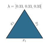
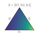
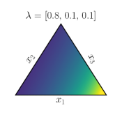
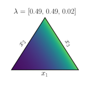
Because the CC log-likelihood is linear in the data (equation 2), the density is necessarily convex. It follows that the modes of the CC are at the extrema; example density plots are shown in figure 1. In this sense, the CC is a less flexible family than the Dirichlet, as it cannot represent interior modes. In the context of fitting a probability distribution (possibly in a regression setting) to compositional outcomes, however, this choice prevents the CC from concentrating mass on single observations, a fundamental tradeoff with the Dirichlet distribution and other transformation-based competitors such as Aitchison (1982, 1994, 1999). The mode of the CC is the basis vector associated with the index of the data, provided the maximizer is unique.

3.2 Concentration of mass
The CC exhibits very different concentration of mass at the extrema relative to the Dirichlet. The former is always finite and strictly positive, whereas the latter either diverges or vanishes for almost all parameter values, in other words:
| (3) |
The important distinction lies at the limit points; the CC is supported on the closed simplex, whereas the Dirichlet and its transformation-based alternatives are defined only on its interior. Thus, the CC log-likelihood can automatically model data with zeros, without requiring specialized techniques such as Palarea-Albaladejo & Martín-Fernández (2008); Scealy & Welsh (2011); Stewart & Field (2011); Tsagris & Stewart (2018); Hijazi et al. (2011), to name but a few. The sheer amount of published work dedicated to this long-standing issue should convince the reader that this property of the CC distribution provides a substantial advantage in an applied modeling context.
3.3 Exponential Family
The CC defines an exponential family of distributions; noting that by definition , we can rewrite equation 2:
| (4) |
Letting , so that , gives the natural parameter of our exponential family. Under this parameterization, we can ignore the th component, , and our parameter space becomes the unrestricted , which is more convenient for optimization purposes and will be used throughout our implementation. With a slight abuse of notation,333We will write and interchangeably depending on context, and similarly for the density functions and . our density simplifies to:
| (5) |
This last formulation makes it apparent that, under a CC likelihood, the mean of the data is minimal sufficient. By the standard theory of exponential families, this implies that the MLE of the CC distribution will produce an unbiased estimator of the mean parameter. To be precise, if maximizes the CC likelihood, and is the corresponding mean parameter obtained from , then , where is the empirical average of the data. Thus, the CC MLE is unbiased for the true mean, irrespective of the data-generating distribution.
This fact stands in contrast to the Dirichlet, in which the sufficient statistic is the mean of the logarithms, or other competitors, in which less can be said about the bias, partly as a result of their added complexities. Not only are these biases undesirable at a philosophical level, but we will also find in section 5 that, empirically, they compromise the performance of the Dirichlet relative to the CC.
3.4 Normalizing constant
For our new distribution to be of practical use, we must first derive its normalizing constant, which we denote by , defined by the equation:
| (6) |
where is the Lebesgue measure.
Proposition. The normalizing constant of a random variable is given by:
| (7) |
provided for all .
Proof. We present a proof by induction in section A of the supplementary material.
Note it is only on a set of Lebesgue measure zero that for some , and while the CC is still properly defined in these cases, the normalizing constant takes a different form. However, evaluating equation 7 when two (or more) parameters are approximately equal can result in numerical instability. In our experiments (§5), the limited instances of this issue were dealt with by zeroing out any error-inducing gradients during optimization.
It may come as a surprise that the normalizing constant of the CC distribution (7) admits a simple closed form expression in terms of elementary functions; the same cannot be said of almost any multivariable function that one might hope to integrate over the simplex (compare to the Dirichlet density, which integrates to a product of gamma functions). Thus, the CC turns out to be a very natural choice for a distribution on this sample space, which has not been previously proposed in the literature. The appeal of equation 7 is not just theoretical; it allows the CC log-likelihood to be optimized straightforwardly using automatic differentiation. In other words, not only is the CC distribution able to address several key limitations of the Dirichlet, but it does so without sacrificing mathematical simplicity (the form of the densities are very similar) or exponential family properties, or adding additional model parameters.
3.5 Mean and variance
By the standard theory of exponential families, the mean and covariance of the CC distribution can be computed by differentiating the normalizing constant. Thus, while cumbersome to write down analytically, we can evaluate these quantities using automatic differentiation. Higher moments, including skewness and kurtosis, can also be derived from the normalizing constant, as well as a number of other distributional results, such as the characteristic function or KL divergence (see section B from the supplementary material).
3.6 Related distributions
The Dirichlet distribution can be thought of as a generalization of the beta distribution to higher dimensions, which arises by taking the product of independent beta densities and restricting the resulting function to the simplex. In the same way, the CC provides a multivariate extension of the recently proposed continuous Bernoulli (CB) distribution (Loaiza-Ganem & Cunningham, 2019), which is defined on by:
| (8) |
First, observe that this density is equivalent to the univariate case of the CC (i.e. ). Second, note that the full CC density (2) corresponds to the product of independent CB densities, restricted to the simplex, an idea that we will capitalize on when designing sampling algorithms for the CC (§4). In this sense, the beta, Dirichlet, CB and CC distributions form an intimately connected tetrad; the CB and the CC switch the role of the parameter and the variable in the beta and Dirichlet densities, respectively, and the Dirichlet and CC extend to the simplex the product of beta and CB densities, respectively. The analogy to the beta and CB families is not just theoretical; the CB arose in the context of Variational Autoencoders (Kingma & Welling, 2014) and showed empirical improvements over the beta for modeling data which lies close to the extrema of the unit interval (Loaiza-Ganem & Cunningham, 2019). Similarly, the CC provides theoretical and empirical improvements over the Dirichlet for modeling extremal data (§3.2, 5).
4 Sampling
Sampling is of fundamental importance for any probability distribution. We developed two novel sampling schemes for the CC, which we highlight here; full derivations and a study of their performance (including reparameterization gradients) can be found in the supplement (section C). We note that, while the Dirichlet distribution can be sampled efficiently via normalized gamma draws or stick-breaking (Connor & Mosimann, 1969), we are not aware of any such equivalents for the CC (see section B.4 of the supplement).
Given the relationship between the CB and the CC densities (§3.6), a naive rejection sampler for the CC follows directly by combining independent CB draws (using the closed form inverse cdf), and accepting only those that fall on the simplex. This basic sampler scales poorly in . We improve upon it via a reordering operation, resulting in vastly better performance (see section C.2 and figure 1 from the supplement). The central concept of this scheme is to sort the parameter and reject as soon as samples leave the simplex; this sampler is outlined in algorithm 1.
Input: target distribution .
Output: sample drawn from target.
Algorithm 1 performs particularly well in the case that is unbalanced, with a small number of components concentrating most of the mass. However, its efficiency degrades under balanced configurations of ; this shortcoming motivates the need for our second sampler (algorithm 2), which performs particularly well in the balanced setting. Conceptually, this second sampler will exploit a permutation-induced partition of the unit cube into simplices, combined with a relaxation of the CC which is invariant under permutations, and can be mapped back to the original CC distribution.
At a technical level, first note that if is a permutation of and , then we can (almost, in the measure-theoretic sense) partition where the union is over all permutations. Second, we can generalize the CC to an arbitrary sample space by writing . By the change of variable formula, we note that this family is invariant to invertible linear maps in the sense that, if and , where is an invertible matrix, then , where . Hence, if is a lower-triangular matrix of ones and denotes the identity permutation, then , and it follows that we can sample from by sampling and transforming with . Conveniently, can be sampled by first drawing a -valued vector of independent CB variates, namely , then transforming into by applying , where is the permutation matrix that orders the elements of , and finally accepting with probability:
| (9) |
where is the rejection sampling constant:
| (10) |
This sampling scheme is shown altogether in algorithm 2. It performs particularly well in the case that is balanced, since the distributions induced on by and the permutations thereof, are similar, resulting in high acceptance probabilities. Taken together with algorithm 1, our permutation sampler provides an efficient, theoretically understood, and reparameterizable sampling scheme for the CC.
Input: target distribution .
Output: sample drawn from target.
5 Experiments
5.1 Simulation study
We begin our experiments with a simulation study that illustrates the biases incurred from fitting Dirichlet distributions to compositional data. Our procedure is as follows:
-
1.
Fix a ground-truth distribution on the simplex. This will either be a Dirichlet where the (known) parameter value is drawn from independent variates, or a CC where the (known) parameter value is sampled uniformly on the simplex.
-
2.
Fix a sample size . This will range from to .
-
3.
In each of one million trials, draw a sample of i.i.d. observations .
-
4.
Use the samples to compute one million MLEs for the mean parameter, under both a Dirichlet and a CC likelihood.
-
5.
Average the one million MLEs and subtract the true mean to obtain estimates of the ‘empirical bias’.
-
6.
Repeat the steps for different values of , , and , as prescribed.
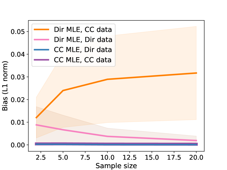
The results of this experiment are shown in figure 2. As we already knew from the theory of exponential families, only the CC estimator is unbiased. The Dirichlet estimator is, at best, asymptotically unbiased, and only in the unrealistic setting of a true Dirichlet generative process (pink line). It is worth emphasizing that, even in this most-favorable case for the Dirichlet, the CC outperforms (pink line versus blue line). The error bars show standard deviation over different draws from the prior distribution of step 1. The large error bars on the Dirichlet, especially under non-Dirichlet data (orange line) indicate that its bias is highly sensitive to the true mean of the distribution, reaching up to several percentage points (relative to the unit-sum total), whereas the CC is unbiased across the board. Lastly, note that while a sample size of 20 may seem small in the context of machine learning, this is in fact reasonable in terms of the ratio of observations to parameters, as larger samples typically call for more flexible models.
5.2 UK election data
We next consider a real-world example from the 2019 UK general election (Uberoi et al., 2019). The UK electorate is divided into 650 constituencies, each of which elects 1 member of parliament (MP) in a winner-takes-all vote. Typically, each of the major parties will be represented in each constituency, and will win a share of that constituency’s electorate. Thus, our data consists of 650 observations444We split the data into an 80/20 training and test set at random., each of which is a vector of proportions over the four major parties (plus a fifth proportion for a ‘remainder’ category, which groups together smaller parties and independent candidates). We regress this outcome on four predictors: the region of the constituency (a categorical variable with 4 levels), an urban/rural indicator, the size of the constituency’s electorate, and the voter turnout percentage from the previous general election. While there is a host of demographic data that could be used to construct increasingly more informative predictors here, we stick to the reduced number of variables that were available in our original dataset, as the goal of our analysis is not to build a strong predictive model, but rather to illustrate the advantages and disadvantages of using the novel CC distribution as opposed to the Dirichlet. For the benefit of the latter, since our data contains zeros (not all major parties are represented in all constituencies), we add an insignificant share to all observations and re-normalize prior to modeling (without this data distortion, the Dirichlet would fail even more grievously).
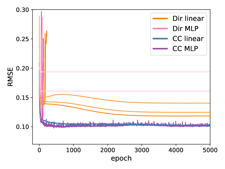
We fit regression networks to this data with two different loss functions, one where we assume the response follows a Dirichlet likelihood (Campbell & Mosimann, 1987; Hijazi, 2003; Hijazi & Jernigan, 2009), the other with our own CC likelihood instead. We first fit the simplest linear version: for the Dirichlet, we map the inputs into the space of by applying a single single linear transformation followed by an activation function; for the CC, a single linear transformation is sufficient to map the inputs to the unconstrained space of (in statistical terminology, this corresponds to a generalized linear model with canonical link). Secondly, we extend our linear model to a more flexible neural network by adding a hidden layer with 20 units and ReLU activations. We train both models using Adam (Kingma & Ba, 2015).
| MAE | RMSE | ms/epoch | |
|---|---|---|---|
| Dir linear | 0.105 | 0.132 | 4 |
| CC linear | 0.075 | 0.101 | 8 |
| \hdashline[0.5pt/5pt] Dir MLP | 0.087 | 0.112 | 20 |
| CC MLP | 0.072 | 0.097 | 35 |
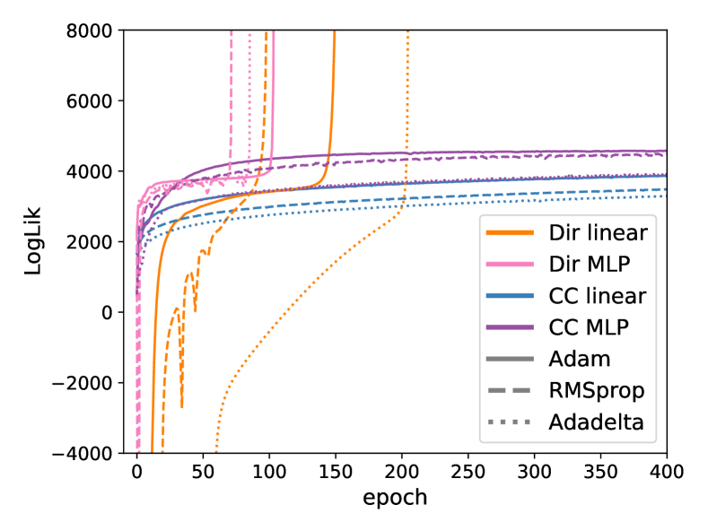
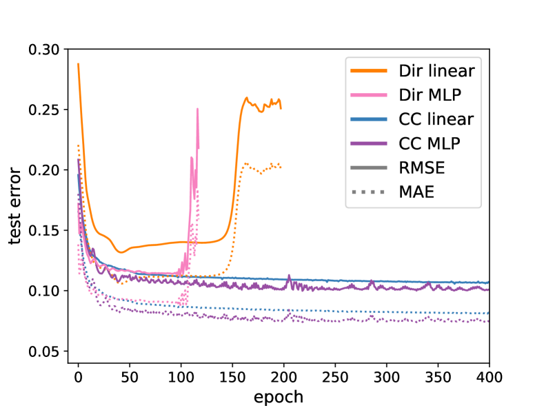
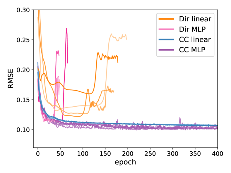
The CC models achieve better test error, with gains ranging between % and % in the and sense, as shown in table 1 and figure 3.555The and metrics are used for illustration purposes. One could, of course, optimize these metrics directly, however this would either jeopardize the probabilistic interpretation and statistical rigor of the model, or require the addition of an intractable normalizing constant to the log-likelihood. Moreover, the CC reliably converges to a performant model (which in the linear case corresponds to the MLE), whereas the Dirichlet likelihood diverges along a highly variable path in the parameter space that correspond to suboptimal models. We verify also that this behavior happens irrespective of the optimizer used to train the model (figure 4), and is consistent across random initializations of the model parameters (figure 5). Note that the Dirichlet MLP diverges faster than its linear counterpart, likely because the increased flexibility afforded by the MLP architecture allows it to place a spike on a training point more quickly.
Naturally, one might ask whether the unstable behavior of the Dirichlet can be fixed through regularization, as a suitable penalty term might be able to counterbalance the detrimental flexibility of the distribution. We test this hypothesis empirically by adding an penalty (applied to the weights and biases of the regression network) to the objective, with a varying coefficient to control the regularization strength. The results are shown in figure 6; while strong regularization does stabilize the Dirichlet, it is still unable to outperform the (unregularized) CC and it is slower to converge.
In terms of runtime, we find that the computational cost of the CC and Dirichlet gradients are of the same order of magnitude (table 1). While the CC models are slower per gradient step, they are able to find better regression functions in fewer steps. What’s more, the comparison is somewhat unfair to the CC, as the Dirichlet gradients exploit specialized numerical techniques for evaluating the digamma function that have been years in the making, whereas the same is not yet true for our novel distribution.
5.3 Model compression
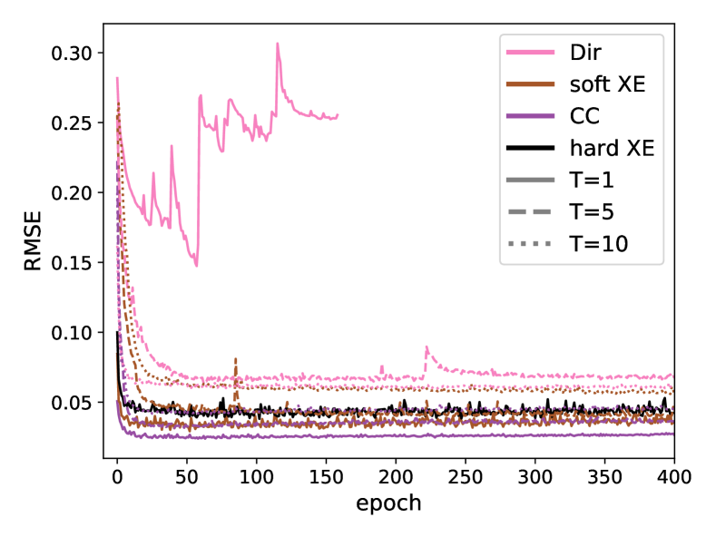
Our last experiment considers a typical model compression task (Buciluǎ et al., 2006; Ba & Caruana, 2014; Hinton et al., 2015), where we have access to an accurate ‘teacher’ model that is expensive to evaluate, which we use in order to train a cheaper ‘student’ model, typically a neural network with few layers. By training the student network to predict the fitted values of the teacher model, it can achieve better generalization than when trained on the original labels, as was shown by Buciluǎ et al. (2006); Ba & Caruana (2014); Hinton et al. (2015). These fitted values provide ‘soft targets’ that are typically located close to the extrema of the simplex, though we can also bring them towards the centroid while conserving their relative order by varying the temperature, , of the final softmax (Hinton et al., 2015).
We build on the MNIST experiment of Hinton et al. (2015); we first train a teacher neural net with two hidden layers of 1200 units and ReLU activations, regularized using batch normalization, and we use its fitted values to train smaller student networks with a single hidden layer of 30 units. We fit the student networks to the soft targets using the categorical cross-entropy (XE) loss, as well as a Dirichlet (as per Sadowski & Baldi (2018)) and a CC log-likelihood. The latter is equivalent to adding the appropriate normalization constant to the XE, thus giving a correct probabilistic interpretation to the procedure. Note that the XE and the CC objective result in the same estimator at optimality: the empirical mean of the data (we know this is true theoretically from section 3.3). However, the two objectives define different optimization landscapes, so the question of which one to use becomes an empirical one.
In this case, we found that using the CC objective leads to a lower misclassification rate on the test set than the XE (table 2), as well as a lower RMSE (measured against the soft targets outputted by the trained teacher model when evaluated on the test set), and did so consistently across temperatures (figure 7). Both the CC and XE objectives worked substantially better than the Dirichlet likelihood, and better than training the same architecture on the original hard labels. Note also that the Dirichlet performs very poorly and is unstable in the unadjusted temperature setting (), as the soft targets are very extremal and lead to numerical overflow, but performs much better at high temperatures.
| Objective | Accuracy | RMSE | s/epoch |
|---|---|---|---|
| Dirichlet | 90.6% | 0.041 | 0.9 |
| Soft XE | 94.9% | 0.029 | 0.8 |
| CC | 95.6% | 0.024 | 2.2 |
| \hdashline[0.5pt/5pt] Hard XE | 93.2% | – | 0.8 |
5.4 Latent variable models
While we have demonstrated empirical improvements from using the CC to model compositional outcomes, so far we have not found similar gains when using the CC to model latent variables, for example, in mixed-membership models such as LDA (Blei et al., 2003; Pritchard et al., 2000). Training a ‘Latent-CC-Allocation’ topic model on a corpus of 2,000 NeurIPS papers gave similar learned topics and held-out perplexities as vanilla LDA (562 vs 557 per word, respectively). However, while the Dirichlet is the conjugate prior for the multinomial, a CC prior with a multinomial likelihood leads to an intractable posterior, complicating optimization (which, in this case, is enabled by means of our sampling and reparameterization algorithms from appendix C). We note also that the CC does not share the sparsity-inducing properties of the Dirichlet, nor can it approximate the categorical distribution arbitrarily well, unlike other continuous relaxations that have been proposed in the literature (Jang et al., 2016; Maddison et al., 2016; Potapczynski et al., 2019). Nevertheless, given the widespread use of simplex-valued latent variables in probabilistic generative models, the use of the CC distribution in this context remains an open question.
6 Conclusion
Our results demonstrate the theoretical and empirical benefits of the CC, which should hold across a range of applied modeling contexts. To conclude, we summarize the main contributions of our work:
-
•
We have introduced the CC distribution, a novel exponential family defined on the simplex, that resolves a number of long-standing limitations of previous models of compositional data.
-
•
We have fully characterized our distribution and discussed its theoretical properties. Of particular importance is the sufficient statistic, which guarantees unbiased estimators, and the favorable behavior of the log-likelihood, which leads to ease of optimization and robustness to extreme values.
-
•
Empirically, the CC defines probabilistic models that outperform their Dirichlet counterparts and other competitors, and allows for a rich class of regression functions, including neural networks.
-
•
We have also designed and implemented novel and efficient rejection sampling algorithms for the CC.
Taken together, these findings indicate the CC is a valuable density for probabilistic machine learning with simplex-valued data.
Acknowledgements
We thank Andres Potapczynski, Yixin Wang and the anonymous reviewers for helpful conversations, and the Simons Foundation, Sloan Foundation, McKnight Endowment Fund, NSF 1707398, and the Gatsby Charitable Foundation for support.
References
- Aitchison (1982) Aitchison, J. The statistical analysis of compositional data. Journal of the Royal Statistical Society: Series B (Methodological), 44(2):139–160, 1982.
- Aitchison (1994) Aitchison, J. Principles of compositional data analysis. Lecture Notes-Monograph Series, 24:73–81, 1994. ISSN 07492170.
- Aitchison (1999) Aitchison, J. Logratios and natural laws in compositional data analysis. Mathematical Geology, 31(5):563–580, 1999.
- Avalos et al. (2018) Avalos, M., Nock, R., Ong, C. S., Rouar, J., and Sun, K. Representation learning of compositional data. In Advances in Neural Information Processing Systems, pp. 6679–6689, 2018.
- Ba & Caruana (2014) Ba, J. and Caruana, R. Do deep nets really need to be deep? In Advances in neural information processing systems, pp. 2654–2662, 2014.
- Barnard et al. (2003) Barnard, K., Duygulu, P., Forsyth, D., Freitas, N. d., Blei, D. M., and Jordan, M. I. Matching words and pictures. Journal of machine learning research, 3(Feb):1107–1135, 2003.
- Blei et al. (2003) Blei, D. M., Ng, A. Y., and Jordan, M. I. Latent dirichlet allocation. Journal of machine Learning research, 3(Jan):993–1022, 2003.
- Breunig & Busemeyer (2012) Breunig, C. and Busemeyer, M. R. Fiscal austerity and the trade-off between public investment and social spending. Journal of European Public Policy, 19(6):921–938, 2012.
- Buccianti & Pawlowsky-Glahn (2005) Buccianti, A. and Pawlowsky-Glahn, V. New perspectives on water chemistry and compositional data analysis. Mathematical Geology, 37(7):703–727, 2005.
- Buccianti et al. (2006) Buccianti, A., Mateu-Figueras, G., and Pawlowsky-Glahn, V. Compositional data analysis in the geosciences: From theory to practice. Geological Society of London, 2006.
- Buciluǎ et al. (2006) Buciluǎ, C., Caruana, R., and Niculescu-Mizil, A. Model compression. In Proceedings of the 12th ACM SIGKDD international conference on Knowledge discovery and data mining, pp. 535–541, 2006.
- Campbell & Mosimann (1987) Campbell, G. and Mosimann, J. Multivariate methods for proportional shape. In ASA Proceedings of the Section on Statistical Graphics, volume 1, pp. 10–17. Washington, 1987.
- Connor & Mosimann (1969) Connor, R. J. and Mosimann, J. E. Concepts of independence for proportions with a generalization of the dirichlet distribution. Journal of the American Statistical Association, 64(325):194–206, 1969.
- Douma & Weedon (2019) Douma, J. C. and Weedon, J. T. Analysing continuous proportions in ecology and evolution: A practical introduction to beta and dirichlet regression. Methods in Ecology and Evolution, 10(9):1412–1430, 2019.
- Egozcue et al. (2003) Egozcue, J. J., Pawlowsky-Glahn, V., Mateu-Figueras, G., and Barcelo-Vidal, C. Isometric logratio transformations for compositional data analysis. Mathematical Geology, 35(3):279–300, 2003.
- Erosheva (2002) Erosheva, E. A. Grade of membership and latent structure models with application to disability survey data. PhD thesis, PhD thesis, Carnegie Mellon University, Department of Statistics, 2002.
- Filzmoser et al. (2009) Filzmoser, P., Hron, K., and Reimann, C. Univariate statistical analysis of environmental (compositional) data: problems and possibilities. Science of the Total Environment, 407(23):6100–6108, 2009.
- Fry et al. (2000) Fry, J. M., Fry, T. R., and McLaren, K. R. Compositional data analysis and zeros in micro data. Applied Economics, 32(8):953–959, 2000.
- Gloor et al. (2017) Gloor, G. B., Macklaim, J. M., Pawlowsky-Glahn, V., and Egozcue, J. J. Microbiome datasets are compositional: and this is not optional. Frontiers in microbiology, 8:2224, 2017.
- Gueorguieva et al. (2008) Gueorguieva, R., Rosenheck, R., and Zelterman, D. Dirichlet component regression and its applications to psychiatric data. Computational statistics & data analysis, 52(12):5344–5355, 2008.
- Hijazi et al. (2011) Hijazi, R. et al. An em-algorithm based method to deal with rounded zeros in compositional data under dirichlet models. 2011.
- Hijazi (2003) Hijazi, R. H. Analysis of compositional data using Dirichlet covariate models. PhD thesis, American University, 2003.
- Hijazi & Jernigan (2009) Hijazi, R. H. and Jernigan, R. W. Modelling compositional data using dirichlet regression models. Journal of Applied Probability & Statistics, 4(1):77–91, 2009.
- Hinton et al. (2015) Hinton, G., Vinyals, O., and Dean, J. Distilling the knowledge in a neural network. In NIPS Deep Learning and Representation Learning Workshop, 2015.
- Jang et al. (2016) Jang, E., Gu, S., and Poole, B. Categorical reparameterization with gumbel-softmax. arXiv preprint arXiv:1611.01144, 2016.
- Katz & King (1999) Katz, J. N. and King, G. A statistical model for multiparty electoral data. American Political Science Review, 93(1):15–32, 1999.
- Kingma & Ba (2015) Kingma, D. P. and Ba, J. Adam: A method for stochastic optimization. In 3rd International Conference on Learning Representations, ICLR 2015, San Diego, CA, USA, May 7-9, 2015, Conference Track Proceedings, 2015.
- Kingma & Welling (2014) Kingma, D. P. and Welling, M. Auto-encoding variational bayes. In 2nd International Conference on Learning Representations, ICLR 2014, Banff, AB, Canada, April 14-16, 2014, Conference Track Proceedings, 2014.
- Loaiza-Ganem & Cunningham (2019) Loaiza-Ganem, G. and Cunningham, J. P. The continuous bernoulli: fixing a pervasive error in variational autoencoders. In Advances in Neural Information Processing Systems, pp. 13266–13276, 2019.
- Ma et al. (2016) Ma, Z., Xue, J.-H., Leijon, A., Tan, Z.-H., Yang, Z., and Guo, J. Decorrelation of neutral vector variables: Theory and applications. IEEE transactions on neural networks and learning systems, 29(1):129–143, 2016.
- Maddison et al. (2016) Maddison, C. J., Mnih, A., and Teh, Y. W. The concrete distribution: A continuous relaxation of discrete random variables. arXiv preprint arXiv:1611.00712, 2016.
- Masoudimansour & Bouguila (2017) Masoudimansour, W. and Bouguila, N. Dirichlet mixture matching projection for supervised linear dimensionality reduction of proportional data. In 2017 IEEE International Conference on Acoustics, Speech and Signal Processing (ICASSP), pp. 2806–2810. IEEE, 2017.
- Na et al. (2014) Na, J. H., Demetriou, M. D., Floyd, M., Hoff, A., Garrett, G. R., and Johnson, W. L. Compositional landscape for glass formation in metal alloys. Proceedings of the National Academy of Sciences, 111(25):9031–9036, 2014.
- Ng et al. (2011) Ng, K. W., Tian, G.-L., and Tang, M.-L. Dirichlet and related distributions: Theory, methods and applications, volume 888. John Wiley & Sons, 2011.
- Palarea-Albaladejo & Martín-Fernández (2008) Palarea-Albaladejo, J. and Martín-Fernández, J. A modified em alr-algorithm for replacing rounded zeros in compositional data sets. Computers & Geosciences, 34(8):902–917, 2008.
- Parisotto et al. (2015) Parisotto, E., Ba, J. L., and Salakhutdinov, R. Actor-mimic: Deep multitask and transfer reinforcement learning. arXiv preprint arXiv:1511.06342, 2015.
- Pawlowsky-Glahn & Buccianti (2011) Pawlowsky-Glahn, V. and Buccianti, A. Compositional data analysis. Wiley Online Library, 2011.
- Pawlowsky-Glahn & Egozcue (2006) Pawlowsky-Glahn, V. and Egozcue, J. J. Compositional data and their analysis: an introduction. Geological Society, London, Special Publications, 264(1):1–10, 2006.
- Pawlowsky-Glahn & Olea (2004) Pawlowsky-Glahn, V. and Olea, R. A. Geostatistical analysis of compositional data, volume 7. Oxford University Press, 2004.
- Pawlowsky-Glahn et al. (2015) Pawlowsky-Glahn, V., Egozcue, J. J., and Tolosana-Delgado, R. Modeling and analysis of compositional data. John Wiley & Sons, 2015.
- Potapczynski et al. (2019) Potapczynski, A., Loaiza-Ganem, G., and Cunningham, J. P. Invertible gaussian reparameterization: Revisiting the gumbel-softmax. arXiv preprint arXiv:1912.09588, 2019.
- Pritchard et al. (2000) Pritchard, J. K., Stephens, M., and Donnelly, P. Inference of population structure using multilocus genotype data. Genetics, 155(2):945–959, 2000.
- Quinn et al. (2018) Quinn, T. P., Erb, I., Richardson, M. F., and Crowley, T. M. Understanding sequencing data as compositions: an outlook and review. Bioinformatics, 34(16):2870–2878, 2018.
- Sadowski & Baldi (2018) Sadowski, P. and Baldi, P. Neural network regression with beta, dirichlet, and dirichlet-multinomial outputs. 2018.
- Scealy & Welsh (2011) Scealy, J. and Welsh, A. Regression for compositional data by using distributions defined on the hypersphere. Journal of the Royal Statistical Society: Series B (Statistical Methodology), 73(3):351–375, 2011.
- Stewart & Field (2011) Stewart, C. and Field, C. Managing the essential zeros in quantitative fatty acid signature analysis. Journal of Agricultural, Biological, and Environmental Statistics, 16(1):45–69, 2011.
- Tsagris & Stewart (2018) Tsagris, M. and Stewart, C. A dirichlet regression model for compositional data with zeros. Lobachevskii Journal of Mathematics, 39(3):398–412, 2018.
- Tzeng et al. (2015) Tzeng, E., Hoffman, J., Darrell, T., and Saenko, K. Simultaneous deep transfer across domains and tasks. In Proceedings of the IEEE International Conference on Computer Vision, pp. 4068–4076, 2015.
- Uberoi et al. (2019) Uberoi, E., Baker, C., and Cracknell, R. General election 2019: Full results and analysis. Parliament UK. July, 2019.
- Wang et al. (2008) Wang, H.-Y., Yang, Q., Qin, H., and Zha, H. Dirichlet component analysis: feature extraction for compositional data. In Proceedings of the 25th international conference on Machine learning, pp. 1128–1135. ACM, 2008.