When Less Is More: Systematic Analysis of Cascade-Based Community Detection
Abstract.
Information diffusion, spreading of infectious diseases, and spreading of rumors are fundamental processes occurring in real-life networks. In many practical cases, one can observe when nodes become infected, but the underlying network, over which a contagion or information propagates, is hidden. Inferring properties of the underlying network is important since these properties can be used for constraining infections, forecasting, viral marketing, and so on. Moreover, for many applications, it is sufficient to recover only coarse high-level properties of this network rather than all its edges. This article conducts a systematic and extensive analysis of the following problem: Given only the infection times, find communities of highly interconnected nodes. This task significantly differs from the well-studied community detection problem since we do not observe a graph to be clustered. We carry out a thorough comparison between existing and new approaches on several large datasets and cover methodological challenges specific to this problem. One of the main conclusions is that the most stable performance and the most significant improvement on the current state-of-the-art are achieved by our proposed simple heuristic approaches agnostic to a particular graph structure and epidemic model. We also show that some well-known community detection algorithms can be enhanced by including edge weights based on the cascade data.
1. Introduction
Many social, biological, and information systems can be represented by networks whose nodes are items, and links are relations between them. In recent years, there has been a great deal of interest in analyzing propagation processes arising on such network structures. Examples of such processes are spreading of infectious diseases (Hufnagel et al., 2004) and computer viruses (Wang et al., 2000), promotion of products via viral marketing (Kempe et al., 2003), propagation of information (Romero et al., 2011), opinion dynamics (Noorazar, 2020), and so on. Usually, a contagion appears at some network node and then spreads to other nodes over the network’s edges. In many practical scenarios, one can observe when nodes become infected, but the underlying network is hidden. For instance, during an epidemic, a person becomes ill but cannot tell who infected them; in viral marketing, we observe when customers buy products but not who influenced their decisions. Another example is Twitter, which sells a stream of tweets to other companies, but the social graph is not disclosed; for each retweet, only information about the cascade’s root node is available. The hidden network inference problem received much attention recently (Daneshmand et al., 2014; Gomez Rodriguez et al., 2014; Gomez-Rodriguez and Schölkopf, 2012; Ramezani et al., 2017). While these articles aim at recovering the actual network connections, such detailed information may not be needed in many cases. Moreover, the unobserved network may not be unique or well defined: Users may communicate via different social networks or offline. In many practical applications, only some global properties of the network are important. For example, in viral marketing, one may wish to find the most influential users, while for recommendation systems, one may look for groups of users with similar preferences.
In this article, we analyze the problem, which recently attracted interest in the literature (Barbieri et al., 2017; Ramezani et al., 2018), of inferring community structure of a given network based solely on cascades (e.g., information or epidemic) propagating through this network. Communities are groups of highly interconnected nodes with relatively few edges joining nodes of different groups, such as groups by interests in social networks or pages on related topics on the Web (Fortunato, 2010). Discovering communities is one of the most prominent tasks in network analysis with many recent applications, for example, in anomaly detection (Ma et al., 2021), financial systems (Kukreti et al., 2020), and dynamic brain networks (Martinet et al., 2020). Compared to the traditional community detection, our work is quite different because we do not have the network available to us, we have only cascade data observed on this network. For each cascade, we observe only infected nodes and their infection timestamps. Leveraging cascade information for community detection is important, for example, for preventing the spreading of fake news (Zhou and Zafarani, 2019) and viral infections such as SARS-CoV-2 (Gösgens et al., 2021a).
The main contribution of this article is a thorough theoretical and empirical analysis of a developing area of inferring community structure based on cascade data, as stated formally in Section 3. Specifically:
-
•
We propose and analyze several new algorithms and compare them to the state-of-the-art. In particular, we consider two types of approaches: based on likelihood maximization under specific model assumptions and based on the clustering of a surrogate network (Section 4).
-
•
We propose new evaluation benchmarks (real and synthetic graphs with natural and synthetic cascades) and discuss important methodological questions on properly evaluating and comparing algorithms (Section 5).
-
•
Via extensive experiments on a variety of networks,111The source code is available at https://github.com/ostroumova-la/cascade_communities. we conclude that the most stable performance is obtained by our proposed heuristics that are agnostic to a particular graph structure and epidemic model. These heuristics outperform more advanced approaches and work equally well on different networks and epidemics of different types (Section 6).
Thus, our work significantly extends previous research on the subject: We analyze a comprehensive list of algorithms, we compare them empirically on several datasets with different cascade types, and we thoroughly discuss critical methodological aspects of the problem at hand, such as dealing with unobserved nodes, that have been overlooked in the literature.
A preliminary version of this article was presented in Prokhorenkova et al. (2019). The current article substantially extends the previous work in several important directions: (1) significantly extending and improving the experimental part by adding more datasets and more cascade models; most importantly, we add the Twitter data with real cascades and natural communities (Section 5.1); (2) adding a new surrogate-graph-based method called CosineSim (Section 4.3.3) to support our claim that comparing advanced methods with simple solutions is essential; (3) analyzing the problem of how to aggregate and compare results on several datasets of different properties and sizes (Section 5.4), which is important for a systematic analysis on various data; (4) discussing how to measure the quality of an algorithm, especially when the network is only partially observed (Section 5.3) — a very important question that may affect research conclusions; and (5) also investigating how to properly generate epidemic data for experiments (in case of not having real cascades) (Section 5.2). To sum up, this extended version provides a thorough analysis of the problem of community detection based on cascade data and discusses some methodological questions related to this task. We believe that our work would stimulate further theoretical and practical research in this area.
2. Related Work
In this section, we first discuss two topics that are closely related to our work and have been extensively studied in the literature: inferring the edges of the underlying network based on cascades and community detection in known graphs. Next, we address the state-of-the-art research on community detection from cascades, which we use as baselines.
2.1. Network Inference from Cascades
A series of recent articles addressed the following task: by observing infection (activation) times of nodes in several cascades, infer the underlying network’s edges. NetInf algorithm developed by Gomez-Rodriguez et al. (2010) is based on the maximization of the likelihood of the observed cascades under the assumption of a specific epidemic model. To make optimization feasible, for each cascade, NetInf considers only the most likely propagation tree. This algorithm was later improved by MultiTree (Gomez-Rodriguez and Schölkopf, 2012), which includes all directed trees in the optimization and has better performance if the number of cascades is small. NetRate algorithm (Gomez-Rodriguez et al., 2011) infers not only edges but also infection rates. NetRate builds on an epidemic model that is more tractable for theoretical analysis. (We describe this model in Section 3.2.) For this model, the likelihood optimization problem turns out to be convex. ConNIe algorithm (Myers and Leskovec, 2010) also uses convex optimization, with the goal of inferring transmission probabilities for all edges. In (Gomez-Rodriguez et al., 2013b; Gomez Rodriguez et al., 2014), it is additionally assumed that the underlying network is not static, and the proposed algorithm InfoPath provides estimates of the structure and temporal dynamics of the hidden network. KernelCascade (Du et al., 2012) also extends NetRate, where the authors use a less restrictive cascade model. The DANI algorithm (Ramezani et al., 2017) is interesting because it explicitly accounts for the community structure to enhance the inference of networks’ edges. There are some other recent network inference algorithms not covered here, e.g., (Hoffmann et al., 2020a) studies the methods for recovering a mixture of graphs and (Gray et al., 2020) proposes a new Bayesian method; see also references therein.
2.2. Community Detection
Another direction closely related to the current research is community detection. For an overview of classic results in this area, we refer the reader to several survey articles (Chakraborty et al., 2017; Coscia et al., 2011; Fortunato, 2010; Fortunato and Hric, 2016). Many community detection algorithms are based on optimizing modularity (Newman and Girvan, 2004), which measures the goodness of a partition for a given graph. Probably the most well-known and widely used greedy modularity optimization algorithm is Louvain (Blondel et al., 2008), which iteratively moves nodes or groups of nodes from one community to another while improving modularity. Some of the methods discussed in this article use the Louvain algorithm.
In recent years, deep learning approaches became very popular for graph analysis (Wu et al., 2020). Graph neural networks (GNNs) are especially effective for node classification and graph classification tasks. The main advantage of GNNs is their ability to naturally combine node features with graph structure. GNNs have also been applied to community detection (Su et al., 2021). Relevant to our research are works on unsupervised community detection (Lobov and Ivanov, 2019). Often, such approaches optimize soft modularity loss function. However, in the absence of node features, graph neural networks are often not superior to classic approaches.
Community detection algorithms most relevant to the current research are based on statistical inference. Such methods work as follows: we assume some random graph model parameterized by community assignments of nodes; then, for a given partition, we can compute the probability that this model generated the observed network structure (i.e., likelihood); finally, a partition providing the largest likelihood is chosen. In the literature, several possible choices of the random graph model and likelihood optimization methods were proposed. Early articles on likelihood optimization assumed stochastic block model (SBM) or planted partition model (PPM), where the probability that two nodes are connected depends only on their community assignments. Recently, a degree-corrected variant of this model was proposed (Karrer and Newman, 2011), and community detection methods based on this model were shown to have a better quality (Newman, 2016; Peixoto, 2013). In a recent article (Prokhorenkova and Tikhonov, 2019), the independent Lancichinetti–Fortunato–Radicchi (ILFR) model was proposed and analyzed. It was shown that this model gives the best fit to a variety of real-world networks in terms of maximizing the likelihood. Additionally, (Prokhorenkova and Tikhonov, 2019) extended the Louvain algorithm for optimizing any likelihood function.
Closer to the current work, (Barbieri et al., 2013a; He et al., 2021; Sattari and Zamanifar, 2018) proposed to enhance community detection algorithms by using the information about spreading cascades. However, to find clusters, the authors use both the graph and the cascades. In contrast, the crucial assumption in our work is that the graph is not observed; hence these methods cannot be applied. Another similar setting is considered in (Sanders et al., 2020). Here, it is assumed that we observe a trajectory of a Markov chain spreading on a hidden stochastic block structure; the aim is to infer the clusters. Although the motivation is similar, our task is more complicated in two aspects: (1) In (Sanders et al., 2020), the transitions of the Markov chain are defined solely by the membership in the communities, while in our work, we assume a hidden graph structure, which significantly complicates the problem. (2) We consider cascades instead of chains and, in particular, we do not know who infected whom. Recent work (Xing et al., 2021) studies analytically the problem of detecting two communities from interactions in a gossip model, where some agents never change their state. In this work, we also leverage the (binary) states of the nodes, but the gossiping protocol fundamentally differs from cascades, and the assumption of two communities is too restrictive for our purposes. Finally, (Hoffmann et al., 2020b) develops a Bayesian model for community detection based on time series observed at each of the network’s nodes, without recovering the edges. However, their time series have a very different structure from the cascade data used in the current article.
2.3. Community Inference from Cascades
To the best of our knowledge, the article (Barbieri et al., 2013b) extended in (Barbieri et al., 2017) for the first time addressed the problem of community detection from cascades. In (Barbieri et al., 2013b, 2017), the cascade model includes the influence of individual nodes, and a membership level of a node in each community is inferred using the maximum-likelihood approach. The authors propose two algorithms: C-IC, which considers only participation of a node in a cascade, and C-Rate, which includes the time stamps but limits the node’s influence by its community. Recently, (Ramezani et al., 2018) proposed an alternative maximum-likelihood approach, which exploits the Markov property of the cascades. As an input, similarity scores of node pairs are computed based on their joint participation in cascades. The R-CoDi algorithm in (Ramezani et al., 2018) starts with a random partition, while D-CoDi starts with a partition obtained by DANI (Ramezani et al., 2017). We use all four mentioned algorithms as our baselines. A recent work (Suzuki and Tsugawa, 2021) addressed a follow-up problem of cascade-based community detection when the cascade data are incomplete. They conclude that hiding information on the nodes that participate in many cascades considerably reduces the quality of community detection, while hiding random or least active nodes has much smaller effects.
A recent work by Peixoto (2019) proposes to simultaneously recover edges and communities from epidemic data and shows that the detection of communities significantly increases the accuracy of graph reconstruction. Another research by Chen et al. (2014) also uses cascade data to identify (overlapping) communities. However, in contrast to the current work, they focus solely on Facebook and use more input data: post information, personal information, interpersonal relations, and so on.
3. Problem setup
3.1. General Setup
3.1.1. Cascades
We observe a set of cascades that propagate on a latent undirected network with nodes and edges. Each cascade is a record of observed node activation times, i.e., , where is a node, is its activation time in , is a size of a cascade. Note that we do not observe who infected whom.
3.1.2. Communities
We assume that is partitioned into non-overlapping communities: , , for . We expect to observe high intra-community density of edges compared to inter-community density. In our experiments, the ground truth partitions are available for all datasets (see Section 5.1). By observing only a set of cascades we want to find a partition similar to .
3.2. Cascade Models
3.2.1. SIR Model
The primary model for our experiments is a well-known Susceptible-Infected-Recovered (SIR) model (Keeling and Eames, 2005). Each node in the network can be in one of the three states: susceptible, infected, or recovered. An infected node infects its susceptible neighbors with a rate , and the infection is spread simultaneously and independently along all edges. An infected node recovers with a rate and then stops spreading infection in the network. For each cascade , we sample its infection rate from the Lomax (shifted Pareto) distribution to model a variety of cascades: There can be minor or widely circulated news, small-scale epidemics or a global outbreak, and so on. The source node of a cascade is chosen uniformly at random.
3.2.2. SI Model with Bounded Duration (SI-BD)
In some cases, the SIR model might not be tractable for theoretical analysis, so we assume a simpler diffusion model introduced in (Gomez-Rodriguez et al., 2011). In this model, just as in the SIR model, an activated node infects its neighbors after an exponentially distributed time with intensity , but there is no recovery rate. Instead, all nodes recover simultaneously at some threshold time , and the epidemic stops. For simplicity, we further assume to be fixed, but our methods allow for varying for different epidemics.
3.2.3. Community-Based SI-BD Model (C-SI-BD)
Another model that allows for a simpler theoretical analysis is based on the setting from (Sanders et al., 2020). It is assumed that the spreading does not occur over the edges of a graph but depends solely on the community structure . As before, the first node of a cascade is chosen uniformly at random. Each activated node can infect all other susceptible nodes independently after an exponentially distributed time. If a susceptible node belongs to the same community, then the infection rate is ; otherwise, it is , . Epidemic stops at time .
We want to stress a principal difference between the first two models (SIR and SI-BD) and the C-SI-BD model. C-SI-BD completely ignores the graph structure and takes into account only community assignments. Mathematically, C-SI-BD is equivalent to an SI-BD model on a complete graph, where the infection rate through the intra- and inter- community edges are and , respectively. Then, all nodes within one community are exchangeable, so that at any point of time, the cascade is completely described by the number of infected nodes in each community, and therefore one can hope to recover the community assignments when the number of cascades is large. On the other hand, SIR and SI-BD use explicit information on the structure of the underlying graph. Usually, graph edges are correlated with community assignments, while the infection rate over all edges is the same. As the number of cascades tends to infinity, one can get an asymptotically consistent estimator of the graph edges, but this might still not be sufficient to recover the communities. A well-known example of this phenomenon is the detectability threshold in the Stochastic Block Model (Decelle et al., 2011). In this setup, the quality of recovered communities might not improve beyond certain point, as the number of cascades grows. Such a setup is much more challenging but is realistic.
4. Algorithms
4.1. Background on Likelihood Maximization
Recall that denotes the activation time for node in cascade ; we often omit the index when the context is clear. Without loss of generality, for the first node of a cascade, we set . Finally, if a node is not infected during an epidemic, then we set .
Denote . The log-likelihood of the cascade for SI-BD with varying infection rates ( infects a susceptible neighbor after an exponentially distributed time with rate ) is given in (Gomez-Rodriguez et al., 2011), Equation (7). For our purposes, it is convenient to write this expression as
| (1) |
Here, we substituted a general form of the SI-BD epidemic model to the formula from (Gomez-Rodriguez et al., 2011) and took the logarithm.
The log-likelihood for all cascades is . We will next introduce a method based on maximizing under the cascade-based model.
4.2. ClustOpt
Consider the C-SI-BD model described in Section 3.2.3. Denote by the community assignment for a node . Recall that C-SI-BD is equivalent to the SI-BD model used in (Gomez-Rodriguez et al., 2011) when the latter is applied to a complete graph with if and otherwise. The log-likelihood in Equation (1) becomes
| (2) |
Note that in practice, is not known, so in the experiments, for each cascade, we set to be the time of the last infection plus the average time difference between successive infections.
We propose the following algorithm to maximize Equation (2).
-
(1)
Find initial partition ;
-
(2)
Find ;
-
(3)
For fixed , find .
Remark 1.
Algorithm 1 was initially inspired by the idea of alternated maximization. Surprisingly, our preliminary experiments have shown that repeating steps (2) and (3) multiple times does not improve the performance if we start from a good initial partition in step (1). A possible explanation is that although the maximization in Equation (2) does depend on and , it is determined to a great extent by . Therefore, we do not need and to be precise; we just need them to be good enough to find a high-quality in step (3). This is achieved when we start with a reasonable initial partition. That is why having a good initial partition is important for stable results.
Let us now discuss how the steps (1)–(3) are implemented.
Step (1):
The algorithm is initialized with some reasonable initial partition . In the current article, we propose to start from Clique(0) explained in Section 4.3.
Step (2):
Step (3):
We follow (Prokhorenkova and Tikhonov, 2019) and adapt the Louvain algorithm for the likelihood given in Equation (2) by computing the gain in obtained by moving a node from one community to another. Because of computational complexity, we consider only moving single nodes from one community to another and do not attempt to move groups of nodes or merge communities. More formally, we do the following. At the beginning, all vertices are grouped according to . Then, we iterate through all vertices: For each vertex , we compute the gain in coming from putting to the community of its neighbor and put to the community with the largest gain, as long as it is positive. We stop the process when we cannot improve by such local moves.
Remark 2.
In the preliminary version of this article (Prokhorenkova et al., 2019), a more involved algorithm called GraphOpt was presented. GraphOpt maximizes the likelihood under the SI-BD model rather than the C-SI-BD model. It uses the expectation-maximization framework assuming that the graph structure is a latent variable. This is a significantly more complicated task because the likelihood must be computed over all possible realizations of the hidden graph. While GraphOpt shows excellent results in some cases, its performance is unstable, and its time complexity is unacceptably large.
4.3. Clustering of Surrogate Graphs
This section presents simple yet effective methods that construct a surrogate graph and then cluster this graph by some community detection algorithm. We will mostly use the Louvain algorithm (Blondel et al., 2008). This method is appealing for several reasons: It is efficient, gives stable results, and does not require the number of clusters as an input (in contrast to, e.g., the spectral clustering).222We analyze the effect of a community detection algorithm on the performance of surrogate-graph-based methods by comparing the results obtained with Louvain to those obtained using another clustering algorithm, Infomap (Rosvall and Bergstrom, 2008) (see Sections 5.5, 6.4).
It is crucial that does not need to be similar to , it just needs to capture the community structure on an aggregated level. Our experiments show that clustering of often performs better than first inferring and then clustering it.
4.3.1. Path Algorithm
For each , let be a path connecting subsequently activated nodes. Then, we obtain by aggregating over all cascades. This leads to the following algorithm.
-
(1)
Construct weighted graph , where the weight of each
Find clusters in using the Louvain algorithm.
While this algorithm cannot be formally justified, it has the following motivation. Assume that is generated by the SI-BD model. Then, in Equation (1), we set if and are connected in and otherwise. So, we obtain
| (5) |
Now, for let us consider a graph with exactly edges that maximizes the probability in Equation (5). It is easy to check that is merely a path connecting subsequently activated nodes, i.e., .
4.3.2. Clique
Another approach is to include all possible edges that could participate in the cascade, weighing them by the proxy of their likelihood. Then, each cascade results in a weighted clique of size . The weights can be chosen, for example, as follows. For a cascade and two nodes , let us consider the probability . If , then, obviously, . If , then, as in (Gomez-Rodriguez et al., 2010), we assume that decreases exponentially with ; namely, where is a constant depending on . Since was infected from exactly one previous node, we must have Therefore,
| (6) |
Parameter essentially balances between paths and cliques: If is large, we mostly take into account subsequent nodes with small ; for small all pairs of nodes participated in are important.
Remark 3.
Note that we directly model without making assumptions about the distribution of . Although in Equation (6) is proportional to the exponential density function for , recall that if we assume that infection times are exponentially distributed, then a node is equally likely to get infected from any of the currently infected nodes due to the memory-less property. Furthermore, similarly to Path, this algorithm cannot be formally justified as optimization under a particular generative model. Indeed, if we assume a latent graph structure, then the expressions for the a-posteriori probabilities, given , that an edge exists, or that a node has been infected through this edge, are much more involved than the simple expression (6); see, e.g., the GraphOpt algorithm in (Prokhorenkova et al., 2019).
Clique constructs as the weighted graph with weight of given by , which, under our assumptions, is the expected number of times infections passed between and . To make Clique insensitive to the speed of epidemics, we take , where is the average time between infection times (we average over all pairs of infected nodes belonging to the same cascade). We also consider Clique(0) with , which is a natural choice for the SI-BD model because it mimics the memory-less property of exponential infection times. We noticed that Clique is not too sensitive to varying in a reasonable interval, while for too large Clique becomes very similar to Path.
-
(1)
Construct weighted graph with weight of given by ;
-
(2)
Find clusters in using the Louvain algorithm.
4.3.3. CosineSim
This algorithm is motivated by Ramezani et al. (2018), where the authors use cosine similarity to get initial similarities of nodes. Then, instead of applying the procedure from (Ramezani et al., 2018), we apply the Louvain algorithm to the obtained graph.
-
(1)
Compute ;
-
(2)
Construct as the weighted graph with weight of given by ;
-
(3)
Find clusters in using the Louvain algorithm.
4.4. Baselines
MultiTree uses the algorithm from (Gomez-Rodriguez and Schölkopf, 2012) to find an inferred graph , which is then clustered by the Louvain algorithm (Blondel et al., 2008).
We also propose Oracle as a superior benchmark for all possible network inference algorithms. Specifically, we construct a graph consisting of all edges that participated in cascades (assuming these edges are known, hence, the name Oracle). We cluster the obtained graph by the Louvain algorithm. Let us stress that we do not consider Oracle as our competitor as it uses information that is not available to other algorithms.
Finally, we used algorithms proposed for solving the same problem as in our work: C-IC and C-Rate (Barbieri et al., 2017), as well as R-CoDi and D-CoDi (Ramezani et al., 2018). We use the publicly available implementations provided by the authors.
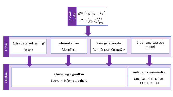
A summary of the proposed algorithms and the baselines is schematically represented in Figure 1. Stage “Edges” refers to constructions that connect the cascade data to a (possibly surrogate) network. Stage “Clusters” refers to obtaining communities.
5. Experimental Setup
5.1. Datasets
For a fair comparison of all algorithms, we performed a series of experiments using synthetic and real-world datasets.
| Dataset | ||||
|---|---|---|---|---|
| 18,470 | 2 | 29,998 | 3 |
The main dataset for our experiments is the collection of Twitter posts obtained from September till November 2010 (Conover et al., 2011). Importantly, this dataset combines both community assignments and cascades. For community assignments, Twitter users are manually classified by political alignment. The original dataset contains the following information about retweets: id of a user that started the tweet, id of a user that retweeted, the timestamp, the list of hashtags, and the number of hyperlinks included in the tweet. We processed the dataset to extract explicit cascades: Although no cascade ids are present, we assumed that a cascade can be uniquely identified by the list of hashtags, source user id, and the number of hyperlinks. Additionally, the timestamp of the first tweet is not known, so we assumed that the time difference between the original tweet and the first retweet is the same as between the first and the second retweets. This way, we obtained a dataset with about 18.5K nodes and 30K cascades. (We did not perform any further filtering.) The dataset statistics are summarized in Table 1.
The second group of datasets contains real-world networks with ground truth community assignments (see Table 2). For these datasets, we use generated epidemics (see Section 5.2) and present the results aggregated over the datasets (see Section 5.4). We include many datasets of different nature and sizes because we want to show that our conclusions generalize to different scenarios.
Finally, we also add a synthetic dataset based on the LFR model (Lancichinetti et al., 2008), which is a standard synthetic benchmark for networks with communities. This model generates graphs with power-law distributions of node degrees and cluster sizes and includes the mixing parameter , which is the fraction of inter-cluster edges. We generated a graph on 10K nodes with the power-law exponent of the degree distribution 2.5, the power-law exponent of the cluster size distribution 1.5, mixing parameter , average degree 5, maximum degree 100, and community sizes between 100 and 600. (We obtained five clusters in total.)
| Dataset | |||
|---|---|---|---|
| Karate club (Zachary, 1977) | 34 | 78 | 2 |
| Dolphins (Lusseau et al., 2003) | 62 | 159 | 2 |
| Football (Newman and Girvan, 2004) | 115 | 613 | 11 |
| Political books (Newman, 2006) | 105 | 441 | 3 |
| email-Eu-core (Leskovec et al., 2007) | 986 | 16,064 | 42 |
| Newsgroup (Yen et al., 2007) | 999 | 10,194 | 5 |
| Political blogs (Adamic and Glance, 2005) | 1,224 | 16,715 | 2 |
| Cora (McCallum et al., 2000) | 2,708 | 5,279 | 7 |
| CiteSeer (Giles et al., 1998) | 3,264 | 4,536 | 6 |
| Dataset | Lomax | |||
|---|---|---|---|---|
| Karate | 0.15 | 0.09 | 0.009 | 12 |
| Dolphins | 0.14 | 0.047 | 0.0047 | 14 |
| Football | 0.07 | 0.083 | 0.0083 | 32 |
| Pol-books | 0.08 | 0.036 | 0.0036 | 26 |
| Eu-core | 0.016 | 0.012 | 0.0012 | 230 |
| Newsgroup | 0.032 | 0.0058 | 0.00058 | 105 |
| Pol-blogs | 0.017 | 0.0024 | 0.00024 | 216 |
| Cora | 0.14 | 0.0024 | 0.00024 | 23 |
| CiteSeer | 0.21 | 0.0019 | 0.00019 | 16 |
5.2. Synthetic Cascades
For the LFR graph and the datasets described in Table 2, we generated the cascades according to all models discussed in Section 3.2. Importantly, there are both edge-based and community-based models.
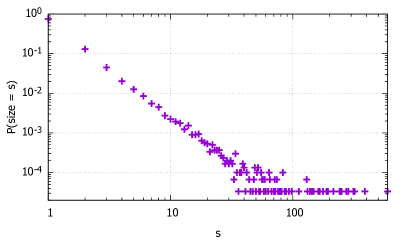
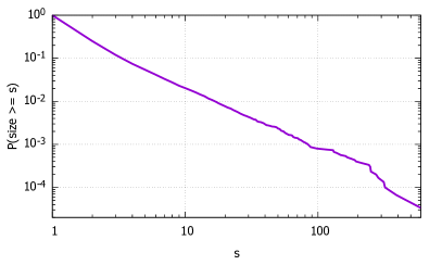
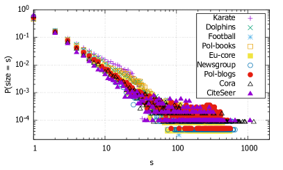
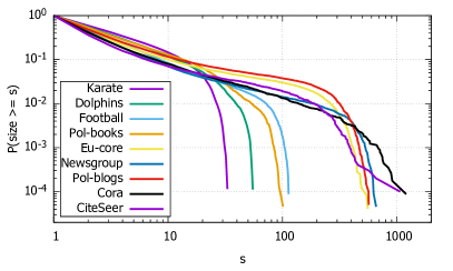
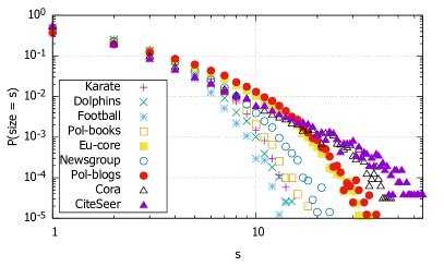
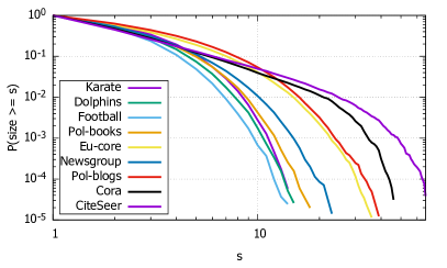
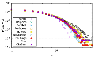
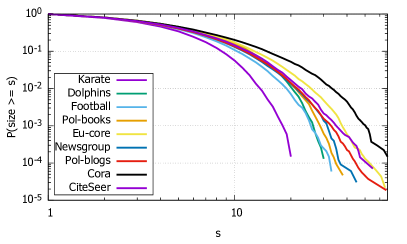
Without loss of generality, we set for the SIR model and for SI-BD and C-SI-BD. It remains to choose the parameters , , , and the parameter of the Lomax distribution used by SIR. We noticed that these parameters have to be carefully chosen to get an informative set of cascades. Otherwise, we may either get cascades consisting of single nodes or cascades consisting of almost all nodes. The following heuristics work well enough: For SIR and SI-BD, we choose parameters so that the average size of a cascade is 2; for C-SI-BD, we take and choose such that the number of cascades consisting of one node is about 20%. In Table 3, we list the parameters we used for all datasets. We plotted the obtained distributions of cascade sizes (see Figures 3–5) and checked that they are similar to those observed in the literature for real data (Bakshy et al., 2011; Galuba et al., 2010; Gomez-Rodriguez et al., 2013a; Kwak et al., 2010; Lerman et al., 2013) and for our Twitter dataset (see Figure 2).
Finally, we note that single-node cascades were removed from the generated epidemics.
5.3. Performance Measures
In this section, we discuss evaluating the quality of the obtained communities compared to the ground truth. There are many similarity indices used in the literature for the comparison of partitions. We refer to a recent work by Gösgens et al. (2021b) for a systematic study and comparison of popular indices. A critical drawback of many existing similarity measures is that they are biased with respect to cluster sizes, i.e., they prefer too small or too large clusters. For example, the Normalized Mutual Information (NMI) (Bagrow, 2008; Fortunato, 2010) is known to prefer smaller communities.
Our particular task of evaluating cascade-based community detection has some additional difficulties. Indeed, let denote the set of all nodes that participated in cascades. In many realistic scenarios, contains only a small fraction of nodes in . As a result, we obtain a partition of , which has to be compared to the ground truth partition of . There are two possible approaches to make the comparison: (1) restrict the ground truth partition only to and (2) extend the obtained partition from to , e.g., by assigning all nodes in to one cluster or individual clusters. Note that the second option has the advantage of being more interpretable (it shows how close we are to the whole ground truth partition). However, at the same time, it is vulnerable to biases: If a similarity index favors too large or too small clusters, then the assignments for the unknown set may significantly affect the obtained value.
To demonstrate the importance of choosing a proper similarity index, we perform a set of experiments comparing different choices:
-
•
Pearson correlation coefficient between the incidence vectors is an unbiased similarity index advised by Gösgens et al. (2021b).444Note that there are other good indices advised in (Gösgens et al., 2021b), e.g., the S&S index. We use the correlation coefficient as it is more widely used. Unbiased means that it does not give a preference to either large or small communities. Pearson-sub is computed only using the pairs from : We measure the Pearson correlation coefficient between the vectors of length consisting of 0s and 1s, where 1 means that two nodes belong to the same community and 0 means that they belong to different ones. Pearson-all is computed on the whole dataset: We measure the correlation between two vectors of length . For the ground truth partition, we know all entries of the vector. In contrast, for our partition, we say that if and , then the corresponding entry is 0 (different clusters), and if , then the corresponding entry is 0.5 since we do not have any information about nodes in .
- •
-
•
Jaccard index is known to be biased towards larger clusters. Jaccard-sub is computed on , and to compute Jaccard-all, we say that all unknown nodes belong to different communities (since marking them as one community would unreasonably increase the index).
-
•
F-measure (Gregory, 2008) is a harmonic average between precision and recall, where precision and recall are defined in terms of node pairs. When we compute F-measure-all, we say that all unseen nodes belong to different communities.
In most experiments, we use Pearson-sub as a primary measure since it is proven to be unbiased (Gösgens et al., 2021b). However, for the Twitter dataset, we perform a comparison of all listed measures.
5.4. Aggregating Results over Datasets
In the experiments, we compare the algorithms using all datasets from Table 2, so it is essential to be able to aggregate the obtained results so that we can compare the overall performance of algorithms over a range of datasets. Moreover, we also want to show the dependence of the performance on the number of available cascades. However, the same number of cascades (e.g., 1,000) can be sufficient to recover communities on a small dataset like Karate, while it can be far from enough to recover communities on a larger CiteSeer dataset. The following heuristic allows for balancing the data: We define a relative size of cascades as the fraction of the overall number of transmissions of infections to the number of edges in the graph. In other words, is the average number of transmissions through an edge in the graph. We empirically checked that this is a reasonable rescaling since the saturation of quality happens at similar values of for all datasets.
For a fixed value of , we average the performance over the datasets: We compute the average value of Pearson-sub and the algorithm’s average rank. To compute the latter value, for each dataset, we order all algorithms according to their performance (Pearson-sub) and obtain ranks for each algorithm; then, the obtained ranks are averaged over the datasets.
5.5. Effect of Clustering Algorithm on Surrogate-Graph-Based Methods
As discussed above, we use the Louvain method to cluster surrogate graphs. It turns out that the Louvain algorithm is well suited for clustering of surrogate graphs, and not all algorithms have this property. To show that, we compare Louvain with another well-known community detection method called Infomap (Rosvall and Bergstrom, 2008), which finds communities by minimizing the description length of random walks in the network. The results of the comparison are discussed in Section 5.5.
6. Experiments
6.1. Twitter Dataset
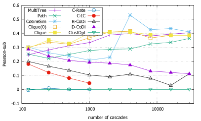
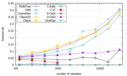
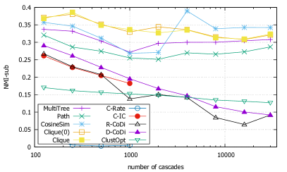
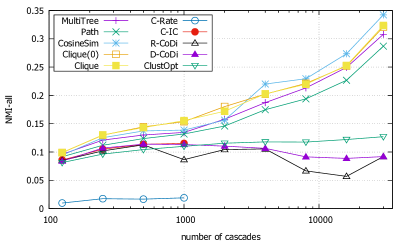
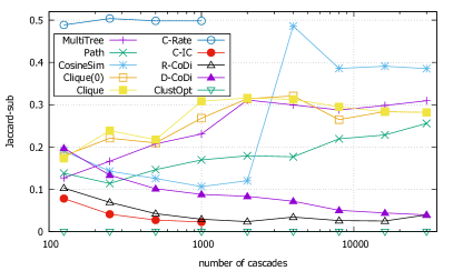
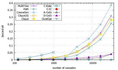
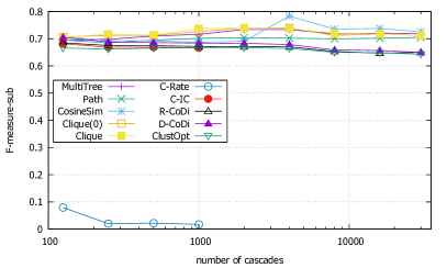
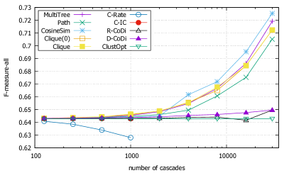
First, we compared all the algorithms on the Twitter dataset, which contains both real cascades and real community assignments; the results are presented in Figure 6.
Recall that our main performance measure is Pearson-sub (the top-left plot). First, we note that Clique algorithms are stably good for all amounts of cascade data. Further experiments will also confirm this conclusion. Also, Clique and Clique(0) have similar quality. Surprisingly, CosineSim outperforms R-CoDi and D-CoDI, i.e., Louvain algorithm above the similarity graph outperforms a more complicated algorithm presented by Ramezani et al. (2018). We guess that there can be two possible reasons for that: (1) R-CoDi and D-CoDI are based on some model assumptions and (2) these algorithms require some parameter tuning, while we used the default parameters suggested by the authors. In contrast, the Louvain algorithm is readily applied without the need for parameter tuning. For CosineSim, we also observed a phase transition when the number of epidemics is 4,000: At this point, CosineSim becomes the best one among all the algorithms. However, this transition is not observed in other experiments. We also noticed that on this dataset, MultiTree works surprisingly well, especially for large cascade sizes. However, again, this is not supported by our further experiments. Interestingly, the advanced algorithms C-IC, C-Rate, and ClustOpt have the worst performance. A possible reason is that they are strongly based on model assumptions, which may not hold for real data. Moreover, C-IC and C-Rate could not handle datasets with a large number of cascades. Concerning ClustOpt, this algorithm needs more cascade data to have a good performance, as we show by further experiments.
Now let us demonstrate the problem of proper quality evaluation as discussed in Section 5.3. In Figure 6, in addition to the primary performance measure Pearson-sub, we also show other alternatives. Recall that the measures with the postfix -all measure the quality on the same set of nodes for all cascade sizes. For a reasonable measure and a reasonable algorithm, the quality is expected to be monotone with the number of cascades. Note that with 32K cascades, -all and -sub variants coincide because this number of cascades is sufficient to cover all nodes. By further examining the measures in Figure 6, we observe huge differences between the results for different measures. These differences can be explained by the fact that some measures are biased, i.e., give a higher preference to either smaller or larger clusters. For example, the C-Rate algorithm is the best according to Jaccard, but the worst according to NMI and F-measure. This inconsistency can be explained by the fact that C-Rate produces too large communities favored by Jaccard, while F-measure and NMI are biased towards smaller clusters. Similarly, while ClustOpt has zero Pearson correlation with the target clustering, it may outperform other algorithms according to NMI just because it produces many small clusters. We conclude that it is essential to use unbiased measures. Therefore, we will continue to use the Pearson correlation coefficient in our experiments.
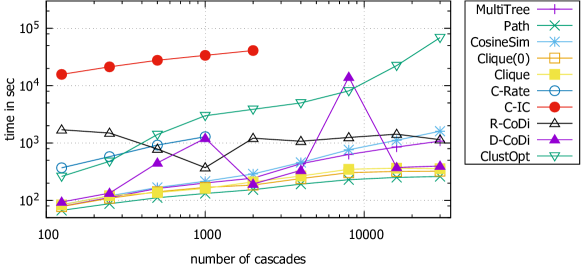
We also compared the time complexity of all the algorithms (see Figure 7). The algorithms were run on Intel(R) Xeon(R) CPU E5-2650 v2 @ 2.60 GHz. Note that this result is not an entirely fair comparison of time complexities since the algorithms are implemented via different programming languages with different levels of optimization and parallelization. Our aim is only to give an intuition about how the complexities scale with the number of cascades.
6.2. Other Real-World Datasets
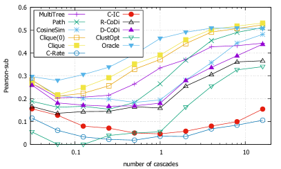
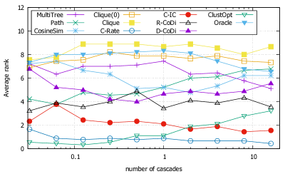
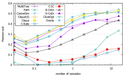
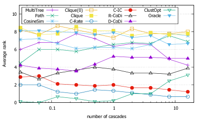
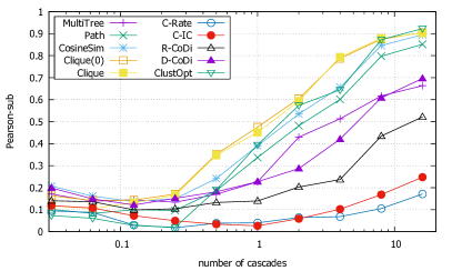
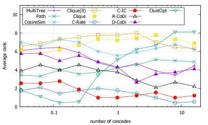
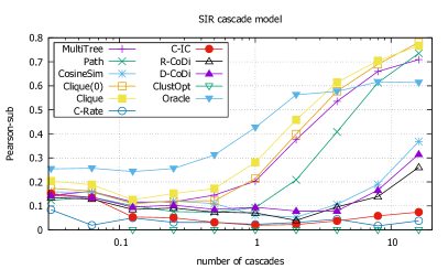
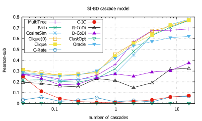
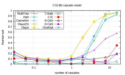
We compared all algorithms on real-world datasets listed in Table 2. Recall that for these datasets, the epidemics are synthetic and generated according to the models discussed in Section 3.2. In Figures 8–10, we plot the average Pearson-sub and the average rank, as explained in Section 5.4.
The results mostly agree with conclusions made on the Twitter dataset. Clique algorithms are the best for all sizes of cascades and all epidemic models. As before, CosineSim outperforms both R-CoDi and D-CoDI. However, there is no phase transition for CosineSim on these datasets, and for all volumes of cascade data, it is outperformed by Clique and Clique(0). Also, as we discussed above, the performance of MultiTree is not as good as on the Twitter dataset. Speaking about ClustOpt, its performance increases with the number of available cascades. ClustOpt is the best algorithm for the C-SI-BD cascade model when the number of cascades is sufficiently large, which confirms that this algorithm heavily relies on model assumptions and should be replaced by more robust algorithms when there is no evidence that the model assumptions hold.
Finally, recall that Oracle was initially considered as an upper bound for all possible network inference algorithms since it uses the exact information about who infected whom. If the number of cascades is large enough, then Oracle essentially clusters the original graph. Interestingly, in some cases, Oracle is beaten by the surrogate-graph-based algorithms, especially for a large number of cascades, although the surrogate graphs are clustered with the same Louvain algorithm. (The difference is especially apparent on the plots showing the average rank.) One can conclude that a clever weighting of edges can improve the Louvain algorithm. In other words, although Louvain is not an ideal clustering method, the effect of the errors made by Louvain is reduced by the weighting of edges provided by the surrogate-graph-based algorithms.
6.3. Synthetic Graph
The results on the synthetic LFR model are shown in Figure 11, which confirms the conclusions made previously on the real-world data. Here it is clearly seen that Clique has good and stable performance and that Oracle can be beaten by others if the number of cascades is large.
6.4. Clustering of Surrogate Graphs with Infomap
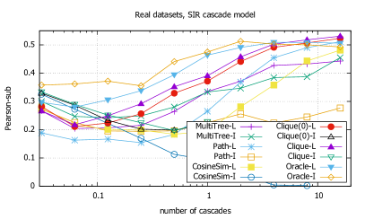
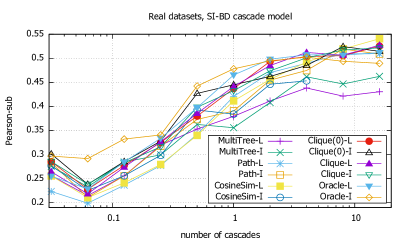
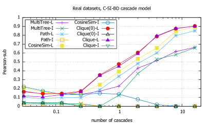
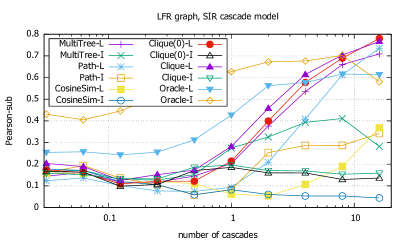
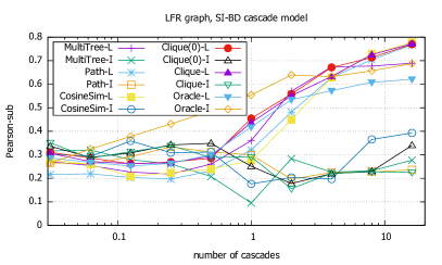
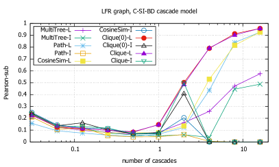
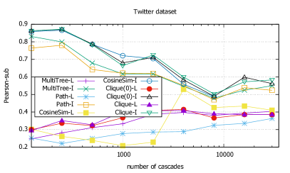
In this section, we analyze the effect of a clustering algorithm on the performance of approaches based on the clustering of surrogate graphs. In Figure 12, we compare Louvain with Infomap applied to MultiTree, Path, CosineSim, Clique, and Oracle. First, we observe that on the Twitter dataset, the results become extremely good, especially when the number of available cascades is small. However, the Clique algorithms are still among the best. In contrast, for other real datasets and for the synthetic LFR benchmark, the performance of Infomap is much worse, especially when the number of cascades is large. This holds for surrogate graphs, but not for Oracle and in some cases not for MultiTree. While analyzing this phenomenon, we noticed that for surrogate graphs, if the number of cascades is large, Infomap may predict degenerate clusterings consisting of only one cluster. This can be caused by the fact that surrogate graphs become dense when the number of cascades increases. In contrast to Infomap, Louvain is stable and works well even for dense graphs. On the other hand, on the Twitter dataset, Infomap significantly outperforms Louvain for a small number of cascades, i.e., when the density of surrogate graphs is not too large. This confirms that the choice of the clustering algorithm is essential. We conclude that Louvain leads to more stable results, but it is worth trying other options when possible.
7. Conclusion
In this article, we conducted a thorough analysis of inferring community structure based on cascade data. We compared algorithms recently proposed in the literature, simple heuristic approaches, and a more advanced approach based on mathematical modeling. Through a series of experiments on real-world and synthetic datasets, we conclude that the universal Clique method (combined with the Louvain clustering algorithm) is the best solution for the problem. This algorithm is extremely simple, efficient, and works well in all scenarios. In addition, this article covers several important methodological aspects specific to the problem at hand, e.g., choosing a performance measure to be used for comparing algorithms, aggregating results over multiple datasets, and generating realistic synthetic cascades. Another interesting conclusion is that standard clustering methods, such as the commonly used Louvain method, can be enhanced by running cascading processes on the network and weighing the node pairs based on the cascade data.
Acknowledgements.
The work of Liudmila Prokhorenkova is supported by the Ministry of Education and Science of the Russian Federation in the framework of MegaGrant 075-15-2019-1926 and by the Russian President grant supporting leading scientific schools of the Russian Federation NSh-2540.2020.1.References
- (1)
- Adamic and Glance (2005) Lada A. Adamic and Natalie Glance. 2005. The political blogosphere and the 2004 US election: Divided they blog. In Proceedings of the 3rd International Workshop on Link Discovery. ACM, 36–43.
- Bagrow (2008) James P. Bagrow. 2008. Evaluating local community methods in networks. Journal of Statistical Mechanics: Theory and Experiment 2008, 05 (2008), P05001.
- Bakshy et al. (2011) Eytan Bakshy, Jake M. Hofman, Winter A. Mason, and Duncan J. Watts. 2011. Identifying influencers on twitter. In Proceedings of the 4th ACM International Conference on Web Seach and Data Mining.
- Barbieri et al. (2013a) Nicola Barbieri, Francesco Bonchi, and Giuseppe Manco. 2013a. Cascade-based community detection. In Proceedings of the 6th ACM International Conference on Web Search and Data Mining. ACM, 33–42.
- Barbieri et al. (2013b) Nicola Barbieri, Francesco Bonchi, and Giuseppe Manco. 2013b. Influence-based network-oblivious community detection. In Proceedings of the 2013 IEEE 13th International Conference on Data Mining. IEEE, 955–960.
- Barbieri et al. (2017) Nicola Barbieri, Francesco Bonchi, and Giuseppe Manco. 2017. Efficient methods for influence-based network-oblivious community detection. ACM Transactions on Intelligent Systems and Technology 8, 2 (2017), 32.
- Blondel et al. (2008) Vincent D. Blondel, Jean-Loup Guillaume, Renaud Lambiotte, and Etienne Lefebvre. 2008. Fast unfolding of communities in large networks. Journal of Statistical Mechanics: Theory and Experiment 2008, 10 (2008), P10008.
- Chakraborty et al. (2017) Tanmoy Chakraborty, Ayushi Dalmia, Animesh Mukherjee, and Niloy Ganguly. 2017. Metrics for community analysis: A survey. ACM Computing Surveys 50, 4 (2017), 54.
- Chen et al. (2014) Yen-Liang Chen, Ching-Hao Chuang, and Yu-Ting Chiu. 2014. Community detection based on social interactions in a social network. Journal of the Association for Information Science and Technology 65, 3 (2014), 539–550.
- Conover et al. (2011) Michael D Conover, Jacob Ratkiewicz, Matthew Francisco, Bruno Gonçalves, Filippo Menczer, and Alessandro Flammini. 2011. Political polarization on twitter. In Proceedings of the 5th International AAAI Conference on Weblogs and Social Media.
- Coscia et al. (2011) Michele Coscia, Fosca Giannotti, and Dino Pedreschi. 2011. A classification for community discovery methods in complex networks. Statistical Analysis and Data Mining: The ASA Data Science Journal 4, 5 (2011), 512–546.
- Daneshmand et al. (2014) Hadi Daneshmand, Manuel Gomez-Rodriguez, Le Song, and Bernhard Schoelkopf. 2014. Estimating Diffusion Network Structures: Recovery Conditions, Sample Complexity & Soft-thresholding Algorithm. In Proceedings of the International Conference on Machine Learning. 793–801.
- Decelle et al. (2011) Aurelien Decelle, Florent Krzakala, Cristopher Moore, and Lenka Zdeborová. 2011. Asymptotic analysis of the stochastic block model for modular networks and its algorithmic applications. Physical Review E 84, 6 (2011), 066106.
- Du et al. (2012) Nan Du, Le Song, Ming Yuan, and Alex J. Smola. 2012. Learning networks of heterogeneous influence. In Proceedings of the Advances in Neural Information Processing Systems. 2780–2788.
- Fortunato (2010) Santo Fortunato. 2010. Community detection in graphs. Physics Reports 486, 3 (2010), 75–174.
- Fortunato and Hric (2016) Santo Fortunato and Darko Hric. 2016. Community detection in networks: A user guide. Physics Reports 659 (2016), 1–44.
- Galuba et al. (2010) Wojciech Galuba, Karl Aberer, Dipanjan Chakraborty, Zoran Despotovic, and Wolfgang Kellerer. 2010. Outtweeting the twitterers-predicting information cascades in microblogs. In Proceedings of the 3rd Wonference on Online social networks. ACM.
- Giles et al. (1998) C. Lee Giles, Kurt D. Bollacker, and Steve Lawrence. 1998. Citeseer: An automatic citation indexing system. In Proceedings of the 3rd ACM conference on Digital libraries. 89–98.
- Gomez-Rodriguez et al. (2011) Manuel Gomez-Rodriguez, David Balduzzi, and Bernhard Schölkopf. 2011. Uncovering the temporal dynamics of diffusion networks. In Proceedings of the 28th International Conference on Machine Learning. 561–568.
- Gomez Rodriguez et al. (2014) Manuel Gomez Rodriguez, Jure Leskovec, David Balduzzi, and Bernhard Schölkopf. 2014. Uncovering the structure and temporal dynamics of information propagation. Network Science 2, 01 (2014), 26–65.
- Gomez-Rodriguez et al. (2010) Manuel Gomez-Rodriguez, Jure Leskovec, and Andreas Krause. 2010. Inferring networks of diffusion and influence. In Proceedings of the 16th ACM SIGKDD International Conference on Knowledge Discovery and Data Mining. ACM, 1019–1028.
- Gomez-Rodriguez et al. (2013a) Manuel Gomez-Rodriguez, Jure Leskovec, and Bernhard Schölkopf. 2013a. Modeling information propagation with survival theory. In Proceedings of the International Conference on Machine Learning. 666–674.
- Gomez-Rodriguez et al. (2013b) Manuel Gomez-Rodriguez, Jure Leskovec, and Bernhard Schölkopf. 2013b. Structure and dynamics of information pathways in online media. In Proceedings of the 6th ACM International Conference on Web Search and Data Mining. ACM, 23–32.
- Gomez-Rodriguez and Schölkopf (2012) Manuel Gomez-Rodriguez and Bernhard Schölkopf. 2012. Submodular inference of diffusion networks from multiple trees. In Proceedings of the 29th International Conference on Machine Learning. 1587–1594.
- Gösgens et al. (2021a) Martijn Gösgens, Teun Hendriks, Marko Boon, Wim Steenbakkers, Hans Heesterbeek, Remco Van Der Hofstad, and Nelly Litvak. 2021a. Trade-offs between mobility restrictions and transmission of SARS-CoV-2. Journal of the Royal Society Interface 18, 175 (2021), 20200936.
- Gösgens et al. (2021b) Martijn Gösgens, Liudmila Prokhorenkova, and Alexey Tikhonov. 2021b. Systematic analysis of cluster similarity indices: How to validate validation measures. In Proceedings of the International Conference on Machine Learning.
- Gray et al. (2020) Caitlin Gray, Lewis Mitchell, and Matthew Roughan. 2020. Bayesian inference of network structure from information cascades. IEEE Transactions on Signal and Information Processing Over Networks 6 (2020), 371–381.
- Gregory (2008) Steve Gregory. 2008. A fast algorithm to find overlapping communities in networks. In Proceedings of the Joint European Conference on Machine Learning and Knowledge Discovery in Databases. Springer, 408–423.
- He et al. (2021) Ling He, Wenzhong Guo, Yuzhong Chen, Kun Guo, and Qifeng Zhuang. 2021. Discovering overlapping communities in dynamic networks based on cascade information diffusion. IEEE Transactions on Computational Social Systems (2021), 1–13.
- Hoffmann et al. (2020a) Jessica Hoffmann, Soumya Basu, Surbhi Goel, and Constantine Caramanis. 2020a. Learning mixtures of graphs from epidemic cascades. In International Conference on Machine Learning. PMLR, 4342–4352.
- Hoffmann et al. (2020b) Till Hoffmann, Leto Peel, Renaud Lambiotte, and Nick S. Jones. 2020b. Community detection in networks without observing edges. Science Advances 6, 4 (2020), eaav1478.
- Hufnagel et al. (2004) Lars Hufnagel, Dirk Brockmann, and Theo Geisel. 2004. Forecast and control of epidemics in a globalized world. Proceedings of the National Academy of Sciences of the United States of America 101, 42 (2004), 15124–15129.
- Karrer and Newman (2011) Brian Karrer and Mark E.J. Newman. 2011. Stochastic blockmodels and community structure in networks. Physical Review E 83, 1 (2011), 016107.
- Keeling and Eames (2005) Matt J. Keeling and Ken T. D. Eames. 2005. Networks and epidemic models. Journal of the Royal Society Interface 2, 4 (2005), 295–307.
- Kempe et al. (2003) David Kempe, Jon Kleinberg, and Éva Tardos. 2003. Maximizing the spread of influence through a social network. In Proceedings of the 9th ACM SIGKDD International Conference on Knowledge Discovery and Data Mining. ACM, 137–146.
- Kukreti et al. (2020) Vishwas Kukreti, Hirdesh K Pharasi, Priya Gupta, and Sunil Kumar. 2020. A perspective on correlation-based financial networks and entropy measures. Frontiers in Physics 8 (2020), 323.
- Kwak et al. (2010) Haewoon Kwak, Changhyun Lee, Hosung Park, and Sue Moon. 2010. What is Twitter, a social network or a news media?. In Proceedings of the 19th International Conference on World Wide Web. ACM, 591–600.
- Lancichinetti et al. (2008) Andrea Lancichinetti, Santo Fortunato, and Filippo Radicchi. 2008. Benchmark graphs for testing community detection algorithms. Physical Review E 78, 4 (2008), 046110.
- Lerman et al. (2013) Kristina Lerman, Rumi Ghosh, and Tawan Surachawala. 2013. Social contagion: An empirical study of information spread on Digg and Twitter follower graphs. arXiv preprint arXiv:1202.3162 (2013).
- Leskovec et al. (2007) Jure Leskovec, Jon Kleinberg, and Christos Faloutsos. 2007. Graph evolution: Densification and shrinking diameters. ACM Transactions on Knowledge Discovery from Data 1, 1 (2007), 2.
- Lobov and Ivanov (2019) Ivan Lobov and Sergey Ivanov. 2019. Unsupervised community detection with modularity-based attention model. arXiv preprint arXiv:1905.10350 (2019).
- Lusseau et al. (2003) David Lusseau, Karsten Schneider, Oliver J. Boisseau, Patti Haase, Elisabeth Slooten, and Steve M Dawson. 2003. The bottlenose dolphin community of doubtful sound features a large proportion of long-lasting associations. Behavioral Ecology and Sociobiology 54, 4 (2003), 396–405.
- Ma et al. (2021) Xiaoxiao Ma, Jia Wu, Shan Xue, Jian Yang, Chuan Zhou, Quan Z Sheng, Hui Xiong, and Leman Akoglu. 2021. A comprehensive survey on graph anomaly detection with deep learning. IEEE Transactions on Knowledge and Data Engineering (2021).
- Martinet et al. (2020) L.-E. Martinet, M. A. Kramer, W. Viles, L. N. Perkins, E. Spencer, C. J. Chu, S. S. Cash, and E. D. Kolaczyk. 2020. Robust dynamic community detection with applications to human brain functional networks. Nature Communications 11, 1 (2020), 1–13.
- McCallum et al. (2000) Andrew Kachites McCallum, Kamal Nigam, Jason Rennie, and Kristie Seymore. 2000. Automating the construction of internet portals with machine learning. Information Retrieval 3, 2 (2000), 127–163.
- Myers and Leskovec (2010) Seth Myers and Jure Leskovec. 2010. On the convexity of latent social network inference. In Proceedings of the Advances in Neural Information Processing Systems. 1741–1749.
- Newman (2006) Mark E.J. Newman. 2006. Modularity and community structure in networks. In Proceedings of the National Academy of Sciences, Vol. 103. 8577–8582.
- Newman and Girvan (2004) Mark E.J. Newman and Michelle Girvan. 2004. Finding and evaluating community structure in networks. Physical Review E 69, 2 (2004), 026113.
- Newman (2016) M. E. J. Newman. 2016. Community detection in networks: Modularity optimization and maximum likelihood are equivalent. arXiv preprint arXiv:1606.02319 (2016).
- Noorazar (2020) Hossein Noorazar. 2020. Recent advances in opinion propagation dynamics: A 2020 survey. The European Physical Journal Plus 135, 6 (2020), 1–20.
- Peixoto (2013) Tiago P Peixoto. 2013. Parsimonious module inference in large networks. Physical Review Letters 110, 14 (2013), 148701.
- Peixoto (2019) Tiago P Peixoto. 2019. Network reconstruction and community detection from dynamics. Physical Review Letters 123, 12 (2019), 128301.
- Prokhorenkova and Tikhonov (2019) Liudmila Prokhorenkova and Alexey Tikhonov. 2019. Community detection through likelihood optimization: In search of a sound model. In Proceedings of the 2019 World Wide Web Conference.
- Prokhorenkova et al. (2019) Liudmila Prokhorenkova, Alexey Tikhonov, and Nelly Litvak. 2019. Learning clusters through information diffusion. In Proceedings of the World Wide Web Conference. ACM, 3151–3157.
- Ramezani et al. (2018) Maryam Ramezani, Ali Khodadadi, and Hamid R. Rabiee. 2018. Community detection using diffusion information. ACM Transactions on Knowledge Discovery from Data 12, 2 (2018), 20.
- Ramezani et al. (2017) Maryam Ramezani, Hamid R Rabiee, Maryam Tahani, and Arezoo Rajabi. 2017. DANI: A fast diffusion aware network inference algorithm. arXiv preprint arXiv:1706.00941 (2017).
- Romero et al. (2011) Daniel M. Romero, Brendan Meeder, and Jon Kleinberg. 2011. Differences in the mechanics of information diffusion across topics: Idioms, political hashtags, and complex contagion on twitter. In Proceedings of the 20th International Conference on World Wide Web. ACM, 695–704.
- Rosvall and Bergstrom (2008) Martin Rosvall and Carl T Bergstrom. 2008. Maps of random walks on complex networks reveal community structure. Proceedings of the National Academy of Sciences 105, 4 (2008), 1118–1123.
- Sanders et al. (2020) Jaron Sanders, Alexandre Proutière, and Se-Young Yun. 2020. Clustering in block markov chains. The Annals of Statistics 48, 6 (2020), 3488–3512.
- Sattari and Zamanifar (2018) Mohammad Sattari and Kamran Zamanifar. 2018. A cascade information diffusion based label propagation algorithm for community detection in dynamic social networks. Journal of Computational Science 25 (2018), 122–133.
- Su et al. (2021) Xing Su, Shan Xue, Fanzhen Liu, Jia Wu, Jian Yang, Chuan Zhou, Wenbin Hu, Cecile Paris, Surya Nepal, Di Jin, Quan Z. Sheng, and Philip S. Yu. 2021. A comprehensive survey on community detection with deep learning. arXiv preprint arXiv:2105.12584 (2021).
- Suzuki and Tsugawa (2021) Daiki Suzuki and Sho Tsugawa. 2021. Effects of hidden users on cascade-based community detection. In Proceedings of the International Conference on Complex Networks. Springer, 1–11.
- Wang et al. (2000) Chenxi Wang, John C. Knight, and Matthew C. Elder. 2000. On computer viral infection and the effect of immunization. In Proceedings of the 16th Annual Computer Security Applications Conference ACSAC’00. IEEE, 246–256.
- Wu et al. (2020) Zonghan Wu, Shirui Pan, Fengwen Chen, Guodong Long, Chengqi Zhang, and S. Yu Philip. 2020. A comprehensive survey on graph neural networks. IEEE Transactions on Neural Networks and Learning Systems 32, 1 (2020), 4–24.
- Xing et al. (2021) Yu Xing, Xingkang He, Haitao Fang, and Karl H Johansson. 2021. Detecting communities in a gossip model with stubborn agents. arXiv preprint arXiv:2102.09683 (2021).
- Yen et al. (2007) Luh Yen, Francois Fouss, Christine Decaestecker, Pascal Francq, and Marco Saerens. 2007. Graph nodes clustering based on the commute-time kernel. In Proceedings of the Pacific-Asia Conference on Knowledge Discovery and Data Mining. Springer, 1037–1045.
- Zachary (1977) Wayne W Zachary. 1977. An information flow model for conflict and fission in small groups. Journal of Anthropological Research 33, 4 (1977), 452–473.
- Zhou and Zafarani (2019) Xinyi Zhou and Reza Zafarani. 2019. Network-based fake news detection: A pattern-driven approach. ACM SIGKDD Explorations Newsletter 21, 2 (2019), 48–60.