Randomized Spectral Clustering in Large-Scale Stochastic Block Models

Abstract

Spectral clustering has been one of the widely used methods for community detection in networks. However, large-scale networks bring computational challenges to the eigenvalue decomposition therein. In this paper, we study the spectral clustering using randomized sketching algorithms from a statistical perspective, where we typically assume the network data are generated from a stochastic block model that is not necessarily of full rank. To do this, we first use the recently developed sketching algorithms to obtain two randomized spectral clustering algorithms, namely, the random projection-based and the random sampling-based spectral clustering. Then we study the theoretical bounds of the resulting algorithms in terms of the approximation error for the population adjacency matrix, the misclassification error, and the estimation error for the link probability matrix. It turns out that, under mild conditions, the randomized spectral clustering algorithms lead to the same theoretical bounds as those of the original spectral clustering algorithm. We also extend the results to degree-corrected stochastic block models. Numerical experiments support our theoretical findings and show the efficiency of randomized methods. A new R package called Rclust is developed and made available to the public.

Keywords: Community Detection, Network, Random Projection, Random Sampling

1 Introduction

Extraordinary amounts of data are being collected in the form of arrays across many scientific domains, including sociology, physics, and biology, among others. In particular, network data and network data analysis have received a lot of attention because of their wide-ranging applications in these areas (Newman, 2018; Goldenberg et al., 2010; Kolaczyk, 2009). Community detection is one of the fundamental problems in network analysis, where the goal is to find groups of nodes that are, in some sense, more similar to each other than to the other nodes. Past decades have seen various procedures on community detection including modularity maximization, spectral clustering, likelihood methods, semidefinite programming, among others; see Abbe (2018) for a recent survey. However, large networks, say, networks with millions of nodes, bring great challenges to these community detection procedures despite the increasing computational power. Taking the spectral clustering that we will focus on in this paper as an example, the full eigenvalue decomposition therein is time demanding when the dimension becomes large.

Randomization has become one popular method for modern large-scale data analysis; see Mahoney (2011), Drineas and Mahoney (2016), and references therein. The general idea is that depending on the problem of interest, one uses a degree of randomness to construct a small “sketch” of the full data set, and then uses the resulting sketched data instead to reduce the computational burden. Random projection and random sampling are the two general approaches to obtain such a sketch matrix. Roughly speaking, random projection reduces the computational cost by projecting the data matrix to a smaller dimensional space in order to approximate the data. While random sampling algorithms lighten the computational burden by sampling and rescaling the data in some manner. The randomization techniques have been applied to the least squares regression (Drineas et al., 2006, 2011, 2012), and the low-rank matrix approximation (Halko et al., 2011; Martinsson, 2016; Witten and Candès, 2015; Mahoney and Drineas, 2009), among many others. Most works in this area were analyzed from an algorithmic perspective, where the randomized algorithm could lead to approximately as good performance as the full data at hand does for some problems of interest. However, from a statistical perspective, the aim is not only to obtain randomized algorithms which perform well on a particular data set but also to understand how well they perform under some underlying mechanisms. In the context of regression, there have been a few works that study the randomized algorithms under underlying regression models–for example, the ordinary linear regression (Ma et al., 2015; Raskutti and Mahoney, 2016; Wang et al., 2019a), the logistic regression (Wang et al., 2018; Wang, 2019), the ridge regression (Wang et al., 2017), the constrained regressions (Pilanci and Wainwright, 2016, 2017), and the spatial autoregressive (SAR) models (Zhou et al., 2017; Li and Kang, 2019), among others.

Just like they have studied how well the randomized algorithms can estimate the underlying regression model, it is natural and important to study how well we can use the randomization techniques to detect the communities in a “true” network model. The stochastic block model (SBM) (Holland et al., 1983) is a simple but expressive network model that captures the community structure of networks observed in the real world. In an SBM, nodes are partitioned into several distinct communities and conditioned on the underlying community assignments, the edges are generated independently according to the community membership of their end nodes. Nodes within the same community are generally more likely to be connected than the other nodes. The SBM is popular among statisticians because it can be rigorously studied coupling with various network community detection procedures; see Abbe (2018) for an excellent review.

In this work, we focus on studying how randomization can be used to reduce the computational cost of spectral clustering, and understanding how well the resulting randomized spectral clustering algorithms perform under the SBMs. Spectral clustering is a popular and simple algorithm for clustering which consists of the following two steps. One first conducts the eigenvalue decomposition of the adjacency matrix or the Laplacian matrix and then runs the $k$-means on several leading eigenvectors to obtain the nodes clusters or communities (Von Luxburg, 2007). It is well known that the full eigenvalue decomposition in the first step generally requires $O(n^{3})$ time where $n$ denotes the number of nodes, which is time demanding when $n$ becomes huge. Regardless of the computational issues, it has been shown to enjoy good theoretical properties within the SBM framework; see, Rohe et al. (2011); Choi et al. (2012); Qin and Rohe (2013); Lei and Rinaldo (2015); Sarkar et al. (2015); Joseph and Yu (2016); Su et al. (2019); Yang et al. (2020); Tang et al. (2021); Deng et al. (2021); Levin et al. (2021), among many others. Facing large networks, it is thus desirable to study whether these properties would retain under certain randomization of the algorithms. In this paper, we utilize the idea of randomization to obtain two kinds of randomized spectral clustering algorithms; namely, the random projection-based and the random sampling-based spectral clustering, and in particular, we study their theoretical properties under the SBMs.

We focus on the adjacency matrix $A$ of the network. The random projection-based method is motivated as follows. Note that the adjacency matrix inherits a low-rank structure approximately since it is assumed to be sampled from a SBM (Lei and Rinaldo, 2015; Rohe et al., 2011). Therefore, if one can make use of such low-rank structure to derive a matrix with a lower dimension which captures the essential information of $A$, then the eigenvalue decomposition of this matrix can help to derive that of $A$, which in turn reduces the computational cost. Indeed, the recently developed randomized low-rank matrix approximation algorithms provide a powerful tool for performing such low-rank matrix approximation (Halko et al., 2011; Witten and Candès, 2015; Martinsson, 2016). Specifically, these techniques utilize some amount of randomness to compress the columns and rows of $A$ to $l$ ($l\ll n$) linear combinations of the columns and rows of $A$. The eigenvalue decomposition on the resulting $l$-dimensional matrix can be largely reduced since $l$ is far smaller than $n$. The random projection-based spectral clustering refers to the original spectral clustering with its first step replaced by the randomized eigenvalue decomposition. On the other hand, the computational cost of the original spectral clustering can be reduced via the random sampling. Note that we only need to find a few leading eigenvectors of $A$, which can be obtained using many fast iterative methods, such as the orthogonal iteration and Lanczos iteration; see Baglama and Reichel (2005); Calvetti et al. (1994), among others. And it is well known that the time complexity of iterative algorithms is in direct proportion to the number of non-zero elements of $A$ multiplied by the number of iterations. Therefore, if we sample the elements of $A$ in some way to obtain a sparser matrix, then the time for computing its leading eigenvectors will be largely reduced. There have been a few works on the randomized matrix sparsification; see Gittens and Tropp (2009); Achlioptas and McSherry (2007); Arora et al. (2006); Li et al. (2020b), among others. In particular, Li et al. (2020b) apply the sampling technique to study the network cross-validation problem. In this work, we use a simple sampling strategy to obtain a sparsified matrix; that is, sample pair $(i,j)$’s of nodes with probability $p_{ij}$’s, then use the iteration method of Calvetti et al. (1994) to find its leading vectors, and after that perform the $k$-means algorithm on these eigenvectors, which we refer to the random sampling-based spectral clustering.

We theoretically justify the randomized spectral clustering algorithms in terms of the approximation error that measures the deviation of the randomized matrix $\tilde{A}$ of the adjacency matrix $A$ from the population matrix $P$ and the misclassification error. In addition, although the spectral clustering is nonparametric in nature, we develop a simple method to estimate the link probability matrix $B$ based on the output clusters where $B_{kl}$ is the edge probability between any node pairs in communities $k$ and $l$, and provide its theoretical bound. It is worth noting that our analysis does not rely on the common assumption in most SBM literatures that $B$ is of full rank. In particular, we analyze the true eigen-structure of $P$ in the rank-deficient scheme and provide an explicit condition under which the nodes from different communities are separable. It turns out that the approximation error bound in terms of the spectral norm, namely, $\|\tilde{A}-P\|_{2}$, attains the minimax optimal rate in SBMs (Gao et al., 2015; Gao and Ma, 2020) under mild conditions, indicating that the optimization error from randomization, namely, $\|\tilde{A}-A\|_{2}$, is dominated by the statistical error from SBMs, namely, $\|A-P\|_{2}$. The misclassification error bounds are identical to the original spectral clustering (Lei and Rinaldo, 2015) and are optimal provided that the community number $K$ is fixed (Ahn et al., 2018). We also generalize the results to degree-corrected block models–an extension of SBMs incorporating the degree heterogeneity (Karrer and Newman, 2011).

The contributions of this paper are as follows. First, we utilize randomization tools to obtain two kinds of randomized spectral clustering algorithms and theoretically study the resulting algorithm under the SBMs. The results provide statistical insights of randomization on spectral clustering. From the statistical perspective, the randomization does not deteriorate the error bound of $\|\tilde{A}-P\|_{2}$, because the latter already attains the minimax optimal rate in SBMs. Second, extending the full-rank assumption in most works on SBMs, we also study the rank-deficient SBMs, analyze the true eigen-structure of these models, and provide sufficient conditions under which the spectral clustering may succeed, which is rarely mentioned in SBMs works and of independent interest. Third, we develop a new R package called Rclust to facilitate the use of the randomized spectral clustering algorithms studied in this work.

The remainder of this paper is organized as follows. Section 2 defines the notation, introduces and analyzes the SBM and spectral clustering in more detail. Section 3 includes the random projection-based and random sampling-based spectral clustering schemes that we consider. Section 4 presents the theoretical results. Section 5 contains extensions to degree-corrected block models. Section 6 reviews and discusses related works. Section 7 and 8 display the simulation and real experiments that verify the theoretical results and show the effectiveness of the proposed methods. Section 9 concludes with discussion. Proofs are provided in the online supplemental material.

2 Preliminaries

In this section, we provide some notation and briefly introduce the SBMs and the spectral clustering algorithm. In particular, the rationality of spectral clustering under SBMs is analyzed.

2.1 Notation

Let $\mathbb{M}_{n,K}$ be the set of all $n\times K$ matrices that have exactly one 1 and $K-1$ 0’s in each row. Any $\Theta\in\mathbb{M}_{n,K}$ is called a membership matrix where each row represents the community membership of a node in a network with $K$ communities; for example, node $i$ belongs to community $g_{i}\in\{1,...,K\}$ if and only if $\Theta_{ig_{i}}=1$. For $1\leq k\leq K$, let $G_{k}=G_{k}(\Theta)=\{i\in[n]:g_{i}=k\}$, where $[n]:=\{1,2,\dots,n\}$. $G_{k}$ consists of nodes with their community membership being $k$, and denote $n_{k}=|G_{k}|$. For any matrix $A_{n\times n}$ and $I,J\subseteq[n]$, $A_{I\ast}$ and $A_{\ast J}$ denote the submatrix of $A$ consisting of the corresponding rows and columns, respectively. $\|A\|_{\tiny{\rm F}}$ and $\|A\|_{\infty}$ denote the Frobenius norm and the element-wise maximum absolute value of $A$, respectively. We use $\|\cdot\|_{2}$ to denote the Euclidean norm of a vector and the spectral norm of a matrix. In addition, ${\rm diag}(A)$ denotes the matrix with its diagonal elements being the same as those of $A$ and non-diagonal elements being 0’s.

2.2 Stochastic block model

The SBM introduced by Holland et al. (1983) is a class of probabilistic model for networks with well-defined communities. For a potential network with $n$ nodes and $K$ communities, the model is parameterized by the membership matrix $\Theta\in\mathbb{M}_{n,K}$, and the link probability matrix $B\in[0,1]^{K\times K}$ where $B$ is symmetric, and the entry of $B$; for example, $B_{kl}$, represents the edge probability between the community $l$ and $k$. Here, $B$ is not necessarily of full rank, and we assume ${\rm rank}(B)=K^{\prime}\leq K$. Given $\Theta$ and $B$, the network adjacency matrix $A=(a_{ij})_{1\leq i,j\leq n}\in\{0,1\}^{n\times n}$ is generated as

$$a_{ij}=\begin{cases}{\rm Bernoulli}(B_{g_{i}g_{j}})&\mbox{if }\;i<j,\\ 0,&\mbox{if }\;i=j,\\ a_{ji},&\mbox{if }\;i>j.\end{cases}$$

Define $P=\Theta B\Theta^{\intercal}$, then it is easy to see that $P$ is the population version of $A$ in the sense that $\mathbb{E}(A)=P-{\rm diag}(P)$. Under the SBMs, the goal of community detection is to use the adjacency matrix $A$ to recover the membership matrix $\Theta$ up to column permutations.

2.3 Spectral clustering

Spectral clustering is a popular and simple algorithm for community detection in networks (Von Luxburg, 2007). It generally consists of two steps. The first step is to perform the eigenvalue decomposition of a suitable matrix representing the network, where we consider the simple adjacency matrix $A$, and then put the eigenvectors of $A$ corresponding to the $K^{\prime}$ largest eigenvalues into a $n\times K^{\prime}$ matrix $\hat{U}$. Here and throughout the following paper, we should keep in mind that the target rank is $K^{\prime}$ while the target community number is $K$ in the SBMs defined in Subsection 2.2. In the next step, we treat each row of $\hat{U}$ as a point in $\mathbb{R}^{K}$ and run $k$-means on $\hat{U}$ with $K$ clusters. In this paper, for simplicity, solving $k$-means is to use the standard and efficient heuristic Lloyd’s algorithm. The resulting clustering labels are arranged as $\tilde{\Theta}\in\mathbb{M}_{n,K}$, and the $K$-dimensional centroid vectors are collected as $\tilde{X}\in\mathbb{R}^{K\times K}$, where the $i$th row of $\tilde{X}$ corresponds to the centroid of the $i$th cluster. We summarize the spectral clustering in Algorithm 1, where note that we use $\hat{U}$ to denote the eigenvectors of $A$ by contrast to those of the population $P$ denoted by $U$, and we use ${\tilde{U}}$ to denote the estimator of $\hat{U}$ obtained by $k$-means.

The spectral clustering is interpretable in SBMs because the population matrix $P$ has eigenvectors that reveal the true clusters as shown in the next lemma.

Lemma 1

For an SBM with $K$ communities parameterized by $\Theta\in\mathbb{M}_{n,K}$ and $B\in[0,1]^{K\times K}$ with ${\rm rank}(B)=K^{\prime}(K^{\prime}\leq K)$, suppose the eigenvalue decomposition of $P=\Theta B\Theta^{\intercal}$ is $U_{n\times K^{\prime}}\Sigma_{K^{\prime}\times K^{\prime}}U^{\intercal}_{K^{\prime}\times n}$. Define $\Delta={\rm diag}(\sqrt{n_{1}},...,\sqrt{n_{K}})$ and denote the eigenvalue decomposition of $\Delta B\Delta$ by $L_{K\times K^{\prime}}D_{K^{\prime}\times K^{\prime}}L^{\intercal}_{K^{\prime}\times K}$. Then the following arguments hold.

(a) If $B$ is of full rank, i.e., $K^{\prime}=K$, then for $\Theta_{i\ast}=\Theta_{j\ast}$, we have ${U}_{i\ast}={U}_{j\ast}$; while for $\Theta_{i\ast}\neq\Theta_{j\ast}$, we have $\|{U}_{i\ast}-{U}_{j\ast}\|_{2}=\sqrt{(n_{g_{i}})^{-1}+(n_{g_{j}})^{-1}}$.

(b) If $B$ is rank deficient, i.e., $K^{\prime}<K$, then for $\Theta_{i\ast}=\Theta_{j\ast}$, we have ${U}_{i\ast}={U}_{j\ast}$; while for $\Theta_{i\ast}\neq\Theta_{j\ast}$, if $\Delta^{-1}L$’s rows are mutually distinct such that there exists a deterministic sequence $\{\xi_{n}\}_{n\geq 1}$ satisfying

$${\rm min}_{{\color[rgb]{1,0,0}k\neq l}}\|\frac{L_{k\ast}}{\sqrt{n_{k}}}-\frac{L_{l\ast}}{\sqrt{n_{l}}}\|_{2}\geq\xi_{n}>0,$$ (A1)

then $\|{U}_{i\ast}-{U}_{j\ast}\|_{2}=\|\frac{L_{g_{i}\ast}}{\sqrt{n_{g_{i}}}}-\frac{L_{g_{j}\ast}}{\sqrt{n_{g_{j}}}}\|_{2}\geq\xi_{n}>0$.

Lemma 1 says that when $B$ is of full rank, two rows of $U$ are identical if and only if the corresponding nodes are in the same community. These results have already been obtained in Lei and Rinaldo (2015); Rohe et al. (2011), among others. While when $B$ is rank deficient, we additionally assume (A1) holds in order to make sure that two rows of $U$ are separable when the corresponding nodes are in distinct communities. The next lemma provides an explicit condition on $B$ that suffices for (A1). In particular, the within-community probabilities should dominate the between-community probabilities in the sense of (2.2).

Lemma 2

For an SBM with $K$ communities parameterized by $\Theta\in\mathbb{M}_{n,K}$ and $B\in[0,1]^{K\times K}$ with ${\rm rank}(B)=K^{\prime}<K$, suppose the eigenvalue decomposition of $P=\Theta B\Theta^{\intercal}$ is $U\Sigma U^{\intercal}$. If there exists two deterministic sequences $\{\eta_{n}\}_{n\geq 1}$ and $\{\iota_{n}\}_{n\geq 1}$ such that

$${\rm min}_{1\leq k<l\leq K}B_{kk}+B_{ll}-2B_{kl}\geq\eta_{n}>0,$$ (2.2)

and for any $1\leq i\leq K^{\prime}$, $0<\Sigma_{ii}\leq\iota_{n}$, then (A1) holds with $\xi_{n}=\sqrt{\eta_{n}/\iota_{n}}$.

Lemma 1 and 2 indicate that the spectral clustering could work well if the $K^{\prime}$ leading eigenvectors of $A$ are close to those of the population $P$. While when $n$ is large, the full eigenvalue decomposition is time consuming. In the following sections, we will make use of the recently developed randomization techniques–namely, the random projection and the random sampling, to accelerate the spectral clustering. In the meanwhile, we will theoretically study how the randomized spectral clustering methods interact with the assumptions of SBMs.

Algorithm 1 Spectral clustering for $K$ clusters

0:   Cluster number $K$, target rank $K^{\prime}$, adjacency matrix $A\in\mathbb{R}^{n\times n}$;

0:   Estimated membership matrix $\tilde{{\Theta}}\in\mathbb{M}_{n,K}$ and centriods $\tilde{{X}}\in\mathbb{R}^{K\times K^{\prime}}$ ;Estimated eigenvectors ${\tilde{U}}=\tilde{{\Theta}}\tilde{{X}}$; 

1:  Find the $K^{\prime}$ leading eigenvectors $\hat{U}$ of $A$ corresponding to the $K^{\prime}$ largest eigenvalues of $A$.

2:  Treat each row of $\hat{U}$ as a point in $\mathbb{R}^{K^{\prime}}$ and run the Lloyd’s algorithm on these points with $K$ clusters. Let $(\tilde{\Theta},\tilde{X})$ be the solution.

3 Randomized spectral clustering

In this section, we use the randomization techniques to derive two kinds of randomized spectral clustering–namely, random projection-based spectral clustering and random sampling-based spectral clustering.

3.1 Randomized spectral clustering via random projection

Recall that $A$ is generated from a low-rank matrix $P=\Theta B\Theta^{\intercal}$, hence $A$ inherits a low-rank structure naturally. Therefore, if one can make use of such low-rank structure to derive a smaller matrix that captures the essential information of $A$, then the eigenvalue decomposition of the smaller matrix can help to derive that of $A$, which in turn reduces the computational cost. Fortunately, randomization is a powerful tool for performing such low-rank matrix approximation (Halko et al., 2011; Witten and Candès, 2015; Martinsson, 2016). These techniques utilize some amounts of randomness to compress the input matrix to obtain a low-rank factorization efficiently, which is called random projection. In this section, we introduce the random projection strategy in the context of eigenvalue decomposition.

Let us see how the random projection can help reduce the time for the eigenvalue decomposition of adjacency matrix $A$. For a symmetric matrix $A\in\mathbb{R}^{n\times n}$ with target rank $K^{\prime}$, we aim to find an orthonormal basis $Q\in\mathbb{R}^{n\times K^{\prime}}(K^{\prime}\leq n)$ such that

$$A\approx QQ^{\intercal}AQQ^{\intercal}:=\tilde{A}^{\rm rp},$$

where $\tilde{A}^{\rm rp}$ is essentially a low-rank approximation of $A$. Before constructing $Q$, we here provide some insights. $Q\in\mathbb{R}^{n\times K^{\prime}}$ can be thought as a low-rank approximation of the column (row) space of matrix $A$. To see this, suppose the eigendecomposition of $A$ is $A=\hat{U}_{n\times m}\hat{\Sigma}_{m\times m}\hat{U}^{\intercal}_{m\times n}$, where $m$ is the rank of $A$ and $\hat{U}$ represents the column (row) space of $A$. Then, when $Q=\hat{U}$ and $m=K^{\prime}$, it is straightforward to see $A=QQ^{\intercal}AQQ^{\intercal}$. In addition, $QQ^{\intercal}$ is a projection operator which projects any vector $x\in\mathbb{R}^{n}$ to the column space of $Q$, i.e., $\|x-QQ^{\intercal}x\|_{2}^{2}=\mbox{min}_{y\in\mathbb{R}^{K}}\;\|x-Qy\|_{2}^{2}$. $Q$ can be obtained using the following steps (Halko et al., 2011):
Step 1: Form a random test matrix $\Omega=(\omega_{1},...,\omega_{K^{\prime}})\in\mathbb{R}^{n\times K^{\prime}}$, where $\{\omega_{i}\}_{i=1}^{K^{\prime}}$ are $n$-dimensional random vectors independently drawn from a distribution.
Step 2: Form the sketch matrix $Y=(y_{1},...,y_{K})=A\Omega\in\mathbb{R}^{n\times K^{\prime}}$.
Step 3: Obtain $Q$ via the QR decomposition $Y=:QR$.
Once $Q$ is obtained, we can perform the eigenvalue decomposition on the smaller matrix $C:=Q^{\intercal}AQ\in\mathbb{R}^{K^{\prime}\times K^{\prime}}$, and then post process it to obtain the approximate eigenvectors of $A$. In this way, the computational cost of the original spectral clustering could be largely reduced when we incorporate the aforementioned steps into Algorithm 1 to provide the approximate eigenvectors of the adjacency matrix. We call this procedure random projection-based spectral clustering.

The random test matrix $\Omega$ can be generated in various ways, specifically, the entries of $\omega_{i}$ can be i.i.d. standard Gaussian, uniform, and Rademacher distributions, among many others. The oversampling strategy is often used to improve the empirical performance of the randomized low-rank approximation (Halko et al., 2011; Witten and Candès, 2015; Martinsson, 2016). As most data matrices do not have exact rank $K^{\prime}$, it is desirable to use $l:=K^{\prime}+r$ random projections instead of exact $K^{\prime}$ projections to form the random sketch of $A$. In practice, $r=\{5,10\}$ often suffices to make sure that the obtained basis $Q$ is close to the best possible basis, namely, the $K^{\prime}$ leading eigenvectors of $A$, with high probability (Martinsson, 2016). Besides the oversampling scheme, the power iteration is another way to improve the quality of low-rank approximation. For some data matrices, the eigenvalues decay slowly that may lead to information loss. Thus instead of forming the sketch $Y$ on the basis of $A$, several authors incorporate $q$ steps of a power iteration before constructing the sketch matrix $Y$. Formally, it is defined as

$$Y:=(AA^{\intercal})^{q}A\Omega=A^{2q+1}\Omega.$$

In practice, $q=1$ or $q=2$ often suffices to make the spectrum decay fast (Halko et al., 2011). We summarize the random projection-based spectral clustering procedure with such power iteration and the aforementioned oversampling strategies in Algorithm 2.

Remark 1

The time complexity of Algorithm 2 is dominated by the matrix multiplications when forming $Y$ and $C$ in Step 2 and Step 4, which take $O((2q+1)n^{2}(K^{\prime}+r))$ and $O(n^{2}(K^{\prime}+r))$ time, respectively. In particular, the time complexity of Step 2 can be improved to $O((2q+1)n^{2}{\rm log}(K^{\prime}+r))$ by using structured random test matrices, for example, the subsampled random Fourier transform (Halko et al., 2011; Erichson et al., 2019). Moreover, the matrix-vector multiplications in Step 2 can be paralleled to further reduce the computation cost.

Algorithm 2 Randomized spectral clustering via random projection

0:   Cluster number $K$, target rank $K^{\prime}$, adjacency matrix $A\in\mathbb{R}^{n\times n}$, oversampling parameter $r$, and exponent $q$;

0:   Membership matrix ${\tilde{\Theta}}^{\rm rp}\in\mathbb{M}_{n,K}$ and centriods ${\tilde{X}}^{\rm rp}\in\mathbb{R}^{K\times K^{\prime}}$ ;${\tilde{U}}^{\rm rp}={\tilde{\Theta}}^{\rm rp}{\tilde{X}}^{\rm rp}$; 

1:  Draw a $n\times(K+r)$ random test matrix $\Omega$.

2:  Form the matrix $Y=A^{2q+1}\Omega$.

3:  Construct $Q$ via orthonomalizing the columns of $Y$, i.e., $Y=:QR$.

4:  Form $C=Q^{\intercal}AQ$ and denote $\tilde{A}^{\rm rp}\equiv QCQ^{\intercal}$.

5:  Compute the eigenvalue decomposition of the small matrix: $C={U_{s}}\Sigma_{s}{U}_{s}^{\intercal}$.

6:  Set ${U}^{\rm rp}$ to be the column subset of $Q{U}_{s}$ corresponding to the $K^{\prime}$ largest values of $\Sigma_{s}$.

7:  Treat each row of ${U}^{\rm rp}$ as a point in $\mathbb{R}^{K^{\prime}}$ and run the Lloyd’s algorithm on these points with $K$ clusters. Let $({\tilde{\Theta}}^{\rm rp},{\tilde{X}}^{\rm rp})$ be the solution.

3.2 Randomized spectral clustering via random sampling

The random sampling strategy is to first do element-wise sampling from the adjacency matrix $A$, and then use fast iterative methods, say orthogonal iteration or Lanczos iteration, to find a nearly-optimal best rank $K^{\prime}$ approximation of $A$. The motivation is that in spectral clustering, we aim to find the first $K^{\prime}$ eigenvectors of $A$, or the best rank $K^{\prime}$ approximation of $A$. And there exist many fast iterative methods for computing such low-rank matrix approximation; see Calvetti et al. (1994); Baglama and Reichel (2005); Allen-Zhu and Li (2016); Lehoucq (1995), among many others. The time complexity of iterative methods is generally proportional to the number of non-zero elements of $A$ multiplied by the number of iterations. Hence, if we sample the elements of $A$ in some way to obtain a sparser matrix, then the time for computing its rank $K^{\prime}$ approximation will be largely reduced. In the meantime, we hope that the sampling scheme does not deteriorate the accuracy too much. In the sequel, we introduce the random sampling procedure and the corresponding randomized spectral clustering.

We adopt a simple sampling strategy to obtain a sparsified version of $A$. That is, randomly select pairs $(i,j)$’s of the adjacency matrix $A$ independently with probability $p_{ij}$’s, and the randomized sparsified matrix $\tilde{A}^{\rm s}$ is defined as

$$\tilde{A}_{ij}^{\rm s}=\begin{cases}\frac{A_{ij}}{p_{ij}},&\mbox{if }\;(i,j){\mbox{ is selected},}\\ 0,&\mbox{if }\;(i,j){\mbox{ is not selected}},\end{cases}$$

for each $i<j$, and $\tilde{A}_{ji}^{\rm s}=\tilde{A}_{ij}^{\rm s}$ for each $i>j$. Once $\tilde{A}^{\rm s}$ is obtained, we can apply an iterative algorithm for the eigenvalue decomposition of $\tilde{A}^{\rm s}$ to attain the nearly-optimal rank $K^{\prime}$ approximation of $\tilde{A}^{\rm s}$ such that

$$\tilde{A}^{s}\approx{U}^{\rm rs}_{n\times K^{\prime}}{\Sigma}^{\rm rs}_{K^{\prime}\times K^{\prime}}({U}^{\rm rs})^{\intercal}_{K^{\prime}\times n}:=\tilde{A}^{\rm rs}.$$

Then the Lloyd’s algorithm can be applied on the rows of ${U}^{\rm rs}$ to find the clusters. Let $({\tilde{\Theta}}^{\rm rs},{\tilde{X}}^{\rm rs})$ be the solution. For reference, we summarize these steps in Algorithm 3.

Remark 2

The sampling strategy is element-specific. The simplest choice is that $p_{ij}=p$ for all pairs of $(i,j)$. Note that it is equivalent to sampling $1$’s with probability $p$ and sampling $0$’s with probability $p^{\prime}\;(p^{\prime}<p)$. Another choice is to set $p_{ij}$ proportional to $\|A_{i\ast}\|_{2}$ which enables that the edges from high-degree nodes would remain with higher probability, but computing $\|A_{i\ast}\|_{2}$ brings additional time cost. In addition, for real applications where certain edges or all edges of certain nodes are forced to remain in $\tilde{A}^{s}$, one can use the element-subject sampling strategy.

Remark 3

It should be noted that the iteration algorithms in Step 2 of Algorithm 3 yields the nearly-optimal solution instead of the exactly-optimal rank $K^{\prime}$ approximation and it is acceptable to work with a nearly-optimal low-rank approximation. In the theoretical analysis, we treat Step 2 as a black box and suppose the best rank $K^{\prime}$ approximation is obtained. We mainly deal with approximation error induced by Step 1.

Algorithm 3 Randomized spectral clustering via random sampling

0:   Cluster number $K$, target rank $K^{\prime}$, adjacency matrix $A\in\mathbb{R}^{n\times n}$, sampling probability matrix $\bar{P}=(p_{ij})$;

0:   Membership matrix ${\tilde{\Theta}}^{\rm rs}\in\mathbb{M}_{n,K}$ and centriods ${\tilde{X}}^{\rm rs}\in\mathbb{R}^{K\times K^{\prime}}$ ;${\tilde{U}}^{\rm rs}={\tilde{\Theta}}^{\rm rs}{\tilde{X}}^{\rm rs}$; 

1:  For each pair $(i,j)(i<j)$, randomly select pair $(i,j)$ of $A$ with probability $p_{ij}$. Form the sparsified matrix $\tilde{A}^{\rm s}$ according to (3.2).

2:  Apply an iterative algorithm to obtain the nearly-optimal rank $K^{\prime}$ approximation of $\tilde{A}^{\rm s}$ such that

$$\tilde{A}^{\rm s}\approx{U}^{\rm rs}_{n\times K^{\prime}}{\Sigma}^{\rm rs}_{K^{\prime}\times K^{\prime}}({U}^{\rm rs})^{\intercal}_{K^{\prime}\times n}:=\tilde{A}^{\rm rs}.$$

3:  Treat each row of ${U}^{\rm rs}$ as a point in $\mathbb{R}^{K^{\prime}}$ and run the Lloyd’s algorithm on these points with $K$ clusters. Let $({\tilde{\Theta}}^{\rm rs},{\tilde{X}}^{\rm rs})$ be the solution.

4 Theoretical analysis

In this section, we theoretically justify the performance of two randomization schemes on spectral clustering under the model set-up of SBMs. Specifically, for each method, we evaluate its performance from the following three aspects. First, we derive an upper bound on how the randomized matrix $\tilde{A}^{\rm rp}$ (or $\tilde{A}^{\rm rs}$) deviates from the population adjacency matrix of SBMs. Then, we use these results to bound the misclassification error rate of the randomized spectral clustering algorithms. At last, we use the estimated clusters to obtain an estimate of $B$, and provide its theoretical bounds.

4.1 Random projection

The following notes and notation would be used throughout this subsection. Let $A$ be a $n\times n$ adjacency matrix generated from a SBM with $K$ communities parameterized by $\Theta\in\mathbb{M}_{n,K}$ and $B\in[0,1]^{K\times K}$ with ${\rm rank}(B)=K^{\prime}(K^{\prime}\leq K)$. Denote the eigenvalue decomposition of $P=\Theta B\Theta^{\intercal}$ by $U_{n\times K^{\prime}}\Sigma_{K^{\prime}\times K^{\prime}}U^{\intercal}_{K^{\prime}\times n}$. Let $\sigma_{n}$ and $\gamma_{n}$ be the largest and smallest nonzero eigenvalue of $P$. Let ${\tilde{\Theta}}^{\rm rp}$ be the output of Algorithm 2 with the target rank being $K^{\prime}$, the oversampling and the power parameter being respectively $r$ and $q$, and the test matrix $\Omega$ generating i.i.d. standard Gaussian entries. The following theorem provides the deviation of $\tilde{A}^{\rm rp}$ from $P$.

Theorem 1

If

$${\rm max}_{kl}B_{kl}\leq\alpha_{n}\;{\rm for\;some}\;\alpha_{n}\geq c_{0}\,{\rm log}n/n,$$ (A2)

and

$$r\geq 4,\,r{\rm log}r\leq n,\,K^{\prime}+r\leq n,\,q=c_{1}\cdot n^{1/\tau},$$ (A3)

for some constant $c_{0},c_{1}>0$ and any $\tau>0$, then for any $s>0$, there exists a constant $c_{2}=c_{2}(s,c_{0},c_{1})$ such that

$$\|\tilde{A}^{\rm rp}-P\|_{2}\leq c_{2}\sqrt{n\alpha_{n}},$$ (4.1)

with probability at least $1-6r^{-r}-2n^{-s}$.

The deviation of $\tilde{A}^{\rm rp}$ from $P$ arises from two sources, one is the deviation of $\tilde{A}^{\rm rp}$ from $A$ (optimization error), and the other is the deviation of $A$ from $P$ (statistical error). To bound the statistical error $\|A-P\|_{2}$, we pose condition (A2), a weak condition on the population network sparsity, which has been used to obtain a sharp bound of $\|A-P\|_{2}$ (Lei and Rinaldo, 2015; Gao et al., 2017; Chin et al., 2015). To bound the optimization error $\|\tilde{A}^{\rm rp}-A\|_{2}$, we utilize the result in Halko et al. (2011) and pose condition (A3) on the order of the oversampling parameter $r$ and the power parameter $q$. It essentially indicates that the optimization error caused by random projection is dominated by the statistical error caused by sampling $A$ from $P$. Note that $q=c_{1}\cdot n^{1/\tau}$ is mild because $\tau$ can be sufficiently large. Under (A2) and (A3), the bound in (4.1) attains the minimax optimal rate under the SBMs (Gao et al., 2015; Gao and Ma, 2020). Thus in the sense of the spectral norm, the randomized matrix $\tilde{A}^{\rm rp}$ and the non-randomized matrix $A$ behave the same provided that $A$ is generated from an SBM, and thus the randomization pays no price theoretically ignoring the conditions that we imposed. Moreover, (A2) could be removed if one consider regularized population adjacency matrix (Qin and Rohe, 2013) or using other trimming steps (Le et al., 2015). (A3) could be relaxed if one use more advanced methods, say Clarkson and Woodruff (2017); Hu et al. (2021); Martinsson and Tropp (2020).

With the derivation of $\tilde{A}^{\rm rp}$ from $P$ at hand, we are ready to justify the clustering performance of Algorithm 2. We consider the following metric that measures the sum of the fractions of the misclustered nodes within each community,

$$L_{1}({\tilde{\Theta}},\Theta)=\underset{J\in E_{K}}{\rm min}\,\underset{1\leq k\leq K}{\sum}\;(2n_{k})^{-1}\|({\tilde{\Theta}}J)_{G_{k}\ast}-\Theta_{G_{k}\ast}\|_{0},$$ (4.2)

where ${\tilde{\Theta}}$ is an estimate of $\Theta$, and $E_{K}$ is the set of all $K\times K$ permutation matrices. The following theorem provides an upper bound on $L_{1}$.

Theorem 2

Suppose that (A1), (A2) and (A3) hold, and there exists an absolute constant $c_{3}>0$ such that,

$$\frac{K^{\prime}n\alpha_{n}}{\gamma_{n}^{2}\delta_{n}^{2}{\rm min}\,n_{k}}\leq c_{3},$$ (A4)

where $\delta_{n}:=\delta_{1n}$ when $K^{\prime}=K$ and $\delta_{n}:=\delta_{2n}$ when $K^{\prime}<K$ with

$$\delta_{1n}:={\rm min}_{l\neq k}\;\sqrt{n_{k}^{-1}+n_{l}^{-1}},$$ (4.3)

$$\delta_{2n}:=\xi_{n}\;({\rm recall}\,(\ref{A1})),$$ (4.4)

then with probability larger than $1-6r^{-r}-2n^{-s}$ for any $s>0$, there exist subsets $S_{k}\in G_{k}$ for $k=1,...,K$ such that

$$L_{1}({\tilde{\Theta}}^{\rm rp},\Theta)\leq\sum_{k=1}^{K}\frac{|S_{k}|}{n_{k}}\leq c_{3}^{-1}\frac{K^{\prime}n\alpha_{n}}{\gamma_{n}^{2}\delta_{n}^{2}{\rm min}\,n_{k}}$$ (4.5)

Moreover, for $G=\cup_{k=1}^{K}(G_{k}\backslash S_{k})$, there exists a $K\times K$ permutation matrix $J$ such that

$${\tilde{\Theta}}^{\rm rp}_{G\ast}J=\Theta_{G\ast}.$$ (4.6)

The proof of Theorem 2 follows that in Lei and Rinaldo (2015). (A1) is required only when $K^{\prime}<K$. (A2) and (A3) ensure the results of Theorem 1 hold. (A4) is a technical condition which ensures the bound in (4.5) vanishes and provides the range of parameters $(K,n,\alpha_{n},\gamma_{n},\delta_{n})$ in which the result is appropriate. (A4) is satisfied automatically if the bound in (4.5) is $o(1)$. $S_{k}$ is actually the set of nodes in $G_{k}$ that are misclustered. $\delta_{n}$ measures the minimum distance of every pair of rows of true eigenvectors for nodes from different communities (recall Lemma 1). As expected, larger $\delta_{n}$ and ${\rm min}\,n_{k}$ indicate better misclassification error rate. In particular, following Theorem 1, the bound in (4.5) is identical to that of the non-randomized spectral clustering when $K^{\prime}=K$ (Lei and Rinaldo, 2015).

The bound in (4.5) is not explicit as $\gamma_{n}$ is related to $n$. To illustrate, we now consider a simple case. Suppose a SBM parameterized by $(\Theta,B)$ is generated with balanced communities size $n/K$, and

$$P=\Theta B\Theta^{\intercal}=\Theta(\alpha_{n}\lambda I_{K}+\alpha_{n}(1-\lambda)1_{K}1_{K}^{\intercal})\Theta^{\intercal},$$ (4.7)

where $1_{K}$ represents a $K$ dimensional vector of 1’s and $\lambda$ is a constant. In the case, $\gamma_{n}=n\alpha_{n}\lambda/K$ (Rohe et al., 2011), and then the bound in (4.5) reduces to

$${\sum_{k=1}^{K}\frac{|S_{k}|}{n_{k}}=O({K^{3}}/{n\alpha_{n}}).}$$

Let us discuss some specific parameter settings now. For fixed $K$, $n\alpha_{n}$ needs to be of order $\omega(1)$, namely, $n\alpha_{n}\geq c$ for some constant $c$, to ensure a vanishing error bound. In such case, the bound ${O(1/{n\alpha_{n}})}$ is optimal in the sense that there is no estimator which is weakly consistent when $n\alpha_{n}=O(1)$ (see Ahn et al. (2018) for example). On the other hand, when $\alpha_{n}=c_{0}{\rm log}n/n$, $K=o(({\rm log}n)^{1/3})$ is required to ensure a vanishing misclassification error rate. It should be noted that since the pure spectral clustering generally could not attain the optimal misclassification error rate under SBMs (Gao et al., 2017) except some simple case ($K=2$, within-community and between-community probability being $\frac{b{\rm log}n}{n}$ and $\frac{{a\rm log}n}{n}$) considered in Abbe et al. (2020), our randomized version also has limitations in terms of misclassification rate. While the algorithms in Gao et al. (2017) that attain the statistical optimal error rate has higher computational complexity than the randomized spectral clustering we considered here do. The current error rate would be improved if one study more refined proof techniques of pure spectral clustering or develop variants of spectral clustering that has better error rates but without increasing the time complexity.

Remark 4

In the proof of Theorem 2, we made an assumption that the $k$-means algorithm finds the optimal solution as in Rohe et al. (2011). Alternatively, one can use more delicate $(1+\varepsilon)$-approximate $k$-means (Kumar et al., 2004; Matoušek, 2000) to bridge the gap, where one can find a good approximate solution within a constant fraction of the optimal value.

In the sequel, we discuss how we can utilize the estimated membership matrix ${\tilde{\Theta}}^{\rm rp}$ and $\tilde{A}^{\rm rp}$ to estimate the link probability matrix $B$. Without loss of generality, we assume that the permutation matrix $J$ in (4.6) is $I_{K\times K}$. Noting that

$${B}_{ql}:=\frac{\sum_{1\leq i,j\leq n}P_{ij}\Theta_{iq}\Theta_{jl}}{\sum_{1\leq i,j\leq n}\Theta_{iq}\Theta_{jl}},\quad 1\leq q,l\leq K,$$

thus it is reasonable to estimate $B$ by the following ${\tilde{B}}^{\rm rp}=({\tilde{B}}^{\rm rp}_{ql})_{1\leq q,l\leq K}$,

$${\tilde{B}}_{ql}^{\rm rp}:=\frac{\sum_{1\leq i,j\leq n}\tilde{A}^{\rm rp}_{ij}{\tilde{\Theta}}^{\rm rp}_{iq}{\tilde{\Theta}}^{\rm rp}_{jl}}{\sum_{1\leq i,j\leq n}{\tilde{\Theta}}^{\rm rp}_{iq}{\tilde{\Theta}}^{\rm rp}_{jl}},\quad 1\leq q,l\leq K.$$

The following theorem provides a theoretical bound for the estimator ${\hat{B}}^{\rm rp}$.

Theorem 3

Suppose that (A2), (A3) and (A4) hold, then with probability larger than $1-6r^{-r}-2K^{2}n^{-s}$ for any $s>0$, there exists constant $c_{4}>0$ that,

$$\|{\tilde{B}}^{\rm rp}-B\|_{\infty}\leq c_{4}\left(\frac{\sqrt{K^{\prime}+r}\sqrt{n\alpha_{n}}}{{\rm min}\,n_{k}}+\frac{\sqrt{K^{\prime}}\sigma_{n}}{{\rm min}\,n_{k}}\right)\left(1+(1-\Phi_{n})^{-1}+\frac{2{\rm max}\,n_{k}}{{\rm min}\,n_{k}}(1-\Phi_{n})^{-2}\right),$$ (4.8)

with $\Phi_{n}:=c_{3}^{-1}\frac{K^{\prime}n\alpha_{n}}{\gamma_{n}^{2}\delta_{n}^{2}{\rm min}\,n_{k}}$ where $\delta_{n}=\delta_{1n}$ (see (4.3)) when $K^{\prime}=K$ and $\delta_{n}=\delta_{2n}$ (see (4.4)) when $K^{\prime}<K$.

Let us illustrate the bound in (4.8) more explicitly. As a simple example, we consider the specific case in (4.7). Suppose further that $\alpha_{n}=c_{0}{\rm log}n/n$, and then the bound in (4.8) reduces to

$$O\left(\frac{K^{3/2}{{\rm log}n}}{n}\Big{(}1+(1-\frac{K^{3}}{{\rm log}n})^{-1}\Big{)}\right).$$ (4.9)

It turns out that $K=o(({\rm log}n)^{1/3})$ would lead to a vanishing bound. We note that Tang et al. (2021) established the asymptotic normality results for the estimation of $B$ in SBMs, where they assume $n\alpha_{n}=\omega(\sqrt{n})$. In particular, when $B$ is of full-rank, $n\alpha_{n}=O(\sqrt{n})$ and the community size is balanced, the error rate for $B$ is $\frac{\sqrt{K}}{n^{3/4}}$ in Tang et al. (2021), tighter than $\frac{K^{3/2}}{\sqrt{n}}$ in our work, which is partially because that we study the randomized spectral clustering while they considered the original spectral clustering. Note that the parameter range of $\alpha_{n}$ in this work is more friendly than theirs. In addition, it would be interesting to study the asymptotic properties of $\hat{B}$ under the setting of randomized spectral clustering.

4.2 Random sampling

Similar to the random projection-based spectral clustering, we will derive theoretical results on the random sampling method from three aspects–namely, the deviation of $\tilde{A}^{\rm rs}$ from $P$, the misclassification error rate, and the deviation of ${\tilde{B}}^{\rm rs}$ from $B$, where ${\tilde{B}}^{\rm rs}$ is an analog of ${\tilde{B}}^{\rm rp}$ with the estimators therein replaced by the counterparts under the random sampling scheme.

The SBM set-up is the same with that in Subsection 4.1. We here recall some notation specific to the random sampling scheme. Let $\tilde{A}^{\rm rs}$ be the intermediate output in Algorithm 3 with the target rank being $K^{\prime}$, i.e., the best rank-$K^{\prime}$ approximation of the sparsified matrix $\tilde{A}^{\rm s}$ whose elements $(i,j)$’s are sampled from $A$ with probability $p_{ij}$’s. The next theorem provides an upper bound for the deviation of $\tilde{A^{\rm rs}}$ from $P$.

Theorem 4

Suppose that (A2) holds and assume

$$p_{ij}\geq p_{\rm min},\quad{\rm for\;all\;}1\leq i<j\leq n.$$ (A5)

Define

$$I_{1}={\rm min}\Big{\{}\sqrt{\frac{n\alpha_{n}}{p_{\rm min}}},\sqrt{{\rm max}_{i}\sum_{j}\frac{1}{p_{ij}}}\Big{\}},$$

then there exist constants $c_{5}>0$ and $c_{6}>0$ such that

$$\small\|\tilde{A}^{\rm rs}-P\|_{2}\leq c_{5}\,{\rm max}\Big{\{}I_{1},\;\frac{\sqrt{{\rm log}n}}{p_{\rm min}},\,\sqrt{n\alpha_{n}^{2}(\frac{1}{p_{\rm min}}-1)},\;\sqrt{\alpha_{n}^{2}{\rm log}n{\rm max}\{1,\frac{1}{p_{\rm min}}-1\}^{2}}\Big{\}}:=\Psi_{n},$$ (4.10)

with probability larger than $1-c_{6}n^{-\nu}$, where constant $\nu>0$ depends on $c_{5}$.

It should be noted that the bound in (4.10) is not obtained by simple combination of the $\|A-P\|_{2}$ and $\|\tilde{A}^{\rm rs}-A\|_{2}$. Instead, we make use of the low-rank nature of $P$, which would lead to the improved result. Theorem 4 indicates that besides the minimum sampling probability ${p_{\rm min}}$, the term $\sqrt{{\rm max}_{i}\sum_{j}\frac{1}{p_{ij}}}$ which measures the worst overall sampling probability of all edges of certain node may affect the bound. In particular, when $\alpha_{n}$ is fixed, and $p_{i1},p_{i2},...,p_{in}$’s are highly heterogeneous for each fixed $i$, $I_{1}$ reduces to $\sqrt{{\rm max}_{i}\sum_{j}\frac{1}{p_{ij}}}$. It should be noted that when $p_{ij}$’s are uniform and fixed, the RHS of (4.10) reduces to $\sqrt{n\alpha_{n}}$, being the same with the best concentration bound of the full adjacency matrix $A$ around its population $P$ (Lei and Rinaldo, 2015; Gao et al., 2015). In this sense, the sampled matrix $\tilde{A}^{\rm rs}$ can be regarded as a network sampled from the same SBM generating $A$, although the elements of $\tilde{A}^{\rm rs}$ are not binary.

The following theorem justifies the clustering performance of the randomized spectral clustering via the random sampling (Algorithm 3).

Theorem 5

Suppose that (A1), (A2) and (A5) hold, and assume there exists an absolute constant $c_{7}>0$ such that,

$$\frac{K^{\prime}\Psi_{n}^{2}}{\gamma_{n}^{2}\delta_{n}^{2}{\rm min}\,n_{k}}\leq c_{7},$$ (A6)

where $\delta_{n}:=\delta_{1n}$ (see (4.3)) when $K^{\prime}=K$ and $\delta_{n}:=\delta_{2n}$ (see (4.4)) when $K^{\prime}<K$. Then with probability larger than $1-c_{6}n^{-\nu}$ for some $\nu>0$, there exist subsets $S_{k}\in G_{k}$ for $k=1,...,K$ such that

$$\small L_{1}({\tilde{\Theta}}^{\rm rs},\Theta)\leq\sum_{k=1}^{K}\frac{|S_{k}|}{n_{k}}\leq c_{7}^{-1}\frac{K^{\prime}\Psi_{n}^{2}}{\gamma_{n}^{2}\delta_{n}^{2}{\rm min}\,n_{k}}$$ (4.11)

where recall that $\Psi_{n}$ is defined in (4.10). Moreover, for $G=\cup_{k=1}^{K}(G_{k}\backslash S_{k})$, there exists a $K\times K$ permutation matrix $J$ such that

$${\tilde{\Theta}}^{\rm rs}_{G\ast}J=\Theta_{G\ast}.$$ (4.12)

The proof is similar to that of Theorem 2, hence we omit it. Under the assumption of SBM in (4.7) and let $p$ be fixed; then similar to the random projection scheme, the bound in (4.11) reduces to ${O({K^{3}}/{n\alpha_{n}})},$ which is $o(1)$ under the parameter set-up that $\alpha_{n}=c_{0}{\rm log}n/n$ and $K=o(({\rm log}n)^{1/3})$. Also, the current bound could be improved potentially; see our discussion after Theorem 2.

Next, we turn to the estimation of the link probability matrix $B$. Similar to the random projection setting, we define the following plug-in estimator ${\tilde{B}}^{\rm rs}=({\tilde{B}}^{\rm rs}_{ql})_{1\leq q,l\leq K}$ for $B$,

$${\tilde{B}}_{ql}^{\rm rs}:=\frac{\sum_{1\leq i,j\leq n}\tilde{A}^{\rm rs}_{ij}{\tilde{\Theta}}^{\rm rs}_{iq}{\tilde{\Theta}}^{\rm rs}_{jl}}{\sum_{1\leq i,j\leq n}{\tilde{\Theta}}^{\rm rs}_{iq}{\tilde{\Theta}}^{\rm rs}_{jl}},\quad 1\leq q,l\leq K.$$

The following theorem provides an upper bound for the deviation of ${\tilde{B}}^{\rm rs}=({\tilde{B}}^{\rm rs}_{ql})_{1\leq q,l\leq K}$ from $B$.

Theorem 6

Suppose that (A2), (A5) and (A6) hold, then with probability larger than $1-c_{6}Kn^{-\nu}$ for some $\nu>0$, there exists $c_{8}>0$ that,

$$\|{\tilde{B}}^{\rm rs}-B\|_{\infty}\leq c_{8}\Big{(}\frac{\sqrt{K^{\prime}+r}\sqrt{n\alpha_{n}}}{{\rm min}\,n_{k}}+\frac{\sqrt{K^{\prime}}\sigma_{n}}{{\rm min}\,n_{k}}\Big{)}\left(1+(1-\Psi_{n})^{-1}+\frac{2{\rm max}\,n_{k}}{{\rm min}\,n_{k}}(1-\Psi_{n})^{-2}\right),$$ (4.13)

where recall that $\Psi_{n}$ is defined in (4.10).

We omit the proof since it is similar to that of Theorem 3. We can discuss the bound (4.13) in a similar way to those in the random projection scheme. For example, under the special case of SBM in (4.7), let $\alpha_{n}=c_{0}{\rm log}n/n$ and $p$ be fixed, then the bound (4.13) reduces to the one in (4.9). Thus $K=o(({\rm log}n)^{1/3})$ suffices to make sure that the RHS of (4.13) vanishes when $n$ goes to infinity.

5 Extensions

Standard SBMs often fail to capture the property of networks with strong degree heterogeneity. As a remedy, in this section we extend our results to degree-corrected stochastic block models (DC-SBMs) coupled with the randomized spherical spectral clustering.

5.1 Degree-corrected stochastic block models

Similar to the SBMs, the DC-SBMs (Karrer and Newman, 2011) are parameterized by the membership matrix $\Theta\in\mathbb{M}_{n,K}$, and the link probability matrix $B\in[0,1]^{K\times K}$ where $B$ is not necessary of full rank and denote ${\rm rank}(B)=K^{\prime}(K^{\prime}\leq K)$. To account for the degree heterogeneity, the DC-SBMs additionally introduce the node propensity parameter $\vartheta\in\mathbb{R}^{n}_{+}$. With these set-up, the population adjacency matrix is defined as $P:={\rm diag}(\vartheta)\Theta B\Theta^{\intercal}{\rm diag}(\vartheta)$. To make the parameters identifiable, we follow Lei and Rinaldo (2015) to assume that $\max_{i\in G_{k}}\vartheta_{i}=1$. To facilitate further analysis, let $\phi_{k}$ be an $n\times 1$ vector that is consistent with $\vartheta$ on $G_{k}$ and zero otherwise. Let $\Omega={\rm diag}(\|\phi_{1}\|_{2},...,\|\phi_{K}\|_{2})$, and let $\bar{B}=\Omega{B}\Omega$. The following lemma reveals the eigen-structure of the population matrix $P$.

Lemma 3

For a DC-SBM with $K$ communities parameterized by $\Theta\in\mathbb{M}_{n,K}$, $B\in[0,1]^{K\times K}$ and $\vartheta\in\mathbb{R}^{n}_{+}$, we suppose that ${\rm rank}(B)=K^{\prime}(K^{\prime}\leq K)$ and the eigenvalue decomposition of $P={\rm diag}(\vartheta)\Theta B\Theta^{\intercal}{\rm diag}(\vartheta)$ is $U_{n\times K^{\prime}}\Sigma_{K^{\prime}\times K^{\prime}}U^{\intercal}_{K^{\prime}\times n}$. Denote the eigenvalue decomposition of $\bar{B}$ by $H_{K\times K^{\prime}}D_{K^{\prime}\times K^{\prime}}H_{K^{\prime}\times K}^{\intercal}$. For any two vectors $a$ and $b$, ${\rm cos}(a,b)$ is defined to be $a^{\intercal}b/\|a\|_{2}\|b\|_{2}$. Then the following arguments hold.

(a) If $B$ is of full rank, i.e., $K^{\prime}=K$, then for any $\Theta_{i\ast}=\Theta_{j\ast}$, ${\rm cos}({U}_{i\ast},{U}_{j\ast})=1$, and for $\Theta_{i\ast}\neq\Theta_{j\ast}$, ${\rm cos}({U}_{i\ast},{U}_{j\ast})=0$.

(b) If $B$ is rank deficient, i.e., $K^{\prime}<K$, then for any $\Theta_{i\ast}=\Theta_{j\ast}$, ${\rm cos}({U}_{i\ast},{U}_{j\ast})=1$, and for any $\Theta_{i\ast}\neq\Theta_{j\ast}$, if $H$’s rows are not pairwise proportional such that there exists a deterministic sequence $\{\xi^{\prime}_{n}\}_{n\geq 1}<1$ satisfying

$$\max_{k,l}{\rm cos}({H}_{k\ast},{H}_{l\ast})\leq\xi^{\prime}_{n},$$ (A7)

then ${\rm cos}(U_{i\ast},U_{j\ast})={\rm cos}({H}_{g_{i}\ast},{H}_{g_{j}\ast})\leq\xi^{\prime}_{n}<1$.

The following lemma gives an explicit condition on $B$ which suffices for (A7).

Lemma 4

For a DC-SBM with $K$ communities parameterized by $\Theta\in\mathbb{M}_{n,K}$, $B\in[0,1]^{K\times K}$ and $\vartheta\in\mathbb{R}^{n}_{+}$, where suppose that ${\rm rank}(B)=K^{\prime}\,(K^{\prime}<K)$ and the eigenvalue decomposition of $P={\rm diag}(\vartheta)\Theta B\Theta^{\intercal}{\rm diag}(\vartheta)$ is $U_{n\times K^{\prime}}\Sigma_{K^{\prime}\times K^{\prime}}U^{\intercal}_{K^{\prime}\times n}$. Recall that $\Omega={\rm diag}(\|\phi_{1}\|_{2},...,\|\phi_{K}\|_{2})$, and $\bar{B}=\Omega{B}\Omega$. If there exists deterministic positive sequences $\{\eta^{\prime}_{n}\}_{n\geq 1}$, $\{\underline{\iota}_{n}\}_{n\geq 1}$, $\{\overline{\iota}_{n}\}_{n\geq 1}$ and $\{{\beta}_{n}\}_{n\geq 1}$ such that

$$\min_{1\leq k<l\leq K}\bar{B}_{kk}\bar{B}_{ll}-\bar{B}_{kl}^{2}\geq\eta^{\prime}_{n}>0,$$

and for any $1\leq i\leq K^{\prime}$, $0<\underline{\iota}_{n}<\Sigma_{ii}<\overline{\iota}_{n}$, and $0<\min_{1\leq k\leq K}\bar{B}_{kk}\leq\max_{1\leq k\leq K}\bar{B}_{kk}\leq\beta_{n}$, then (A7) holds with

$$\xi^{\prime}_{n}=\sqrt{1-\frac{\eta^{\prime}_{n}}{\overline{\iota}_{n}\beta_{n}^{2}/\underline{\iota}_{n}}}.$$

Compared with Lemma 1, we see that for the DC-SBMs, not the distances but the angles between the rows of true eigenvector $U$ reveal whether the corresponding nodes are in the same community.

5.2 Randomized spherical spectral clustering

In light of Lemma 3, to make the spectral clustering valid on DC-SBMs, we need to normalize the rows of eigenvectors before performing the $k$-means. In this way, the angle-based results in Lemma 3 can be transformed to the distance-based counterpart, and thus making the distance-based $k$-means valid. The resulting algorithm is called spherical spectral clustering; see Algorithm 4.

Algorithm 4 Spherical spectral clustering for $K$ clusters

0:   Cluster number $K$, target rank $K^{\prime}$, adjacency matrix $A\in\mathbb{R}^{n\times n}$;

0:   Estimated membership matrix $\hat{{\Theta}}\in\mathbb{M}_{n,K}$ and centriods $\hat{{X}}\in\mathbb{R}^{K\times K^{\prime}}$ ;Estimated eigenvectors ${\tilde{U}}=\tilde{{\Theta}}\tilde{{X}}$; 

1:  Find the $K^{\prime}$ leading eigenvectors $\hat{U}$ of $A$ corresponding to the $K^{\prime}$ largest eigenvalues of $A$.

2:  Normalize each row of $\hat{U}$ and denote the resulting matrix by $\hat{U}^{\prime}$, where the rows with Euclidean norm 0’s are remained the same.

3:  Treat each row of $\hat{U}^{\prime}$ as a point in $\mathbb{R}^{K^{\prime}}$ and run the Lloyd’s algorithm on these points with $K$ clusters. Let $(\tilde{\Theta},\tilde{X})$ be the solution.

The randomized spherical spectral clustering is readily available when we replace the input adjacency matrix $A$ in Algorithm 4 by the randomized counterpart $\tilde{A}$ ($\tilde{A}^{\rm rp}$ or $\tilde{A}^{\rm rs}$). With slight abuse of notation, the output is denoted by ${\tilde{\Theta}}$ (${\tilde{\Theta}}^{\rm rp}$ or ${\tilde{\Theta}}^{\rm rs}$).

Remark 5

The spherical spectral clustering algorithms have been studied by several authors; see Lei and Rinaldo (2015); Qin and Rohe (2013), among others. In particular, Lei and Rinaldo (2015) remove the zero rows of $\hat{U}$ and use $k$-median instead of $k$-means for technical reasons. Differently, we let the zero rows of $\hat{U}$ be untreated and still use the $k$-means on the normalized vectors. Note that besides $k$-means based algorithms, one could use other clustering algorithms, say subspace clustering (Vidal et al., 2005; Liu et al., 2012; Terada, 2014), directly on the un-normalized eigenvectors.

5.3 Misclassification analysis

Note that the approximation error bounds $\|\tilde{A}-P\|_{2}$ ($\tilde{A}$ can be $\tilde{A}^{\rm rs}$ or $\tilde{A}^{\rm rp}$; see (4.1) and (4.10)) only make use of the low-rank nature of $P$, hence they remain the same under the DC-SBMs. The following theorem provides the misclassification error rate of randomized spherical spectral clustering on DC-SBMs, where output ${\tilde{\Theta}}$ represents ${\tilde{\Theta}}^{\rm rp}$ and ${\tilde{\Theta}}^{\rm rs}$ respectively when $\tilde{A}=\tilde{A}^{\rm rp}$ and $\tilde{A}=\tilde{A}^{\rm rs}$.

Theorem 7

For a DC-SBM with $K$ communities parameterized by $\Theta\in\mathbb{M}_{n,K}$, $B\in[0,1]^{K\times K}$ with ${\rm rank}(B)=K^{\prime}\leq K$ and $\vartheta\in\mathbb{R}^{n}_{+}$. Let $\tilde{\vartheta}$ be an $n\times 1$ vector such that the $i$th element is $\vartheta_{i}/\|\phi_{g_{i}}\|_{2}$, where recall that $\phi_{k}$ is an $n\times 1$ vector that consistent with $\vartheta$ on $G_{k}$ and zero otherwise. The following results hold for the output ${\tilde{\Theta}}$ of the randomized spherical spectral clustering.

(a) For $K^{\prime}=K$, suppose that there exists an absolute constant $c_{9}>0$ such that,

$$\frac{1}{\min_{i}\tilde{\vartheta}_{i}^{2}}\cdot\frac{K^{\prime}\|\tilde{A}-P\|_{2}^{2}}{\gamma_{n}^{2}{\rm min}\,n_{k}}\leq c_{9},$$ (A8)

then there exist subsets $S_{k}\in G_{k}$ for $k=1,...,K$ such that

$$L_{1}({\tilde{\Theta}},\Theta)\leq\sum_{k=1}^{K}\frac{|S_{k}|}{n_{k}}\leq c_{9}^{-1}\frac{1}{\min_{i}\tilde{\vartheta}_{i}^{2}}\cdot\frac{K^{\prime}\|\tilde{A}-P\|_{2}^{2}}{\gamma_{n}^{2}{\rm min}\,n_{k}}.$$ (5.1)

Moreover, for $G=\cup_{k=1}^{K}(G_{k}\backslash S_{k})$, there exists a $K\times K$ permutation matrix $J$ such that

$${\tilde{\Theta}}_{G\ast}J=\Theta_{G\ast}.$$

(b) For $K^{\prime}<K$, suppose that (A7) holds, $\max_{i}\Sigma_{ii}<\overline{\iota}_{n}$, and $\min_{1\leq k\leq K}B_{kk}>0$. Also suppose there exists an absolute constant $c_{10}>0$ such that,

$$\frac{\overline{\iota}_{n}}{\min_{i}\tilde{\vartheta}_{i}^{2}\min\bar{B}_{kk}}\cdot\frac{K^{\prime}\|\tilde{A}-P\|_{2}^{2}}{(1-\xi^{\prime}_{n})\gamma_{n}^{2}{\rm min}\,n_{k}}\leq c_{10},$$ (A9)

then there exist subsets $S_{k}\in G_{k}$ for $k=1,...,K$ such that

$$L_{1}({\tilde{\Theta}},\Theta)\leq\sum_{k=1}^{K}\frac{|S_{k}|}{n_{k}}\leq c_{10}^{-1}\frac{\overline{\iota}_{n}}{\min_{i}\tilde{\vartheta}_{i}^{2}\min\bar{B}_{kk}}\cdot\frac{K^{\prime}\|\tilde{A}-P\|_{2}^{2}}{(1-\xi^{\prime}_{n})\gamma_{n}^{2}{\rm min}\,n_{k}}.$$ (5.2)

Moreover, for $G=\cup_{k=1}^{K}(G_{k}\backslash S_{k})$, there exists a $K\times K$ permutation matrix $I$ such that

$${\tilde{\Theta}}_{G\ast}I=\Theta_{G\ast}.$$

(A8) and (A9) are technical conditions that ensure the bound (5.1) and (5.2) valid. (5.1) and (5.2) can be made explicitly by incorporating the bound of $\|\tilde{A}^{\rm rp}-P\|_{2}$ or $\|\tilde{A}^{\rm rs}-P\|_{2}$ coupled with the corresponding assumptions; see Theorem 1 and 4. Note that $\min_{i}\tilde{\vartheta}_{i}$ reflects the degree heterogeneity in some sense. Larger $\min_{i}\tilde{\vartheta}_{i}$ indicates less degree heterogeneity and thus better clustering performance.

6 Related work and discussion

In this section, we review and discuss the literature that is closely related to the current work. We classify them into three groups: spectral clustering, randomization techniques, and iterative methods for fast eigen-decomposition.

The community detection is one of the fundamental problems in network analysis. The SBMs and their variants have been useful tools for modeling networks with communities and thus being widely studied (Abbe, 2018). In particular, a multitude of researches focus on spectral clustering and its variants, see Arroyo and Levina (2021); Chin et al. (2015); Fishkind et al. (2013); Joseph and Yu (2016); Lei and Rinaldo (2015); Li et al. (2020a); Lyzinski et al. (2014); Paul et al. (2020); Qin and Rohe (2013); Rohe et al. (2011); Tang et al. (2021); Su et al. (2019); Yang et al. (2020); Yun and Proutiere (2014, 2016), and references therein, among which weak (strong) consistency, namely the fraction (number) of misclustered nodes decreases to zero as $n$ grows, are well-established. Compared with most of these works, the current work has novelty in terms of both algorithms and also theoretics. In respect of algorithms, the randomized spectral clustering algorithms can deal with networks with up to millions number of nodes, showing the advantage over original spectral clustering with full eigenvalue decomposition. In respect of theoretics, the approximation error bound $\|\tilde{A}-P\|_{2}$ is optimal under mild conditions though we use randomized adjacency matrix $\tilde{A}$. As a by-product, we generalize the common assumption ${\rm rank}(B)=K$ in SBMs and DC-SBMs to ${\rm rank}(B)\leq K$, which is of independent interest and rarely mentioned in the works of literature except Tang et al. (2021); Fishkind et al. (2013), and a few others.

There are also various prior works on spectral clustering using randomized methods, see Liao et al. (2020); Sakai and Imiya (2009); Sinha (2018); Tremblay et al. (2016); Tremblay and Loukas (2020); Wang et al. (2019b); Yan et al. (2009), among others. For example, Sakai and Imiya (2009) developed fast spectral clustering algorithms by using random projection and random sampling techniques in order to reduce the data dimensionality and cardinality. Yan et al. (2009) provided a general framework for fast spectral clustering where a distortion-minimizing local transformation is first applied to the data to reduce the dimensionality. Tremblay et al. (2016) proposed the compressive spectral clustering using the randomized techniques in graph signal processing. Compared with this line of works, the merits of this work lie in that we study the effect of randomization from the statistical point of view–under the framework of SBMs and DC-SBMs. The current methods can obtain optimal error for $\|\tilde{A}-P\|_{2}$ under mild conditions, indicating that the optimization error induced by random projection or random sampling are dominated by the statistical error induced by the randomness of networks from SBMs and DC-SBMs. It should be noted that the structure of SBMs and DC-SBMs facilitates bounding the approximation error in the random sampling regime. The resulting bound is tighter than those obtained by simply combining the optimization error bound $\|\tilde{A}^{\rm rs}-A\|_{2}$ in Achlioptas and McSherry (2007) and the statistical error bound $\|{A}-P\|_{2}$ in Lei and Rinaldo (2015). Note that Li et al. (2020b) also studied the deviation of $\tilde{A}^{\rm rs}$ from $P$ but in the context of network cross-validation. It turns out that $K\leq n/{\rm log}n$ is additionally required therein to ensure that the concentration bound of $\tilde{A}^{\rm rs}$ meets that of the full adjacency matrix $A$, provided that $p$ is fixed.

Iterative methods are widely used for partial eigen-decomposition and there are fruitful works in this line; see Allen-Zhu and Li (2016); Baglama and Reichel (2005); Calvetti et al. (1994); Lehoucq (1995), among others. We illustrate the merits of this work as follows. Actually, in the random sampling scheme, we use the iterative methods of (Calvetti et al., 1994; Qiu and Mei, 2019) as our baseline method and study how sampling could be used to further accelerate the partial eigen-decomposition. While for the random projection scheme, it has the following advantages (Halko et al., 2011). First, the random projection-based methods are scalable because the matrix-vector operations can be done via multi-threading and distributed computing, which has been exploited in the R package (Rclust) of this work. Second, the random projection-based methods have low communication costs as it only requires few passes over the input matrix. Further, the communication costs could be reduced by considering single-pass version (Tropp et al., 2017). At last, our experiments show that the randomized methods are faster than iterative methods while achieving satisfactory performance provided that the network’s scale is super-large, say millions of nodes.

7 Numerical results

In this section, we empirically compare the finite sample performance of the randomized spectral clustering, namely, the random projection and the random sampling, with the original spectral clustering, where we use uniform sampling in the random sampling scheme for computational convenience. We will start with a simple SBM model to test the effect of $n,K,\alpha$ on the approximation error, misclassification error, estimation error for $B$, respectively. Then we extend our model setting to more complex models. At last, we test the effect of hyper parameters, including the power parameter $q$ and the oversampling parameter $r$ in the random projection scheme, and the sampling parameter $p$ in the random sampling scheme.

7.1 Theoretical bounds evaluation

To be consistent with Section 4, we use the following three metrics to evaluate the theoretical performance of each method. The first one is the spectral derivation of the “approximated” adjacency matrix $\hat{A}$ from the population adjacency matrix $P$, namely, $\|\hat{A}-P\|_{2}$, where $\hat{A}$ can be $\tilde{A}^{\rm rs}$, $\tilde{A}^{\rm rp}$ or ${A}$. The second metric is the sum of the fractions of misclustered nodes within each true cluster, namely,

$$\underset{J\in E_{K}}{\rm min}\,\underset{1\leq k\leq K}{\sum}\;(2n_{k})^{-1}\|(\hat{{\Theta}}J)_{G_{k\ast}}-\Theta_{G_{k\ast}}\|_{0},$$

where $\hat{{\Theta}}$ can be ${\tilde{\Theta}}^{\rm rp}$, ${\tilde{\Theta}}^{\rm rs}$ or $\tilde{{\Theta}}$. The third metric is the derivation of the estimated link probability matrix $\hat{{B}}$ from the true link probability matrix $B$, namely, $\|{\hat{B}}-B\|_{\infty}$, where ${\hat{B}}$ can be $\tilde{{B}}^{\rm rp}$, $\tilde{{B}}^{\rm rs}$, or the counterpart corresponding to the original spectral clustering. Throughout this subsection, the SBMs parameterized by $(\Theta,B)$ were homogeneously generated in the following way,

$$P=\Theta B\Theta^{\intercal}=\Theta(\alpha_{n}\lambda I_{K}+\alpha_{n}(1-\lambda)1_{K}1_{K}^{\intercal})\Theta^{\intercal},$$

where $1_{K}$ represents a $K$ dimensional vector of 1’s and $\lambda$ is a constant, and the community sizes are balanced to be $n/K$. To see how the above mentioned metrics change with $n$, $K$, $\alpha_{n}$, we conduct the following four experiments.

Experiment 1.

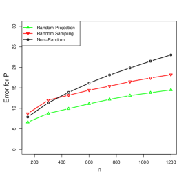
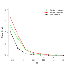
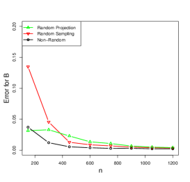
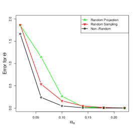
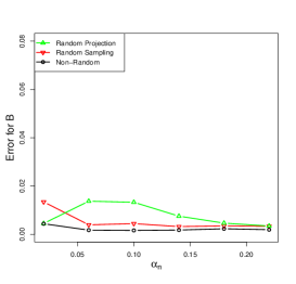
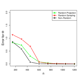
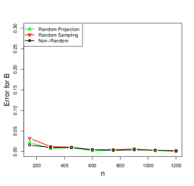
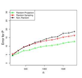
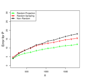
In this experiment, we aim to evaluate the effect of $n$ on the three metrics. To that end, we let $n$ vary while keeping the other parameters fixed at $K=3,\alpha_{n}=0.2,\alpha_{n}(1-\lambda)=0.1,q=2,r=10,p=0.7$. The random test matrix in the random projection scheme was generated with i.i.d. standard Gaussian entries, respectively. Figure 1 shows the average results of 20 replications, where “non-random” refers to the original spectral clustering. Recall that the error bound for $P$ increases with order $O(\sqrt{n})$, the error bound for $\Theta$ decreases with order $O(1/n)$, and the error bound for $B$ vanishes as $n$ goes to infinity. As expected, from Figure 1 we can see that the randomized methods perform worse than the original spectral clustering when $n$ is small, say $n<600$, but they become almost identical when $n$ becomes large, say $n>800$, which is actually the focus of this paper (see Figure 1(b) and (c)). As for the approximation error, we see that the random projection and the random sampling perform better than the original spectral clustering (see Figure 1(a)), which is partially because of the constants’ effects.

Experiment 2.

In this experiment, we evaluate the effect of $\alpha_{n}$ on the three metrics. We fix the sample size for the moment, and focus on the influence of the maximum link probability $\alpha$. Specifically, we let $\alpha$ vary and the between cluster probability was set as $\alpha(1-0.5)$ varying with $\alpha$. The sample size $n$ was fixed at 1152. The other parameters were the same as those in Experiment 1. Figure 2 displays the average results of 20 replications. By the theoretical results, we know that the error bound for $P$ increases with order $O(\sqrt{\alpha})$, the error bound for $\Theta$ decreases with order $O(1/\alpha_{n})$, and the error bound for $B$ decreases ultimately after some increase at the beginning as $\alpha$ increases. The empirical results in Figure 2 coincide with the theoretical results in some sense. The error for $P$ increases slowly with $alpha_{n}$, while the error for $\Theta$ and $B$ both decrease eventually with $\alpha_{n}$. In addition, the gap between the randomized and the original spectral clustering in Figure 2(b) and (c) closes as $\alpha$ increases.

Experiment 3.

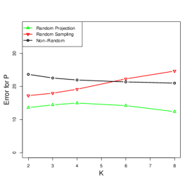
In this experiment, we test the effect of $K$ on the three metrics. Specifically, we let $K$ vary, the within cluster probability $\alpha=0.2$, and the between cluster probability $\alpha(1-0.5)=0.1$, respectively. The other parameters were the same as those in Experiment 2. The average results of 20 replications are shown in Figure 3. The theoretical bounds indicate that the error bound for $\Theta$ increases with order $O(K^{3})$, and the error bound for $B$ increases with $K$. As expected, the empirical results support the theoretical findings (see Figure 3(b) and (c)). The error for $\Theta$ and $B$ both increases with $K$. While for the approximation error, recall that our randomized $\tilde{A}$ attains the minimax optimal rate which does not rely on $K$ (see Theorem 3.6 of Gao et al. (2015)). Empirically, from Figure 3(a) we see that the approximation error for $P$ changes slowly as $K$ increases, which is partially due to the randomness throughout the experimental procedure.

Experiment 4.

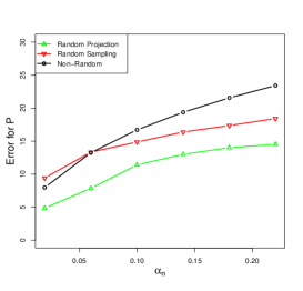
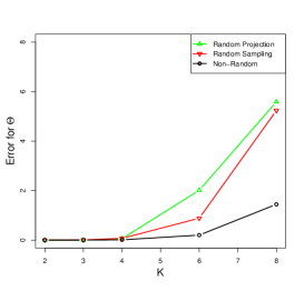
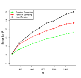
In the above three experiments, we fixed all the other parameters except the one that we pay attention to. Indeed, in view of the theoretical bounds, all the parameters can vary with $n$. To see the so-called high-dimensional performance of each method, in this experiment, we consider a simple setting that the within cluster and between cluster probabilities decrease with $n$ according to $\alpha_{n}=2/\sqrt{n}$ and $\alpha_{n}(1-0.5)=1/\sqrt{n}$, respectively. In such a setting, to ensure the decreasing trend of the misclustered error, $K$ should be of smaller order than $n^{1/6}$, which is rather small for $n$ smaller than, say, 1000. Hence we set $K=2$ for simplicity. The other parameters were the same as those in Experiment 2. Figure 4 shows the average curves for each method in terms of three metrics. As expected, the misclassification error and the error for $B$ both decrease as $n$ increases, showing the high-dimensional feature of the theoretics. In addition, the performance of randomized methods become close to that of the original spectral clustering as $n$ increases.

Figure 1: The average effect of $n$ on the three metrics over 20 replications. (a), (b), (c) correspond to the approximation error for $P$, the misclassification error for $\Theta$, and the estimation error for $B$, respectively. The other parameters $K=3,\alpha_{n}=0.2,\alpha_{n}(1-\lambda)=0.1$, $r=10$, $q=2$, $p=0.7$, and $\Omega$ had i.i.d. standard Gaussian entries, respectively.

Figure 2: The average effect of $\alpha$ on the three metrics over 20 replications. (a), (b), (c) correspond to the approximation error for $P$, the misclassification error for $\Theta$, and the estimation error for $B$, respectively. The other parameters $n=1152,K=3,\lambda=0.5$, $r=10$, $q=2$, $p=0.7$, and $\Omega$ had i.i.d. standard Gaussian entries, respectively.

Figure 3: The average effect of $K$ on the three metrics over 20 replications. (a), (b), (c) correspond to the approximation error for $P$, the misclassification error for $\Theta$, and the estimation error for $B$, respectively. The other parameters $n=1152,\alpha_{n}=0.2,\alpha_{n}(1-\lambda)=0.1$, $r=10$, $q=2$, $p=0.7$, and $\Omega$ had i.i.d. standard Gaussian entries, respectively.

Figure 4: The average effect of $n$ and $\alpha_{n}$ on the three metrics over 20 replications. (a), (b), (c) correspond to the approximation error for $P$, the misclassification error for $\Theta$, and the estimation error for $B$, respectively. The within cluster probability $\alpha_{n}=2/\sqrt{n}$ and the between cluster probability $\alpha_{n}(1-0.5)=1/\sqrt{n}$. The other parameters $K=2$, $r=10$, $q=2$, $p=0.7$, and $\Omega$ had i.i.d. standard Gaussian entries, respectively.

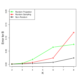
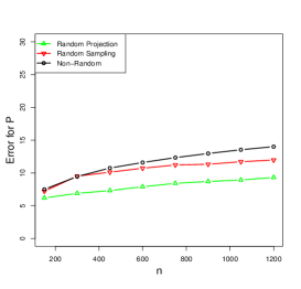
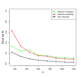
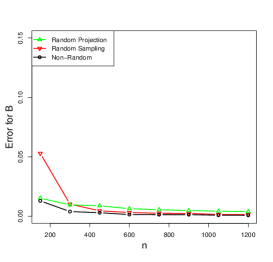
7.2 Model extensions

Besides the simple SBMs we considered in subsection 7.1, we here consider the following six more complex models.

• Model 1 (Full-rank SBM with random $B$): $K=3$, and the elements of $B$ are generated randomly according to $B_{ii}\sim{\rm Uniform}(0.2,0.3)$ and $B_{ij}\sim{\rm Uniform}(0.01,0.1)$, the community sizes are balanced.

• Model 2 (Full-rank SBM with random $B$ and unblanced communities): The parameter set-up is identical to that of Model 1 except that the proportions of the number nodes within of each community over that of the whole nodes are $\frac{1}{6},\frac{1}{2},\frac{1}{3}$, respectively.

• Model 3 (Rank-deficient SBM): $K=3$, and the community sizes are balanced. The link probability matrix $B:=CC^{\intercal}$ where

  $$C:=\left[\begin{matrix}\frac{2{\rm sin}\,0}{3}&\frac{2{\rm cos}\,0}{3}\\ \frac{{\rm sin}\,\frac{\pi}{5}}{2}&\frac{{\rm cos}\,\frac{\pi}{5}}{2}\\ \frac{5{\rm sin}\,\frac{2\pi}{5}}{6}&\frac{5{\rm cos}\,\frac{2\pi}{5}}{6}\end{matrix}\right].$$

• Model 4 (Full-rank DC-SBM): $K=3$, and the elements of $B$ are generated randomly according to $B_{ii}\sim{\rm Uniform}(0.4,0.6)$ and $B_{ij}\sim{\rm Uniform}(0.01,0.2)$. Within each true cluster $k$, $\vartheta_{i\in G_{k}}$’s are i.i.d. 0.2 with probability (w.p.) 0.8, and 1 w.p. 0.2. $\vartheta$’s are then normalized such that its maximum value is 1 within each true cluster.

• Model 5 (Full-rank DC-SBM with more heterogeneity): Except for the node propensity parameter $\vartheta$, the parameter set-up is identical to that of Model 4. The $\vartheta$’s are generated as follows. Within each true cluster $k$, $\vartheta_{i\in G_{k}}$’s are i.i.d. with its element being 0.1 w.p. 0.4, being 0.2 w.p. 0.4, and being 1 with probability 0.2. $\vartheta$’s are then normalized such that its maximum value is 1 within each true cluster.

• Model 6 (Rank-deficient DC-SBM): The parameter set-up is identical to that of Model 4 except the formulation of $B$. Particularly, $B$ is the same with that in Model 3.

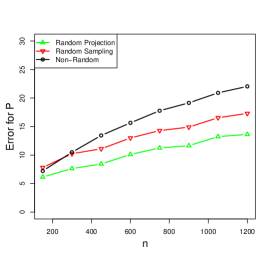
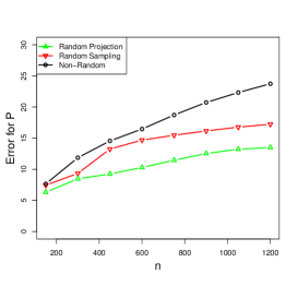
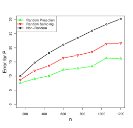
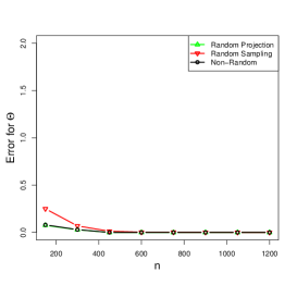
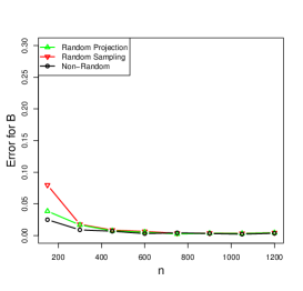
Figure 5 and 6 display the averaged results over 20 replications of model 1-3 and model 4-6, respectively. It can be seen that for all models we tested, the clustering performance of the randomized spectral clustering algorithms become close to that of the original spectral clustering as the sample size $n$ increases, coinciding with theoretical results.

In the above experiments, we only considered assortative networks where nodes tend to be connected with those in the same community, which is mainly because that we require the link probability matrix to be diagonally dominant in some sense (Lemma 2 and 4). For the disassortative networks, it would be our future work to study their clustering methods specifically in the rank deficient setting, though it is suggest that the absolute eigenvalue would help finding the proper communities in full rank setting (Rohe et al., 2011).

(I) Approximation error of model 1, model 2 and model 3.

(II) Misclassification error of Model 1, Model 2 and Model 3.

(III) Estimation error for link probability matrix of model 1, model 2 and model 3.

(a) Model 1

(b) Model 2

(c) Model 3

(d) Model 1

(e) Model 2

(f) Model 3

(g) Model 1

(h) Model 2

(i) Model 3

Figure 5: Averaged results of each method over 20 replications on Models 1-3. Each column corresponds to a model. The first, second and third row corresponds to the approximation error, the misclassification error, and the estimation error for link probability matrix, respectively.

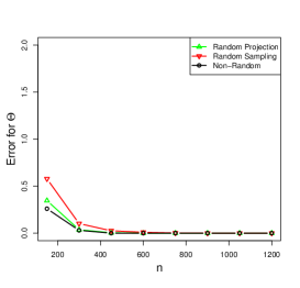
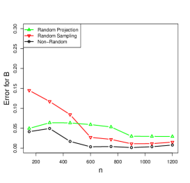
(I) Approximation error of Model 4, Model 5 and Model 6.

(II) Misclassification error of Model 4, Model 5 and Model 6.

(a) Model 4

(b) Model 5

(c) Model 6

(d) Model 4

(e) Model 5

(f) Model 6

Figure 6: Averaged results of each method over 20 replications on Models 4-6. Each column corresponds to a model. The first and second row corresponds to the approximation error and the misclassification error, respectively.

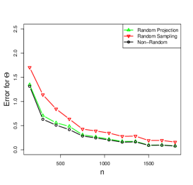
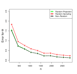
7.3 Additional experiments

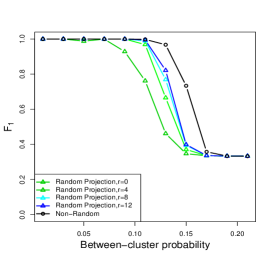
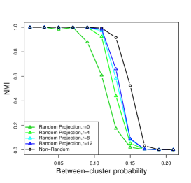
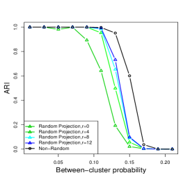
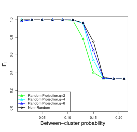
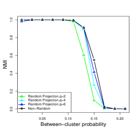
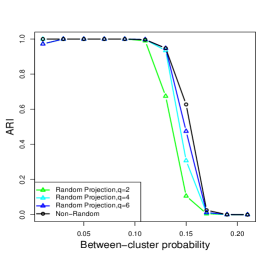
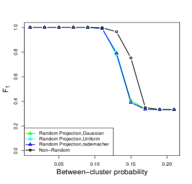
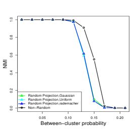
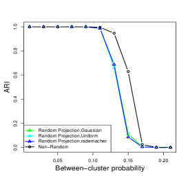
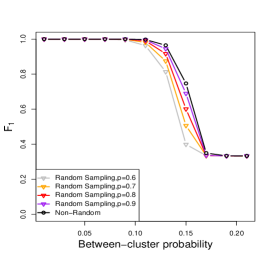
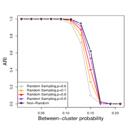
To see how hyper parameters $r,q,p$ and the distribution of test matrix affect the performance of corresponding method, we here conduct another series of experiments. Specifically, to remove the computational cost of finding the best permutation matrix over the permutation matrix set, we use $\rm F_{1}$ score ($\rm F_{1}$), Normalized Mutual Information (NMI), and Adjusted Rand Index (ARI) (Hubert and Arabie, 1985; Manning et al., 2010) to justify the clustering performance of each method. These indexes measure the similarity of two clusters, and here we refer to the estimated and true clusters, from different perspectives. The larger these indexes, the better the clustering algorithm performs. The parameters were basically set as $n=1152$, $K=3$, and the within cluster probability $\alpha=0.2$. To see the effect of other parameters, we varied the oversampling parameter $r\in\{0,4,8,12\}$, the power parameter $q\in\{2,4,6\}$, the sampling rate $p\in\{0.6,0.7,0.8,0.9\}$, and the distribution of test matrix $\Omega$ was generated as i.i.d. Gaussian (standard), uniform (from -1 to 1), and Rademacher (take values $+1$ and $-1$ with equal probability). And for each setting, we let the between cluster probability vary. Figure 7 and 8 show the averaged results of the random projection scheme and the random sampling scheme, respectively. As expected, larger $r$, $q$ and $p$ lead to better clustering performance but at the cost of computational efficiency. One should choose these parameters according to the problem at hand. In addition, among the distribution of $\Omega$ we tested, it has little effect on the resulting clustering performance of random projection.

(I) Effect of the oversampling parameter $r$

(II) Effect of the power parameter $q$

(III) Effect of the test matrix $\Omega$

(a) ${\rm F}_{1}$

(b) NMI

(c) ARI

(d) ${\rm F}_{1}$

(e) NMI

(f) ARI

(g) ${\rm F}_{1}$

(h) NMI

(i) ARI

Figure 7: Effects of the parameters $r,q,\Omega$ in the random projection scheme. Each row corresponds to the effect of one parameter with the others fixed. Each column corresponds to a measure for the clustering performance. The other parameters are fixed at $n=1152$, $K=3$, and the within cluster probability $\alpha=0.2$.

(a) ${\rm F}_{1}$

(b) NMI

(c) ARI

Figure 8: Effect of the parameters $p$ within the random sampling scheme. Each column corresponds to a measure for the clustering performance. The other parameters are fixed at $n=1152$, $K=3$, and the within cluster probability $\alpha=0.2$.

8 Real data examples

In this section, we numerically evaluate the merits of randomized spectral clustering in terms of accuracy and efficiency. Specifically, we first compare the clustering accuracy of each method on four small-scale real networks, using the original spectral clustering as the baseline method. After that, we examine the computational efficiency as well as the relative error of each method on four large-scale networks, where we compare randomized methods with several iterative methods.

8.1 Accuracy evaluation

In this subsection, we test the effectiveness of randomized spectral clustering on four network datasets, including the European email network (Leskovec et al., 2007; Yin et al., 2017), the political blog network (Adamic and Glance, 2005), the statistician coauthor network and the statistician citation network (Ji and Jin, 2016), where the first two datasets have ground truth community assignments and the last two have no ground truth community assignment. Table 1 shows the basic statistics about the networks, where for the first two networks, the target rank is set as the number of true clusters, while for the last two networks, the target rank follows Ji and Jin (2016). For the datasets with ground truth labels, we computed $\rm F_{1}$, NMI, and ARI (Hubert and Arabie, 1985; Manning et al., 2010) between the estimated clusters and the true clusters for each of the three methods, namely, the random projection, the random sampling, and the original spectral clustering, respectively. While for the datasets without ground truth labels, we computed $\rm F_{1}$, NMI, and ARI between the clusters estimated by the randomized spectral clustering and the clusters estimated by the original spectral clustering. Our aim is to show that randomized algorithms perform comparably to the original spectral clustering. Hence for the datasets with ground truth labels, the smaller gap of $\rm F_{1}$, NMI, and ARI between randomized and original spectral clustering indicate the better match between these methods. While for the datasets without ground truth labels, larger $\rm F_{1}$, NMI, and ARI indicate the better match. For the random projection scheme, the oversampling parameter $r=10$, the power parameter $q=2$, and the random test matrix has i.i.d. Gaussian entries. And for the random sampling scheme, we test two cases, namely, $p=0.7$ and $0.8$. Table 2 summarizes the average performance of these methods over 20 replications with the standard deviations in the parentheses. From Table 2 we see that all the methods perform very similarly to each other in terms of $\rm F_{1}$, NMI, and ARI, and the results are rather stable, which shows the effectiveness of randomized methods.

Table 1: A summary of the four small-scale undirected networks.

Networks	No. of nodes	No. of edges	Target rank
European email network	986	16,064	42
Political blog network	1,222	16,714	2
Statisticians coauthor network	2,263	4,388	3
Statisticians citation network	2,654	20,049	3

Table 2: The clustering performance of each method on four real network datasets based on randomized spectral clustering algorithms. For the European email network and political blog network, the performance is evaluated based on a known ground truth. For the statisticians coauthor citation networks, the performance is evaluated based on the original spectral clustering.

Methods	$\rm F_{1}$	NMI	ARI
(a) European email network
Random Projection	0.165(0.007)	0.558(0.006)	0.100(0.009)
Random Sampling ($p=0.7$)	0.126(0.007)	0.417(0.010)	0.059(0.008)
Random Sampling ($p=0.8$)	0.131(0.005)	0.436(0.010)	0.064(0.006)
Non-Random	0.154(0.006)	0.571(0.005)	0.088(0.007)
(b) Political blog network
Random Projection	0.641(0.004)	0.178(0.004)	0.079(0.006)
Random Sampling ($p=0.7$)	0.642(0.003)	0.177(0.007)	0.077(0.007)
Random Sampling ($p=0.8$)	0.641(0.004)	0.177(0.008)	0.077(0.009)
Non-Random	0.641(0.004)	0.178(0.004)	0.079(0.006)
(c) Statisticians coauthor network (No true labels)
Random Projection (relative)	0.981(0.012)	0.646(0.197)	0.715(0.246)
Random Sampling (relative) ($p=0.7$)	0.970(0.011)	0.480(0.148)	0.593(0.193)
Random Sampling (relative) ($p=0.8$)	0.973(0.011)	0.544(0.142)	0.639(0.190)
(d) Statisticians citation network (No true labels)
Random Projection (relative)	0.990(0.021)	0.881(0.166)	0.926(0.140)
Random Sampling (relative) ($p=0.7$)	0.981(0.019)	0.759(0.125)	0.863(0.120)
Random Sampling (relative) ($p=0.8$)	0.981(0.022)	0.770(0.163)	0.861(0.149)

8.2 Efficiency evaluation

In this subsection, we examine the computational efficiency of randomized methods for partial eigenvalue decomposition on four large-scale real undirected networks, including DBLP collaboration network, Youtube social network, Internet topology network, LiveJournal social network (Yang and Leskovec, 2015; Leskovec et al., 2005). These four networks are large-scale with up to millions of nodes and tens of millions of edges. Table 3 shows the basic statistics about the networks, where the target rank corresponds to a network is $k$ if there exits a large gap between the $k$-th and $(k+1)$-th largest (in absolute value) approximated eigenvalues. We compare the performance of our methods with iterative methods, including the implicitly restarted Lanczos algorithm (Calvetti et al., 1994) (svds in R package RSpectra (Qiu and Mei, 2019)), the augmented implicitly restarted Lanczos bidiagonalization algorithms (Baglama and Reichel, 2005) (irlba and partial_eigen in R package irlba (Baglama et al., 2019)). In addition, we also compare our implementation with the randomized methods implemented in svdr in R package irlba (Baglama et al., 2019). Note that the full eigenvalue decomposition always fails in such large-scale data setting.

Table 4 shows the median computational time of each method over 20 replications, where all computations are done on a machine with Intel Core i9-9900K CPU 3.60GHz, 32GB memory, and 64-bit WS operating-system, and R version 4.0.4 is used for all computations. For the random projection-based method, the power parameter is 2 and the oversampling parameter is 10. For the random sampling-based method, the sampling probability is 0.7. We can see from Table 4 that the our methods shows great advantage over compared methods especially when the network scale is large. In particular, the random sampling-based method is efficient no matter the sampling time is included or not.

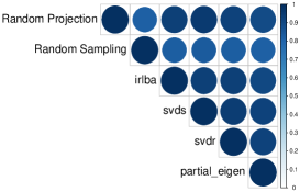
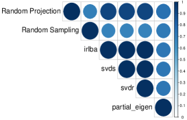
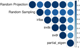
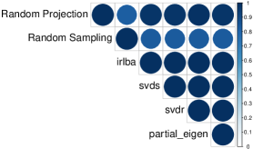
Figure 9 shows the pairwise comparison of the clustering results of six methods on these four networks. The relative clustering performance are measured by ARI. It turns out that the random projection-based method and the random sampling-based method yield similar results with other compared methods, though the random sampling-based method seems to behave slightly different.

Overall, as indicated by our theory and experiments, the randomized methods could bring high efficiency while slightly sacrificing the accuracy. In real world applications, one should balance the accuracy-efficiency trade-off via selecting appropriate hyper parameters according to the real setting.

Table 3: A summary of the four large-scale undirected networks.

Networks	No. of nodes	No. of edges	Target rank
DBLP collaboration network	317,080	1,049,866	3
Youtube social network	1,134,890	2,987,624	7
Internet topology graph	1,696,415	11,095,298	4
LiveJournal social network	3,997,962	34,681,189	4

Table 4: Median time (seconds) of each method for computing the (approximated) eigenvectors of four real network adjacency matrices over 20 replications, where for the random sampling, the time with the sampling time included and excluded (shown in the parentheses) are reported, respectively.

Networks	Random projection	Random sampling	irlba	svds	svdr	partial_eigen
DBLP	0.369	0.280(0.248)	0.341	0.411	6.132	0.346
Youtube	2.037	2.302(2.204)	2.487	3.043	35.595	9.111
Internet	2.773	2.072(1.774)	3.404	3.332	30.900	7.706
LiveJournal	13.213	7.207(6.216)	15.179	20.077	106.166	15.080

(a) DBLP, $K=3$

(b) Youtube, $K=7$

(c) Internet,$K=4$

(d) LiveJournal, $K=4$

Figure 9: The pairwise comparison of the clustering results of six methods on four large-scale networks. The relative clustering performance are measured by ARI. Larger ARI, i.e., larger circles in the figure, indicates that the clustering results of the two methods are more close.

9 Conclusion

In this paper, we used randomized sketching techniques to accelerate the spectral clustering when facing large-scale networks, say networks with millions of nodes, and studied how well the resulting algorithms perform under the SBMs and DC-SBMs. We studied two randomized spectral clustering algorithms. The first one is random projection-based, which reduces the computational cost by projecting the columns and rows of the adjacency matrix to a lower-dimensional space. The second one is random sampling-based, which samples the edges to obtain a sparsified adjacency matrix, and thus reducing the computational cost of partial eigen-decomposition. In the framework of SBMs, we studied these two randomized spectral clustering algorithms in terms of the approximation error that measures the deviation of the randomized adjacency matrix $\tilde{A}$ from the population matrix $P$, the misclassification error that measures the fraction of the number of mis-clustered nodes over the total number of nodes, and the estimation error for the link probability matrix $B$. In particular, we considered a more generalized content where ${\rm rank}(B)$ could be smaller than the cluster number $K$. Under mild conditions, the approximation error turns out to be statistically optimal, which shows that the randomized matrix behaves as if it was sampled from the SBM. We also extend theoretical results to DC-SBMs. Experimental results showed the merits of randomized spectral clustering on networks with up to millions of nodes. For practical convenience, we developed an R package Rclust.

There are many ways that the content in this paper can be extended. First, we studied the weak consistency of the pure spectral clustering without any regularization or refinement, and we mainly used the Davis-Kahan theorem to study the eigenvector perturbation. There exist several works on trimming or refining the pure spectral clustering to help the refined spectral clustering achieve the information-theoretic limit of the exact recovery (strong consistency) or minimax optimal rate of the partial recovery (weak consistency) under SBMs; see Gao et al. (2017); Yun and Proutiere (2016), among others. It would be interesting to study whether one could use similar treatments on the randomized spectral clustering in order to improve its theoretical performance while without increasing the time cost. On the other hand, a few works study the entry-wise perturbation of eigenvectors very recently; see Cape et al. (2019); Tang et al. (2021); Abbe et al. (2020); Su et al. (2019), among others. It would be important and insightful to study the entry-wise perturbation of eigenvectors after randomization, and also study the related strong consistency in SBMs. Second, although the approximation error is minimax optimal under SBMs, it would be important to develop advanced randomization techniques in order to weaken the condition on $\alpha_{n}$, $q$, $p_{ij}$’s. In addition, we mainly focused on the adjacency matrix sampled from the SBMs. It would be interesting to generalize the results to the Laplacian matrix and other network generating models, say–the latent space model, and the graphon models, among others. Finally, it would be important to study the estimation of the model parameters $K$ and ${\rm rank}(B)$ (Fishkind et al., 2013; Ma et al., 2021).

ACKNOWLEDGMENT

We are grateful to the editor, associate editor, and two reviewers for their consideration of our paper and for their helpful suggestions, which led to an improved version of this paper. We also thank Professor Yixuan Qiu for his great help in developing the R package. Our research is partially supported by National Natural Science Foundation of China (No.U1811461), National Natural Science Foundation for Outstanding Young Scholars (No.72122018), and Natural Science Foundation of Shaanxi Province (No. 2021JQ-429 and No.2021JC-01).

Proof of Lemma 1

Denote ${\rm rank}(B)=K^{\prime}$ and define $\Delta={\rm diag}(\sqrt{n_{1}},...,\sqrt{n_{K}})$. It is easy to see that $\Theta\Delta^{-1}$ has orthogonal columns. Write $P$ as

$$P=\Theta B\Theta^{\intercal}=\Theta\Delta^{-1}\Delta B\Delta\Delta^{-1}\Theta^{\intercal}=\Theta\Delta^{-1}LDL^{\intercal}\Delta^{-1}\Theta^{\intercal},$$ (A.1)

where we denote the eigenvalue decomposition of $\Delta B\Delta$ by $L_{K\times K^{\prime}}D_{K^{\prime}\times K^{\prime}}L^{\intercal}_{K^{\prime}\times K}$. Recall that the eigenvalue decomposition of $P$ is $U_{n\times K^{\prime}}\Sigma_{K^{\prime}\times K^{\prime}}U^{\intercal}_{K^{\prime}\times n}$ and note that $\Theta\Delta^{-1}L$ has orthogonal columns, so we obtain ${\Sigma}=D$ and

$${U}=\Theta\Delta^{-1}L.$$ (A.2)

Next we discuss the structure of $U$ respectively when $B$ is of full rank ($K^{\prime}=K$) and rank deficient ($K^{\prime}<K$).

(a) When $K^{\prime}=K$, $\Delta^{-1}L$ is invertible. Thus in this case, $U_{i\ast}=U_{j\ast}$ if and only if $\Theta_{i\ast}=\Theta_{j\ast}$. Moreover, we can verify easily that $\Delta^{-1}L$ has perpendicular rows and the $k$th row has length $\sqrt{1/n_{k}}$, which indicate $\|{U}_{i\ast}-{U}_{j\ast}\|_{2}=\sqrt{(n_{g_{i}})^{-1}+(n_{g_{j}})^{-1}}.$

(b) When $K^{\prime}<K$, $\Delta^{-1}L$ is not invertible. In this case, $\Theta_{i\ast}=\Theta_{j\ast}$ can imply $U_{i\ast}=U_{j\ast}$ by (A.2). On the other hand, by (A.2), we have $\|{U}_{i\ast}-{U}_{j\ast}\|_{2}:=\|\frac{L_{g_{i}\ast}}{\sqrt{n_{g_{i}}}}-\frac{L_{g_{j}\ast}}{\sqrt{n_{g_{j}}}}\|_{2}.$ Hence if the rows of $\Delta^{-1}L$ are mutually distinct with their minimum Euclidean distance being larger than a deterministic sequence $\{\xi_{n}\}_{n\leq 1}$, then $\|{U}_{i\ast}-{U}_{j\ast}\|_{2}\geq\xi_{n}$ for any $\Theta_{i\ast}\neq\Theta_{j\ast}$. $\blacksquare$

Proof of Lemma 2

Suppose $g_{i}=k$ and $g_{j}=l$ ($l\neq k$), and recall that $B=\Delta^{-1}L_{K\times K^{\prime}}D_{K^{\prime}\times K^{\prime}}L^{\intercal}_{K^{\prime}\times K}\Delta^{-1}$, where $D=\Sigma$ and $P=U\Sigma U^{\top}$. Then we have

$$\iota_{n}\|{U}_{i\ast}-{U}_{j\ast}\|_{2}^{2} =\sum_{k_{1}=1}^{K^{\prime}}\iota_{n}(\frac{L_{kk_{1}}}{\sqrt{n_{k}}}-\frac{L_{lk_{1}}}{\sqrt{n_{l}}})^{2}$$

$$\geq\sum_{k_{1}=1}^{K^{\prime}}D_{k_{1}k_{1}}(\frac{L_{kk_{1}}}{\sqrt{n_{k}}}-\frac{L_{lk_{1}}}{\sqrt{n_{l}}})^{2}$$

$$=\sum_{k_{1}=1}^{K^{\prime}}D_{k_{1}k_{1}}(\frac{L_{kk_{1}}}{\sqrt{n_{k}}})^{2}+\sum_{k_{1}=1}^{K^{\prime}}D_{k_{1}k_{1}}(\frac{L_{lk_{1}}}{\sqrt{n_{l}}})^{2}-2\sum_{k_{1}=1}^{K^{\prime}}D_{k_{1}k_{1}}\frac{L_{kk_{1}}L_{lk_{1}}}{\sqrt{n_{k}n_{l}}}$$

$$=B_{kk}+B_{ll}-2B_{kl}$$

$$\geq\eta_{n},$$ (A.3)

where the first and last inequalities are implied by our condition. As a result, for $\Theta_{i\ast}\neq\Theta_{j\ast}$, we obtain $\|{U}_{i\ast}-{U}_{j\ast}\|_{2}\geq\sqrt{\frac{\eta_{n}}{\iota_{n}}}$. $\blacksquare$

Proof of Theorem 1

We use the concentration bound of the non-randomized $A$ around $P$ (Lei and Rinaldo (2015); Chin et al. (2015); Gao et al. (2017)) and the argument about the low-rank randomized approximation in Halko et al. (2011) to bound the derivation of $\tilde{A}^{\rm rp}$ from $P$. We begin by noting that

$$\|\tilde{A}^{\rm rp}-P\|_{2} =\|QQ^{\intercal}AQQ^{\intercal}-P\|_{2}$$

$$\leq\|A-P\|_{2}+\|QQ^{\intercal}AQQ^{\intercal}-A\|_{2}$$

$$=:\mathcal{I}_{1}+\mathcal{I}_{2}.$$ (A.4)

For $\mathcal{I}_{1}$, Lei and Rinaldo (2015) use the delicate combinatorial argument to provide a sharp bound. That is, assume

$${\rm max}_{kl}B_{kl}\leq\alpha_{n}\;{\rm for\;some}\;\alpha_{n}\geq c_{0}\,{\rm log}n/n,$$

then for any $s>0$, there exists a constant $c$ such that

$$\|A-P\|_{2}\leq c\sqrt{n\alpha_{n}}.$$ (A.5)

with probability at least $1-n^{-s}$.

For $\mathcal{I}_{2}$, we first note that

$$\|A-QQ^{\intercal}AQQ^{\intercal}\|_{2} =\|A-QQ^{\intercal}A+QQ^{\intercal}A-QQ^{\intercal}AQQ^{\intercal}\|_{2}$$

$$\leq\|A-QQ^{\intercal}A\|_{2}+\|QQ^{\intercal}(A-AQQ^{\intercal})\|_{2}$$

$$\leq 2\|A-QQ^{\intercal}A\|_{2}.$$ (A.6)

By the Corollary 10.9 and Theorem 9.2 of Halko et al. (2011), when $r\geq 4$, $r{\rm logr}\leq n$ and $q\geq 1$, the following inequality holds with probability at least $1-6\cdot r^{-r}$,

$$\|A-QQ^{\intercal}A\|_{2}\leq\sigma_{K^{\prime}+1}(A)(1+11\sqrt{K^{\prime}+r}\cdot\sqrt{n})^{\frac{1}{2q+1}},$$ (A.7)

where $\sigma_{K^{\prime}+1}(\cdot)$ denotes the $K^{\prime}+1$th largest eigenvalue of a symmetric matrix. Now we bound $\sigma_{K^{\prime}+1}(A)$. Recall that $P=\Theta B\Theta^{\intercal}$ is of rank $K^{\prime}$, then we have

$$\sigma_{K^{\prime}+1}(A)=\sigma_{K^{\prime}+1}(A)-\sigma_{K^{\prime}+1}(P)\leq\|A-P\|_{2}.$$ (A.8)

As a result, with probability at least $1-6\cdot r^{-r}-n^{-s}$

$$\|A-QQ^{\intercal}A\|_{2}\leq c^{\prime}\sqrt{n\alpha_{n}}(1+11\sqrt{K^{\prime}+r}\cdot\sqrt{n})^{\frac{1}{2q+1}}\leq c^{\prime\prime}\sqrt{n\alpha_{n}}(\sqrt{K^{\prime}+r}\cdot\sqrt{n})^{\frac{1}{2q+1}}.$$ (A.9)

When $q=cn^{1/\tau}$ for any $\tau>0$, we can easily prove that $(\sqrt{K^{\prime}+r}\cdot\sqrt{n})^{\frac{1}{2q+1}}=O(1)$ when $n$ goes to infinity. Therefore, we have

$$\mathcal{I}_{2}\leq c\sqrt{n\alpha_{n}}.$$ (A.10)

Finally, combining (A.10) with (A.5), we arrive the results of Theorem 1. $\blacksquare$

Proof of Theorem 2

We make use of the framework in Lei and Rinaldo (2015) to bound the misclustered rate. To fix ideas, we recall some notation now. $U$ and ${U}^{\rm rp}$ denote the $K^{\prime}$ leading eigenvectors of $P=\Theta B\Theta^{\intercal}$ and $\tilde{A}^{\rm rp}$ (the output of Algorithm 2), respectively. ${\tilde{U}}^{\rm rp}:={\tilde{\Theta}}^{\rm rp}{\tilde{X}}^{\rm rp}$ denotes output of the randomized spectral clustering (Algorithm 2). Recall that the heuristic of spectral clustering under the SBM lies in that two nodes are in the same community if and only if their corresponding rows of $U$ are the same (Lei and Rinaldo (2015); Rohe et al. (2011)). Based on these facts, in what follows, we first bound the derivation of ${\tilde{U}}^{\rm rp}$ from $U$. Then, for those nodes within each true cluster that correspond to a large derivation of ${\tilde{U}}^{\rm rp}$ from $U$, we bound their size. At last, we show that for the remaining nodes, the estimated and true clusters coincide.

First, we bound the derivation of $\tilde{U}^{\rm rp}$ from $U$. Davis-Kahan $\rm sin\Theta$ theorem (Theorem VII.3.1 of Bhatia (1997)) provides a useful tool for bounding the perturbation of eigenvectors from the perturbation of matrices. Specifically, by Proposition 2.2 of Vu and Lei (2013), there exists a $K^{\prime}\times K^{\prime}$ orthogonal matrix $O$ such that,

$$\|{U}^{\rm rp}-UO\|_{\tiny\rm F}\leq\frac{2\sqrt{2K^{\prime}}}{\gamma_{n}}\|\tilde{A}^{\rm rp}-P\|_{2}.$$ (A.11)

Now we proceed to derive the Frobenius error of ${\tilde{U}}^{\rm rp}$. Note that

$$\|{\tilde{U}}^{\rm rp}-UO\|_{\tiny\rm F}^{2} =\|{\tilde{U}}^{\rm rp}-{U}^{\rm rp}+{U}^{\rm rp}-UO\|_{\tiny\rm F}^{2}$$

$$\leq\|UO-{U}^{\rm rp}\|_{\tiny\rm F}^{2}+\|{U}^{\rm rp}-UO\|_{\tiny\rm F}^{2}$$

$$=2\|{U}^{\rm rp}-UO\|_{\tiny\rm F}^{2},$$ (A.12)

where the first inequality follows from our assumption that ${\tilde{U}}^{\rm rp}$ is the global solution minimum of the following $k$-means objective and $UO$ is a feasible solution,

$$({\tilde{\Theta}}^{\rm rp},{\tilde{X}}^{\rm rp})=\underset{{\Theta\in\mathbb{M}_{n,K},X\in\mathbb{R}^{K\times K^{\prime}}}}{{\rm arg\;min}}\;\|\Theta X-{U}^{\rm rp}\|_{\rm\tiny F}^{2}.$$

Then combine (Proof of Theorem 2) with (A.11) and the bound of $\|\tilde{A}^{\rm rp}-P\|_{2}$ in Theorem 1, we have with probability larger than $1-6r^{-r}-n^{-s}$ that

$$\|{\tilde{U}}^{\rm rp}-UO\|_{\tiny\rm F}^{2}\leq\frac{cK^{\prime}{n\alpha_{n}}}{\gamma_{n}^{2}}.$$ (A.13)

For notational convenience, we denote the right hand side of (A.13) as ${\rm err}(K^{\prime},n,\alpha_{n},\gamma_{n})$ in what follows.

Then, we proceed to bound the fraction of misclustered nodes. Define

$$S_{k}=\{i\in G_{k}(\Theta):\;\|({\tilde{U}})_{i\ast}^{\rm rp}-(UO)_{i\ast}\|_{\tiny\rm F}>\frac{\delta_{n}}{2}\},$$ (A.14)

where $\delta_{n}$ is defined in Theorem 2 and $S_{k}$ is essentially the number of misclustered nodes in the true cluster $k$ (after some permutation) as we will see soon. By the definition of $S_{k}$, it is easy to see

$$\sum_{k=1}^{K}|S_{k}|\delta_{n}^{2}/4\leq\|{\tilde{U}}^{\rm rp}-UO\|_{\tiny\rm F}^{2}={\rm err}(K^{\prime},n,\alpha_{n},\gamma_{n}).$$ (A.15)

Hence,

$$\sum_{k=1}^{K}\frac{|S_{k}|}{n_{k}}\leq c\frac{{\rm err}(K^{\prime},n,\alpha_{n},\gamma_{n})}{\delta_{n}^{2}{\rm min}\,n_{k}}.$$ (A.16)

Next, we show that the nodes outside $S_{k}$ are correctly clustered. Before that, we first prove $|S_{k}|<n_{k}$. We have by (A.16) that

$$\frac{|S_{k}|}{n_{k}}\leq c\frac{{\rm err}(K^{\prime},n,\alpha_{n},\gamma_{n})}{\delta_{n}^{2}{\rm min}\,n_{k}}.$$ (A.17)

Thus it suffices to prove

$$c\frac{{\rm err}(K^{\prime},n,\alpha_{n},\gamma_{n})}{\delta_{n}^{2}{\rm min}\,n_{k}}<1.$$ (A.18)

which actually follows from the assumption (A4). As a result, we have $|S_{k}|<n_{k}$ for every $1\leq k\leq K$. Therefore, $T_{k}\equiv G_{k}\backslash S_{k}\neq\emptyset$, where we recall that $G_{k}$ denotes the nodes in the true cluster $k$. Let $T=\cup_{k=1}^{K}T_{k}$, we now show that the rows in $(UO)_{T\ast}$ has a one to one correspondence with those in ${\tilde{U}}_{T\ast}^{\rm rp}$. On the one hand, for $i\in T_{k}$ and $j\in T_{l}$ with $l\neq k$, ${\tilde{U}}_{i\ast}^{\rm rp}\neq{\tilde{U}}_{j\ast}^{\rm rp}$, otherwise we have the following contradiction

$$\delta_{n} \leq\|(UO)_{i\ast}-(UO)_{j\ast}\|_{2}$$

$$\leq\|(UO)_{i\ast}-{\tilde{U}}_{i\ast}^{\rm rp}\|_{2}+\|(UO)_{j\ast}-{\tilde{U}}_{j\ast}^{\rm rp}\|_{2}$$

$$<\frac{\delta_{n}}{2}+\frac{\delta_{n}}{2},$$ (A.19)

where the first inequality follows from Lemma 1. On the other hand, for $i,j\in T_{k}$, ${\tilde{U}}_{i\ast}^{\rm rp}={\tilde{U}}_{j\ast}^{\rm rp}$, because otherwise $\tilde{U}_{T\ast}$ has more than $K$ distinct rows which contradicts the fact that the output cluster size is $K$.

Till now, we have proved the membership is correctly recovered outside of $\cup_{k=1}^{K}S_{k}$ and the rate of misclustered nodes in $S_{k}$ is bounded as in (A.16). Therefore we obtain the claim of Theorem 2. $\blacksquare$

Proof of Theorem 3

We first bound the the derivation of ${\tilde{B}}_{ql}^{\rm rp}$ from $B_{ql}$ for each pair of $1\leq q,l\leq K$, then we use the union bound to obtain a bound of $\|{\tilde{B}}^{\rm rp}-B\|_{\infty}$. Denote $\mathcal{E}$ be the event that (4.5) and (4.6) in Theorem 2 hold, which holds with probability larger than $1-6r^{-r}-n^{-s}$ for any $s>0$. In what follows, we derive the bound under the event $\mathcal{E}$.

Note that for any $1\leq q,l\leq K$,

$${B}_{ql}=\frac{\sum_{1\leq i,j\leq n}P_{ij}\Theta_{iq}\Theta_{jl}}{\sum_{1\leq i,j\leq n}\Theta_{iq}\Theta_{jl}}.$$ (A.20)

Then we have the following observations,

$$|{\tilde{B}}_{ql}^{\rm rp}-B_{ql}|$$

$$= \Big{|}\frac{\sum_{1\leq i,j\leq n}\tilde{A}^{\rm rp}_{ij}{\tilde{\Theta}}^{\rm rp}_{iq}{\tilde{\Theta}}^{\rm rp}_{jl}}{\sum_{1\leq i,j\leq n}{\tilde{\Theta}}^{\rm rp}_{iq}{\tilde{\Theta}}^{\rm rp}_{jl}}-\frac{\sum_{1\leq i,j\leq n}P_{ij}\Theta_{iq}\Theta_{jl}}{\sum_{1\leq i,j\leq n}\Theta_{iq}\Theta_{jl}}\Big{|}$$

$$\leq \Big{|}\frac{\sum_{1\leq i,j\leq n}\tilde{A}^{\rm rp}_{ij}{\tilde{\Theta}}^{\rm rp}_{iq}{\tilde{\Theta}}^{\rm rp}_{jl}}{\sum_{1\leq i,j\leq n}{\tilde{\Theta}}^{\rm rp}_{iq}{\tilde{\Theta}}^{\rm rp}_{jl}}-\frac{\sum_{1\leq i,j\leq n}\tilde{A}_{ij}^{\rm rp}\Theta_{iq}\Theta_{jl}}{\sum_{1\leq i,j\leq n}\Theta_{iq}\Theta_{jl}}\Big{|}+\Big{|}\frac{\sum_{1\leq i,j\leq n}\tilde{A}_{ij}^{\rm rp}\Theta_{iq}\Theta_{jl}}{\sum_{1\leq i,j\leq n}\Theta_{iq}\Theta_{jl}}-\frac{\sum_{1\leq i,j\leq n}P_{ij}\Theta_{iq}\Theta_{jl}}{\sum_{1\leq i,j\leq n}\Theta_{iq}\Theta_{jl}}\Big{|}$$

$$=: \mathcal{I}_{1}+\mathcal{I}_{2}.$$ (A.21)

First, for $\mathcal{I}_{2}$, we have

$$\mathcal{I}_{2} \leq\frac{\|\tilde{A}^{\rm rp}-P\|_{\tiny\rm F}(\sum(\Theta_{iq}\Theta_{jl})^{2})^{1/2}}{n_{q}n_{l}}=\frac{\|\tilde{A}^{\rm rp}-P\|_{\tiny\rm F}}{(n_{q}n_{l})^{1/2}}$$

$$\leq\frac{\sqrt{K^{\prime}+r}\|\tilde{A}^{\rm rp}-P\|_{2}}{(n_{q}n_{l})^{1/2}}$$

$$\leq\frac{c\sqrt{K^{\prime}+r}\sqrt{n\alpha_{n}}}{(n_{q}n_{l})^{1/2}}$$ (A.22)

where the first inequality follows from the Cauchy-Schwarz’s inequality and the fact that $\sum_{1\leq i,j\leq n}\Theta_{iq}\Theta_{jl}=n_{q}n_{l}$, the second inequality follows from $\|A\|_{\rm F}\leq\sqrt{{\rm rank}(A)}\|A\|_{2}$ for any matrix $A$ and the fact that $\tilde{A}^{\rm rp}-P$ has rank at most $K^{\prime}+r$, and the last inequality is implied by the spectral bound of $\tilde{A}^{\rm rp}-P$ (see (4.1)).

Next, we bound $\mathcal{I}_{1}$. We have

$$\mathcal{I}_{1}\leq \Big{|}\frac{\sum_{1\leq i,j\leq n}\tilde{A}^{\rm rp}_{ij}{\tilde{\Theta}}^{\rm rp}_{iq}{\tilde{\Theta}}^{\rm rp}_{jl}}{\sum_{1\leq i,j\leq n}{\tilde{\Theta}}^{\rm rp}_{iq}{\tilde{\Theta}}^{\rm rp}_{jl}}-\frac{\sum_{1\leq i,j\leq n}\tilde{A}^{\rm rp}_{ij}{{\Theta}}^{\rm rp}_{iq}{{\Theta}}^{\rm rp}_{jl}}{\sum_{1\leq i,j\leq n}{\tilde{\Theta}}^{\rm rp}_{iq}{\tilde{\Theta}}^{\rm rp}_{jl}}\Big{|}+\Big{|}\frac{\sum_{1\leq i,j\leq n}\tilde{A}^{\rm rp}_{ij}{{\Theta}}^{\rm rp}_{iq}{{\Theta}}^{\rm rp}_{jl}}{\sum_{1\leq i,j\leq n}{\tilde{\Theta}}^{\rm rp}_{iq}{\tilde{\Theta}}^{\rm rp}_{jl}}-\frac{\sum_{1\leq i,j\leq n}\tilde{A}^{\rm rp}_{ij}{{\Theta}}^{\rm rp}_{iq}{{\Theta}}^{\rm rp}_{jl}}{\sum_{1\leq i,j\leq n}{{\Theta}}^{\rm rp}_{iq}{{\Theta}}^{\rm rp}_{jl}}\Big{|}$$

$$=: \mathcal{I}_{11}+\mathcal{I}_{12}.$$ (A.23)

For $1\leq q\leq K$, denote the $\hat{n}_{q}$ be the number of nodes in the $q$th estimated cluster, that is, $\sum_{i}\tilde{{\Theta}}^{\rm rp}_{iq}=\hat{n}_{q}$. Then we have for $\mathcal{I}_{11}$ that,

$$\mathcal{I}_{11} \leq\frac{1}{\hat{n}_{q}\hat{n}_{l}}\|\tilde{A}^{\rm rp}\|_{\rm F}(\sum_{i,j}({\Theta}^{\rm rp}_{iq}{{\Theta}}^{\rm rp}_{jl}+{\tilde{\Theta}}^{\rm rp}_{iq}{\tilde{\Theta}}^{\rm rp}_{jl})^{2})^{1/2}$$

$$\leq\frac{1}{\hat{n}_{q}\hat{n}_{l}}\|\tilde{A}^{\rm rp}\|_{\rm F}((n_{q}n_{l})^{1/2}+(\hat{n}_{q}\hat{n}_{l})^{1/2})$$

$$=\|\tilde{A}^{\rm rp}\|_{\rm F}(\frac{1}{(\hat{n}_{q}\hat{n}_{l})^{1/2}}+\frac{({n}_{q}{n}_{l})^{1/2}}{\hat{n}_{q}\hat{n}_{l}}),$$ (A.24)

where the first and second inequality follows from the Cauchy-Schwarz’s inequality and the triangle inequality, respectively. Using the Cauchy-Schwarz’s inequality again, we have for $\mathcal{I}_{12}$ that,

$$\mathcal{I}_{12}\leq|\sum_{ij}\tilde{A}^{\rm rp}_{ij}{\Theta}^{\rm rp}_{iq}{{\Theta}}^{\rm rp}_{jl}||\frac{1}{n_{q}n_{l}}-\frac{1}{\hat{n}_{q}\hat{n}_{l}}|\leq\|\tilde{A}^{\rm rp}\|_{\rm F}(\frac{1}{({n}_{q}{n}_{l})^{1/2}}+\frac{({n}_{q}{n}_{l})^{1/2}}{\hat{n}_{q}\hat{n}_{l}}).$$ (A.25)

Putting (A.25) and (Proof of Theorem 3) together, we have for $\mathcal{I}_{1}$ that,

$$\mathcal{I}_{1} \leq\|\tilde{A}^{\rm rp}\|_{\rm\tiny F}(\frac{1}{({n}_{q}{n}_{l})^{1/2}}+\frac{1}{(\hat{n}_{q}\hat{n}_{l})^{1/2}}+2\frac{({n}_{q}{n}_{l})^{1/2}}{\hat{n}_{q}\hat{n}_{l}})$$

$$\leq(\|\tilde{A}^{\rm rp}-P\|_{\rm\tiny F}+\|P\|_{\rm\tiny F})(\frac{1}{({n}_{q}{n}_{l})^{1/2}}+\frac{1}{(\hat{n}_{q}\hat{n}_{l})^{1/2}}+2\frac{({n}_{q}{n}_{l})^{1/2}}{\hat{n}_{q}\hat{n}_{l}})$$

$$\leq(c\sqrt{K^{\prime}+r}\sqrt{n\alpha_{n}}+\sqrt{K^{\prime}}\sigma_{n})(\frac{1}{({n}_{q}{n}_{l})^{1/2}}+\frac{1}{(\hat{n}_{q}\hat{n}_{l})^{1/2}}+2\frac{({n}_{q}{n}_{l})^{1/2}}{\hat{n}_{q}\hat{n}_{l}}),$$ (A.26)

where the last inequality is implied by $\|A\|_{\rm F}\leq\sqrt{{\rm rank}(A)}\|A\|_{2}$ for any matrix $A$ and the following facts, $\tilde{A}^{\rm rp}-P$ has rank at most $K^{\prime}+r$, $P$ has rank $K^{\prime}$, the spectral bound of $\tilde{A}^{\rm rp}-P$ (see (4.1)), and the largest eigenvalue of $P$ is $\sigma_{n}$. To further bound (Proof of Theorem 3), we now discuss the relationship between $n_{k}$ and $\hat{n}_{k}$. Recall (4.6), we see that $S_{k}$ is the number of misclustered nodes in the $k$th true cluster. Hence we have

$$\hat{n}_{k}\geq n_{k}-S_{k}\geq n_{k}-n_{k}c_{3}^{-1}\frac{K^{\prime}n\alpha_{n}}{\gamma_{n}^{2}}=n_{k}(1-c_{3}^{-1}\frac{K^{\prime}n\alpha_{n}}{\gamma_{n}^{2}\delta_{n}^{2}{\rm min}\,n_{k}}),$$ (A.27)

where the second inequality follows from (4.6), namely, the error bound for the sum of misclassification error over all $K$ clusters. Combining (A.27) with (Proof of Theorem 3), we have the bound for $\mathcal{I}_{1}$,

$$\mathcal{I}_{1} \leq c(\frac{\sqrt{K^{\prime}+r}\sqrt{n\alpha_{n}}}{{\rm min}\,n_{k}}+\frac{\sqrt{K^{\prime}}\sigma_{n}}{{\rm min}\,n_{k}})\left(1+(1-\Phi_{n})^{-1}+\frac{2{\rm max}\,n_{k}}{{\rm min}\,n_{k}}(1-\Phi_{n})^{-2}\right),$$ (A.28)

where $\Phi_{n}:=c_{3}^{-1}\frac{K^{\prime}n\alpha_{n}}{\gamma_{n}^{2}\delta_{n}^{2}{\rm min}\,n_{k}}$ Consequently, combining (A.28) with (Proof of Theorem 3), we obtain the bound for $|{\tilde{B}}_{ql}^{\rm rp}-B_{ql}|$. Finally, considering the event $\mathcal{E}$ and using the union bound, we obtain the desired bound for $\|{\tilde{B}}^{\rm rp}-B\|_{\infty}$. $\blacksquare$

Proof of Theorem 4

Before deriving the spectral error bound of $\tilde{A}^{\rm rs}$ from $P$, we first give some notation. Recall that $\tilde{A}^{\rm rs}$ is obtained by two steps: (a) Randomly select pair $(i,j)$ of the adjacency matrix $A$ independently with probability $p_{ij}$ regardless of the value of $A_{ij}$, and for each pair $(i,j)(i<j)$, the symmetric sparsified matrix $\tilde{A}^{\rm s}$ is defined as $\tilde{A}_{ij}^{\rm s}=\frac{A_{ij}}{p_{ij}}$ if $(i,j)$ is selected, and $\tilde{A}_{ij}^{\rm s}=0$ otherwise, (b) Apply an iterative algorithm to find the nearly-optimal rank $K^{\prime}$ approximation $\tilde{A}^{\rm rs}$ of $A^{\rm s}$. Let ${G}$ be the adjacency matrix of an Erodös-Renyi graph with edge $(i,j)$ being with probability $0<p_{ij}<1$. Define $\bar{P}=\left(\frac{1}{p_{ij}}\right)\in\mathbb{R}^{n^{2}}$. Then it is obvious that $\tilde{A}_{s}$ in (a) can be written as ${\tilde{A}_{s}=\bar{P}\circ G\circ A}$, where $\circ$ denotes the element-wise multiplication. To simplify the proof, we assume that (b) finds the exactly optimal rank $K^{\prime}$ approximation $\tilde{A}^{\rm rs}$ of $\tilde{A}^{\rm s}$, i.e.,

$$\tilde{A}^{\rm rs}={\rm arg\,min}\;_{{\rm rank}(M)\leq K^{\prime}}\|\tilde{A}_{s}-M\|_{2}={\rm arg\,min}\;_{{\rm rank}(M)\leq K^{\prime}}\|\bar{P}\circ G\circ A-M\|_{2}.$$ (A.29)

Now we proceed to derive the error bound of $\tilde{A}^{\rm rs}$ from $P$. Note that

$$\|\tilde{A}^{\rm rs}-P\|_{2} \leq\|\tilde{A}^{\rm rs}-\bar{P}\circ G\circ A\|_{2}+\|\bar{P}\circ G\circ A-P\|_{2}$$

$$\leq 2\|\bar{P}\circ G\circ A-P\|_{2}=2\|\bar{P}\circ G\circ(A-P)+\bar{P}\circ G\circ P-P\|_{2}$$

$$\leq 2\|\bar{P}\circ G\circ(A-P)\|_{2}+2\|\bar{P}\circ G\circ P-P\|_{2},$$

$$=\mathcal{I}_{1}+\mathcal{I}_{2},$$ (A.30)

where the second inequality follows from (A.29) and the fact that ${\rm rank}(P)=K^{\prime}$.

To bound $\mathcal{I}_{1}$ and $\mathcal{I}_{2}$, we need the following results on the spectral-norm bound of a random matrix with symmetric independent and bounded entries (see Proposition 1 of Chen and Wainwright (2015); Corollaries 3.6 and 3.12 in Bandeira et al. (2016)).

Proposition 1

Let $X$ be an $n\times n$ symmetric random matrix whose entries $X_{ij}$’s are independent symmetric random variables and bounded such that ${\rm max}_{ij}|X_{ij}|\leq\sigma_{1}$. Define

$$\sigma_{2}={\rm max}_{i}\sqrt{\mathbb{E}\sum_{j}X_{ij}^{2}}.$$ (A.31)

Then there exists universal constants $c$ and $c^{\prime}$ such that,

$$\quad\quad\quad\quad\mathbb{E}\|X\|_{2}\leq 3\sigma_{2}+c\sigma_{1}\sqrt{{\rm log}n},$$

$$\mathbb{P}(\|X\|_{2}\geq 3\sigma_{2}+t)\leq n\cdot{\rm exp}(-\frac{t^{2}}{c^{\prime}\sigma_{1}^{2}})\;{\mbox{ for any}}\;\,t\geq 0.$$ (A.32)

We first bound $\mathcal{I}_{1}=2\|\bar{P}\circ G\circ(A-P)\|_{2}$ by conditioning on $A-P\equiv W$, where $\bar{P}\circ G\circ W$ is the $X$ in Proposition 1. We have $(\bar{P}\circ G\circ W)_{ij}=b_{ij}\frac{W_{ij}}{p_{ij}}$, where $b_{ij}\sim{\rm Bernoulli}(p_{ij})$. It is easy to see that ${\rm max}_{ij}|b_{ij}\frac{W_{ij}}{p_{ij}}|\leq\frac{2}{p_{\rm min}}$, so we can set $\sigma_{1}=\frac{2}{p_{\rm min}}$. And we also have,

$$\sigma_{2} ={\rm max}_{i}\sqrt{\mathbb{E}(\sum_{j}b_{ij}^{2}\frac{W_{ij}^{2}}{p_{ij}^{2}}|W)}={\rm max}_{i}\sqrt{\sum_{j}\frac{W_{ij}^{2}}{p_{ij}^{2}}\mathbb{E}(b_{ij}^{2}|W)}$$

$$\leq{\rm max}_{i}\;p_{\rm min}^{-1/2}\sqrt{\|W_{i\ast}\|_{2}^{2}}=p_{\rm min}^{-1/2}\sqrt{\|W\|_{2,\infty}^{2}}\leq p_{\rm min}^{-1/2}\|W\|_{2},$$ (A.33)

where for any matrix $B$, $\|B\|_{2,\infty}:={\rm max}_{i}(\sum_{j}B_{ij}^{2})^{1/2}$ and the last inequality follows from the fact that $\|W\|_{2,\infty}\leq\|W\|_{2}$. Alternatively, we can obtain $\sigma_{2}\leq c\sqrt{{\rm max}_{i}\sum_{j}\frac{1}{p_{ij}}}$ if we repeat the steps in (Proof of Theorem 4) and take summation over $\mathbb{E}(b_{ij}^{2}|W)/p_{ij}^{2}$. Hence, $\sigma_{2}\leq c{\rm min}\,\{p_{\rm min}^{-1/2}\|W\|_{2},\sqrt{{\rm max}_{i}\sum_{j}\frac{1}{p_{ij}}}\}$. Choosing $t=c\sigma_{1}\sqrt{{\rm log}n}$ in Proposition 1 for large enough constant $c>0$, then there exists constant $\nu_{1}>0$ such that with probability larger than $1-n^{\nu_{1}}$,

$$\mathcal{I}_{1}=2\|\bar{P}\circ G\circ(A-P)\|_{2}\leq c\,{\rm max}\,\Big{\{}{\rm min}\,\big{\{}p_{\rm min}^{-1/2}\|W\|_{2},\sqrt{{\rm max}_{i}\sum_{j}{p_{ij}^{-1}}}\big{\}},\;\frac{\sqrt{{\rm log}n}}{p_{\rm min}}\Big{\}}.$$ (A.34)

To further bound $\mathcal{I}_{1}$, we use the following spectral norm error bound of $A-P$ proved in Lei and Rinaldo (2015). That is, under assumption (A2),

$$\|W\|_{2}=\|A-P\|_{2}\leq c\sqrt{n\alpha_{n}},$$ (A.35)

with probability larger than $1-n^{-\nu_{1}}$, where we set $\nu_{1}$ to be identical to that corresponds to (A.34). As a result, we have with probability larger than $1-2n^{-\nu_{1}}$ that,

$$\mathcal{I}_{1}\leq c\,{\rm max}\,\Big{\{}{\rm min}\,\big{\{}p_{\rm min}^{-1/2}\sqrt{n\alpha_{n}},\sqrt{{\rm max}_{i}\sum_{j}{p_{ij}^{-1}}}\big{\}},\;\frac{\sqrt{{\rm log}n}}{p_{\rm min}}\Big{\}}.$$ (A.36)

Next, we use Proposition 1 again to bound $\mathcal{I}_{2}=2\|\bar{P}\circ G\circ P-P\|_{2}$. We first have

$${\rm max}_{ij}|\frac{1}{p_{ij}}G_{ij}P_{ij}-P_{ij}|\leq{\rm max}\{1,\frac{1}{p_{\rm min}}-1\}\cdot\alpha_{n}.$$ (A.37)

Hence we can set $\sigma_{1}={\rm max}\{1,\frac{1}{p_{\rm min}}-1\}\cdot\alpha_{n}$. For $\sigma_{2}$, we have

$$\sigma_{2} ={\rm max}_{i}\sqrt{\mathbb{E}(\sum_{j}[(\frac{1}{p_{ij}}G_{ij}-1)^{2}P_{ij}^{2})]}={\rm max}_{i}\sqrt{\sum_{j}\alpha_{n}^{2}\mathbb{E}(\frac{1}{p_{ij}}G_{ij}-1)^{2}}\leq\sqrt{\alpha_{n}^{2}{\rm max}_{i}\sum_{j}(\frac{1}{p_{ij}}-1)}.$$ (A.38)

Selecting $t=c\sigma_{1}\sqrt{{\rm log}n}$ in Proposition 1 for large enough constant $c>0$, then there exists constant $\nu_{2}>0$ such that with probability larger than $1-n^{-\nu_{2}}$,

$$\mathcal{I}_{2}\leq c\,{\rm max}\left(\sqrt{\alpha_{n}^{2}{\rm max}_{i}\sum_{j}(\frac{1}{p_{ij}}-1)},\;{\rm max}\{1,\frac{1}{p_{\rm min}}-1\}\cdot\alpha_{n}\sqrt{{\rm log}n}\right).$$ (A.39)

Consequently, combining (A.36) with (A.39), we have with probability larger than $1-c_{6}n^{-\nu}$ that

$$\|\tilde{A}^{\rm rs}-P\|_{2} =\mathcal{I}_{1}+\mathcal{I}_{2}$$

$$\leq c\,{\rm max}\Big{\{}I_{1},\;\frac{\sqrt{{\rm log}n}}{p_{\rm min}},\,\sqrt{n\alpha_{n}^{2}(\frac{1}{p_{\rm min}}-1)},\;\sqrt{\alpha_{n}^{2}{\rm log}n{\rm max}\{1,\frac{1}{p_{\rm min}}-1\}^{2}}\Big{\}},$$ (A.40)

where $\nu={\rm min}\{\nu_{1},\nu_{2}\}$ and $I_{1}:={\rm min}\Big{\{}\sqrt{\frac{n\alpha_{n}}{p_{\rm min}}},\sqrt{{\rm max}_{i}\sum_{j}\frac{1}{p_{ij}}}\Big{\}}$. The conclusion in Theorem 4 is arrived. $\blacksquare$

Proof of Lemma 3

Let $\tilde{\vartheta}$ be an $n\times 1$ vector such that the $i$th element is $\vartheta_{i}/\|\phi_{g_{i}}\|_{2}$, where recall that $\phi_{k}$ is an $n\times 1$ vector that consistent with $\vartheta$ on $G_{k}$ and zero otherwise. Let $\bar{\Theta}$ be the normalized membership matrix such that $\bar{\Theta}(i,k)=\bar{\vartheta}_{i}$ if $i\in G_{k}$ and $\bar{\Theta}(i,k)=0$. And it can be verified that $\bar{\Theta}^{\intercal}\bar{\Theta}=I.$ Recall $\Omega={\rm diag}(\|\phi_{1}\|_{2},...,\|\phi_{K}\|_{2})$. Then we have

$${\rm diag}(\vartheta)\Theta=\bar{\Theta}\Omega.$$ (A.41)

As a result,

$$P={\rm diag}(\vartheta)\Theta B\Theta^{\intercal}{\rm diag}(\vartheta)=\bar{\Theta}\Omega B\Omega\bar{\Theta}^{\intercal}=\bar{\Theta}HDH^{\intercal}\bar{\Theta}^{\intercal},$$ (A.42)

where we denote the eigenvalue decomposition of $\Omega B\Omega$ by

$$\Omega B\Omega=H_{K\times K^{\prime}}D_{K^{\prime}\times K^{\prime}}H_{K^{\prime}\times K}^{\intercal},$$ (A.43)

where $H$ has orthogonal columns. Recall that we also have $P=U\Sigma U^{\intercal}$, hence by the orthonormality of $\bar{\Theta}$ and $H$, we have

$${U}=\bar{\Theta}H,\quad{\Sigma}=D.$$ (A.44)

Specifically, ${U}_{i\ast}=\tilde{\vartheta}_{i}H_{k\ast}$ for $i\in G_{k}$.

Now we discuss the structure of $U$ respectively when $B$ is of full rank ($K^{\prime}=K$) and rank deficient ($K^{\prime}<K$).

(a) When $K^{\prime}=K$, $H$ is a square matrix with orthogonal columns, implying that the rows of $H$ are perpendicular with each other. As a result, ${\rm cos}({U}_{i\ast},{U}_{j\ast})=0$ if $g_{i}\neq g_{j}$ and ${\rm cos}({U}_{i\ast},{U}_{j\ast})=1$ if $g_{i}=g_{j}$.

(b) When $K^{\prime}<K$, it is straightforward that ${\rm cos}({U}_{i\ast},{U}_{j\ast})=1$ if $g_{i}=g_{j}$. For $g_{i}\neq g_{j}$, without loss of generality we assume $g_{i}=k,g_{j}=l(l\neq k)$. In this case, we observe that ${\rm cos}({U}_{i\ast},{U}_{j\ast})={\rm cos}({H}_{k\ast},{H}_{l\ast})$. Therefore, by the condition that $\max_{k,l}{\rm cos}({H}_{k\ast},{H}_{l\ast})<\xi^{\prime}_{n}<1$, we arrive the conclusion of Lemma 3. $\blacksquare$

Proof of Lemma 4

First, we show that for any $1\leq k\leq K$, $\|{H}_{k\ast}\|_{2}\neq 0$, which excludes the trivial case that ${\rm cos}({H}_{k\ast},{H}_{l\ast})=1$ for $k\neq l$. To see this, by (A.43), (A.44) and the condition that for any $1\leq i\leq K^{\prime}$, $0<\Sigma_{ii}<\overline{\iota}_{n}$, we have

$$\overline{\iota}_{n}\|{H}_{k\ast}\|_{2}^{2}\geq\sum_{k_{1}=1}^{K^{\prime}}D_{k_{1}k_{1}}H_{kk_{1}}^{2}=\bar{B}_{kk}>0,$$

where the last inequality follows from the assumption that $B_{kk}>0$ for any $1\leq k\leq K$ and the definition of $\bar{B}$.

Second, we show that for any $\lambda$ and any $1\leq k<l\leq K$, $\|{H}_{k\ast}-\lambda{H}_{l\ast}\|_{2}^{2}>0$ under our condition, which indicates that ${\rm cos}({H}_{k\ast},{H}_{l\ast})<1$. In fact, we can observe that

$$\overline{\iota}_{n}\|{H}_{k\ast}-\lambda{H}_{l\ast}\|_{2}^{2}\geq\sum_{k_{1}=1}^{K^{\prime}}D_{k_{1}k_{1}}(H_{kk_{1}}-\lambda H_{lk_{1}})^{2}=\lambda^{2}\bar{B}_{ll}-2\lambda\bar{B}_{kl}+\bar{B}_{kk}.$$ (A.45)

Note that the RHS of (A.45) is a parabola of form $a\lambda^{2}+b\lambda+c$ with $a:=\bar{B}_{ll}$, $b:=-2\bar{B}_{kl}$, and $c:=\bar{B}_{kk}$. Also note that $\bar{B}_{ll}>0$, hence the RHS of (A.45) is always larger than 0 if the discriminant $b^{2}-4ac:=4\bar{B}_{kl}^{2}-4\bar{B}_{kk}\bar{B}_{ll}<0$, which is actually our condition.

Third, we give an explicit bound for ${\rm cos}({H}_{k\ast},{H}_{l\ast})$. Choosing $\lambda=-\frac{2a}{b}$, we obtain that

$$\lambda^{2}\bar{B}_{ll}-2\lambda\bar{B}_{kl}+\bar{B}_{kk}\geq\frac{-b^{2}+4ac}{4a}:=\frac{-\bar{B}_{kl}^{2}+\bar{B}_{kk}\bar{B}_{ll}}{\bar{B}_{ll}}\geq\frac{\eta^{\prime}_{n}}{\beta_{n}}>0,$$

where the last inequality follows from our conditions. Hence by (A.45), for any $\lambda$, we have

$$\|{H}_{k\ast}-\lambda{H}_{l\ast}\|_{2}^{2}\geq\frac{\eta^{\prime}_{n}}{\overline{\iota}_{n}\beta_{n}}.$$ (A.46)

Note that the LHS of (A.46) is also a parabola. Choosing $\lambda=\frac{{H}_{k\ast}{H}_{l\ast}^{\intercal}}{\|{H}_{l\ast}\|_{2}^{2}}$, we thus have

$$\frac{-({H}_{k\ast}{H}_{l\ast}^{\intercal})^{2}+\|{H}_{l\ast}\|_{2}^{2}\|{H}_{k\ast}\|_{2}^{2}}{\|{H}_{l\ast}\|_{2}^{2}}\geq\frac{\eta^{\prime}_{n}}{\overline{\iota}_{n}\beta_{n}},$$

which implies

$${\rm cos}({H}_{k\ast},{H}_{l\ast})\leq\sqrt{1-\frac{\eta^{\prime}_{n}}{\overline{\iota}_{n}\beta_{n}\|{H}_{k\ast}\|_{2}^{2}}}\leq\sqrt{1-\frac{\eta^{\prime}_{n}}{\overline{\iota}_{n}\beta_{n}^{2}/\underline{\iota}_{n}}},$$

where in the last inequality, we used the fact that

$$\underline{\iota}_{n}\|{H}_{k\ast}\|_{2}^{2}\leq\sum_{k_{1}=1}^{K^{\prime}}D_{k_{1}k_{1}}H_{kk_{1}}^{2}=\bar{B}_{kk}<\beta_{n}.$$

The proof is completed. $\blacksquare$

Proof of Theorem 7

The proof is similar to that of Theorem 2 except that we need to handel the normalized eigenvectors and the eigenvectors with 0 norm. To fix ideas, we recall and introduce some notation now. With slight abuse of notation, $U$ and $\hat{U}$ denote the $K^{\prime}$ leading eigenvectors of $P=\Theta B\Theta^{\intercal}$ and $\tilde{A}$, respectively. ${\tilde{U}}$ denotes the output of the randomized spherical spectral clustering. ${{U}}^{\prime}$ denotes the normalized ${U}$, namely, ${U}^{\prime}_{i\ast}=U_{i\ast}/\|U_{i\ast}\|_{2}$. ${\hat{U}}^{\prime}$ denotes the normalized ${\hat{U}}$, namely, ${\hat{U}}^{\prime}_{i\ast}={\hat{U}}_{i\ast}/\|{\hat{U}}_{i\ast}\|_{2}$ and ${\hat{U}}^{\prime}_{i\ast}:=0$ if $\|{\hat{U}}_{i\ast}\|_{2}=0$.

First, following the same proof strategy with that in Theorem 2, there exists a $K^{\prime}\times K^{\prime}$ orthogonal matrix $O$ such that,

$$\|{\hat{U}}-UO\|_{\tiny\rm F}^{2}\leq\frac{cK^{\prime}{\|A-P\|_{2}^{2}}}{\gamma_{n}^{2}}.$$ (A.47)

For notational simplicity, in what follows we assume the orthogonal matrix $O$ is the identity matrix. Note that $U$’s rows are all non-zero. To see this, recall in (A.43), we have shown that ${U}_{i\ast}=\tilde{\vartheta}_{i}H_{k\ast}$ for $i\in G_{k}$, where $H_{K\times K^{\prime}}$ has orthogonal columns. When $K^{\prime}=K$, $H$ is an orthonormal matrix, hence we have

$$\|U_{i\ast}\|_{2}^{2}=\tilde{\vartheta}_{i}^{2}.$$ (A.48)

When $K^{\prime}<K$, by our condition that $0<\Sigma_{ii}<\overline{\iota}_{n}$ and ${B}_{kk}>0$ we have

$$\overline{\iota}_{n}\|{H}_{k\ast}\|_{2}^{2}\geq\sum_{k_{1}=1}^{K^{\prime}}D_{k_{1}k_{1}}H_{kk_{1}}^{2}=\bar{B}_{kk}>0,$$

which implies that

$$\|U_{i\ast}\|_{2}^{2}=\tilde{\vartheta}_{i}^{2}\|H_{k\ast}\|_{2}^{2}\geq\tilde{\vartheta}_{i}^{2}\bar{B}_{kk}/\overline{\iota}_{n}.$$ (A.49)

For any vectors $a$ and $b$, the fact that

$$\|\frac{a}{\|a\|_{2}}-\frac{b}{\|b\|_{2}}\|_{2}\leq 2\frac{\|a-b\|_{2}}{{\rm max}(\|a\|_{2},\|b\|_{2})}$$

holds, and for any $a=0$, $\|0-\frac{b}{\|b\|_{2}}\|_{2}\leq 2\frac{\|0-b\|_{2}}{\|b\|_{2}}$ holds trivially. We thus have

$$\|{\hat{U}}^{\prime}-U^{\prime}\|_{\tiny\rm F}^{2}\leq c\sum_{i=1}^{n}\frac{\|{\hat{U}}_{i\ast}-{U}_{i\ast}\|_{2}^{2}}{\|{U}_{i\ast}\|_{2}^{2}}\leq\frac{\|{\hat{U}}-U\|_{\tiny\rm F}^{2}}{\min_{i}\|{U}_{i\ast}\|_{2}^{2}}\leq c\frac{K^{\prime}{\|A-P\|_{2}^{2}}}{\gamma_{n}^{2}\min_{i}\|{U}_{i\ast}\|_{2}^{2}},$$ (A.50)

where the last inequality follows from (A.47) and $\min_{i}\|{U}_{i\ast}\|_{2}^{2}$ can be lower bounded differently depending on $K^{\prime}=K$ (see (A.48)) or $K^{\prime}<K$ (see (A.49)). Further, by the fact that ${\tilde{U}}$ is the $k$-means solution of ${\hat{U}}^{\prime}$, we have

$$\|{\tilde{U}}-U^{\prime}\|_{\tiny\rm F}^{2}\leq\|{\tilde{U}}-{\hat{U}}^{\prime}\|_{\tiny\rm F}^{2}+\|{\hat{U}}^{\prime}-U^{\prime}\|_{\tiny\rm F}^{2}\leq 2\|{\hat{U}}^{\prime}-U^{\prime}\|_{\tiny\rm F}^{2}\leq c\frac{K^{\prime}{\|A-P\|_{2}^{2}}}{\gamma_{n}^{2}\min_{i}\|{U}_{i\ast}\|_{2}^{2}},$$

Next, we proceed to bound the fraction of misclustered nodes. Define

$$S_{k}=\{i\in G_{k}(\Theta):\;\|{\tilde{U}}_{i\ast}-{U}^{\prime}_{i\ast}\|_{2}>\frac{\mu_{n}}{2}\},$$ (A.51)

where $\mu_{n}={\sqrt{2}}$ if $K^{\prime}=K$, and $\mu_{n}={\sqrt{2(1-\xi^{\prime}_{n})}}$ if $K^{\prime}<K$, where $\xi^{\prime}_{n}$ is defined in (A7). By the definition of $S_{k}$, it is easy to see

$$\sum_{k=1}^{K}|S_{k}|\mu_{n}^{2}/4\leq\|{\tilde{U}}-{U}^{\prime}\|_{\tiny\rm F}^{2}\leq c\frac{K^{\prime}{\|A-P\|_{2}^{2}}}{\gamma_{n}^{2}\min_{i}\|{U}_{i\ast}\|_{2}^{2}},$$ (A.52)

where the last inequality follows from (A.50). And thus

$$\sum_{k=1}^{K}\frac{|S_{k}|}{n_{k}}\leq c\frac{K^{\prime}{\|A-P\|_{2}^{2}}}{\gamma_{n}^{2}\min_{i}\|{U}_{i\ast}\|_{2}^{2}\cdot\mu_{n}^{2}{\rm min}\,n_{k}}.$$ (A.53)

Now, we show that the nodes outside $S_{k}$ are correctly clustered. We first note that the nodes corresponding to zero rows of ${\tilde{U}}$ are in $S_{k}$. Therefore those outside $S_{k}$ correspond to nonzero ${\tilde{U}}_{i\ast}$’s. By (A.53) and our condition (A8) and (A9), we first have $|S_{k}|<n_{k}$. Hence, $T_{k}\equiv G_{k}\backslash S_{k}\neq\emptyset$, where we recall that $G_{k}$ denotes the nodes in the true cluster $k$. Let $T=\cup_{k=1}^{K}T_{k}$, we now show that the rows in $U^{\prime}_{T\ast}$ has a one to one correspondence with those in ${\tilde{U}}^{\prime}_{T\ast}$. On the one hand, for $i\in T_{k}$ and $j\in T_{l}$ with $l\neq k$, ${\tilde{U}}^{\prime}_{i\ast}\neq{\tilde{U}}^{\prime}_{j\ast}$, otherwise we have the following contradiction

$$\mu_{n}\leq\sqrt{2-2{\rm cos}(U^{\prime}_{i\ast},U^{\prime}_{j\ast})} =\|U^{\prime}_{i\ast}-U^{\prime}_{j\ast}\|_{2}$$

$$\leq\|U^{\prime}_{i\ast}-{\tilde{U}}_{i\ast}\|_{2}+\|{\tilde{U}}_{j\ast}-U^{\prime}_{j\ast}\|_{2}$$

$$<\frac{\mu_{n}}{2}+\frac{\mu_{n}}{2},$$ (A.54)

where the first inequality follows from Lemma 3. On the other hand, for $i,j\in T_{k}$, ${\tilde{U}}^{\prime}_{i\ast}={\tilde{U}}^{\prime}_{j\ast}$, because otherwise $\tilde{U}^{\prime}_{T\ast}$ has more than $K$ distinct rows which contradicts the fact that the output cluster size is $K$.

Consequently, we obtain the claim of Theorem 7. $\blacksquare$

References

- Abbe (2018) Emmanuel Abbe. Community detection and stochastic block models: recent developments. The Journal of Machine Learning Research, 18(1):6446–6531, 2018.
- Abbe et al. (2020) Emmanuel Abbe, Jianqing Fan, Kaizheng Wang, and Yiqiao Zhong. Entrywise eigenvector analysis of random matrices with low expected rank. Annals of statistics, 48(3):1452, 2020.
- Achlioptas and McSherry (2007) Dimitris Achlioptas and Frank McSherry. Fast computation of low-rank matrix approximations. Journal of the ACM (JACM), 54(2):1–19, 2007.
- Adamic and Glance (2005) Lada A Adamic and Natalie Glance. The political blogosphere and the 2004 us election: divided they blog. In Proceedings of the 3rd international workshop on Link discovery, pages 36–43. ACM, 2005.
- Ahn et al. (2018) Kwangjun Ahn, Kangwook Lee, and Changho Suh. Hypergraph spectral clustering in the weighted stochastic block model. IEEE Journal of Selected Topics in Signal Processing, 12(5):959–974, 2018.
- Allen-Zhu and Li (2016) Zeyuan Allen-Zhu and Yuanzhi Li. Lazysvd: even faster svd decomposition yet without agonizing pain. In Advances in Neural Information Processing Systems, pages 974–982, 2016.
- Arora et al. (2006) Sanjeev Arora, Elad Hazan, and Satyen Kale. A fast random sampling algorithm for sparsifying matrices. In Approximation, Randomization, and Combinatorial Optimization. Algorithms and Techniques, pages 272–279. Springer, 2006.
- Arroyo and Levina (2021) Jesús Arroyo and Elizaveta Levina. Overlapping community detection in networks via sparse spectral decomposition. Sankhya A, pages 1–35, 2021.
- Baglama and Reichel (2005) James Baglama and Lothar Reichel. Augmented implicitly restarted lanczos bidiagonalization methods. SIAM Journal on Scientific Computing, 27(1):19–42, 2005.
- Baglama et al. (2019) Jim Baglama, Lothar Reichel, and B. W. Lewis. irlba: Fast Truncated Singular Value Decomposition and Principal Components Analysis for Large Dense and Sparse Matrices, 2019. URL https://CRAN.R-project.org/package=irlba. R package version 2.3.3.
- Bandeira et al. (2016) Afonso S Bandeira, Ramon Van Handel, et al. Sharp nonasymptotic bounds on the norm of random matrices with independent entries. The Annals of Probability, 44(4):2479–2506, 2016.
- Bhatia (1997) Rajendra Bhatia. Graduate texts in mathematics: Matrix analysis, 1997.
- Calvetti et al. (1994) Daniela Calvetti, Lothar Reichel, and Danny Chris Sorensen. An implicitly restarted lanczos method for large symmetric eigenvalue problems. Electronic Transactions on Numerical Analysis, 2(1):21, 1994.
- Cape et al. (2019) Joshua Cape, Minh Tang, and Carey E Priebe. Signal-plus-noise matrix models: eigenvector deviations and fluctuations. Biometrika, 106(1):243–250, 2019.
- Chen and Wainwright (2015) Yudong Chen and Martin J Wainwright. Fast low-rank estimation by projected gradient descent: General statistical and algorithmic guarantees. arXiv preprint arXiv:1509.03025, 2015.
- Chin et al. (2015) Peter Chin, Anup Rao, and Van Vu. Stochastic block model and community detection in sparse graphs: A spectral algorithm with optimal rate of recovery. In Conference on Learning Theory, pages 391–423, 2015.
- Choi et al. (2012) David S Choi, Patrick J Wolfe, and Edoardo M Airoldi. Stochastic blockmodels with a growing number of classes. Biometrika, 99(2):273–284, 2012.
- Clarkson and Woodruff (2017) Kenneth L Clarkson and David P Woodruff. Low-rank approximation and regression in input sparsity time. Journal of the ACM (JACM), 63(6):1–45, 2017.
- Deng et al. (2021) Shaofeng Deng, Shuyang Ling, and Thomas Strohmer. Strong consistency, graph laplacians, and the stochastic block model. Journal of Machine Learning Research, 22(117):1–44, 2021.
- Drineas and Mahoney (2016) Petros Drineas and Michael W Mahoney. Randnla: randomized numerical linear algebra. Communications of the ACM, 59(6):80–90, 2016.
- Drineas et al. (2006) Petros Drineas, Michael W Mahoney, and Shan Muthukrishnan. Sampling algorithms for l 2 regression and applications. In Proceedings of the seventeenth annual ACM-SIAM symposium on Discrete algorithm, pages 1127–1136. Society for Industrial and Applied Mathematics, 2006.
- Drineas et al. (2011) Petros Drineas, Michael W Mahoney, Shan Muthukrishnan, and Tamás Sarlós. Faster least squares approximation. Numerische mathematik, 117(2):219–249, 2011.
- Drineas et al. (2012) Petros Drineas, Malik Magdon-Ismail, Michael W Mahoney, and David P Woodruff. Fast approximation of matrix coherence and statistical leverage. Journal of Machine Learning Research, 13(Dec):3475–3506, 2012.
- Erichson et al. (2019) N Benjamin Erichson, Sergey Voronin, Steven L Brunton, and J Nathan Kutz. Randomized matrix decompositions using r. Journal of Statistical Software, 89(1):1–48, 2019.
- Fishkind et al. (2013) Donniell E Fishkind, Daniel L Sussman, Minh Tang, Joshua T Vogelstein, and Carey E Priebe. Consistent adjacency-spectral partitioning for the stochastic block model when the model parameters are unknown. SIAM Journal on Matrix Analysis and Applications, 34(1):23–39, 2013.
- Gao and Ma (2020) Chao Gao and Zongming Ma. Discussion of ‘network cross-validation by edge sampling’. Biometrika, 107(2):281–284, 2020.
- Gao et al. (2015) Chao Gao, Yu Lu, Harrison H Zhou, et al. Rate-optimal graphon estimation. Annals of Statistics, 43(6):2624–2652, 2015.
- Gao et al. (2017) Chao Gao, Zongming Ma, Anderson Y Zhang, and Harrison H Zhou. Achieving optimal misclassification proportion in stochastic block models. The Journal of Machine Learning Research, 18(1):1980–2024, 2017.
- Gittens and Tropp (2009) Alex Gittens and Joel A Tropp. Error bounds for random matrix approximation schemes. arXiv preprint arXiv:0911.4108, 2009.
- Goldenberg et al. (2010) Anna Goldenberg, Alice X Zheng, Stephen E Fienberg, Edoardo M Airoldi, et al. A survey of statistical network models. Foundations and Trends® in Machine Learning, 2(2):129–233, 2010.
- Halko et al. (2011) Nathan Halko, Per-Gunnar Martinsson, and Joel A Tropp. Finding structure with randomness: Probabilistic algorithms for constructing approximate matrix decompositions. SIAM review, 53(2):217–288, 2011.
- Holland et al. (1983) Paul W Holland, Kathryn Blackmond Laskey, and Samuel Leinhardt. Stochastic blockmodels: First steps. Social networks, 5(2):109–137, 1983.
- Hu et al. (2021) Dong Hu, Shashanka Ubaru, Alex Gittens, Kenneth L Clarkson, Lior Horesh, and Vassilis Kalantzis. Sparse graph based sketching for fast numerical linear algebra. In ICASSP 2021-2021 IEEE International Conference on Acoustics, Speech and Signal Processing (ICASSP), pages 3255–3259. IEEE, 2021.
- Hubert and Arabie (1985) Lawrence Hubert and Phipps Arabie. Comparing partitions. Journal of classification, 2(1):193–218, 1985.
- Ji and Jin (2016) Pengsheng Ji and Jiashun Jin. Coauthorship and citation networks for statisticians. The Annals of Applied Statistics, 10(4):1779–1812, 2016.
- Joseph and Yu (2016) Antony Joseph and Bin Yu. Impact of regularization on spectral clustering. The Annals of Statistics, 44(4):1765–1791, 2016.
- Karrer and Newman (2011) Brian Karrer and Mark EJ Newman. Stochastic blockmodels and community structure in networks. Physical review E, 83(1):016107, 2011.
- Kolaczyk (2009) Eric D Kolaczyk. In Statistical Analysis of Network Data: Methods and Models. Springer, 2009.
- Kumar et al. (2004) Amit Kumar, Yogish Sabharwal, and Sandeep Sen. A simple linear time (1+ epsilon)-approximation algorithm for k-means clustering in any dimensions. In Annual Symposium on Foundations of Computer Science, volume 45, pages 454–462. IEEE COMPUTER SOCIETY PRESS, 2004.
- Le et al. (2015) Can M Le, Elizaveta Levina, and Roman Vershynin. Sparse random graphs: regularization and concentration of the laplacian. arXiv preprint arXiv:1502.03049, 2015.
- Lehoucq (1995) Richard Bruno Lehoucq. Analysis and implementation of an implicitly restarted arnoldi iteration. Technical report, RICE UNIV HOUSTON TX DEPT OF COMPUTATIONAL AND APPLIED MATHEMATICS, 1995.
- Lei and Rinaldo (2015) Jing Lei and Alessandro Rinaldo. Consistency of spectral clustering in stochastic block models. The Annals of Statistics, 43(1):215–237, 2015.
- Leskovec et al. (2005) Jure Leskovec, Jon Kleinberg, and Christos Faloutsos. Graphs over time: densification laws, shrinking diameters and possible explanations. In Proceedings of the eleventh ACM SIGKDD international conference on Knowledge discovery in data mining, pages 177–187, 2005.
- Leskovec et al. (2007) Jure Leskovec, Jon Kleinberg, and Christos Faloutsos. Graph evolution: Densification and shrinking diameters. ACM Transactions on Knowledge Discovery from Data (TKDD), 1(1):1–40, 2007.
- Levin et al. (2021) Keith D Levin, Fred Roosta, Minh Tang, Michael W Mahoney, and Carey E Priebe. Limit theorems for out-of-sample extensions of the adjacency and laplacian spectral embeddings. Journal of Machine Learning Research, 22(194):1–59, 2021.
- Li and Kang (2019) Miaoqi Li and Emily L Kang. Randomized algorithms of maximum likelihood estimation with spatial autoregressive models for large-scale networks. Statistics and Computing, 29(5):1165–1179, 2019.
- Li et al. (2020a) Tianxi Li, Elizaveta Levina, and Ji Zhu. Community models for partially observed networks from surveys. arXiv preprint arXiv:2008.03652, 2020a.
- Li et al. (2020b) Tianxi Li, Elizaveta Levina, and Ji Zhu. Network cross-validation by edge sampling. Biometrika, 107(2):257–276, 2020b.
- Liao et al. (2020) Zhenyu Liao, Romain Couillet, and Michael W Mahoney. Sparse quantized spectral clustering. arXiv preprint arXiv:2010.01376, 2020.
- Liu et al. (2012) Guangcan Liu, Zhouchen Lin, Shuicheng Yan, Ju Sun, Yong Yu, and Yi Ma. Robust recovery of subspace structures by low-rank representation. IEEE transactions on pattern analysis and machine intelligence, 35(1):171–184, 2012.
- Lyzinski et al. (2014) Vince Lyzinski, Daniel L Sussman, Minh Tang, Avanti Athreya, Carey E Priebe, et al. Perfect clustering for stochastic blockmodel graphs via adjacency spectral embedding. Electronic journal of statistics, 8(2):2905–2922, 2014.
- Ma et al. (2015) Ping Ma, Michael W Mahoney, and Bin Yu. A statistical perspective on algorithmic leveraging. The Journal of Machine Learning Research, 16(1):861–911, 2015.
- Ma et al. (2021) Shujie Ma, Liangjun Su, and Yichong Zhang. Determining the number of communities in degree-corrected stochastic block models. Journal of Machine Learning Research, 22(69):1–63, 2021.
- Mahoney (2011) Michael W Mahoney. Randomized algorithms for matrices and data. Foundations and Trends® in Machine Learning, 3(2):123–224, 2011.
- Mahoney and Drineas (2009) Michael W Mahoney and Petros Drineas. Cur matrix decompositions for improved data analysis. Proceedings of the National Academy of Sciences, 106(3):697–702, 2009.
- Manning et al. (2010) Christopher Manning, Prabhakar Raghavan, and Hinrich Schütze. Introduction to information retrieval. Natural Language Engineering, 16(1):100–103, 2010.
- Martinsson (2016) Per-Gunnar Martinsson. Randomized methods for matrix computations. arXiv preprint arXiv:1607.01649, 2016.
- Martinsson and Tropp (2020) Per-Gunnar Martinsson and Joel Tropp. Randomized numerical linear algebra: Foundations & algorithms. arXiv preprint arXiv:2002.01387, 2020.
- Matoušek (2000) Jirı Matoušek. On approximate geometric k-clustering. Discrete & Computational Geometry, 24(1):61–84, 2000.
- Newman (2018) Mark Newman. Networks. Oxford university press, 2018.
- Paul et al. (2020) Subhadeep Paul, Yuguo Chen, et al. Spectral and matrix factorization methods for consistent community detection in multi-layer networks. The Annals of Statistics, 48(1):230–250, 2020.
- Pilanci and Wainwright (2016) Mert Pilanci and Martin J Wainwright. Iterative hessian sketch: Fast and accurate solution approximation for constrained least-squares. The Journal of Machine Learning Research, 17(1):1842–1879, 2016.
- Pilanci and Wainwright (2017) Mert Pilanci and Martin J Wainwright. Newton sketch: A near linear-time optimization algorithm with linear-quadratic convergence. SIAM Journal on Optimization, 27(1):205–245, 2017.
- Qin and Rohe (2013) Tai Qin and Karl Rohe. Regularized spectral clustering under the degree-corrected stochastic blockmodel. In Advances in Neural Information Processing Systems, pages 3120–3128, 2013.
- Qiu and Mei (2019) Yixuan Qiu and Jiali Mei. RSpectra: Solvers for Large-Scale Eigenvalue and SVD Problems, 2019. URL https://CRAN.R-project.org/package=RSpectra. R package version 0.16-0.
- Raskutti and Mahoney (2016) Garvesh Raskutti and Michael W Mahoney. A statistical perspective on randomized sketching for ordinary least-squares. The Journal of Machine Learning Research, 17(1):7508–7538, 2016.
- Rohe et al. (2011) Karl Rohe, Sourav Chatterhee, and Bin Yu. Spectral clustering and the high-dimensional stochastic block model. The Annals of Statistics, 39(4):1878–1915, 2011.
- Sakai and Imiya (2009) Tomoya Sakai and Atsushi Imiya. Fast spectral clustering with random projection and sampling. In International Workshop on Machine Learning and Data Mining in Pattern Recognition, pages 372–384. Springer, 2009.
- Sarkar et al. (2015) Purnamrita Sarkar, Peter J Bickel, et al. Role of normalization in spectral clustering for stochastic blockmodels. The Annals of Statistics, 43(3):962–990, 2015.
- Sinha (2018) Kaushik Sinha. K-means clustering using random matrix sparsification. In International Conference on Machine Learning, pages 4684–4692. PMLR, 2018.
- Su et al. (2019) Liangjun Su, Wuyi Wang, and Yichong Zhang. Strong consistency of spectral clustering for stochastic block models. IEEE Transactions on Information Theory, 66(1):324–338, 2019.
- Tang et al. (2021) Minh Tang, Joshua Cape, and Carey E Priebe. Asymptotically efficient estimators for stochastic blockmodels: The naive mle, the rank-constrained mle, and the spectral. Bernoulli, Preprint, 2021.
- Terada (2014) Yoshikazu Terada. Strong consistency of reduced k-means clustering. Scandinavian Journal of Statistics, 41(4):913–931, 2014.
- Tremblay and Loukas (2020) Nicolas Tremblay and Andreas Loukas. Approximating spectral clustering via sampling: a review. Sampling Techniques for Supervised or Unsupervised Tasks, pages 129–183, 2020.
- Tremblay et al. (2016) Nicolas Tremblay, Gilles Puy, Rémi Gribonval, and Pierre Vandergheynst. Compressive spectral clustering. In International conference on machine learning, pages 1002–1011. PMLR, 2016.
- Tropp et al. (2017) Joel A Tropp, Alp Yurtsever, Madeleine Udell, and Volkan Cevher. Randomized single-view algorithms for low-rank matrix approximation. 2017.
- Vidal et al. (2005) Rene Vidal, Yi Ma, and Shankar Sastry. Generalized principal component analysis (gpca). IEEE transactions on pattern analysis and machine intelligence, 27(12):1945–1959, 2005.
- Von Luxburg (2007) Ulrike Von Luxburg. A tutorial on spectral clustering. Statistics and Computing, 17(4):395–416, 2007.
- Vu and Lei (2013) Vincent Q Vu and Jing Lei. Minimax sparse principal subspace estimation in high dimensions. The Annals of Statistics, 41(6):2905–2947, 2013.
- Wang (2019) HaiYing Wang. More efficient estimation for logistic regression with optimal subsamples. Journal of machine learning research, 20, 2019.
- Wang et al. (2018) HaiYing Wang, Rong Zhu, and Ping Ma. Optimal subsampling for large sample logistic regression. Journal of the American Statistical Association, 113(522):829–844, 2018.
- Wang et al. (2019a) HaiYing Wang, Min Yang, and John Stufken. Information-based optimal subdata selection for big data linear regression. Journal of the American Statistical Association, 114(525):393–405, 2019a.
- Wang et al. (2017) Shusen Wang, Alex Gittens, and Michael W Mahoney. Sketched ridge regression: Optimization perspective, statistical perspective, and model averaging. The Journal of Machine Learning Research, 18(1):8039–8088, 2017.
- Wang et al. (2019b) Shusen Wang, Alex Gittens, and Michael W. Mahoney. Scalable kernel k-means clustering with Nystrom approximation: Relative-error bounds. Journal of Machine Learning Research, 20(12):1–49, 2019b.
- Witten and Candès (2015) Rafi Witten and Emmanuel Candès. Randomized algorithms for low-rank matrix factorizations: sharp performance bounds. Algorithmica, 72(1):264–281, 2015.
- Yan et al. (2009) Donghui Yan, Ling Huang, and Michael I Jordan. Fast approximate spectral clustering. In Proceedings of the 15th ACM SIGKDD international conference on Knowledge discovery and data mining, pages 907–916, 2009.
- Yang et al. (2020) Congyuan Yang, Carey E Priebe, Youngser Park, and David J Marchette. Simultaneous dimensionality and complexity model selection for spectral graph clustering. Journal of Computational and Graphical Statistics, pages 1–20, 2020.
- Yang and Leskovec (2015) Jaewon Yang and Jure Leskovec. Defining and evaluating network communities based on ground-truth. Knowledge and Information Systems, 42(1):181–213, 2015.
- Yin et al. (2017) Hao Yin, Austin R Benson, Jure Leskovec, and David F Gleich. Local higher-order graph clustering. In Proceedings of the 23rd ACM SIGKDD International Conference on Knowledge Discovery and Data Mining, pages 555–564. ACM, 2017.
- Yun and Proutiere (2014) Se-Young Yun and Alexandre Proutiere. Accurate community detection in the stochastic block model via spectral algorithms. arXiv preprint arXiv:1412.7335, 2014.
- Yun and Proutiere (2016) Se-Young Yun and Alexandre Proutiere. Optimal cluster recovery in the labeled stochastic block model. In Advances in Neural Information Processing Systems, pages 965–973, 2016.
- Zhou et al. (2017) Jing Zhou, Yundong Tu, Yuxin Chen, and Hansheng Wang. Estimating spatial autocorrelation with sampled network data. Journal of Business & Economic Statistics, 35(1):130–138, 2017.
Supplemental Material