Abstract

This work develops rigorous theoretical basis for the fact that deep Bayesian neural network (BNN) is an effective tool for high-dimensional variable selection with rigorous uncertainty quantification. We develop new Bayesian non-parametric theorems to show that a properly configured deep BNN (1) learns the variable importance effectively in high dimensions, and its learning rate can sometimes “break” the curse of dimensionality. (2) BNN’s uncertainty quantification for variable importance is rigorous, in the sense that its $95\%$ credible intervals for variable importance indeed covers the truth $95\%$ of the time (i.e. the Bernstein-von Mises (BvM) phenomenon). The theoretical results suggest a simple variable selection algorithm based on the BNN’s credible intervals. Extensive simulation confirms the theoretical findings and shows that the proposed algorithm outperforms existing classic and neural-network-based variable selection methods, particularly in high dimensions.

1 Introduction

The advent of the modern data era has given rise to voluminous, high-dimensional data in which the outcome has complex, nonlinear dependencies on input features. In this nonlinear, high-dimensional regime, a fundamental objective is variable selection, which refers to the identification of a small subset of features that is relevant in explaining variation in the outcome. However, high dimensionality brings two challenges to variable selection. The first is the curse of dimensionality, or the exponentially increasing difficulty in learning the variable importance parameters as the dimension of the input features increases. The second is the impact of multiple comparisons, which makes construction of a high dimensional variable-selection decision rule that maintains an appropriate false discovery rate difficult. For example, consider selecting among 100 variables using a univariate variable-selection procedure that has average precision, defined as 1 - false discovery rate (FDR), of $0.95$ for selection of a single variable. Then the probability of selecting at least one irrelevant variable out of the $100$ is $1-0.95^{100}\approx 0.994$ (assuming independence among decisions), leading to a sub-optimal procedure with precision less than $0.006$ [10]. The multiple comparison problem arises when a multivariate variable-selection decision is made based purely on individual decision rules, ignoring the dependency structure among the decisions across variables. This issue arises in a wide variety of application areas, such as genome-wide association studies and portfolio selection [12], among others.

The objective of this work is to establish deep Bayesian neural network (BNN) as an effective tool for tackling both of these challenges. A deep neural network is known to be an effective model for high-dimensional learning problems, illustrating empirical success in image classification and speech recognition applications. Bayesian inference in neural networks provides a principled framework for uncertainty quantification that naturally handles the multiple comparison problem [18]. By sampling from the joint posterior distribution of the variable importance parameters, a deep BNN’s posterior distribution provides a complete picture of the dependency structure among the variable importance estimates for all input variables, allowing a variable selection procedure to tailor its decision rule with respect to the correlation structure of the problem.

Specifically, we propose a simple variable selection method for high-dimensional regression based on credible intervals of a deep BNN model. Consistent with the existing nonlinear variable selection literature, we measure the global importance of an input variable $x_{p}$ using the empirical norm of its gradient function $\psi_{p}(f)=\|\deriv{x_{p}}f\|_{n}^{2}=\frac{1}{n}\sum_{i=1}^{n}|\deriv{x_{p}}f(\bx_{i})|^{2}$, where $f$ is the regression function and $p\in\{1,\dots,P\}$ [50, 40, 51, 25]. We perform variable selection by first computing the $(1-\alpha)$-level simultaneous credible interval for the joint posterior distribution $\psi(f)=\{\psi_{p}(f)\}_{p=1}^{P}$, and make variable-selection decisions by inspecting whether the credible interval includes 0 for a given input. Clearly, the validity and effectiveness of this approach hinges critically on a deep BNN’s ability to accurately learn and quantify uncertainty about variable importance in high dimensions. Unfortunately, neither property of the a deep BNN model is well understood in the literature.

Summary of Contributions.  In this work, we establish new Bayesian nonparametric theorems for deep BNN s to investigate their ability in learning and quantifying uncertainty of variable importance measures derived from the model. We ask two key questions: (1) learning accuracy: does a deep BNN’s good performance in prediction (i.e. in learning the true function $f_{0}$) translate to its ability to learn the variable importance $\psi_{p}(f_{0})$? (2) uncertainty quantification: does a deep BNN properly quantify uncertainty about variable importance, such that a $95\%$ credible interval for variable importance $\psi_{p}(f)$ covers the “true” value $\psi_{p}(f_{0})$ $95\%$ of the time? Our results show that, for learning accuracy, a deep Bayesian neural network learns the variable importance at a rate that is at least as fast as that achieved when learning $f_{0}$ (Theorem 1). Furthermore, such rate can sometimes ”break” the curse of dimensionality , in the sense that the learning rate does not have an exponential dependency on data dimension $P$ (Proposition 1). For uncertainty quantification, we establish a Bernstein-von Mises (BvM) theorem to show that the posterior distribution of $\psi_{p}(f)$ converges to a Gaussian distribution, and the $(1-\alpha)$-level credible interval obtained from this distribution covers the true variable importance $\psi_{p}(f_{0})$ $(1-\alpha)\%$ of the time (Theorem 2 and 3). The BvM theorems establish a rigorous frequentist interpretation for a deep BNN’s simultaneous credible intervals, and are essential in ensuring the validity of the credible-interval-based variable selection methods. To the authors’ knowledge, this is the first semi-parametric BvM result for deep neural network models, and therefore the first Bayesian non-parametric study on the deep BNN’ ability to achieve rigorous uncertainty quantification.

Related Work The existing variable selection methods for neural networks fall primarily under the frequentist paradigm [4, 14, 23, 34]. These existing methods include penalized estimation / thresholding of the input weights [17, 33, 42], greedy elimination based on the perturbed objective function [28, 53], and re-sampling based hypothesis tests [21, 27]. For Bayesian inference, the recent work of [30] proposed Spike-and-Slab priors on the input weights and performing variable selection based on the posterior inclusion probabilities for each variable. Rigorous uncertainty quantification based on these approaches can be difficult, due to either the non-identifiability of the neural network weights, the heavy computation burden of the re-sampling procedure, or the difficulty in developing BvM theorems for the neural network model.

The literature on the theoretical properties of a BNN model is relatively sparse. Among the known results, [29] established the posterior consistency of a one-layer BNN for learning continous or square-integrable functions. [38] generalized this result to deep architectures and to more general function spaces such as the $\beta$-Hölder space. Finally, there does not seem to exist a BvM result for the deep BNN models, either for the regression function $f$ or a functional of it. Our work addresses this gap by developing a semi-parametric BvM theorem for a multivariate quadratic functional $\psi(f)=\{\|\deriv{x_{p}}(f)\|_{n}^{2}\}_{p=1}^{P}$ within a deep BNN model.

2 Background

Nonparametric Regression For data $\{y_{i},\bx_{i}\}_{i=1}^{n}$ where $y\in$ and $\bx\in[0,1]^{P}$ is a $P\times 1$ vector of covariates, we consider the nonparametric regression setting where $y_{i}=f^{*}(\bx_{i})+e_{i}$, for $e_{i}\sim N(0,s^{2})$ with known $s$. The data dimension $P$ is allowed to be large but assumed to be $o(1)$. That is, the dimension does not increase with the sample size $n$. The data-generation function $f^{*}$ is an unknown continuous function belonging to certain function class $\Fsc^{*}$. Recent theoretical work suggests that the model space of a properly configured deep neural network $\Fsc(L,K,S,B)$ (defined below) achieves excellent approximation performance for a wide variety of function classes [52, 43, 35, 45, 22]. Therefore in this work, we focus our analysis on the BNN’s behavior in learning the optimal $f_{0}\in\Fsc(L,K,S,B)$, making an assumption throughout that the BNN model is properly configured such that $f_{0}\in\Fsc$ is either identical to $f^{*}$ or is sufficiently close to $f^{*}$ for practical purposes.

Model Space of a Bayesian Neural Network Denote $\sigma$ as the Rectified Linear Unit (ReLU) activation function. The class of deep ReLU neural networks with depth $L$ and width $K$ can be written as $f(\bx)=b_{0}+\beta^{\top}\big{[}\sigma\Wsc_{L}\big{(}\sigma\Wsc_{L-1}\dots\big{(}\sigma\Wsc_{2}(\sigma\Wsc_{1}\bx)\big{)}\big{)}\big{]}$. Following existing work in deep learning theory, we assume that the hidden weights $\Wsc$ satisfy the sparsity constraint $\Csc^{S}_{0}$ and norm constraint $\Csc^{B}_{\infty}$ in the sense that: $\Csc^{S}_{0}=\big{\{}\Wsc\big{|}\sum_{l=1}^{L}||\Wsc_{l}||_{0}\leq S\big{\}}$, $\Csc^{B}_{\infty}=\big{\{}\Wsc\big{|}\max_{l}||\Wsc_{l}||_{\infty}\leq B,\;B\leq 1\big{\}}$ [43, 45]. As a result, we denote the class of ReLU neural networks with depth $L$, width $K$, sparsity constraint $S$ and norm constraint $B$ as $\Fsc(L,K,S,B)$:

and for notational simplicity we write $\Fsc(L,K,S,B)$ as $\Fsc$ when it is clear from the context. The Bayesian approach to neural network learning specifies a prior distribution $\Pi(f)$ that assigns probability to every candidate $f$ in the model space $\Fsc(L,K,S,B)$. The prior distribution $\Pi(f)$ is commonly specified implicitly through its model weights $\Wsc$, such that the posterior distribution is $\Pi(f|\{y,\bx\})\propto\int\Pi(y|\bx,f,\Wsc)\Pi(\Wsc)d\Wsc$. Common choices for $\Pi(\Wsc)$ include Gaussian [36], Spike and Slab [38], and Horseshoe priors [20, 32].

Rate of Posterior Concentration

The quality of a Bayesian learning procedure is commonly measured by the learning rate of its posterior distribution, as defined by the speed at which the posterior distribution $\Pi_{n}=\Pi(.|\{y_{i},\bx_{i}\}_{i=1}^{n})$ shrinks around the truth as $n\rightarrow\infty$. Such speed is usually assessed by the radius of a small ball surrounding $f_{0}$ that contains the majority of the posterior probability mass. Specifically, we consider the size of a set $A_{n}=\{f|||f-f_{0}||_{n}\leq M\epsilon_{n}\}$ such that $\Pi_{n}(A_{n})\rightarrow 1$. Here, the concentration rate $\epsilon_{n}$ describes how fast this small ball $A_{n}$ concentrates toward $f_{0}$ as the sample size increases. We state this notion of posterior concentration formally below [19]:

Definition 1 (Posterior Concentration).

For $f^{*}:^{P}\rightarrow$ where $P=o(1)$, let $\Fsc(L,K,S,B)$ denote a class of ReLU network with depth $L$, width $K$, sparsity bound $S$ and norm bound $B$. Also denote $f_{0}$ as the Kullback-Leibler (KL)-projection of $f^{*}$ to $\Fsc(L,K,S,B)$, and $E_{0}$ the expectation with respect to true data-generation distribution $P_{0}=N(f^{*},\sigma^{2})$. Then we say the posterior distribution $f$ concentrates around $f_{0}$ at the rate $\epsilon_{n}$ in $P^{n}_{0}$ probability if there exists an $\epsilon_{n}\rightarrow 0$ such that for any $M_{n}\rightarrow\infty$:

$$E_{0}\Pi(f:||f-f_{0}||^{2}_{n}>M_{n}\epsilon_{n}|\{y_{i},\bx_{i}\}_{i=1}^{n})\rightarrow 0$$ (1)

“Break” the Curse of Dimensionality

Clearly, a Bayesian learning procedure with good finite-sample performance should have an $\epsilon_{n}$ that converges quickly to zero. In general, the learning rate $\epsilon_{n}$ depends on the dimension of the input feature $P$, and the geometry of the “true” function space $f^{*}\in\Fsc^{*}$. Under the typical nonparametric learning scenario where $\Fsc^{*}$ is the space of $\beta$-Hölder smooth (i.e., $\beta$-times differentiable) functions, the concentration rate $\epsilon_{n}$ is found to be $\epsilon_{n}=O\big{(}n^{-2\beta/(2\beta+P)}*(log\,n)^{\gamma}\big{)}$ for some $\gamma>1$[38]. This exponential dependency of $\epsilon_{n}$ on the dimensionality $P$ is referred to as the curse of dimensionality, which implies that the sample complexity of a neural network explodes exponentially as the data dimension $P$ increases [6]. However, recent advances in frequentist learning theory shows that when $f^{*}$ is sufficiently structured, a neural network model can in fact “break the curse” by adapting to the underlying structure of the data and achieve a learning rate that has no exponential dependency on $P$ [6, 45]. We show that this result is also possible for Bayesian neural networks when learning $f^{*}=f_{0}\in\Fsc(L,K,S,B)$. That is, this result is possible when the target function lies in the model space of the neural networks.

Measure of Variable Importance $\psi_{p}(f)$. For a smooth function $f:^{P}\rightarrow$, the local importance of a variable $x_{p}$ with respect to the outcome $y=f(\bx)$ at a location $\bx\in\Xsc$ is captured by the magnitude of the weak partial derivative $\big{|}\deriv{x_{p}}f(\bx)\big{|}^{2}$ [25, 40, 49, 2]. Therefore, a natural measure for the global importance of a variable $x_{p}$ is the integrated gradient norm over the entire feature space $\bx\in\Xsc$: $\Psi_{p}(f)=\big{\|}\deriv{x_{p}}f\big{\|}_{2}^{2}=\int_{\bx\in\Xsc}\big{|}\deriv{x_{p}}f(\bx)\big{|}^{2}dP(\bx)$. Given observations $\{\bx_{i},y_{i}\}_{i=1}^{n}$, $\Psi_{p}(f)$ is approximated as:

$$\psi_{p}(f)=\big{\|}\deriv{x_{p}}f\big{\|}_{n}^{2}=\frac{1}{n}\sum_{i=1}^{n}\big{|}\deriv{x_{p}}f(\bx_{i})\big{|}^{2}.\vspace{-1em}$$ (2)

In practice, $\deriv{x_{p}}f(\bx)$ can be computed easily using standard automatic differentiation tools [1].

3 Learning Variable Importance with Theoretical Guarantee

Throughout this theoretical development, we assume the true function $f_{0}$ has bounded norm $||f_{0}||_{\infty}\leq C$, so that the risk minimization problem is well-defined. We also put a weak requirement on the neural network’s effective capacity so that the total stochasticity in the neural network prior is manageable:

Assumption 1 (Model Size).

The width of the ReLU network model $\Fsc(L,K,S,B)$ does not grow faster than $O(\sqrt{n})$, i.e. $K=o(\sqrt{n})$.

This assumption ensures that the posterior estimate for $\psi_{p}(f)$ is stable in finite samples so that it converges sufficiently quickly toward the truth, which is a essential condition for the BvM theorem to hold. Assumption 1 is satisfied by most of the popular architectures in practice. For example, in the ImageNet challenge where there are $1.4\times 10^{7}$ images, most of the successful architectures, which include AlexNet, VGGNet, ResNet-152 and Inception-v3, have $K=O(10^{3})$ nodes in the output layer [41, 26, 44, 46, 24]. Neural networks with fixed architecture also satisfy this requirement, since the growth rate $o(1)$ for these models is also not faster than $\sqrt{n}$.

3.1 Rate of Posterior Concentration

We first investigate a Bayesian ReLU network’s ability to accurately learn the variable importance $\Psi_{p}(f_{0})=||\deriv{x_{p}}(f_{0})||^{2}_{2}$ in finite samples. We show that, for a ReLU network that learns the true function $f_{0}$ with rate $\epsilon_{n}$ (in the sense of Definition 1), the entire posterior distribution for variable importance $\psi_{p}(f)$ converges consistently to a point mass at the true $\Psi(f_{0})$, at speed not slower than $\epsilon_{n}$.

Theorem 1 (Rate of Posterior Concentration for $\psi_{p}$).

For $f\in\Fsc(L,K,S,B)$, assuming the posterior distribution $\Pi_{n}(f)$ concentrates around $f_{0}$ with rate $\epsilon_{n}$, the posterior distribution for $\psi_{p}(f)=||\deriv{x_{p}}f||^{2}_{n}$ contracts toward $\Psi_{p}(f_{0})=||\deriv{x_{p}}f_{0}||^{2}_{2}$ at a rate not slower than $\epsilon_{n}$. That is, for any $M_{n}\rightarrow\infty$

$$E_{0}\Pi_{n}\Big{(}\sup_{p\in\{1,\dots,P\}}|\psi_{p}(f)-\Psi_{p}(f_{0})|>M_{n}\epsilon_{n}\Big{)}\rightarrow 0,$$

where $\Pi_{n}(.)=\Pi(.|\{y_{i},\bx_{i}\}_{i=1}^{n})$ denotes the posterior distribution.

A proof for this theorem is in Supplementary Section LABEL:sec:post_convergence_proof. Theorem 1 confirms two important facts. First, despite the non-identifiablity of the network weights $\Wsc$, a deep BNN can reliably recover the variable importance of the true function $\Psi(f_{0})$. Second, a deep BNN learns the variable importance at least as fast as the rate for learning the prediction function $f_{0}$. In other words, good performance in prediction translates to good performance in learning variable importance. We validate this conclusion in the experiment (Section 4), and show that, interestingly, the learning speed for $\Psi_{p}(f_{0})$ is in fact much faster than that for learning $f_{0}$. Given the empirical success of deep ReLU networks in high-dimensional prediction, Theorem 1 suggests that a ReLU network is an effective tool for learning variable importances in high dimension.

Breaking the Curse of Dimensionality

Given the statement of Theorem 1, it is natural to ask exactly how fast $\epsilon_{n}$ can go to zero for a BNN model. To this end, we show that when learning $f_{0}\in\Fsc$, a Bayesian ReLU network with a standard Gaussian prior can already “break” the curse of dimensionality and achieve a parametric learning rate of $O(n^{-1/2})$ up to an logarithm factor.

Proposition 1 (Posterior Concentration for $f_{0}\in\Fsc$).

For the space of ReLU network $\Fsc=\Fsc(L,K,S,B)$, assuming

• the model architecture satisfies:

  $$L=O\big{(}log(N)\big{)},\quad K=O\big{(}N\big{)},\quad S=O\big{(}N\,log(N)\big{)},$$

  where $N\in\Nbb$ is a function of sample size $n$ such that $log(N)\geq\sqrt{log(n)}$, and

• the prior distribution $\Pi(\Wsc)$ is an independent and identically distributed (i.i.d.) product of Gaussian distributions,

then, for $f_{0}\in\Fsc$, the posterior distribution $\Pi_{n}(f)=\Pi(f|\{\bx_{i},y_{i}\}_{i=1}^{n})$ contracts toward $f_{0}$ at a rate of at least $\epsilon_{n}=O\big{(}(N/n)*log(N)^{3}\big{)}$. In particular, if $N=o(\sqrt{n})$ (i.e. Assumption 1), the learning rate is $\epsilon_{n}=O\big{(}n^{-1/2}*log(n)^{3}\big{)}$.

This result appears to be new to the Bayesian neural network literature, and we give a complete full proof in Supplementary Section LABEL:sec:lemma_props. In combination with the result in Theorem 1, this result suggests that high-dimensional variable selection in a BNN can also “break” the curse of dimensionality. We validate this observation empirically in Section 4.

3.2 Uncertainty Quantification

In this section, we show that the deep BNN’s posterior distribution for variable importance exhibits the Bernstein-von Mises (BvM) phenomenon. That is, after proper re-centering, $\Pi_{n}\big{(}\psi_{p}(f)\big{)}$ converges toward a Gaussian distribution, and the resulting $(1-q)$-level credible intervals achieve the correct coverage for the true variable importance parameters. The BvM theorems provide a rigorous theoretical justification for the BNN’s ability to quantify its uncertainty about the importance of input variables.

We first explain why the re-centering is necessary. Notice that under noisy observations, $\psi_{p}(f)=||\deriv{x_{p}}f||_{n}^{2}$ is a quadratic statistic that is strictly positive even when $\psi_{p}(f_{0})=0$. Therefore, the credible interval of un-centered $\psi_{p}(f)$ will never cover the truth. To this end, it is essential to re-center $\psi_{p}$ so that it is an unbiased estimate of $\psi(f_{0})$:

$$\psi^{c}_{p}(f)=\psi_{p}(f)-\eta_{n}.$$ (3)

Here, $\eta_{n}=o_{p}(\sqrt{n})$ is a de-biasing term that estimates the asymptotically vanishing bias $\psi_{p}(f_{0})-E_{0}(\psi_{p}(f))$, whose expression we make explicit in the BvM Theorem below.

Theorem 2 (Bernstein-von Mises (BvM) for $\psi^{c}_{p}$).

For $f\in\Fsc(L,W,S,B)$, assume the posterior distribution $\Pi_{n}(f)$ contracts around $f_{0}$ at rate $\epsilon_{n}$. Denote $D_{p}:f\rightarrow\deriv{x_{p}}f$ to be the weak differentiation operator, and $H_{p}=D_{p}^{\top}D_{p}$ the corresponding inner product. For $\bepsilon$ the “true” noise such that $y=f_{0}+\bepsilon$, define

$$\hat{\psi}_{p} =||D_{p}(f_{0}+\bepsilon)||_{n}^{2}=\psi_{p}(f_{0})+2\langle H_{p}f_{0},\bepsilon\rangle_{n}+\langle H_{p}\bepsilon,\bepsilon\rangle_{n},$$

and its centered version as $\hat{\psi}^{c}_{p}=\hat{\psi}_{p}-\hat{\eta}_{n}$, where $\hat{\eta}_{n}=tr(\widehat{H}_{p})/n$. Then the posterior distribution of the centered Bayesian estimator $\psi^{c}_{p}(f)=\psi_{p}(f)-\eta_{n}$ is asymptotically normal surrounding $\hat{\psi}^{c}_{p}$. That is,

$$\Pi\Big{(}\sqrt{n}(\psi^{c}_{p}(f)-\hat{\psi}^{c}_{p})\Big{|}\{\bx_{i},y_{i}\}_{i=1}^{n}\Big{)}\leadsto N(0,4||H_{p}f_{0}||^{2}_{n}).$$

The proof for this result is in Section LABEL:sec:bvm_proof. Theorem 2 states that the credible intervals from posterior distribution $\Pi_{n}\big{(}\psi^{c}_{p}(f)\big{)}$ achieve the correct frequentist coverage in the sense that a $95\%$ credible interval covers the truth $95\%$ of the time. To see why this is the case, notice that a $(1-\alpha)$-level credible set $\hat{B}_{n}$ under posterior distribution $\Pi_{n}$ satisfies $\Pi_{n}\big{(}\hat{B}_{n}\big{)}=1-\alpha$. Also, since $\Pi_{n}\rightarrow N(0,\sigma^{2}_{\texttt{BvM}})$, $\hat{B}_{n}$ also satisfies

$$\Pi_{N(0,1)}\big{(}(\hat{B}_{n}-\hat{\psi}^{c}_{p})/\sigma_{\texttt{BvM}}\big{)}\rightarrow 1-\alpha$$ (4)

in probability for $\sigma_{\texttt{BvM}}^{2}=4||H_{p}f_{0}||^{2}_{n}/n$, where $\Pi_{N(0,1)}$ is the standard Gaussian measure. In other words, the set $\hat{B}_{n}$ can be written in the form of $\hat{B}_{n}=\big{[}\hat{\psi}^{c}_{p}-\rho_{\alpha}*\sigma_{\psi},\hat{\psi}^{c}_{p}+\rho_{\alpha}*\sigma_{\psi}\big{]}$, which matches the $(1-\alpha)$-level confidence intervals of an unbiased frequentist estimator $\hat{\psi}_{p}(f_{0})$, which are known to achieve correct coverage for true parameters [48].

(a)

(b)

(c)

(d)

(e)

(f)

Figure 1: BNN’s convergence behavior for learning prediction $f^{*}$ (first row) and variable importance $\psi(f^{*})$ (second row) under sample sizes $n\in(100,2000)$ for $P\in(50,200)$, measured by the standardized MSE (i.e. $1-R^{2}$). Column 1-3 corresponds to linear, neural, and complex.

Handling the Issue of Multiple Comparison

Notice that Theorem 2 provides justification only for the univariate confidence intervals $\Pi_{n}(\psi_{p}^{c})$. To handle the issue of multiple comparisons, we must take into account the statistical dependencies between all $\{\psi_{p}^{c}(f)\}_{p=1}^{P}$. To this end, in Appendix Section A, we extend Theorem 2 to the multivariate case to verify that the deep BNN’s simultaneous credible intervals for all $\{\psi^{c}_{p}(f)\}_{p=1}^{P}$ also have the correct coverage.

4 Experiment Analysis

4.1 Posterior Concentration and Uncertainty Quantification

We first empirically validate the two core theoretic results, posterior convergence and Bernstein-von Mises theorem, of this paper. In all the experiments described here, we use the standard i.i.d. Gaussian priors for model weights, so the model does not have an additional sparse-inducing mechanism beyond ReLU. We perform posterior inference using Hamiltonian Monte Carlo (HMC) with an adaptive step size scheme [5].

Learning Accuracy and Convergence Rate

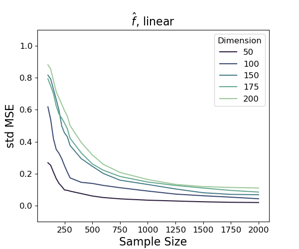
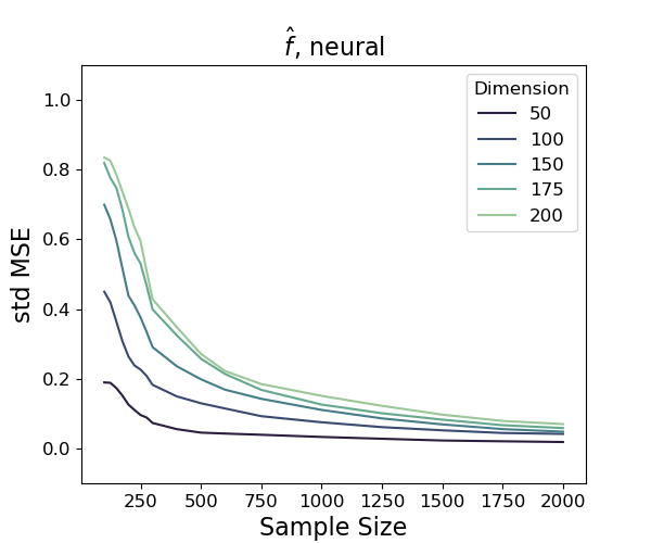
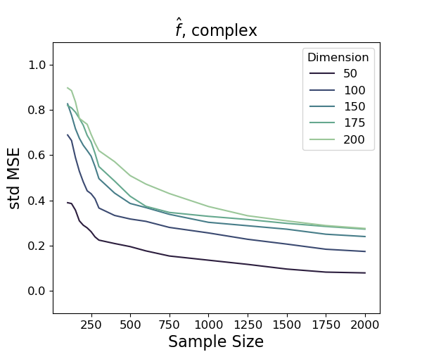
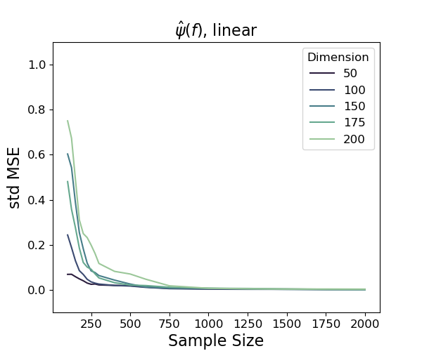
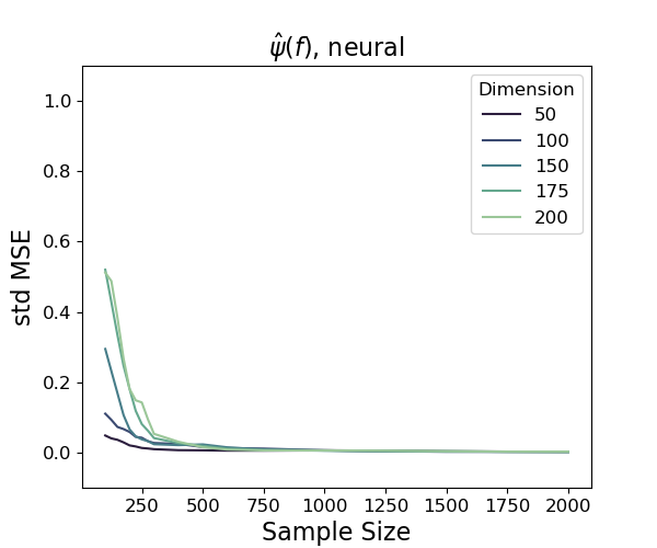
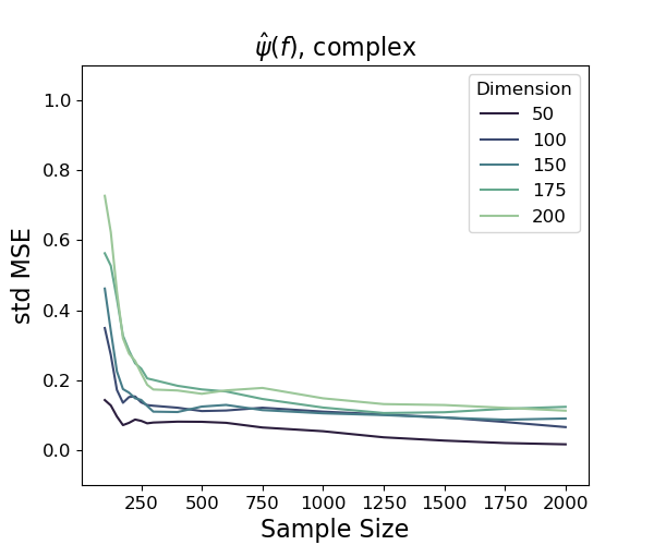
We generate data under the Gaussian noise model $y\sim N(f^{*},1)$ for data-generation function $f^{*}$ with true dimension $P^{*}=5$. We vary the dimension of the data between $P\in(25,200)$, and vary sample sizes $n\in(100,2000)$. For the neural network model, we consider a 2-layer, 50-hidden-unit feed-forward architecture (i.e., $L=2$ and $K=50$) with standard i.i.d. Gaussian priors $N(0,\sigma^{2}=0.1)$ for model weights. We consider three types of data-generating $f^{*}$: (1) linear: a simple linear model $f^{*}(\bx)=\bx^{\top}\bbeta$; (2) neural: a function $f^{*}\in\Fsc(L,W,S,B)$, and (3) complex: a complex, non-smooth multivariate function that is outside the neural network model’s approximation space $\Fsc(L,W,S,B)$. This latter data-generating model violates the assumption that $f^{*}\in\Fsc$ in Proposition 1. We repeat the simulation 20 times for each setting, and evaluate the neural network’s performance in learning $f$ and $\psi_{p}(f)$ using out-of-sample standardized mean squared error (MSE), as follows:

$$std\_MSE(f,f^{*})=$$

$$\quad\Big{[}\frac{1}{n}\sum_{i=1}^{n}[f(\bx_{i})-f^{*}(\bx_{i})]^{2}\Big{]}\Big{/}\Big{[}\frac{1}{n}\sum_{i=1}^{n}[f^{*}(\bx_{i})-E(f^{*}(\bx_{i}))]^{2}\Big{]}.$$

This is essentially the $1-R^{2}$ statistic in regression modeling whose value lies within $(0,1)$. Use of this statistic allows us to directly compare model performance across different data settings. The $std\_MSE$ for $\psi(f)=\{\psi_{p}(f)\}_{p=1}^{P}$ is computed similarly by averaging over all $p\in\{1,\dots,P\}$.

Figure 1 summarizes the standardized MSE s for learning $f^{*}$ and $\psi(f^{*})$, where each column corresponds to a data-generation machanism (linear, neural and complex). The first row summarizes the model’s convergence behavior in prediction (learning $f^{*}$). We see that the model’s learning speed deteriorates as the data dimension $P$ increases. However, this impact of dimensionality appears to be much smaller in the linear and neural scenarios, which both satisfy $f^{*}\in\Fsc$ (Proposition 1). Comparatively, on the second row, the model’s learning speed for variable importance are upper bounded by, and in fact much faster than, the speed of learning $f^{*}$. This verifies our conclusion in Theorem 1 that a model’s good behavior in prediction translates to good performance in learning variable importance. We also observe that when the assumption $f^{*}\in\Fsc$ is violated (e.g. for complex $f^{*}$ in Column 3), the posterior estimate of $\psi_{p}(f)$ still converges toward $\psi_{p}(f_{0})$, although at a rate that is much slower and is more sensitive to the dimension $P$ of the data.

Bernstein-von Mises Phenonmenon

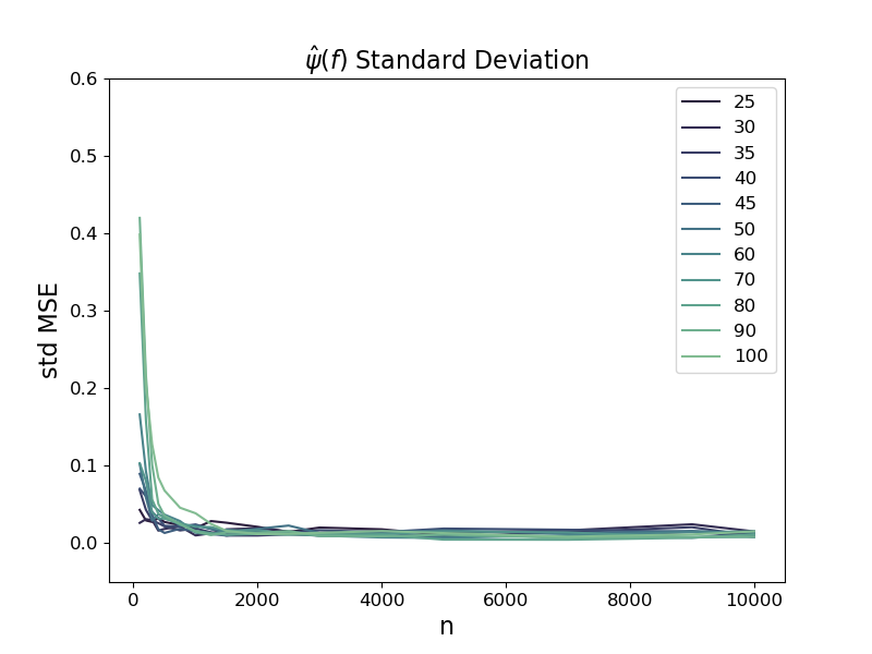
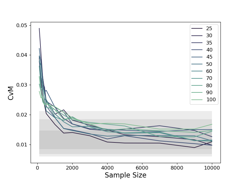
We evaluate the BNN model’s convergence behavior toward the asymptotic posterior $N(0,\sigma_{\texttt{BvM}}^{2}=4||H_{p}\,f_{0}||_{n}^{2})$ using two metrics: (1) the standardized MSE for learning the standard deviation $\sigma_{\texttt{BvM}}$, which assesses whether the spread of the posterior distribution is correct. (2) The Cramér von Mises (CvM) statistic as defined as the empirical $L_{2}$ distance between the standardized posterior sample $\{\psi^{c}_{std,m}\}_{m=1}^{M}$ and a Gaussian distribution $\Phi$. This latter statistic, $CvM(\psi^{c}_{std})=\frac{1}{M}\sum_{m=1}^{M}\big{[}\Fbb(\psi^{c}_{std,m})-\Phi(\psi^{c}_{std,m})\big{]}^{2}$, assesses whether the shape of the posterior distribution is sufficiently symmetric and has a Gaussian tail. Notice that since the CvM is a quadratic statistic, it roughly follows a mixture of $\chi^{2}$ distribution even if true variable importance $\psi(f)$ is zero. Therefore, we compare it against a null distribution of $CvM(\psi^{c}_{std})$ for which $\psi^{c}_{std,m}$ is sampled from a Gaussian distribution.

Figure 2 in the Appendix summarizes the posterior distribution’s convergence behavior in standard deviation (measured by $std\_MSE$, top) and in normality (measured by $CvM$, bottom). The shaded region in the lower figure corresponds to the quantiles of a null CvM distribution. The figure shows that, as the sample size increases, the standardized MSE between $sd(\psi^{c})$ and $\sigma_{BvM}$ converges toward 0, and the CvM statistics enters into the range of the null distribution. The speed of convergence deteriorates as the dimension of the data increases, although not dramatically. These observations indicate that the credible intervals from the variable importance posterior $\Pi_{n}(\psi^{c}(f))$ indeed achieve the correct spread and shape in reasonably large samples, i.e. the Bernstein-von Mises phenomenon holds under the neural network model.

4.2 Effectiveness in High-dimensional Variable Selection

Finally, we study the effectiveness of the proposed variable selection approach (neural variable selection using credible intervals) by comparing it against nine existing methods based on various models (linear-LASSO, random forest, neural network) and decision rules (heuristic thresholding, hypothesis testing, Knockoff). We consider both low- and high-dimension situations ($d\in\{25,75,200\}$) and observe how the performance of each variable selection method changes as the sample size grows.

Table 1: Summary of variable selection methods included in the empirical study.

Model / Metric Decision Rule Thresholding Hypothesis Test Knockoff Linear Model - LASSO Tibshirani (1996) [47] Barber and Candés (2015) [7] Lockhart et al. (2013)[31] Random Forrest - Impurity Breiman (2001)[11] Candés et al. (2018)[13] Altmann et al. (2010)[3] Group $L_{1}$ Thresholding Spike-and-Slab Probability Credible Interval Neural Network - $\Wsc_{1}$ Feng and Simon (2018) [17] Liang et al. (2018) [30] Neural Network - $\psi^{c}(f)$ (this work)

For the candidate variable selection methods, we notice that a variable selection method usually consists of three components: model, measure of variable importance, and the variable-selection decision rule. To this end, we consider nine methods that span three types of models and three types of decision rules (See Table 1 for a summary). The models we consider are (1) LASSO, the classic linear model $y=\sum_{p=1}^{P}x_{p}\beta_{p}$ with LASSO penalty on regression coefficients $\bbeta$, whose variable importance is measured by the magnitude of $\beta_{p}$. (2) RF, the random forest model that measures variable importance using impurity, i.e., the decrease in regression error due to inclusion of a variable $x_{p}$ [11]. (3) NNet, the (deep) neural networks that measure feature importance using either the magnitude of the input weights $\Wsc_{1}$ or, in our case, the integrated gradient norm $\psi^{c}(f)$. For LASSO and RF, we consider three types of decision rule: (1) Heuristic Thresholding, which selects a variable by inspecting if the estimate of $\hat{\beta}_{p}$ is 0 or if the impurity for that variable is greater than $1\%$ of the total impurity summed over all variables [53]; (2) Knockoff, a nonparametric inference procedure that controls the FDR by constructing a data-adaptive threshold for variable importance [13], and (3) Hypothesis Test, which conducts either an asymptotic test on a LASSO-regularized $|\beta_{p}|$ estimate [31] or permutation-based test based on random forest impurity [3], For both of these, we perform the standard Bonferroni correction. We select the LASSO hyper-parameters $\lambda$ based on 10-fold cross validation, and use 500 regression trees for RF. For NNet, we also consider three decision rules: the frequentist approach with group-$L_{1}$ regularization on input weights $\Wsc_{1}$ [17], a Bayesian approach with spike-and-slab priors on $\Wsc_{1}$ [30], and our approach that is based on $95\%$ posterior credible intervals of $\psi_{p}^{c}(f)$. Regarding the NNet architecture, we use $L=1,W=5$ for the LASSO- and Spike-and-slab-regularized networks as suggested by the original authors[17, 30]. We use $L=1,W=50$ for our approach since it is an architecture that is more common in practice.

We generate data by sampling the true function from the neural network model $f^{*}\in\Fsc(L^{*}=1,W^{*}=5)$. Notice that this choice puts our method at a disadvantage compared to other NNets methods, since our network width $W=50>W^{*}$. We fix the number of data-generating covariates to be $d^{*}=5$, and perform variable selection on input features $\bX_{n\times P}$ with dimension $P\in\{25,75,200\}$ which corresponds to low-, moderate-, and high-dimensional situations. We vary sample size $n\in(250,500)$. For each simulation setting $(n,P)$, we repeat the experiment 20 times, and summarize each method’s variable selection performance using the $F_{1}$ score, defined as the geometric mean of variable selection precision $prec=|\hat{S}\cap S|/|\hat{S}|$ and recall $recl=|\hat{S}\cap S|/|S|$ for $S$ the set of data-generating variables and $\hat{S}$ the set of model-selected variables.

Table 2: $F_{1}$ score for classic and machine-learning based variable selection methods (summarized in Table 1) under low-dimension (d=25), moderate-dimension (d=75) and high-dimension data (d=200). Boldface indicates the best-performing decision rules in each dimension-model combination.

Model Rule n=250 n=300 n=350 n=400 n=450 n=500 d=25 LASSO thres $0.65\pm 0.11$ $0.64\pm 0.06$ $0.63\pm 0.08$ $0.76\pm 0.11$ $0.72\pm 0.09$ $0.73\pm 0.06$ knockoff $0.99\pm 0.02$ $0.99\pm 0.04$ $0.94\pm 0.09$ $0.98\pm 0.04$ $0.99\pm 0.03$ $0.99\pm 0.04$ test $1.00\pm 0.00$ $1.00\pm 0.00$ $1.00\pm 0.00$ $0.89\pm 0.00$ $1.00\pm 0.00$ $1.00\pm 0.00$ RF thres $1.00\pm 0.00$ $1.00\pm 0.00$ $1.00\pm 0.00$ $1.00\pm 0.00$ $1.00\pm 0.00$ $1.00\pm 0.00$ knockoff $0.62\pm 0.48$ $1.00\pm 0.02$ $0.96\pm 0.16$ $0.90\pm 0.30$ $0.94\pm 0.19$ $0.99\pm 0.03$ test $0.91\pm 0.05$ $0.98\pm 0.05$ $1.00\pm 0.00$ $0.98\pm 0.05$ $0.98\pm 0.05$ $0.98\pm 0.05$ NNet Group $L_{1}$ $1.00\pm 0.00$ $1.00\pm 0.00$ $1.00\pm 0.00$ $1.00\pm 0.00$ $1.00\pm 0.00$ $1.00\pm 0.00$ SpikeSlab $0.68\pm 0.05$ $0.68\pm 0.05$ $0.70\pm 0.06$ $0.69\pm 0.07$ $0.71\pm 0.08$ $0.72\pm 0.13$ CI (ours) $0.90\pm 0.04$ $0.97\pm 0.05$ $0.98\pm 0.04$ $0.97\pm 0.05$ $0.93\pm 0.06$ $1.00\pm 0.00$ n=250 n=300 n=350 n=400 n=450 n=500 d=75 LASSO thres $0.32\pm 0.04$ $0.31\pm 0.03$ $0.31\pm 0.06$ $0.46\pm 0.11$ $0.56\pm 0.00$ $0.53\pm 0.11$ knockoff $0.93\pm 0.14$ $0.90\pm 0.14$ $0.89\pm 0.15$ $0.94\pm 0.08$ $0.94\pm 0.11$ $0.98\pm 0.04$ test $0.75\pm 0.03$ $0.83\pm 0.07$ $0.91\pm 0.00$ $0.66\pm 0.33$ $0.71\pm 0.00$ $0.89\pm 0.00$ RF thres $0.66\pm 0.10$ $0.67\pm 0.06$ $0.72\pm 0.10$ $0.68\pm 0.06$ $0.80\pm 0.04$ $0.86\pm 0.04$ knockoff $0.79\pm 0.37$ $0.93\pm 0.14$ $0.93\pm 0.17$ $0.92\pm 0.18$ $0.95\pm 0.09$ $0.98\pm 0.05$ test $0.89\pm 0.12$ $0.93\pm 0.07$ $0.86\pm 0.04$ $0.88\pm 0.07$ $0.90\pm 0.09$ $0.95\pm 0.05$ NNet Group $L_{1}$ $0.77\pm 0.00$ $0.67\pm 0.27$ $0.68\pm 0.23$ $0.77\pm 0.00$ $0.77\pm 0.00$ $0.77\pm 0.00$ SpikeSlab $0.63\pm 0.09$ $0.66\pm 0.06$ $0.65\pm 0.08$ $0.65\pm 0.06$ $0.67\pm 0.07$ $0.68\pm 0.10$ CI (ours) $0.98\pm 0.04$ $0.97\pm 0.04$ $0.91\pm 0.07$ $0.97\pm 0.04$ $0.98\pm 0.05$ $1.00\pm 0.00$ n=250 n=300 n=350 n=400 n=450 n=500 d=200 LASSO thres $0.29\pm 0.05$ $0.32\pm 0.01$ $0.28\pm 0.05$ $0.38\pm 0.10$ $0.42\pm 0.08$ $0.35\pm 0.06$ knockoff $0.31\pm 0.42$ $0.68\pm 0.38$ $0.88\pm 0.21$ $0.89\pm 0.11$ $0.90\pm 0.09$ $0.87\pm 0.18$ test $0.21\pm 0.04$ $0.25\pm 0.03$ $0.04\pm 0.00$ $0.49\pm 0.02$ $0.27\pm 0.13$ $0.61\pm 0.04$ RF thres $0.37\pm 0.02$ $0.42\pm 0.01$ $0.43\pm 0.06$ $0.52\pm 0.02$ $0.54\pm 0.05$ $0.59\pm 0.05$ knockoff $0.12\pm 0.25$ $0.29\pm 0.39$ $0.38\pm 0.42$ $0.70\pm 0.42$ $0.80\pm 0.39$ $0.44\pm 0.49$ test $0.79\pm 0.10$ $0.81\pm 0.13$ $0.79\pm 0.07$ $0.87\pm 0.11$ $0.83\pm 0.09$ $0.70\pm 0.08$ NNet Group $L_{1}$ $0.67\pm 0.00$ $0.67\pm 0.00$ $0.67\pm 0.00$ $0.67\pm 0.00$ $0.67\pm 0.00$ $0.67\pm 0.00$ SpikeSlab $0.45\pm 0.26$ $0.53\pm 0.17$ $0.57\pm 0.14$ $0.60\pm 0.14$ $0.57\pm 0.12$ $0.57\pm 0.11$ CI (ours) $0.84\pm 0.10$ $0.76\pm 0.08$ $0.84\pm 0.08$ $0.93\pm 0.07$ $0.98\pm 0.04$ $0.92\pm 0.08$

Table 2 summarizes the performance as quantified by the $F1$ score of the variable-selection methods in low-, medium- and high-dimension situations. In general, we observe that across all methods, LASSO-knockoff, RF-test and our proposed NNet-CI tend to have good performance, with NNet-CI being more effective in higher dimensions (d=200).

Our central conclusion is that a powerful model alone is not sufficient to guarantee effective variable selection. A good measure of variable importance, in terms of an unbiased and low-variance estimator of the true variable importance, and also a rigorous decision rule that has performance guarantee in terms of control over FDR or Type-I error are equally important. For example, although based on a neural network that closely matches the truth, NNet-Group $L_{1}$ and NNet-SpikeSlab measures variable importance using the input weight $\widehat{\Wsc}_{1}$, which is an unstable estimate of variable importance due to over-parametrization and/or non-identifiablity. As a result, the performance of these two models are worse than the linear-model based LASSO-knockoff. Comparing between the decision rules, the heuristic thresholding rules (LASSO-thres and RF-thres) are mostly not optimized for variable selection performance. As a result, they tend to be susceptible to the multiple comparison problem and their performance deteriorates quickly as the dimension increases. The Knockoff-based methods (LASSO-knockoff and RF-knockoff) are nonparametric procedures that are robust to model misspecification but tend to have weak power when the model variance is high. As a result, the Knockoff approach produced good results for the low-variance linear-LASSO model, but comparatively worse result for the more flexible but high-variance random forest model. Finally, the hypothesis tests / credible intervals are model-based procedures whose performance depends on the quality of the model. Hypothesis tests are expected to be more powerful when the model yields an unbiased and low-variance estimate of $f^{*}$ (i.e. RF-test and NNet-CI), but has no performance guarantee when the model is misspecified (i.e. LASSO). In summary, we find that the NNet-CI method combines a powerful model that is effective in high dimension with a good variable-importance measure that has fast rate of convergence and also a credible-based selection rule that has a rigorous statistical guarantee. As a result, even without any sparse-inducing model regularization, NNet-CI out-performed its NNet-based peers, and is more powerful than other LASSO- or RF-based approaches in high dimensions.

5 Discussion and Future Directions

In this work, we investigate the theoretical basis underlying the deep BNN’s ability to achieve rigorous uncertainty quantification in variable selection. Using the square integrated gradient $\psi_{p}(f)=||\deriv{x_{p}}f||_{n}^{2}$ as the measure of variable importance, we established two new Bayesian nonparametric results on the BNN’s ability to learn and quantify uncertainty about variable importance. Our results suggest that the neural network can learn variable importance effectively in high dimensions (Theorem 1), in a speed that in some cases “breaks” the curse of dimensionality (Proposition 1). Moreover, it can generate rigorous and calibrated uncertainty estimates in the sense that its $(1-q)$-level credible intervals for variable importance cover the true parameter $(1-q)\%$ of the time (Theorem 2-3). The simulation experiments confirmed these theoretical findings, and revealed the interesting fact that BNN can learn variable importance $\psi_{p}(f)$ at a rate much faster than learning predictions for $f^{*}$ (Figure 1). The comparative study illustrates the effectiveness of the proposed approach for the purpose of variable selection in high dimensions, which is a scenario where the existing methods experience difficulties due to model misspecification, the curse of dimensionality, or the issue of multiple comparisons.

Consistent with classic Bayesian nonparametric and deep learning literature [15, 39, 8, 9], the theoretical results developed in this work assume a well-specified scenario where $f^{*}\in\Fsc$ and the noise distribution is known. Furthermore, computing exact credible intervals under a BNN model requires the use of MCMC procedures, which can be infeasible for large datasets. Therefore two important future directions of this work are to investigate the BNN’s ability to learn variable importance under model misspecification, and to identify posterior inference methods (e.g., particle filter [16] or structured variational inference [37]) that are scalable to large datasets and can also achieve rigorous uncertainty quantification.

Appendix A Statement of Multivariate BvM Theorem

Theorem 3 (Multivariate Bernstein-von Mises (BvM) for $\psi^{c}$).

For $f\in\Fsc(L,W,S,B)$, assuming the posterior distribution $\Pi_{n}(f)$ contracts around $f_{0}$ at rate $\epsilon_{n}$. Denote $\hat{\psi}^{c}=[\hat{\psi}^{c}_{1},\dots,\hat{\psi}^{c}_{P}]$ for $\hat{\psi}^{c}_{p}$ as defined in Theorem 2. Also recall that $P=o(1)$, i.e. the data dimension does not grow with sample size.

Then $\hat{\psi}^{c}$ is an unbiased estimator of $\psi(f_{0})=[\psi_{1}(f_{0}),\dots,\psi_{P}(f_{0})]$, and the posterior distribution for $\psi^{c}(f)$ asymptotically converge toward a multivariate normal distribution surrounding $\hat{\psi}^{c}$, i.e.

$$\Pi\Big{(}\sqrt{n}(\psi^{c}(f)-\hat{\psi}^{c})\Big{|}\{\bx_{i},y_{i}\}_{i=1}^{n}\Big{)}\leadsto MVN(0,V_{0}),$$

where $V_{0}$ is a $P\times P$ matrix such that $(V_{0})_{p_{1},p_{2}}=4\langle H_{p_{1}}f_{0},H_{p_{2}}f_{0}\rangle_{n}$.

Proof is in Supplementary Section LABEL:sec:bvm_mvn_proof.

Appendix B Table and Figures

(a)

(b)

Figure 2: The variable importance posterior’s convergence behavior toward the asymptotic standard deviation (left, measured by standardized MSE) and toward normality (right, measured by the CvM distance from a Gaussian distribution) under sample size $n\in(100,10000)$ and $P\in(25,100)$. Shaded region in the right figure indicates the $\{5\%,10\%,25\%,75\%,90\%,95\%\}$ quantiles of the null CvM distribution.

References

- [1] M. Abadi, P. Barham, J. Chen, Z. Chen, A. Davis, J. Dean, M. Devin, S. Ghemawat, G. Irving, M. Isard, M. Kudlur, J. Levenberg, R. Monga, S. Moore, D. G. Murray, B. Steiner, P. Tucker, V. Vasudevan, P. Warden, M. Wicke, Y. Yu, and X. Zheng. TensorFlow: A system for large-scale machine learning. arXiv:1605.08695 [cs], May 2016. arXiv: 1605.08695.
- [2] R. A. Adams and J. J. F. Fournier. Sobolev Spaces, Volume 140. Academic Press, Amsterdam, 2 edition edition, July 2003.
- [3] A. Altmann, L. Toloşi, O. Sander, and T. Lengauer. Permutation importance: a corrected feature importance measure. Bioinformatics, 26(10):1340–1347, May 2010.
- [4] U. Anders and O. Korn. Model selection in neural networks. Neural Networks, 12(2):309–323, Mar. 1999.
- [5] C. Andrieu and J. Thoms. A tutorial on adaptive MCMC. Statistics and Computing, 18(4):343–373, Dec. 2008.
- [6] F. Bach. Breaking the Curse of Dimensionality with Convex Neural Networks. arXiv:1412.8690 [cs, math, stat], Dec. 2014. arXiv: 1412.8690.
- [7] R. F. Barber and E. J. Candès. Controlling the false discovery rate via knockoffs. The Annals of Statistics, 43(5):2055–2085, Oct. 2015.
- [8] A. R. Barron. Universal approximation bounds for superpositions of a sigmoidal function. IEEE Transactions on Information Theory, 39(3):930–945, May 1993.
- [9] A. R. Barron and J. M. Klusowski. Approximation and Estimation for High-Dimensional Deep Learning Networks. arXiv:1809.03090 [cs, stat], Sept. 2018. arXiv: 1809.03090.
- [10] Y. Benjamini and Y. Hochberg. Controlling the False Discovery Rate: A Practical and Powerful Approach to Multiple Testing. Journal of the Royal Statistical Society. Series B (Methodological), 57(1):289–300, 1995.
- [11] L. Breiman. Random Forests. Machine Learning, 45(1):5–32, Oct. 2001.
- [12] P. Bühlmann. Statistical significance in high-dimensional linear models. Bernoulli, 19(4):1212–1242, Sept. 2013.
- [13] E. Candès, Y. Fan, L. Janson, and J. Lv. Panning for gold: ‘model-X’ knockoffs for high dimensional controlled variable selection. Journal of the Royal Statistical Society: Series B (Statistical Methodology), 80(3), June 2018.
- [14] G. Castellano and A. M. Fanelli. Variable selection using neural-network models. Neurocomputing, 31(1):1–13, Mar. 2000.
- [15] I. Castillo and J. Rousseau. A Bernstein–von Mises theorem for smooth functionals in semiparametric models. The Annals of Statistics, 43(6):2353–2383, Dec. 2015.
- [16] B. Dai, N. He, H. Dai, and L. Song. Provable Bayesian Inference via Particle Mirror Descent. In Artificial Intelligence and Statistics, pages 985–994, May 2016.
- [17] J. Feng and N. Simon. Sparse Input Neural Networks for High-dimensional Nonparametric Regression and Classification. arXiv:1711.07592 [stat], Nov. 2017. arXiv: 1711.07592.
- [18] A. Gelman, J. Hill, and M. Yajima. Why We (Usually) Don’t Have to Worry About Multiple Comparisons. Journal of Research on Educational Effectiveness, 5(2):189–211, Apr. 2012.
- [19] S. Ghosal and A. van der Vaart. Convergence rates of posterior distributions for noniid observations. The Annals of Statistics, 35(1):192–223, Feb. 2007.
- [20] S. Ghosh and F. Doshi-Velez. Model Selection in Bayesian Neural Networks via Horseshoe Priors. arXiv:1705.10388 [stat], May 2017. arXiv: 1705.10388.
- [21] F. Giordano, M. L. Rocca, and C. Perna. Input Variable Selection in Neural Network Models. Communications in Statistics - Theory and Methods, 43(4):735–750, Feb. 2014.
- [22] R. Gribonval, G. Kutyniok, M. Nielsen, and F. Voigtlaender. Approximation spaces of deep neural networks. arXiv:1905.01208 [cs, math, stat], May 2019. arXiv: 1905.01208.
- [23] I. Guyon and A. Elisseeff. An Introduction to Variable and Feature Selection. Journal of Machine Learning Research, 3(Mar):1157–1182, 2003.
- [24] K. He, X. Zhang, S. Ren, and J. Sun. Deep Residual Learning for Image Recognition. In 2016 IEEE Conference on Computer Vision and Pattern Recognition (CVPR), pages 770–778, June 2016.
- [25] X. He, J. Wang, and S. Lv. Scalable kernel-based variable selection with sparsistency. arXiv:1802.09246 [cs, stat], Feb. 2018. arXiv: 1802.09246.
- [26] A. Krizhevsky, I. Sutskever, and G. E. Hinton. ImageNet Classification with Deep Convolutional Neural Networks. In F. Pereira, C. J. C. Burges, L. Bottou, and K. Q. Weinberger, editors, Advances in Neural Information Processing Systems 25, pages 1097–1105. Curran Associates, Inc., 2012.
- [27] M. La Rocca and C. Perna. Variable selection in neural network regression models with dependent data: a subsampling approach. Computational Statistics & Data Analysis, 48(2):415–429, Feb. 2005.
- [28] Y. LeCun, J. S. Denker, and S. A. Solla. Optimal Brain Damage. In D. S. Touretzky, editor, Advances in Neural Information Processing Systems 2, pages 598–605. Morgan-Kaufmann, 1990.
- [29] H. K. Lee. Consistency of posterior distributions for neural networks. Neural Networks: The Official Journal of the International Neural Network Society, 13(6):629–642, July 2000.
- [30] F. Liang, Q. Li, and L. Zhou. Bayesian Neural Networks for Selection of Drug Sensitive Genes. Journal of the American Statistical Association, 113(523):955–972, July 2018.
- [31] R. Lockhart, J. Taylor, R. Tibshirani, and R. Tibshirani. A significance test for the LASSO. The Annals of Statistics, 42, Jan. 2013.
- [32] C. Louizos, M. Welling, and D. P. Kingma. Learning Sparse Neural Networks through L_0 Regularization. Feb. 2018.
- [33] Y. Y. Lu, Y. Fan, J. Lv, and W. S. Noble. DeepPINK: reproducible feature selection in deep neural networks. Sept. 2018.
- [34] R. May, G. Dandy, and H. Maier. Review of Input Variable Selection Methods for Artificial Neural Networks. Artificial Neural Networks - Methodological Advances and Biomedical Applications, Apr. 2011.
- [35] H. Montanelli and Q. Du. New error bounds for deep networks using sparse grids. arXiv:1712.08688 [math], Dec. 2017. arXiv: 1712.08688.
- [36] R. M. Neal. Bayesian Learning for Neural Networks. Lecture Notes in Statistics. Springer-Verlag, New York, 1996.
- [37] M. F. Pradier, W. Pan, J. Yao, S. Ghosh, and F. Doshi-velez. Projected BNNs: Avoiding weight-space pathologies by learning latent representations of neural network weights. arXiv:1811.07006 [cs, stat], Nov. 2018. arXiv: 1811.07006.
- [38] V. Rockova and N. Polson. Posterior Concentration for Sparse Deep Learning. In S. Bengio, H. Wallach, H. Larochelle, K. Grauman, N. Cesa-Bianchi, and R. Garnett, editors, Advances in Neural Information Processing Systems 31, pages 930–941. Curran Associates, Inc., 2018.
- [39] V. Rockova and E. Saha. On Theory for BART. arXiv:1810.00787 [cs, stat], Oct. 2018. arXiv: 1810.00787.
- [40] L. Rosasco, S. Villa, S. Mosci, M. Santoro, and A. Verri. Nonparametric Sparsity and Regularization. Journal of Machine Learning Research, 14:1665–1714, 2013.
- [41] O. Russakovsky, J. Deng, H. Su, J. Krause, S. Satheesh, S. Ma, Z. Huang, A. Karpathy, A. Khosla, M. Bernstein, A. C. Berg, and L. Fei-Fei. ImageNet Large Scale Visual Recognition Challenge. International Journal of Computer Vision, 115(3):211–252, Dec. 2015.
- [42] S. Scardapane, D. Comminiello, A. Hussain, and A. Uncini. Group sparse regularization for deep neural networks. Neurocomputing, 241:81–89, June 2017.
- [43] J. Schmidt-Hieber. Nonparametric regression using deep neural networks with ReLU activation function. arXiv:1708.06633 [cs, math, stat], Aug. 2017. arXiv: 1708.06633.
- [44] K. Simonyan and A. Zisserman. Very Deep Convolutional Networks for Large-Scale Image Recognition. arXiv:1409.1556 [cs], Sept. 2014. arXiv: 1409.1556.
- [45] T. Suzuki. Adaptivity of deep ReLU network for learning in Besov and mixed smooth Besov spaces: optimal rate and curse of dimensionality. Sept. 2018.
- [46] C. Szegedy, V. Vanhoucke, S. Ioffe, J. Shlens, and Z. Wojna. Rethinking the Inception Architecture for Computer Vision. 2016 IEEE Conference on Computer Vision and Pattern Recognition (CVPR), pages 2818–2826, 2015.
- [47] R. Tibshirani. Regression Shrinkage and Selection via the Lasso. Journal of the Royal Statistical Society. Series B (Methodological), 58(1):267–288, 1996.
- [48] A. W. van der Vaart. Asymptotic Statistics. Cambridge University Press, Cambridge, June 2000.
- [49] G. Wahba. Spline Models for Observational Data. SIAM, Sept. 1990. Google-Books-ID: ScRQJEETs0EC.
- [50] H. White and J. Racine. Statistical inference, the bootstrap, and neural-network modeling with application to foreign exchange rates. IEEE Transactions on Neural Networks, 12(4):657–673, July 2001.
- [51] L. Yang, S. Lv, and J. Wang. Model-free Variable Selection in Reproducing Kernel Hilbert Space. Journal of Machine Learning Research, 17(82):1–24, 2016.
- [52] D. Yarotsky. Error bounds for approximations with deep ReLU networks. arXiv:1610.01145 [cs], Oct. 2016. arXiv: 1610.01145.
- [53] M. Ye and Y. Sun. Variable Selection via Penalized Neural Network: a Drop-Out-One Loss Approach. In International Conference on Machine Learning, pages 5620–5629, July 2018.