Adaptive Online Planning
for Continual Lifelong Learning
Abstract
We study learning control in an online reset-free lifelong learning scenario, where mistakes can compound catastrophically into the future and the underlying dynamics of the environment may change. Traditional model-free policy learning methods have achieved successes in difficult tasks due to their broad flexibility, but struggle in this setting, as they can activate failure modes early in their lifetimes which are difficult to recover from and face performance degradation as dynamics change. On the other hand, model-based planning methods learn and adapt quickly, but require prohibitive levels of computational resources. We present a new algorithm, Adaptive Online Planning (AOP), that achieves strong performance in this setting by combining model-based planning with model-free learning. By approximating the uncertainty of the model-free components and the planner performance, AOP is able to call upon more extensive planning only when necessary, leading to reduced computation times, while still gracefully adapting behaviors in the face of unpredictable changes in the world – even when traditional RL fails.
1 Introduction
We consider agents in a lifelike setting, where agents must simultaneously act and learn in the world continuously with limited computational resources. All decisions are made online; there are no discrete episodes. Furthermore, the world is vast – too large to feasibly explore exhaustively – and changes over the course of the agent’s lifetime, like how a robot’s actuators might deteriorate with continued use. Mistakes are costly, as they compound downstream; there are no resets to wipe away past errors. To perform well at reasonable computational costs, the agent must utilize its past experience alongside new information about the world to make careful, yet performant, decisions.
Non-stationary worlds require algorithms that are fundamentally robust to changes in dynamics. Factors that would lead to a change in the environment may either be too difficult or principally undesirable to model: for example, humans might interact with the robot in unpredictable ways, or furniture in a robot’s environment could be rearranged. Therefore, we assume that the world can change unpredictably in ways that cannot be learned, and focus on developing algorithms that instead handle these changes gracefully, without using extensive computation.
Model-based planning is useful for quickly learning control, but is computationally demanding and can be biased by the finite planning horizon. Model-free RL is sample inefficient, but capable of cheaply accessing past experience. Consequently, we would like to distill expensive experience generated by a powerful planner into model-free networks to reduce computation. However, deciding on when to use planning versus model-free control is nontrivial. When uncertain about a course of action, humans use an elongated model-based search to evaluate long-term trajectories, but fall back on habitual behaviors learned with model-free paradigms when uncertainty is low evans1984 ; daw2005uncertainty ; dayan2014model ; kahn2003 . By measuring this uncertainty, we can make informed decisions about when to use extensive planning.
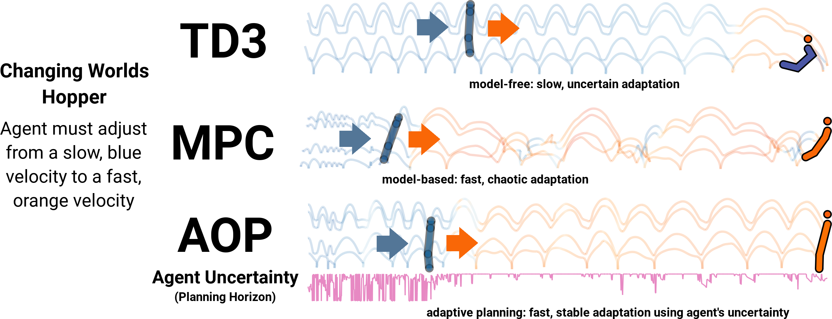
Our approach combines model-based planning with model-free learning, along with an adaptive computation mechanism, to tackle this setting. Like a robot that is well-calibrated when first coming out of a factory, we give the agent access to a ground truth dynamics model that lacks information about future changes to the dynamics, such as different settings in which the robot may be deployed. This allows us to make progress on finite computation continual learning without complications caused by model learning. The dynamics model is updated immediately at world changes. However, as we show empirically, knowing the dynamics alone falls far short of success at this task.
We present a new algorithm, Adaptive Online Planning (AOP), that links model-based planning with model-free policy optimization. We interpolate between the two methods using a unified update rule formulation that is amenable to reduced computation when combined with a switching mechanism. We inform this mechanism with the uncertainty given by an ensemble of value functions. We show that access to the ground truth model is not sufficient by itself, as PPO ppo and TD3 td3 perform poorly, even with such a model. In particular, we discover that policy-based methods degrade in performance over time as the world changes. We provide intuition, qualitative analysis, and demonstrate empirically that AOP is capable of integrating the two methodologies to reduce computation while achieving and maintaining strong performance in non-stationary worlds, outperforming other model-based planning methods and avoiding the performance degradation of policy learning methods.
2 Background
2.1 Notation and Setting
We consider the world as an infinite-horizon MDP defined by the tuple , where is the state space, is the action space, is the reward function, are the transition probabilities, and is the discount factor. The world changes over time: may switch to new at multiple points during training. Unlike traditional RL, the agent’s state is not reset at these world changes, and these changes are not observed in the state. The agent has access to a perfect local model, i.e. it can generate rollouts using the current starting from its current state . It does not have access to future . The agent’s goal is to execute a policy , that maximizes the -horizon expected return as for . We denote the value function .
We consider reset-free online learning to be the setting where both acting and learning must occur on a per-timestep basis, and there are no episodes that reset the state. At each timestep, the agent must execute its training, and is then forced to immediately output an action. The world changes between environments sequentially. Agents should use past experience to perform well in new tasks, while avoiding past negative transfer of experience. In addition to the these adversities, agents must avoid failure sink states that prevent future learning progress, as the agent cannot reset. These challenges yield a difficult setting which more closely parallels a human lifetime than traditional episodic RL.
2.2 Model-Based Planning
Online model-based planning (see Algorithm 1) evaluates future sequences of actions using a model of the environment, develops a projected future trajectory over some time horizon, and then executes the first action of that trajectory, before replanning at the next timestep. We specifically focus on shooting-based Model Predictive Control (MPC). When the update rule is a softmax weighting, this procedure is called Model Predictive Path Integral (MPPI) control mppi . Due to the nature of this iterative and extended update, this procedure is computationally expensive, and can lead to unpredictable and irregular behaviors, as it is a brute-force black box optimizer.
2.3 Model-Free Policy Optimization
Model-free algorithms encode the agent’s past experiences in neural network functions dependent only on the current state, often in the form of a value function critic and/or policy actor. As a result, such algorithms can have difficulty learning long-term dependencies and struggle early on in training; temporally-extended exploration is difficult. In exchange, they attain high asymptotic performance, having shown successes in a variety of tasks in the episodic setting dqn ; ppo . As a consequence of their compact nature, once learned, these algorithms tend to generate cyclic and regular behaviors, whereas model-based planners have no such guarantees (see Figure 1 for an illustration).
We run online versions of TD3 td3 and PPO ppo as baselines to AOP. While there is no natural way to give a policy access to the ground truth model, we allow the policies to train on future trajectories generated via the ground truth model, similarly to model-based policy optimization algorithms steve ; metrpo , in order to help facilitate fair comparisons to model-based planners (see Algorithm 2).
3 Unifying Model-Based Planning and Model-Free Control
3.1 Update Rule Perspective on Model-Based Planning vs Policy Optimization
From a high-level perspective, the model-based planning and model-free policy optimization procedures are very similar (see Algorithms 1 and 2 for a side-by-side comparison). Where the planner generates noisy rollouts to synthesize a new trajectory, the model-free algorithm applies noise to the policy to generate data for learning. After an update step, either an action from the planned trajectory or one call of the policy is executed. These procedures are only distinct in their respective update rules: planning uses a fast update, while policy optimization uses a slow one.
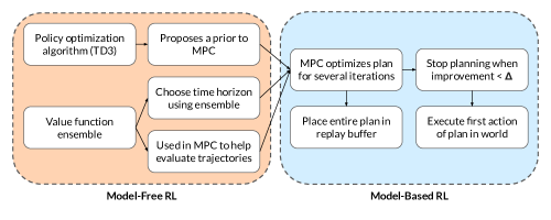
The primary contribution of our algorithm, AOP, is unifying both update rules to compensate for their individual weaknesses. AOP distills the learned experience from the planner into the off-policy learning method of TD3 and a value function, so that planning and acting can be cheaper in the future.
3.2 Model-Based Planning with Terminal Value Approximation
AOP uses MPPI mppi as the planning algorithm, with a learned terminal value function , seeking to optimize the -step objective . This process is repeated for several iterations, and then the first action is executed in the environment. is generated by an ensemble of value functions as , similar to POLO polo . The value ensemble improves the exploration of the optimization procedure rpf ; bs-dqn . The log-sum-exp function serves as a softmax, enabling optimistic exploration. The term normalizes the estimate to lie between the mean and the max of the ensemble, determined by the temperature hyperparameter , ensuring that the approximation is semantically meaningful for value estimation.
Crucially, instead of a fixed horizon, AOP adaptively chooses the planning horizon to interpolate between model-free control (short ) and model-based planning (long ); see Algorithm 3. This planning horizon is set based on the uncertainty of the value function, discussed in Section 4.2.
3.3 Off-Policy Model-Free Prior
We use TD3 td3 as a prior to the planning procedure, with the policy learning off of the data generated by the planner, which allows the agent to recall past experience quickly. Note that we use to distinguish from , which represents the agent as a whole. In line with past work rajeswaran2017learning ; zhu2018reinforcement , we found that imitation learning can cap the asymptotic performance of the learned policy. As a baseline, we also run behavior cloning (BC) as a prior, and refer to the resulting algorithms as AOP-TD3 and AOP-BC.
We note that MPC and policy optimization are both special cases of AOP. MPC is equivalent to AOP with a constant setting for the time horizon that always uses full planning iterations (). Policy optimization is equivalent to AOP with one planning iteration, since the first plan is a noisy version of the policy, acting as the data collection procedure in standard policy learning.
4 Adaptive Planning for Reset-Free Lifelong Learning
4.1 Long-Term Regret in Lifelong Learning
In our setting, we can consider “long-term regret” derived from planning over the model using a limited time horizon. A more formal/detailed version is included in Appendix A.
Definition 4.1.
Let the planning regret denote the suboptimality in the infinite-horizon value of the rollout when using an MPC planner over an -step horizon and executing the policy afterwards vs. planning using an infinite-horizon planner: .
Using a ∗ to denote states generated by an optimal policy/planner, we can rewrite the regret as:
where in the last line we decompose the regret as the sum of the short-term and long-term regret. We focus on the long-term regret term due to how it models our lifelong learning setting.
Lemma 1.
Let the value approximation error be bounded as and the future agent policy suboptimality be bounded as . Then we have:
At a high level, this intuitively poses the long-term regret as the sum of short-term greed, long-term value approximation error, and long-term agent policy suboptimality.
4.1.1 Why Focus on Long-Term Regret?
The notion of long-term regret is particularly important in the reset-free setting, as there exists “pseudo-terminal” sink states where, not only does the agent incur large penalty, but also it is hard to make further learning progress at all. Traditional episodic RL only incurs the large penalty, and does not suffer a block on the learning ability, hence the traditional notion of “long-term” refers to only within the current trajectory, but the reset-free notion of “long-term” refers to the entire training loop, which makes improper handling of long-term regret far more catastrophic. This also corresponds to how we consider to be far shorter than the total lifelong horizon, or similarly or .
Consider the trajectory of TD3 shown in Figure 1. One-step lookahead policy optimization algorithms suffer a high value approximation error at dramatic world changes. At the end of the shown trajectory, the policy optimizes for the short-term ability to achieve the new orange target velocity, in exchange for falling over, which inhibits its ability to continue learning and acting, thereafter suffering a large long-term penalty. While this is not easily modeled by standard notions of regret or the short-term regret, this is captured by the long-term regret, and is a principle cause of policy degradation. To a lesser extent, the MPC trajectory also exhibits this, as it continually greedily optimizes for reward in the near future, matching the target velocity extremely well, but suffering periods of failure where it falls over and does not match the target velocity, though it generally recovers sufficiently.
4.2 Adaptive Planning Horizon
Now, under Lemma 1, we can consider AOP as a tradeoff between these two extremes. In particular, we propose AOP as minimizing given a constraint on the value approximation error/long-term regret, allowing the agent to utilize more model-free control and save computation as long as the value function approximator is accurate. We use two heuristics to approximate the uncertainty:
-
•
The standard deviation of the value function ensemble, which represents the epistemic uncertainty of the value of the state rpf . In particular, we automatically use the full planning horizon if the standard deviation is greater than a threshold .
(1) -
•
The Bellman error of the value (see Equation 1), which directly approximates the error of the value function. In particular, this uncertainty is high in changing worlds, whereas the standard deviation is not. We use the longest such that .
While choices for and are somewhat arbitrary, we show in Appendix D.1 that AOP is not particularly sensitive to them, and they generally transfer between environments.
4.3 Early Planning Termination
Additionally, we save computation by running less planning iterations. Past model-based planning procedures pets ; poplin run a fixed number of iterations of MPC per timestep before executing an action in the environment, which can be wasteful, as later iterations are less useful. Consequently, we propose to decide on the number of planning iterations on a per-timestep basis. After generating a new trajectory from the -th iteration of planning, we measure the improvement against the trajectory of the previous iteration. When this improvement decreases below a threshold , we terminate planning for the current timestep with probability . We find that using a stochastic termination rule allows for more robustness against local minima.
5 Empirical Evaluations
We investigate several questions empirically:
-
1.
What are the challenges in the continual lifelong learning setting? When developing further algorithms in this setting, what should we focus on?
-
2.
How does AOP perform in well-known states, novel states, and in changing worlds scenarios? How do traditional on-policy and off-policy methods fare in these situations?
-
3.
Are the variance and the Bellman error of the value ensemble suitable metrics for representing the agent’s uncertainty and determining the planning computational budget?
5.1 Lifelong Learning Environments
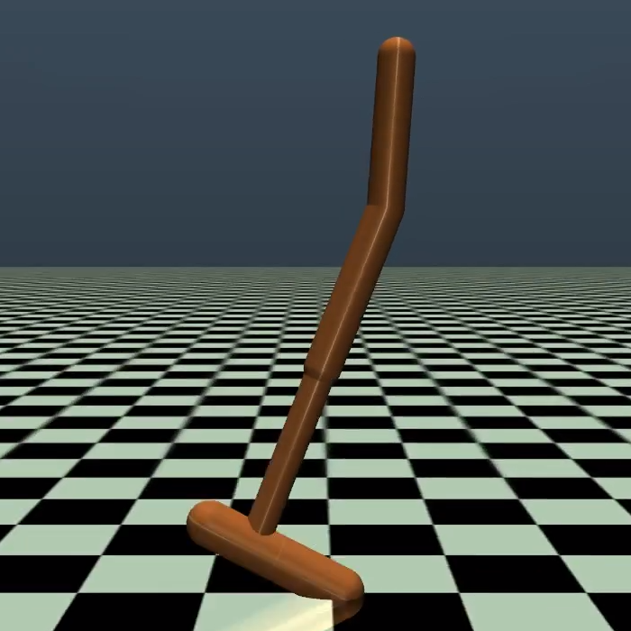
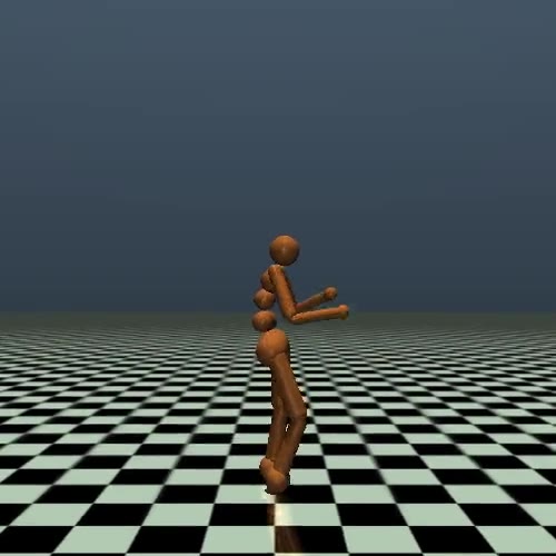
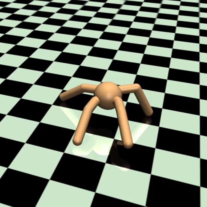
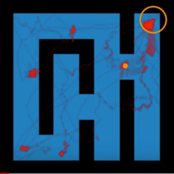
We propose four environments to evaluate our proposed algorithm in the continual lifelong learning setting: Hopper, Humanoid, Ant, and Maze. We consider three classes of experiments: “standard” experiments (S) where the world never changes, which is similar to standard RL except for not having resets; novel states (NS) experiments where the dynamics never changes, but the agent’s assigned task changes and is observed (equating to new states); and changing worlds experiments (CW) – the focus of this work – where the dynamics and/or task will change and not be observed in the state.
Hopper: A hopping agent is rewarded based on how closely its forward velocity matches an unobserved changing target velocity. Long-term regret is extremely poignant in this environment, as the hopping motion can cause long-term value to be sacrificed for short-term reward, and momentum can cause the agent to fall over, after which it can be hard to recover, stifling further learning progress. Hopper is not a difficult control environment, but it is the most unstable environment in this setting. In the novel states setting, the target velocity is included in the observation.
Humanoid: A humanoid agent seeks to achieve a fixed forward velocity, where the mass of its right arm varies greatly during its lifetime. Recovering after falling face-first is extremely difficult.
Ant: A four-legged agent seeks to achieve a fixed forward velocity, where a joint at random is disabled every 2000 timesteps. Again, falling over can hinder learning greatly.
Maze: We test in a 2D continuous point mass maze, where the agent seeks to reach a goal, which is included in the observation. We consider two versions: (1) a novel states Maze, where the walls of the maze remain constant, but new goals are introduced periodically, and (2) a changing worlds Maze, where both the walls and the goal constantly change. We also test both versions in a both a dense reward and a sparse reward setting.
These environments test a variety of challenges a lifelong agent might face: changes in the reward specification (Hopper, Maze), changes in the underlying dynamics parameters (Humanoid), changes in the action space (Ant), and long-term global changes in the world structure (Maze). Furthermore, they each exhibit difficult local optima that can be difficult to recover from in the reset-free setting.
5.2 Baselines and Ablations
We run AOP-BC, POLO, MPC, TD3, and PPO as baselines against AOP-TD3; they can be seen as ablations/special cases of our proposed algorithm. We consider two versions of MPC, with and planning iterations (referred to as MPC-8 and MPC-3), to consider the effect of computation.

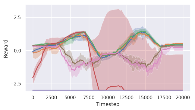
(a) Hopper
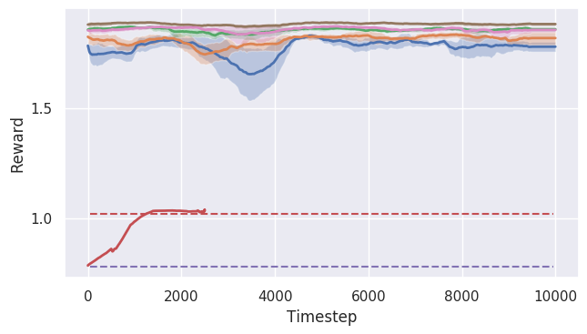
(b) Humanoid
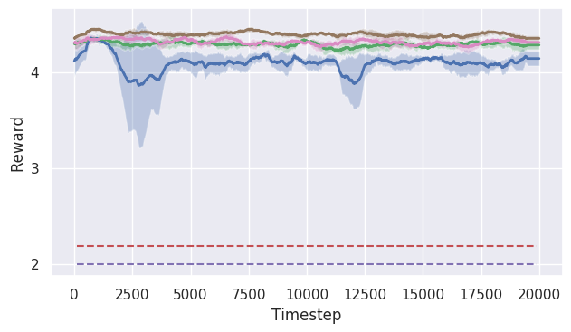
(c) Ant
(d) Maze (D)
| Env | AOP-TD3 | AOP-BC | POLO | TD3 | PPO | MPC-8 | MPC-3 | |
|---|---|---|---|---|---|---|---|---|
| S | Hopper | 0.12 0.16 | 0.33 0.22 | 0.51 | 0.23 | -14.4 | 0.36 | 0.19 |
| NS | Hopper | 0.41 0.18 | 0.53 0.18 | 0.59 | 0.40 | -14.2 | -0.28 | -0.49 |
| CW | Hopper | 0.48 0.24 | 0.45 0.12 | 0.57 | -2.42 | -13.1 | -0.30 | -0.48 |
| S | Human | 1.79 0.02 | 1.80 0.02 | 1.86 | 1.01∗ | 0.78∗ | 1.88 | 1.87 |
| CW | Human | 1.78 0.03 | 1.80 0.02 | 1.85 | 1.01∗ | 0.78∗ | 1.88 | 1.86 |
| S | Ant | 4.15 0.11 | 4.17 0.03 | 4.30 | 2.19 | n/a | 4.41 | 4.34 |
| CW | Ant | 4.10 0.06 | 4.15 0.03 | 4.29 | 2.05 | n/a | 4.40 | 4.32 |
| NS | Maze (D) | -0.21 0.08 | -0.25 0.02 | -0.25 | -1.81 | -2.14 | -0.19 | -0.25 |
| CW | Maze (D) | -0.29 0.07 | -0.34 0.03 | -0.30 | -1.17 | -2.10 | -0.19 | -0.30 |
| NS | Maze (S) | 0.85 0.07 | 0.70 0.06 | 0.62 | -0.68 | -0.88 | 0.69 | 0.61 |
| CW | Maze (S) | 0.69 0.20 | 0.56 0.04 | 0.57 | -0.66 | -0.74 | 0.58 | 0.52 |
| AOP-TD3 | AOP-BC | POLO | MPC-8 | MPC-3 |
|---|---|---|---|---|
| 11.99% (1.40% - 16.62%) | 11.96% (2.86% - 15.17%) | 37.50% | 100% | 37.50% |
5.3 Challenges in Reset-Free Continual Lifelong Learning
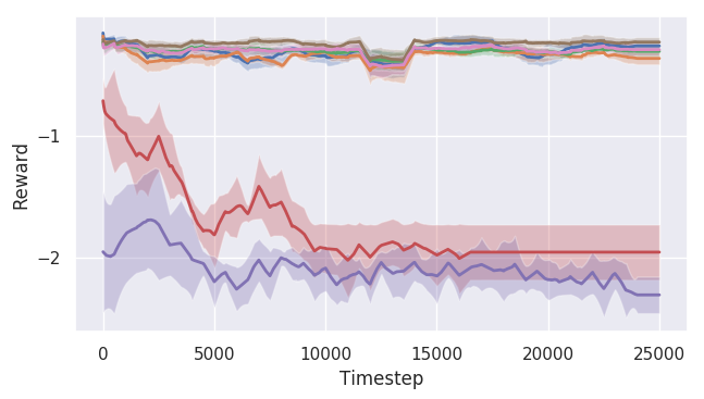
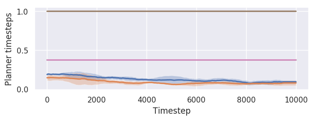
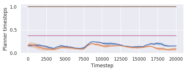
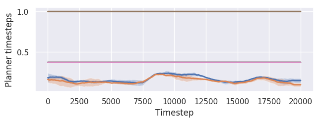
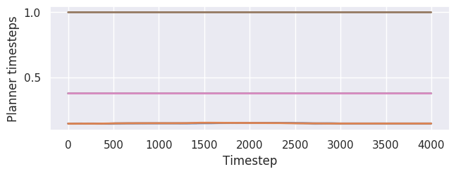
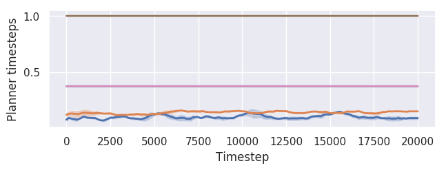
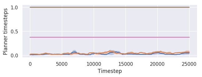
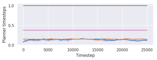
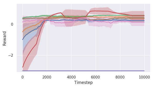
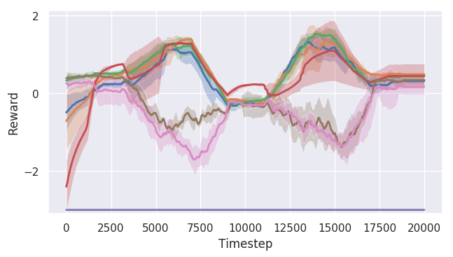
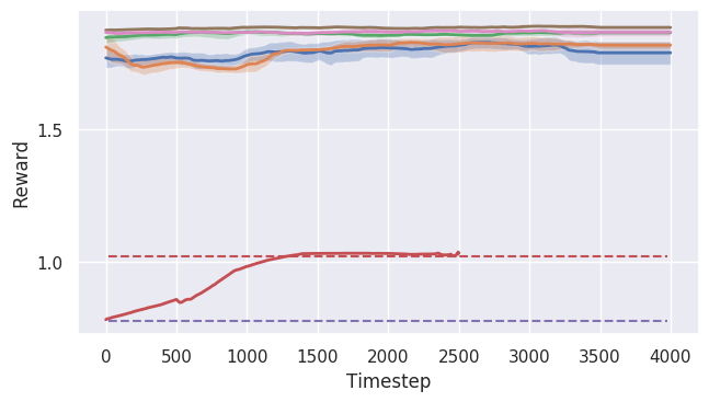
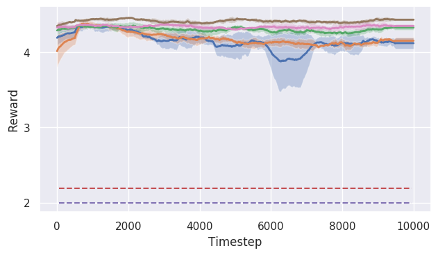
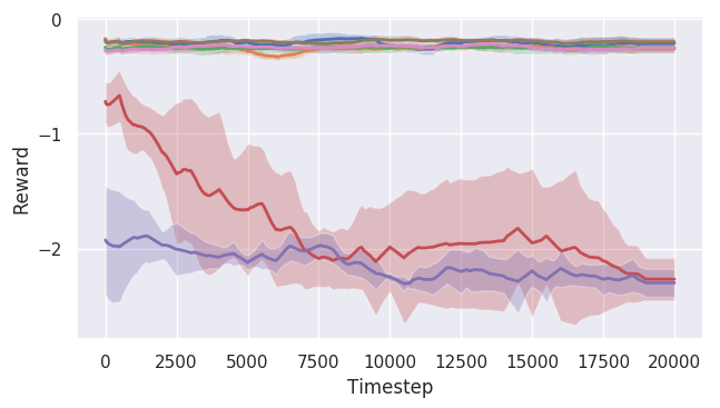
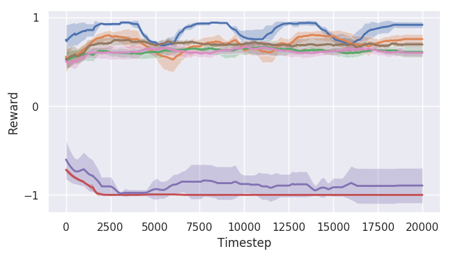
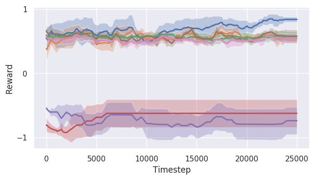
Rewards are shown in Figure 2 and Table 1, and planning is in Table 2. AOP plans only at of MPC-8, but performs comparably or better, successfully learning the desired behavior on all tasks.
Reset-Free Setting: Even with model access, these environments are challenging. In the standard episodic reinforcement learning setting, long-term action dependencies are learned from past experience over time, and this experience can be utilized when the agent resets to the initial state. However, in the online reset-free setting, these dependencies must be learned on the fly, and if the agent falls, it must return to the prior state in order to use that information, which is often harder than the original task; the model-free algorithms generally fail to overcome this challenge of long-term regret.
Vast Worlds: In the sparse mazes, MPC is significantly outperformed by AOP-TD3 (Figure 3), and the model-free algorithms struggle to make any progress at all, showing their lackluster exploration. Even POLO – the exploration mechanism of AOP – faces weaker performance, indicating that AOP-TD3 has not only correctly identified when planning is important, but is able to effectively leverage additional computation to increase its performance whilst still using less overall computation.

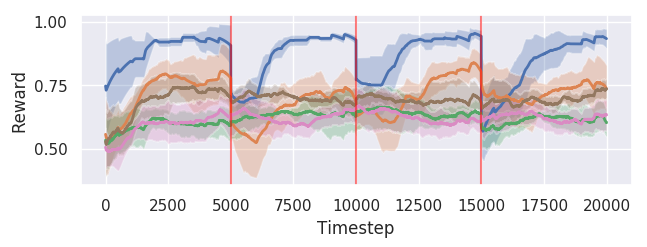
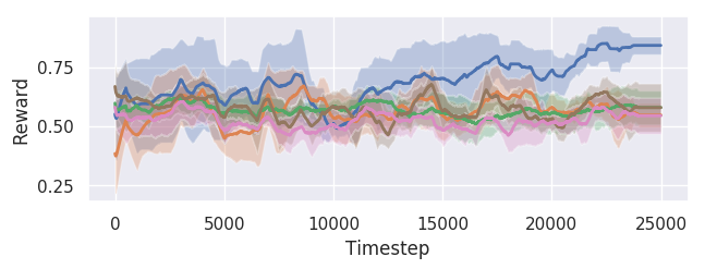
The additional performance in the sparse novel states Maze over MPC-8 also shows AOP’s ability to consolidate experience to improve performance in situations it has seen before. Furthermore, in the sparse changing worlds Maze, the performance of AOP improves over time, indicating that AOP has learned value and policy functions for effective forward transfer in a difficult exploration setting.
Policy Degradation: TD3’s performance significantly degrades in the changing worlds settings, as does PPO’s (see Figure 2). PPO, an on-policy method, struggles in general. In the novel states Hopper, where the policy is capable of directly seeing the target velocity, TD3 performs very well, even learning to outperform MPC. However, without the help of the observation, in the changing worlds, TD3’s performance quickly suffers after world changes, incurring large long-term regret. The model-based planning methods naturally do not suffer this degradation; AOP is able to maintain its performance and computational savings, even through many world changes, despite its reliance on model-free components. This phenomenon is detailed more in Appendix B.
5.4 Analysis of AOP Planning and Uncertainty Approximation
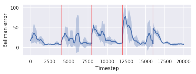
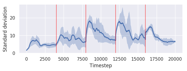
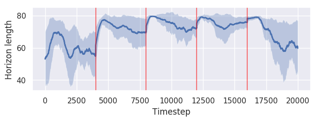
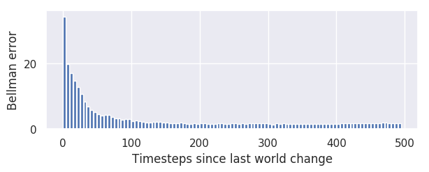
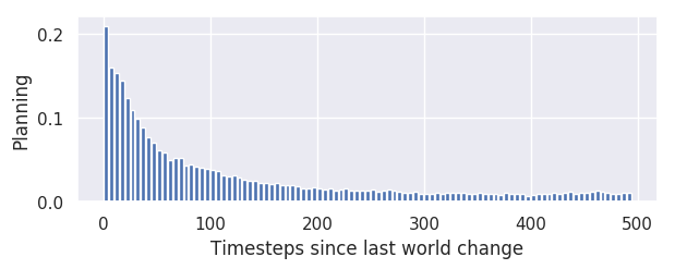
The standard deviation and Bellman error over time of AOP for the changing worlds Hopper is shown in Figure 4. After each world change, the Bellman error spikes, and then decreases as time goes on and the agent becomes more familiar with the environment. These trends are reflected in the time horizon, which decreases as the agent trains in each world, indicating that the standard deviation and Bellman error are suitable metrics for considering agent uncertainty.
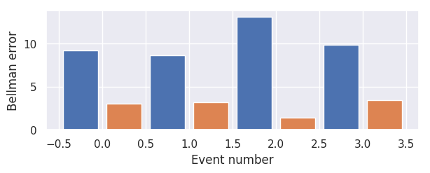
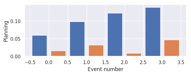
Figure 5 shows AOP behavior in the dense Mazes. When encountering novel states, Bellman error is high, but as time progresses, when confronted with the same states again, the Bellman error is low. The number of planning timesteps matches this: AOP correctly identifies a need to plan early on, but greatly saves computation later, when it is immediately able to know the correct action with almost no planning. The same effect occurs when measuring the time since the world changed for the changing worlds. At the beginning of a new world, the amount of planning is high, before quickly declining to nearly zero, almost running with the speed of a policy: faster than MPC-8.
6 Related Work
Continual learning: Most past continual learning work finn2019onlinemeta ; goodfellow2013forget ; kirkpatrick17forgetting ; parisi ; rolnick18replay ; ruvolo13ella ; schwarz18compress has focused on catastrophic forgetting, which AOP is resilient to (see Appendix B), but was not a primary focus of our work, because unlike traditional continual learning literature, the same state/input can denote different dynamics and tasks, since they are not embedded in the observation, which makes the notion of catastrophic forgetting poorly defined. In contrast, our setting emphasizes the desire to quickly perform any new task well with limited regret, which naturally includes previous tasks, but does not focus on them. In the supervised framework of vandeven19scenarios , our changing worlds setting is classified as Domain-IL, with our novel states variant being classified as the easier Task-IL. mole learns multiple models to represent different tasks for continual learning in episodic RL. In contrast to previous notions of regret alquier16regret ; besbes15stoopt ; yang16dynregret , we consider a notion of regret that focuses on how well the agent can learn in the future as a consequence of near short-term actions.
Planning and learning: Algorithms that combine planning with learning have been studied with great variety in both discrete and continuous domains exit ; pets ; polo ; poplin . Our algorithm is closest to POPLIN poplin , which uses MPC with a learned policy prior. levine2013guided ; mordatch2015interactive propose to use priors that make the planner stay close to policy outputs, which is problematic in changing worlds, when the policy is not accurate. sezener20computation proposes to use learned upper confidence bounds to evaluate the value of computation for the discrete MCTS algorithm, which is a similar notion to our work. mctsnets generalizes the MCTS algorithm and proposes to learn the algorithm instead; having the algorithm set computation levels could be interesting in our setting. azziz2018 ; pets ; mbmf ; poplin learn models of the environment to perform MPC. mbmpo ; modtrust ; metrpo utilize model ensembles to reduce model overfitting for policy learning.
7 Conclusion
We proposed AOP, incorporating model-based planning with model-free learning, and introduced environments for evaluating algorithms in a new continual lifelong learning setting. We highlighted the shortcomings of traditional RL, analyzed the performance of and signals from AOP’s model-free components, and showed experimentally that AOP was able to reduce computation while achieving high performance in difficult tasks, competitive with a significantly more powerful MPC procedure.
8 Broader Impact
Our work focuses on how we can design agents that are capable of learning in a setting where the training and evaluation environments are not distinct. Most modern applications and work in reinforcement learning (and machine learning systems more broadly) are constrained by a notion of training in a specific setting or dataset and then being applied in a real-world evaluation setting. This can be problematic in that robotic systems can encounter novel situations where the model is uncertain of how to act; this is a well-known bottleneck of deep learning applications and, for example, can be catastrophic in safety-critical scenarios, such as self-driving cars. Agents should learn to adapt gracefully to such scenarios, training while acting. Our work is a step in the direction of a setting where we have biologically-inspired, intelligent agents that can continuously learn in their lifetime in the same manner that a human learns, adapting to novel and changing situations with minimal long-term risk. However, there is still work to be done, in this setting and in reinforcement learning more broadly, to understand control in safety-critical scenarios. A potential negative impact of this work could result from abuses of RL use cases, where algorithms may be applied to situations where the decision making capability is not well understood or constrained, which could lead to user overconfidence and misuse. More intelligent agents should have strong notions of causality and hierarchy, which is currently a fundamental limitation of deep learning systems.
Acknowledgments
We would like to thank Vikash Kumar, Aravind Rajeswaran, Michael Janner, and Marvin Zhang for helpful feedback, comments, and discussions.
References
- [1] Pierre Alquier, The Tien Mai, and Massimiliano Pontil. Regret bounds for lifelong learning, 2016.
- [2] Thomas Anthony, Zheng Tian, and David Barber. Thinking fast and slow with deep learning and tree search. CoRR, abs/1705.08439, 2017.
- [3] Kamyar Azizzadenesheli, Brandon Yang, Weitang Liu, Emma Brunskill, Zachary C. Lipton, and Animashree Anandkumar. Sample-efficient deep RL with generative adversarial tree search. CoRR, abs/1806.05780, 2018.
- [4] Adrian Banks and Christopher Hope. Heuristic and analytic processes in reasoning: An event-related potential study of belief bias. Psychophysiology, 51, 03 2014.
- [5] Omar Besbes, Yonatan Gur, and Assaf Zeevi. Non-stationary stochastic optimization. Operations Research, 63(5):1227–1244, Oct 2015.
- [6] Greg Brockman, Vicki Cheung, Ludwig Pettersson, Jonas Schneider, John Schulman, Jie Tang, and Wojciech Zaremba. Openai gym. CoRR, abs/1606.01540, 2016.
- [7] Jacob Buckman, Danijar Hafner, George Tucker, Eugene Brevdo, and Honglak Lee. Sample-efficient reinforcement learning with stochastic ensemble value expansion. CoRR, abs/1807.01675, 2018.
- [8] Kurtland Chua, Roberto Calandra, Rowan McAllister, and Sergey Levine. Deep reinforcement learning in a handful of trials using probabilistic dynamics models. CoRR, abs/1805.12114, 2018.
- [9] Ignasi Clavera, Jonas Rothfuss, John Schulman, Yasuhiro Fujita, Tamim Asfour, and Pieter Abbeel. Model-based reinforcement learning via meta-policy optimization. CoRR, abs/1809.05214, 2018.
- [10] Nathaniel D Daw, Yael Niv, and Peter Dayan. Uncertainty-based competition between prefrontal and dorsolateral striatal systems for behavioral control. Nature neuroscience, 8(12):1704, 2005.
- [11] Peter Dayan and Kent C Berridge. Model-based and model-free pavlovian reward learning: Revaluation, revision, and revelation. 2014.
- [12] Chelsea Finn, Aravind Rajeswaran, Sham M. Kakade, and Sergey Levine. Online meta-learning. CoRR, abs/1902.08438, 2019.
- [13] Scott Fujimoto, David Meger, and Doina Precup. Off-policy deep reinforcement learning without exploration. CoRR, abs/1812.02900, 2018.
- [14] Scott Fujimoto, Herke van Hoof, and Dave Meger. Addressing function approximation error in actor-critic methods. CoRR, abs/1802.09477, 2018.
- [15] Ian J. Goodfellow, Mehdi Mirza, Da Xiao, Aaron Courville, and Yoshua Bengio. An empirical investigation of catastrophic forgetting in gradient-based neural networks, 2013.
- [16] Arthur Guez, Théophane Weber, Ioannis Antonoglou, Karen Simonyan, Oriol Vinyals, Daan Wierstra, Rémi Munos, and David Silver. Learning to search with mctsnets. CoRR, abs/1802.04697, 2018.
- [17] Michael Janner, Justin Fu, Marvin Zhang, and Sergey Levine. When to trust your model: Model-based policy optimization. CoRR, abs/1906.08253, 2019.
- [18] Daniel Kahneman. Maps of bounded rationality: Psychology for behavioral economics †. American Economic Review, 93:1449–1475, 02 2003.
- [19] James Kirkpatrick, Razvan Pascanu, Neil Rabinowitz, Joel Veness, Guillaume Desjardins, Andrei A. Rusu, Kieran Milan, John Quan, Tiago Ramalho, Agnieszka Grabska-Barwinska, Demis Hassabis, Claudia Clopath, Dharshan Kumaran, and Raia Hadsell. Overcoming catastrophic forgetting in neural networks. Proceedings of the National Academy of Sciences, 114(13):3521–3526, 2017.
- [20] Thanard Kurutach, Ignasi Clavera, Yan Duan, Aviv Tamar, and Pieter Abbeel. Model-ensemble trust-region policy optimization. CoRR, abs/1802.10592, 2018.
- [21] Sergey Levine and Vladlen Koltun. Guided policy search. In International Conference on Machine Learning, pages 1–9, 2013.
- [22] Kendall Lowrey, Aravind Rajeswaran, Sham M. Kakade, Emanuel Todorov, and Igor Mordatch. Plan online, learn offline: Efficient learning and exploration via model-based control. CoRR, abs/1811.01848, 2018.
- [23] John Miller. Whynot, 2020.
- [24] Volodymyr Mnih, Koray Kavukcuoglu, David Silver, Alex Graves, Ioannis Antonoglou, Daan Wierstra, and Martin A. Riedmiller. Playing atari with deep reinforcement learning. CoRR, abs/1312.5602, 2013.
- [25] Igor Mordatch, Kendall Lowrey, Galen Andrew, Zoran Popovic, and Emanuel V Todorov. Interactive control of diverse complex characters with neural networks. In Advances in Neural Information Processing Systems, pages 3132–3140, 2015.
- [26] Anusha Nagabandi, Chelsea Finn, and Sergey Levine. Deep online learning via meta-learning: Continual adaptation for model-based RL. CoRR, abs/1812.07671, 2018.
- [27] Anusha Nagabandi, Gregory Kahn, Ronald S. Fearing, and Sergey Levine. Neural network dynamics for model-based deep reinforcement learning with model-free fine-tuning. CoRR, abs/1708.02596, 2017.
- [28] Ian Osband, John Aslanides, and Albin Cassirer. Randomized prior functions for deep reinforcement learning. In S. Bengio, H. Wallach, H. Larochelle, K. Grauman, N. Cesa-Bianchi, and R. Garnett, editors, Advances in Neural Information Processing Systems 31, pages 8617–8629. Curran Associates, Inc., 2018.
- [29] Ian Osband, Charles Blundell, Alexander Pritzel, and Benjamin Van Roy. Deep exploration via bootstrapped DQN. CoRR, abs/1602.04621, 2016.
- [30] German Ignacio Parisi, Ronald Kemker, Jose L. Part, Christopher Kanan, and Stefan Wermter. Continual lifelong learning with neural networks: A review. CoRR, abs/1802.07569, 2018.
- [31] Aravind Rajeswaran, Vikash Kumar, Abhishek Gupta, Giulia Vezzani, John Schulman, Emanuel Todorov, and Sergey Levine. Learning complex dexterous manipulation with deep reinforcement learning and demonstrations. arXiv preprint arXiv:1709.10087, 2017.
- [32] Aravind Rajeswaran, Kendall Lowrey, Emanuel Todorov, and Sham M. Kakade. Towards generalization and simplicity in continuous control. CoRR, abs/1703.02660, 2017.
- [33] David Rolnick, Arun Ahuja, Jonathan Schwarz, Timothy P. Lillicrap, and Greg Wayne. Experience replay for continual learning, 2018.
- [34] Paul Ruvolo and Eric Eaton. Ella: An efficient lifelong learning algorithm. 30th International Conference on Machine Learning, ICML 2013, 28, 01 2013.
- [35] John Schulman, Filip Wolski, Prafulla Dhariwal, Alec Radford, and Oleg Klimov. Proximal policy optimization algorithms. CoRR, abs/1707.06347, 2017.
- [36] Jonathan Schwarz, Jelena Luketina, Wojciech M. Czarnecki, Agnieszka Grabska-Barwinska, Yee Whye Teh, Razvan Pascanu, and Raia Hadsell. Progress & compress: A scalable framework for continual learning, 2018.
- [37] Eren Sezener and Peter Dayan. Static and dynamic values of computation in mcts, 2020.
- [38] Gido M. van de Ven and Andreas S. Tolias. Three scenarios for continual learning. CoRR, abs/1904.07734, 2019.
- [39] Tingwu Wang and Jimmy Ba. Exploring model-based planning with policy networks. CoRR, abs/1906.08649, 2019.
- [40] Grady Williams, Andrew Aldrich, and Evangelos A. Theodorou. Model predictive path integral control using covariance variable importance sampling. CoRR, abs/1509.01149, 2015.
- [41] Tianbao Yang, Lijun Zhang, Rong Jin, and Jinfeng Yi. Tracking slowly moving clairvoyant: Optimal dynamic regret of online learning with true and noisy gradient, 2016.
- [42] Yuke Zhu, Ziyu Wang, Josh Merel, Andrei Rusu, Tom Erez, Serkan Cabi, Saran Tunyasuvunakool, János Kramár, Raia Hadsell, Nando de Freitas, et al. Reinforcement and imitation learning for diverse visuomotor skills. arXiv preprint arXiv:1802.09564, 2018.
test
Appendix
Appendix A Further Discussion of Long-Term Regret
In this section, we provide more details, commentary, and the proof for the analysis from Section 4.1.
A.1 Definitions
Recall that we define the regret as the suboptimality of the MPC planner when using an -step horizon against an optimal infinite-horizon MPC policy, where actions for timesteps after time are given by the agent policy , representing the agent’s ability to replan later and decide on those actions. Note that this is not the learned parameterized policy, but representing the agent as a whole.
Specifically, when the dynamics are deterministic (simplifying the equations), as in this work, the MPC policy is optimized as the following objective over the ground-truth model:
| (2) |
In pure MPC, , which is problematic when is much smaller than the lifetime horizon. For our algorithms, we use a learned terminal value function parameterized as a neural network. In shooting-based MPC, as used in this work, the MPC policy simply takes the form of open-loop actions, although the result holds for more general forms of closed-loop optimization.
Our formulation of regret (from Definition 4.1) yields the following decomposition:
| (3) |
where the long-term and short-term regret are defined as:
| (4) |
| (5) |
Note that the short-term regret is not necessarily positive, and likely is negative from a practical perspective, as MPC will prefer to greedily optimize for return in the first steps, particularly when inaccurately models the true value of the future states.
A.2 Effect of Planning Horizon on Long-Term Regret
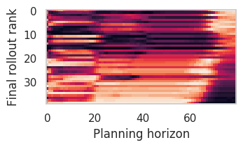
In Figure A.1, we show the evaluation of each trajectory in the sampled population of an MPC iteration. Each row represents a trajectory, and are ordered vertically in terms of the strongest trajectory at the top, and the weakest at the bottom, where we run a more extended simulation to approximate the total return for the trajectories. Each column represents a timestep of planning, e.g. the left of the figure shows short-horizon planning and the right shows long-horizon planning. The pixel at cell (row , column ) represents the ranking of trajectory when evaluated by MPC with a horizon of ; white denotes the strongest rankings, and purple/black denote the weakest rankings. An ideal MPC with an accurate value approximator is able to order the trajectories perfectly, which is approximately done when planning with the long horizon () on the far right.
Figure A.1 indicates the issue with only short-term planning, and a key reason why reset-free environments (particularly in environments with momentum or short-term rewards like Hopper) are difficult. In the presence of a weak (or absent) value function approximator, incorrect assignment of values to trajectories can help lead to catastrophic mistakes.
A.3 Proof of Lemma 1
Let denote the optimal trajectory generated by -horizon planning and denote the trajectory generated by -horizon planning.
Because the optimum of the -horizon planner is realized with , the planner evaluation incorrectly assigns . Substituting for the individual terms, this yields:
Rearranging and bounding as the maximum difference in the sum of rewards:
Now, we can use this result and substitute the assumed bounds to derive the result:
A.4 Remarks on Lemma 1
We note the following characteristics of the above three inequalities:
-
1.
The first inequality, bounding long-term policy suboptimality, follows from the agent being unable to execute an optimally, and is greatest when the agent is unable to progress through learning at all. More powerful procedures (like MPC) are less subject to this, and this is amplified when “pseudo-terminal” states are present in the MDP.
-
2.
The second inequality, bounding the value function approximator, follows from overestimation of the desired state and underestimation of the optimal state.
-
3.
The third inequality, bounding the short-term greedy optimization, is tightest when the MDP allows for high short-term gain in exchange for longer-term penalty, like the Hopper environment, and the MPC planning procedure optimally solves for the maximum, and is weaker when the planning procedure is softer (ex. using a procedure like MPPI), or starts with a long-term prior (like a policy) and then performs regularized local optimization.
Appendix B Episodic Policy Performance and Policy Degradation
Here we expand on our consideration of policy degradation from Section 5.3. In Figure B.1, we plot an episodic reward of the policy running from the initial starting state after each timestep (for the current target velocity), which can be considered to be the standard reinforcement learning setting with a different training regimen. Note that since the AOP policy is learned from off-policy data (the planner), it suffers from divergence issues and should be weaker than TD3 on its own [13].
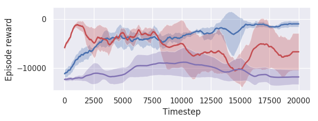
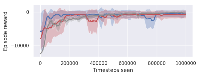
Matching the result in Figure 2 (a), the TD3 (red) policy degrades in performance over time, but the AOP (blue) policy does not, despite TD3 learning much faster initially. Because the optimization procedure is the same, this result suggests that the policy degradation effect likely stems from exploration, rather than from an issue with optimization or the network falling into a parameter “trap”.
Figure B.1 shows the result of tuning the policy learned by AOP after seeing every target velocity once (blue) vs. by TD3 (red) vs. training a new policy from scratch (gray), learning via the standard episodic TD3 algorithm on the first target velocity. The AOP policy learns faster, showing that it is capable of quick backward transfer and adaptation, while TD3 by itself is comparable to starting over.
Appendix C Additional Algorithm Specification
Appendix D Hyperparameters
Our hyperparameters are chosen coarsely from similar work, and new hyperparameters were approximately chosen based on performance in the 2D maze environment. We found most of the hyperparameters to not be very sensitive, except for the MPPI temperature, which is important for all algorithms and not specific to AOP.
D.1 Adaptive Online Planning Hyperparameters
For AOP, we set , and . For the first planning iteration we set , and for the later planning iterations, , which helps to prioritize the use of the planner. These values were coarsely chosen by looking at general values of the value function, and we did not tune these hyperparameters much. We found that the algorithm is not overly sensitive to the thresholds in dense reward environments, which we also show in Appendix D.1.1. The only exception to this is that we set for the Humanoid environment, as the value function is harder to learn accurately. In the sparse reward settings, we set , in order to avoid early termination of exploration (we do not change the hyperparameters determining the number of planning iterations). This is a natural concession that is hard to resolve in the reset-free setting as the exploration in the problem is not as well-defined, and must be addressed by some broader change to the setting, which we leave for future work.
D.1.1 Sensitivity to Thresholds
To test the sensitivity of AOP to the heuristic thresholds from Section 4.2, we run a rough grid search with wider values for and in the Hopper changing worlds environment. The average reward for each setting is shown in Table D.1 and learning curves are shown in Figure D.1. AOP is somewhat more sensitive to the setting of early on in training, as a higher value corresponds to less planning, but this effect quickly dissipates. As a result, while the choice of and is somewhat arbitrary, we do not believe that AOP is particularly sensitive to them.
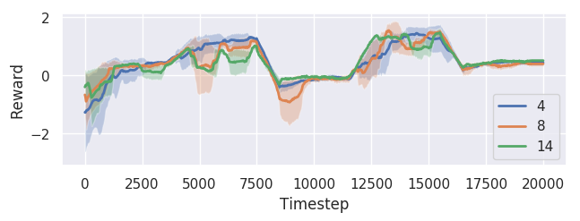
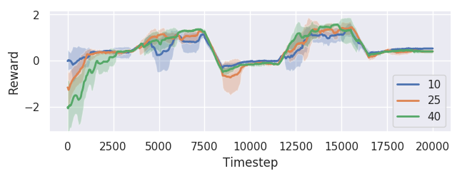
| Standard Deviation : | 4 | 8 (Default) | 14 |
|---|---|---|---|
| Average reward | 0.47 0.20 | 0.42 0.05 | 0.44 0.16 |
| Bellman Error : | 10 | 25 (Default) | 40 |
| Average reward | 0.47 0.17 | 0.47 0.09 | 0.43 0.24 |
D.1.2 Uncertainty Heuristics in the WhyNot Environment
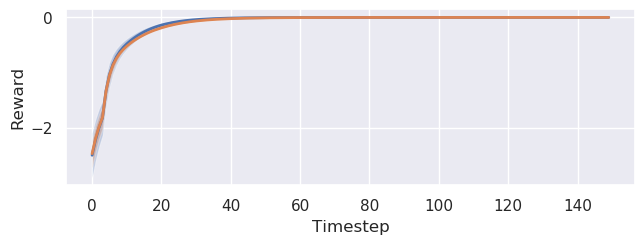
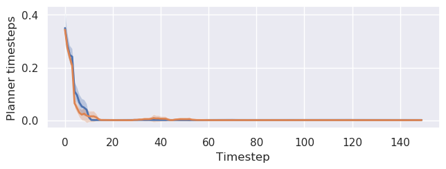
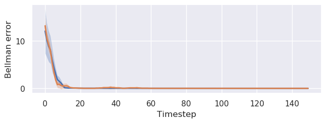
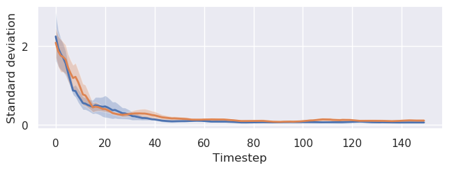
To consider whether the heuristics generalize outside of our physics-based settings, we also test AOP in the causal WhyNot simulator [23] on its continuous control Zika task. Using the same hyperparameters, AOP achieves optimal performance ( MPC), shown in Table D.2. The agent correctly plans less once converged, reflected in the uncertainty metrics, shown in Figure D.2.
| Algorithm: | AOP-TD3 | AOP-BC | MPC-3 |
|---|---|---|---|
| Average reward | -0.12 0.05 | -0.13 0.02 | -0.14 0.01 |
D.2 Model Predictive Control Hyperparameters
Our MPPI temperature is set to 0.01. The other planning hyperparameters are shown below. See Section 3.3 for interpretation of policy optimization as a special case of AOP. Surprisingly, we found TD3 to perform worse with more than 1 trajectory per iteration.
| Parameter | AOP-TD3/AOP-BC | POLO | TD3 | PPO | MPC |
|---|---|---|---|---|---|
| Planning horizon | 1-80 | 80 | 256 | 128 | 80 |
| Planning iterations per timestep | 0-8 | 3 | 1 | 1 | 3, 8 |
| Trajectories per iteration | 40 | 40 | 1 | 32 | 40 |
| Noise standard deviation | 0.1 | 0.1 | 0.2 | - | 0.1 |
For the Humanoid environment only, all the MPC-based algorithms use 120 trajectories per iteration and a noise standard deviation of .
D.3 Network Architectures
For our value ensembles, we use an ensemble size of and . The value functions are updated in batches of size for gradient steps every timesteps. All networks use tanh activations and a learning rate of , trained using Adam. Network sizes are shown below.
| Environment | AOP-TD3/AOP-BC | POLO | TD3 | PPO |
|---|---|---|---|---|
| Hopper | ||||
| Humanoid | ||||
| Ant | ||||
| Maze |
D.4 Policy Optimization Hyperparameters
Our TD3 uses the same hyperparameters as the original authors [14], where for every timestep, we run a rollout of length 256 and run 256 gradient steps. In the TD3 used for the episodic policy learning experiment in Section B, we run rollouts of length 1000 and run 1000 gradient steps after each rollout, equivalent to the standard TD3 setting with no terminal states.
Our PPO uses , , batch sizes of , and gradient steps per iteration, which we found to yield the best results out of a set of common hyperparameters. For behavior cloning, we run gradient steps on batches of size every timesteps. For the policy in AOP-TD3, we run gradient steps on batches of size every timesteps.
Appendix E Environment Details
E.1 Environment Descriptions
Hopper: We use the Hopper agent from OpenAI Gym [6]. The agent is tasked with achieving a target forward -velocity (in the range of ) in the following settings:
-
•
Standard (S): the target velocity is constant
-
•
Novel states (NS): the target velocity changes, but is observed by the state
-
•
Changing worlds (CW): the target velocity changes and is not observed by the state
Humanoid: We use the SlimHumanoid agent from OpenAI Gym [6], which reduces the dimension of the state space significantly. The agent is tasked with achieving a target forward -velocity while the mass of its right arm varies (in the range of ):
-
•
Standard (S): the head mass is constant
-
•
Changing worlds (CW): the head mass varies and is not observed by the state
Ant: We use the Ant agent from OpenAI Gym [6], with the full state space. The agent is tasked with achieving a target forward -velocity while a joint at random is disabled (e.g. the action is set to ):
-
•
Standard (S): no joints are disabled
-
•
Changing worlds (CW): the disabled joint varies and is not observed by the state
Maze: We use a 2D particle maze environment. The walls of the maze change and the goal swaps between two locations to avoid the agent staying still at the goal forever. The goal is always observed, making the observation space 4D. We test on both dense and sparse reward variants.
-
•
Novel states (NS): the walls are constant, but the new unseen goals appear periodically
-
•
Changing worlds (CW): the goals stay in the same two places, but the walls change
E.2 Reward Specifications
In the online setting, the agent receives no signal from termination states, i.e. it becomes more difficult to know not to fall down in the cases of Hopper and Ant. This leads to a “rolling” behavior for the Hopper and a “wiggling” behavior for the Ant, which, while these modes can capable of achieving the same velocities, are not particularly meaningful or difficult to achieve. To amend this, and achieve the same stable/interpretable behavior as the standard reinforcement learning setting, we set the reward functions as the following for our environments, in the style of [22, 32]:
| Environment | Reward Function |
|---|---|
| Hopper | |
| Humanoid | |
| Ant | |
| Maze (Dense) | |
| Maze (Sparse) |
Appendix F Detailed Experimental Graphs
Additional graphs are provided for the fraction of planning timesteps vs MPC-8 and reward curves for all environments in Figures F.1 and F.2, respectively.

(a) Standard Hopper
(b) Novel states Hopper
(c) Changing worlds Hopper
(d) Standard Humanoid
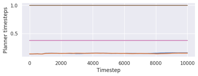
(e) Changing worlds Humanoid
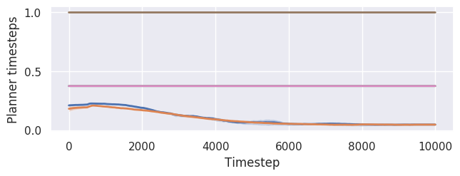
(f) Standard Ant
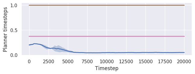
(g) Changing worlds Ant
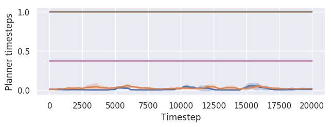
(h) Novel states Maze (D)
(i) Changing worlds Maze (D)
(j) Novel states Maze (S)
(k) Changing worlds Maze (S)

(a) Standard Hopper
(b) Novel states Hopper

(c) Changing worlds Hopper
(d) Standard Humanoid

(e) Changing worlds Humanoid
(f) Standard Ant

(g) Changing worlds Ant
(h) Novel states Maze (D)

(i) Changing worlds Maze (D)
(j) Novel states Maze (S)
(k) Changing worlds Maze (S)