Analysis of the H.E.S.S. public data release with ctools

The ctools open-source software package was developed for the scientific analysis of astronomical data from Imaging Air Cherenkov Telescopes (IACTs), such as H.E.S.S., VERITAS, MAGIC, and the future Cherenkov Telescope Array (CTA). To date, the software has been mainly tested using simulated CTA data; however, upon the public release of a small set of H.E.S.S. observations of the Crab nebula, MSH 15–52, RX J1713.7–3946, and PKS 2155–304 validation using real data is now possible. We analysed the data of the H.E.S.S. public data release using ctools version 1.6 and compared our results to those published by the H.E.S.S. Collaboration for the respective sources. We developed a parametric background model that satisfactorily describes the expected background rate as a function of reconstructed energy and direction for each observation. We used that model, and tested all analysis methods that are supported by ctools, including novel unbinned and joint or stacked binned analyses of the measured event energies and reconstructed directions, and classical On-Off analysis methods that are comparable to those used by the H.E.S.S. Collaboration. For all analysis methods, we found a good agreement between the ctools results and the H.E.S.S. Collaboration publications considering that they are not always directly comparable due to differences in the datatsets and event processing software. We also performed a joint analysis of H.E.S.S. and Fermi-LAT data of the Crab nebula, illustrating the multi-wavelength capacity of ctools. The joint Crab nebula spectrum is compatible with published literature values within the systematic uncertainties. We conclude that the ctools software is mature for the analysis of data from existing IACTs, as well as from the upcoming CTA.

1 Introduction

Gamma-ray photons are powerful probes for the most extreme and violent phenomena in the Universe. Advancements made in the past two decades to the observation of very-high-energy (VHE) gamma rays ($\ga 100$ GeV) that use ground-based Imaging Air Cherenkov Telescopes (IACTs) have revealed an unexpected ubiquity of sources that attest to the acceleration of particles to relativistic energies (e.g. Holder 2012). Studying these VHE gamma rays provides unique insights into the acceleration physics, the nature of the accelerated particles, relativistic particle propagation, the impact of the particles on the source environment, and the distribution of particle accelerators in the Universe. VHE gamma rays also probe the intergalactic medium and allow for the assessment of its content in infrared radiation and magnetic fields. In addition, VHE gamma rays have the potential to probe the particle nature of dark matter and physics beyond the standard model (CTA Consortium 2019).

Making observations of VHE gamma rays using IACTs is complicated by the presence of a large background due to cosmic-ray induced air showers that are difficult or sometimes impossible to distinguish from the air showers generated by gamma rays. In classical IACT data analyses, the residual background is taken into account by estimating its contribution from gamma-ray source free regions in the same field of view, or, more rarely, from independent ‘Off’ observations. Several techniques for background estimation exist and depending on the analysis aims, different methods are advocated (e.g. Berge et al. 2007). Limiting factors are that the methods generally rely on assumed symmetries of the background rates in the field of view that are not necessarily verified, and that they generally require large enough source-free regions for the background estimation in the same field of view. Also, the handling of complex source morphologies and confused or overlapping sources is not always straightforward (e.g. H.E.S.S. Collaboration et al. 2018).

We propose an alternative data analysis approach that relies on a parametrised joint modelling of the spatial and spectral event distributions, comprising model components for gamma-ray sources and background. The model is adjusted to the data by using a fitting algorithm, and estimates for all free model parameters are obtained by maximising the likelihood function, given the model and the data. Source confusion, as well as complex source morphologies, can be consistently treated with this method, and uncertainties in the residual background can be treated as nuisance parameters, reducing the systematic uncertainties in the analysis. The challenge, however, is to devise a parametrised model that describes the residual background with sufficient accuracy to allow for a reliable determination of gamma-ray source characteristics.

We implemented these analysis methods in ctools, an open-source software package developed in the context of the Cherenkov Telescope Array (CTA) project (Knödlseder et al. 2016a, b). The ctools are inspired by science analysis software available for existing high-energy astronomy instruments, and they follow the modular ftools model developed by the High Energy Astrophysics Science Archive Research Center. The latest release of this software can be downloaded from http://cta.irap.omp.eu/ctools/ which also provides user documentation and analysis tutorials. In this paper we use the ctools release version 1.6. The software has been extensively used on simulated CTA data (Hütten et al. 2016; Petropoulou et al. 2017; Acero et al. 2017; De Franco et al. 2017; Burtovoi et al. 2017; Balázs et al. 2017; Patricelli et al. 2018; Hütten & Maier 2018; Romano et al. 2018; Landoni et al. 2019; Tavecchio et al. 2019; Yang & Razzaque 2019; CTA Consortium 2019) but so far had not yet been validated on existing IACT data. Moreover, no systematic comparison between the classical and multi-component likelihood fitting methods was performed on an existing IACT data set. Upon the recent release of a small dataset obtained by the H.E.S.S. telescopes into the public domain (H.E.S.S. Collaboration 2018), we can now address these issues. This validation is an important milestone in the qualification of ctools for the upcoming CTA. It also paves the way towards broader usage of ctools for the analysis of current IACT data.

2 Data analysis

2.1 Public data release

The H.E.S.S. public data release includes 48.6 hours of observing time, and comprises observations of the Crab nebula, MSH 15–52, RX J1713.7–3946, PKS 2155–304, and empty-field regions performed with the H.E.S.S. I array (H.E.S.S. Collaboration 2018). The data are typically divided into 28-minute-long observations during which the telescopes track a position in the sky. In total, 105 such observations are included in the data release. Each observation comprises an event list and corresponding instrument response information, it also uses the ‘Heidelberg calibration’ and a Hillas event reconstruction, and applies standard cuts and a spectral data quality selection (see Aharonian et al. 2006a and H.E.S.S. Collaboration 2018 for details). The data are provided in FITS format. Table 1 summarises the key parameters of the datasets that are analysed in this paper.

Table 1: Key parameters of datasets analysed in this paper. $N_{\rm obs}$ is the number of observations, $T_{\rm obs}$ is the exposure time in hours, $T_{\rm live}$ is the live time in hours, and $E_{\rm thres}$ is the minimum safe energy threshold.

Source name	$N_{\rm obs}$	$T_{\rm obs}$	$T_{\rm live}$	$E_{\rm thres}$
		h	h	GeV
Crab nebula	4	1.87	1.75	661
MSH 15–52	20	9.13	8.33	380
RX J1713.7–3946	15	7.01	6.29	201
PKS 2155–304 (flare)	15	7.04	6.58	251
PKS 2155–304 (steady)	6	2.81	2.61	251
Empty fields	45	20.69	19.23	251

2.2 Data preparation

We prepared and analysed the data using a set of Python scripts that we released on GitHub. After downloading the H.E.S.S. data we generated for each target an observation definition file that collects all observations and the associated instrument response information in a single file. These observation definition files are available for download. For each target we then run the ctselect tool on each of the files, and select all events within $2^{\circ}$ of the pointing direction with reconstructed energies above the safe energy threshold, which is the energy at which the energy bias equals 10%, at an offset of $1^{\circ}$ in the field of view (H.E.S.S. Collaboration 2018). The values of the safe energy thresholds are stored in the effective area component of the instrument response function of each observation, and limiting the analysis to energies above this threshold ensured that we used only events for which the instrument response information is accurate.

2.3 Empty-field observations and background model

We used the 45 empty-field observations that are included in the H.E.S.S. public data release to develop a parametric model that is suitable to describe the spatial and spectral distribution of the H.E.S.S. background events in the H.E.S.S. public data release. We used the factorisation

$$B(\@vec{p}^{\prime},E^{\prime})=B_{\mathrm{spatial}}(\@vec{p}^{\prime}|E^{\prime})\times B_{\mathrm{spectral}}(E^{\prime})$$ (1)

to model the background event distribution, where $\@vec{p}^{\prime}$ is the reconstructed event direction in the field of view and $E^{\prime}$ is the reconstructed event energy. The first term represents the energy-dependent spatial component of the background model, while the second term represents the field-of-view-averaged background spectrum.

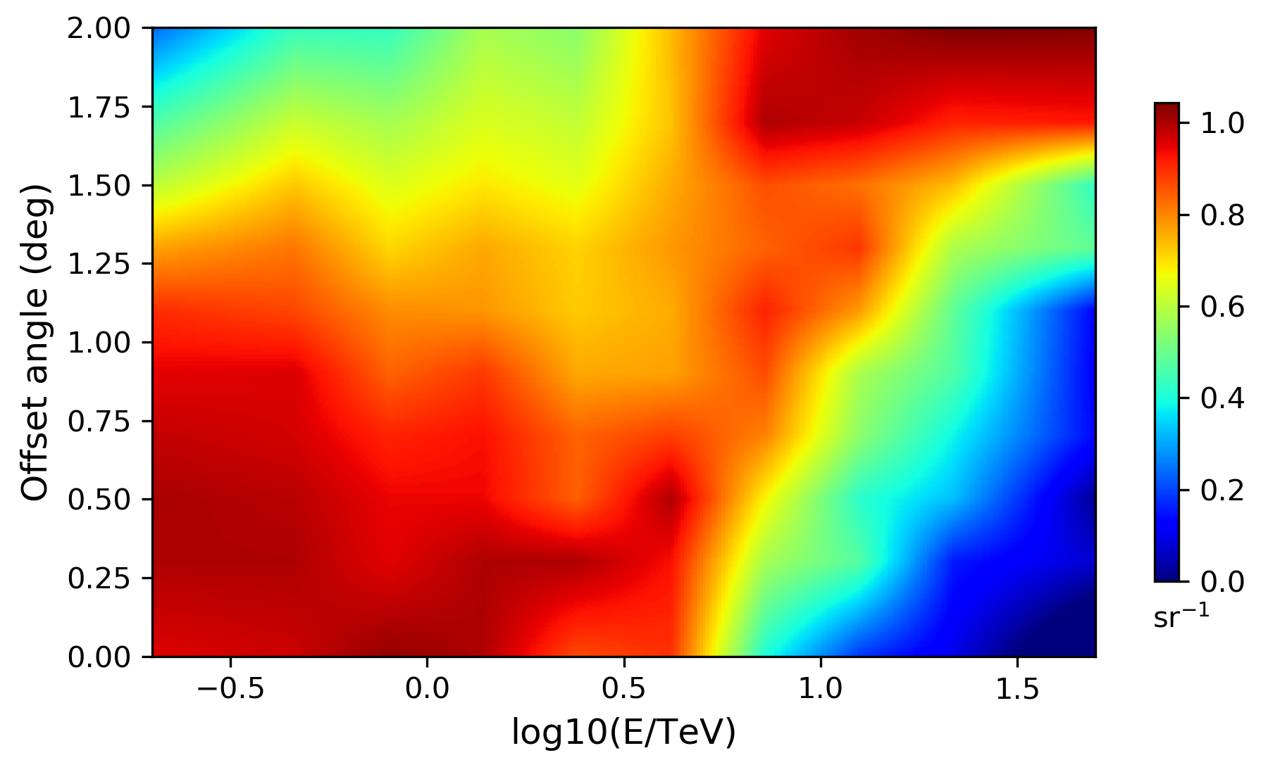
Since the spatial distribution of background events in the H.E.S.S. data depends in a rather complex way on event energy (Berge et al. 2007), we derive the spatial component from a two-dimensional lookup table $B_{\mathrm{lookup}}(\theta,E^{\prime})$ that gives the background rate per unit solid angle as a function of offset angle $\theta$ from the pointing direction and event energy $E^{\prime}$. We generated this lookup table by filling the events from the 45 empty-field observations into a histogram spanned by ten $\theta$ bins of equal size and ten logarithmically-spaced energy bins, and dividing the content of each bin by the solid angle of the corresponding $\theta$ interval. The background spatial distribution is known to depend on the zenith angle of the observations (Berge et al. 2007). However, with the limited statistics of the 45 empty-field observations of the public dataset we do not find significant variations in the background rate as a function of $\theta$ for different zenith angles within the relevant energy range of the analysis. Therefore, we neglect effects related to the zenith angle in the generation of the lookup table. This aspect should be further investigated by using larger datasets. The lookup table covers a $\theta$ range of $0^{\circ}$ to $2^{\circ}$ and an energy range of $0.2$ TeV to $50$ TeV. For each energy bin of the lookup table, all histogram values were divided by the maximum histogram value of the energy bin, so that the maximum background rate value for a given energy bin is 1. Figure 1 shows the resulting lookup table that we used throughout this paper. To evaluate $B_{\mathrm{lookup}}(\theta,E^{\prime})$ at a specific pair of $\theta$ and $E^{\prime}$ values, the lookup table is bi-linearly interpolated in offset angle and the logarithm of energy.

The lookup table provides background rates that are azimuthally symmetric with respect to the pointing direction. Some observations, however, have non-negligible gradients in the background-event distribution over the field of view. Hence we multiply the lookup table by the function

$$B_{\mathrm{gradient}}(\@vec{p}^{\prime})=1+G_{\mathrm{x}}x+G_{\mathrm{y}}y,$$ (2)

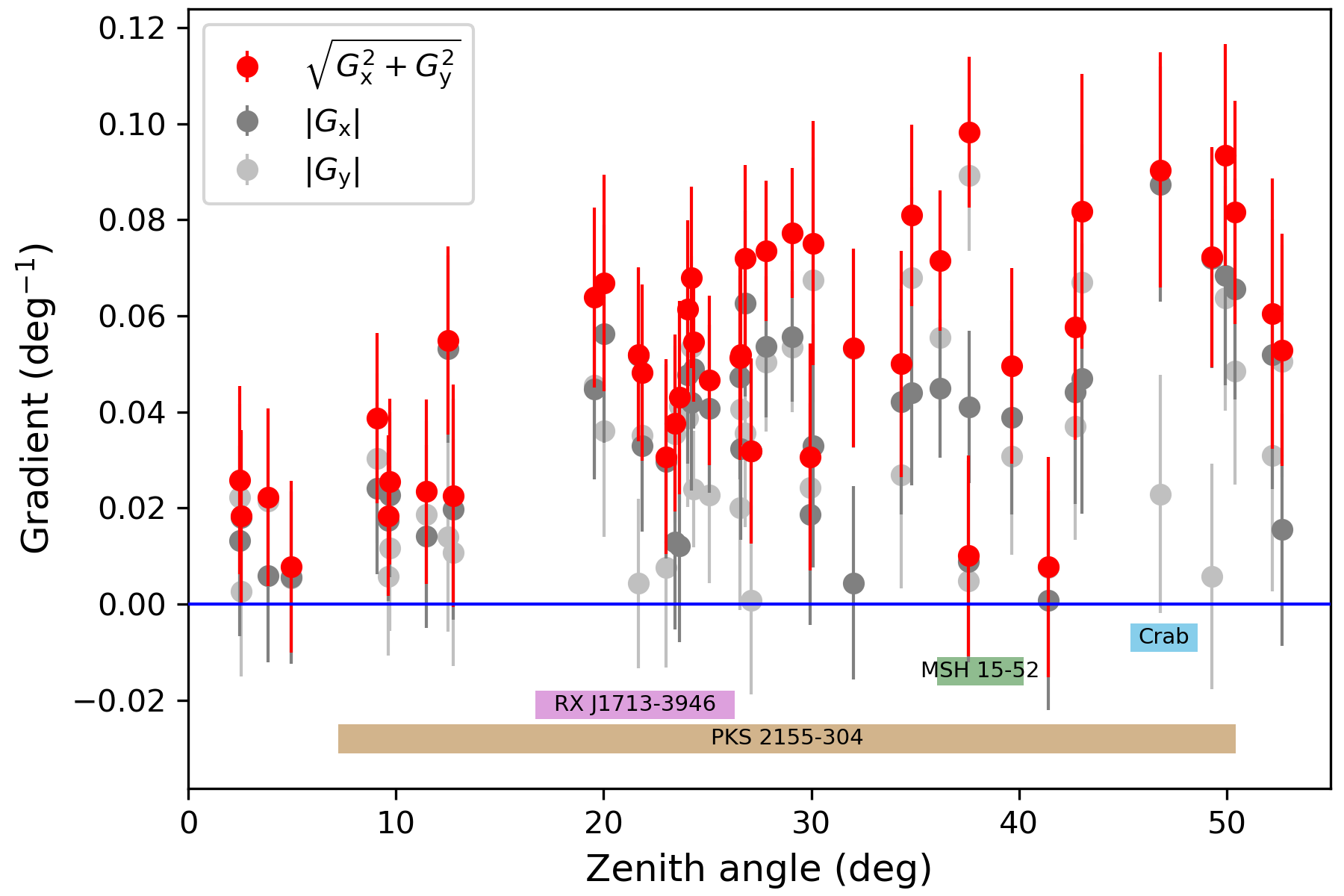
where $G_{\mathrm{x}}$ and $G_{\mathrm{y}}$ are the gradients in the $x$ and $y$ direction, and $x=\theta\cos\phi$ and $y=\theta\sin\phi$ are the nominal field-of-view coordinates, with $\phi$ being the azimuth angle around the pointing direction $x=y=0$. Figure 2 shows the fitted $G_{\mathrm{x}}$ and $G_{\mathrm{y}}$ parameters, as well as the total gradient $(G_{\mathrm{x}}^{2}+G_{\mathrm{y}}^{2})^{1/2}$, as a function of zenith angle for the 45 empty-field observations. It illustrates that this correction is indeed required by the data. Specifically, spatial gradients become more important for larger observation zenith angles, which is expected to some extent since for larger zenith angles the atmospheric depth variation over the field of view becomes larger. For information we indicate also as horizontal bars the zenith angle ranges corresponding to observations of the four sources that are included in the H.E.S.S. public data release. No obvious trends are seen for the spatial gradients as a function of azimuth angle. To summarise, the energy-dependent spatial distribution of the background is described by

$$B_{\mathrm{spatial}}(\@vec{p}^{\prime}|E^{\prime})=B_{\mathrm{lookup}}(\theta,E^{\prime})\times B_{\mathrm{gradient}}(\@vec{p}^{\prime}),$$ (3)

with two parameters $G_{\mathrm{x}}$ and $G_{\mathrm{y}}$ adjusted for each observation.

Figure 1: Background lookup table derived from all 45 empty-field observations. The table was interpolated bi-linearly to visualise the function $B_{\mathrm{lookup}}(\theta,E^{\prime})$ that was used for background modelling.

The spectral distribution of the background events varies substantially between observations, and we therefore adopted a piece-wise broken power law

$$B_{\mathrm{spectral}}(E^{\prime})=B_{i}\left(\frac{E^{\prime}}{E^{\prime}_{i}}\right)^{-\Gamma_{i}}\,\,\mathrm{for}\,\,E^{\prime}_{i}\leq E^{\prime}<E^{\prime}_{i+1},$$ (4)

with $\Gamma_{i}=-\ln{(B_{i}/B_{i+1})}/\ln{(E^{\prime}_{i}/E^{\prime}_{i+1})}$ to accommodate this diversity. The $B_{i}$ are the background rates at the node energies $E^{\prime}_{i}$ which are determined by model fitting. We found that eight logarithmically-spaced energy nodes between the minimum and maximum energy of the analysis interval provide a satisfactory description of the energy dependence of the background rates of the H.E.S.S. observations (e.g. left panel of Fig. 3). $B_{\mathrm{spectral}}(E^{\prime})$ is hence described by the eight parameters $B_{0}$ to $B_{7}$, and in total, our background model $B(\@vec{p}^{\prime},E^{\prime})$ has ten free parameters for each observation.

Figure 2: Fitted spatial background gradients as a function of zenith angle for the empty-field observations. The red points show the total gradient $(G_{\mathrm{x}}^{2}+G_{\mathrm{y}}^{2})^{1/2}$, the grey points show the absolute values of the gradients $G_{\mathrm{x}}$ and $G_{\mathrm{y}}$. The horizontal bars indicate the intervals of zenith angle covered by the source observations.

Figure 3: Stacked residuals of all 45 empty-field observations after fitting the csbkgmodel background model to each individual observation. The left panel shows the residual count spectrum after summing over the entire field of view. The centre panel shows the histogram of significances, determined after summing over energy and by sampling the events into bins of $0.2^{\circ}\times 0.2^{\circ}$. The right panel shows a residual map in the field-of-view coordinate system. The residual map is summed over all energies and was computed for a correlation radius of $0.2^{\circ}$. Residuals are shown in units of significance expressed in Gaussian $\sigma$ and are computed using Equations 9 and 10.

Figure 4: Counts spectra and residuals for nine spatial sub-regions of the field of view for all 45 empty-field observations stacked in the field-of-view coordinate system. The location of each sub-region in the field of view is indicated by the red box in the $3\times 3$ grid that is displayed in each panel.

Figure 5: Radial counts profiles and residuals as a function of offset angle $\theta$ for six energy bands between $0.2$ and $20$ TeV for all 45 empty-field observations stacked in the field-of-view coordinate system. The error bars on the counts are computed using the square root of the counts.

To ensure the convergence of the maximum likelihood fitting algorithm for this specific background model, initial values need to be determined for all ten parameters that are reasonably close to their final values. The tricky part is the determination of initial values for the background rates $B_{i}$ since they vary by more than two orders of magnitude between the lowest and highest energies, and their values differ significantly between observations. We found that the following two-step process provides robust results for each individual observation. In a first step, a simplified background model is fitted to the data using a maximum likelihood algorithm, where $B_{\mathrm{spectral}}(E^{\prime})$ is assumed to follow a simple power law, reducing the number of free spectral parameters from eight to two. The resulting power law is then evaluated at each node energy to determine a first guess of the values of $B_{i}$. In a second step, the full background model is then fitted to the data to refine the $B_{i}$ values. The resulting ten parameter values are then stored as the initial values of the background model parameters.

We implemented the algorithm that prepares this and other background models for each individual observation in the csbkgmodel script. The script, provided a lookup table for the spatial component, performs all necessary steps and produces a model definition file that can be used as background model for the analysis of the H.E.S.S. data.

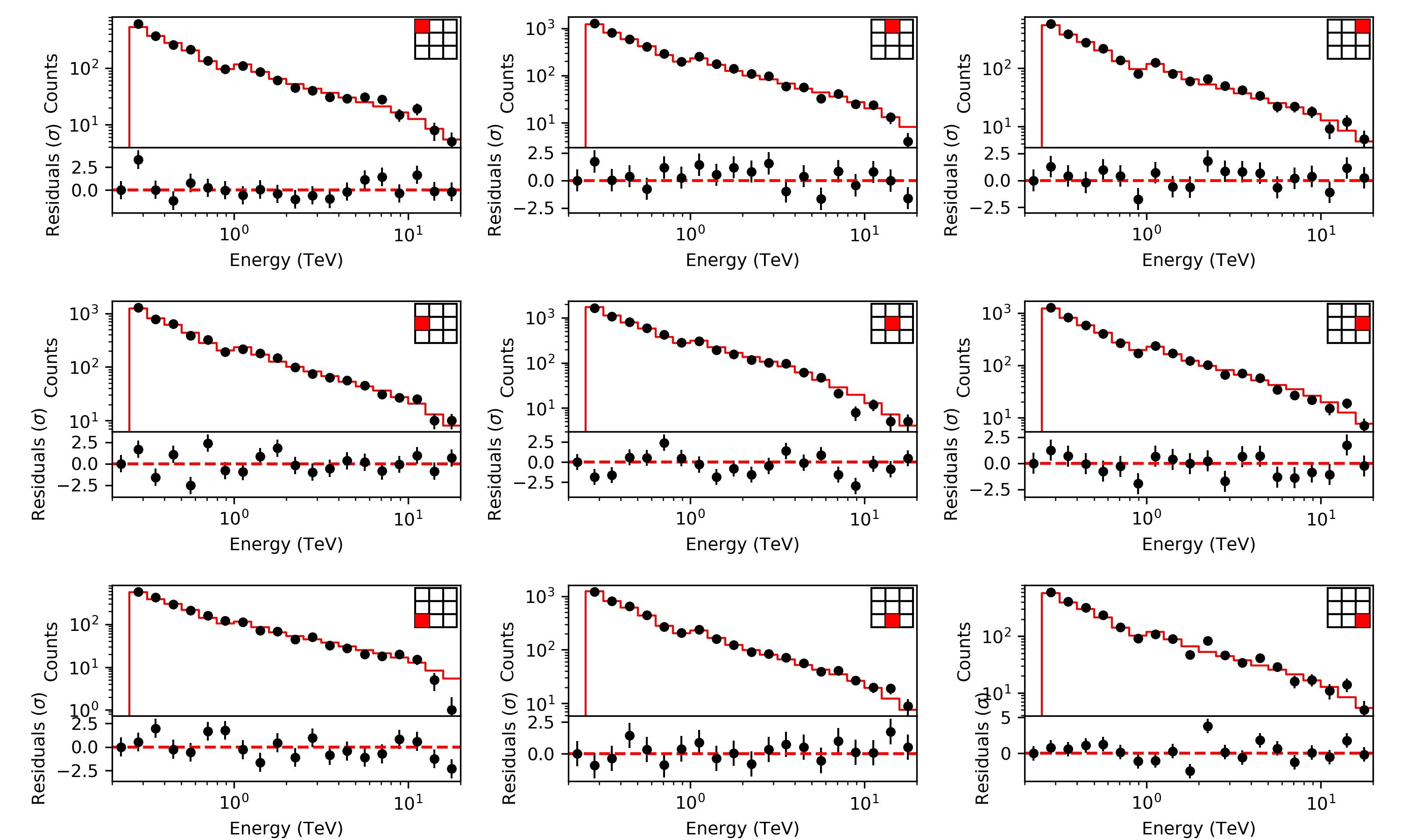
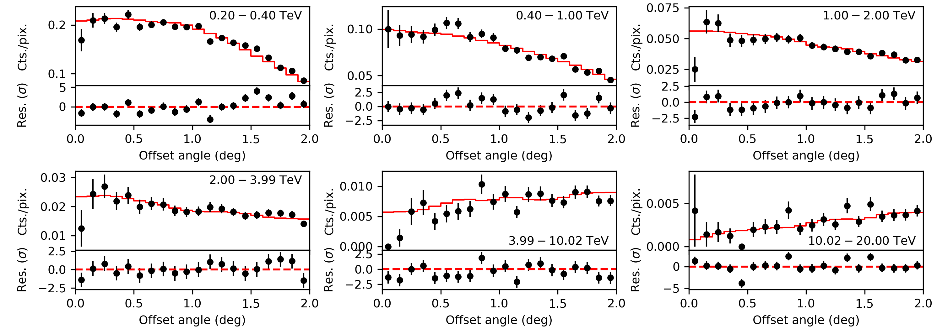
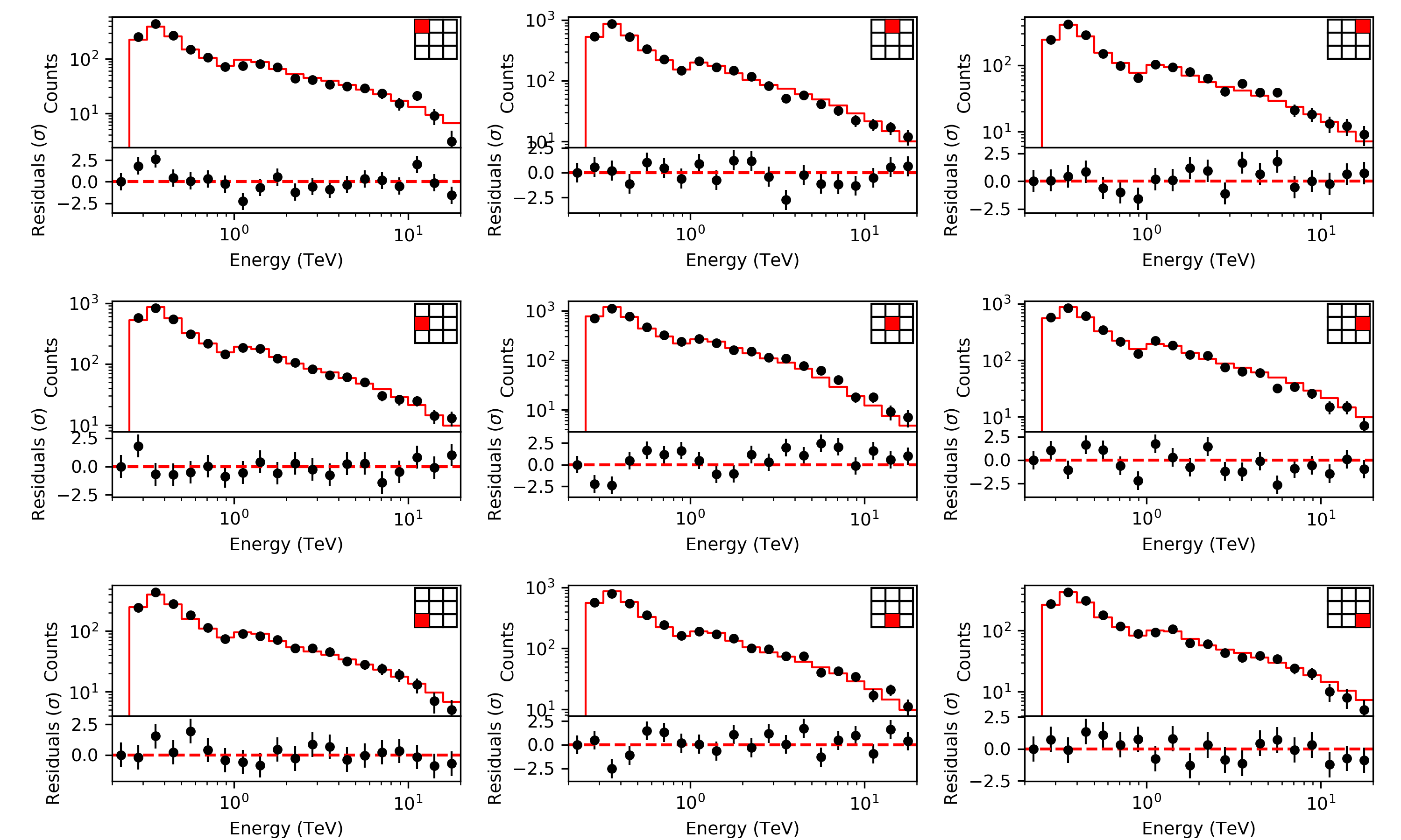
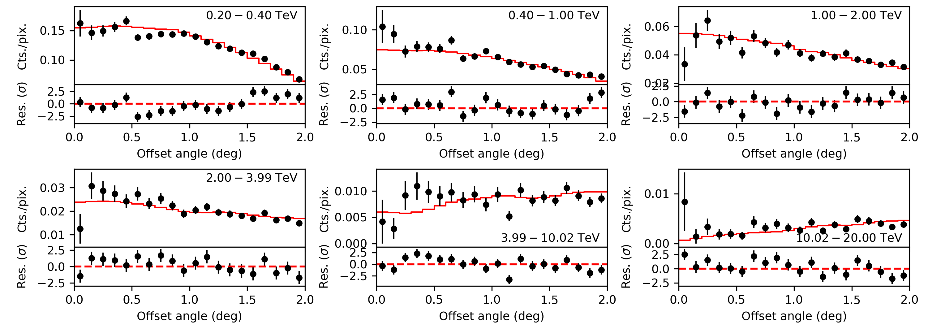
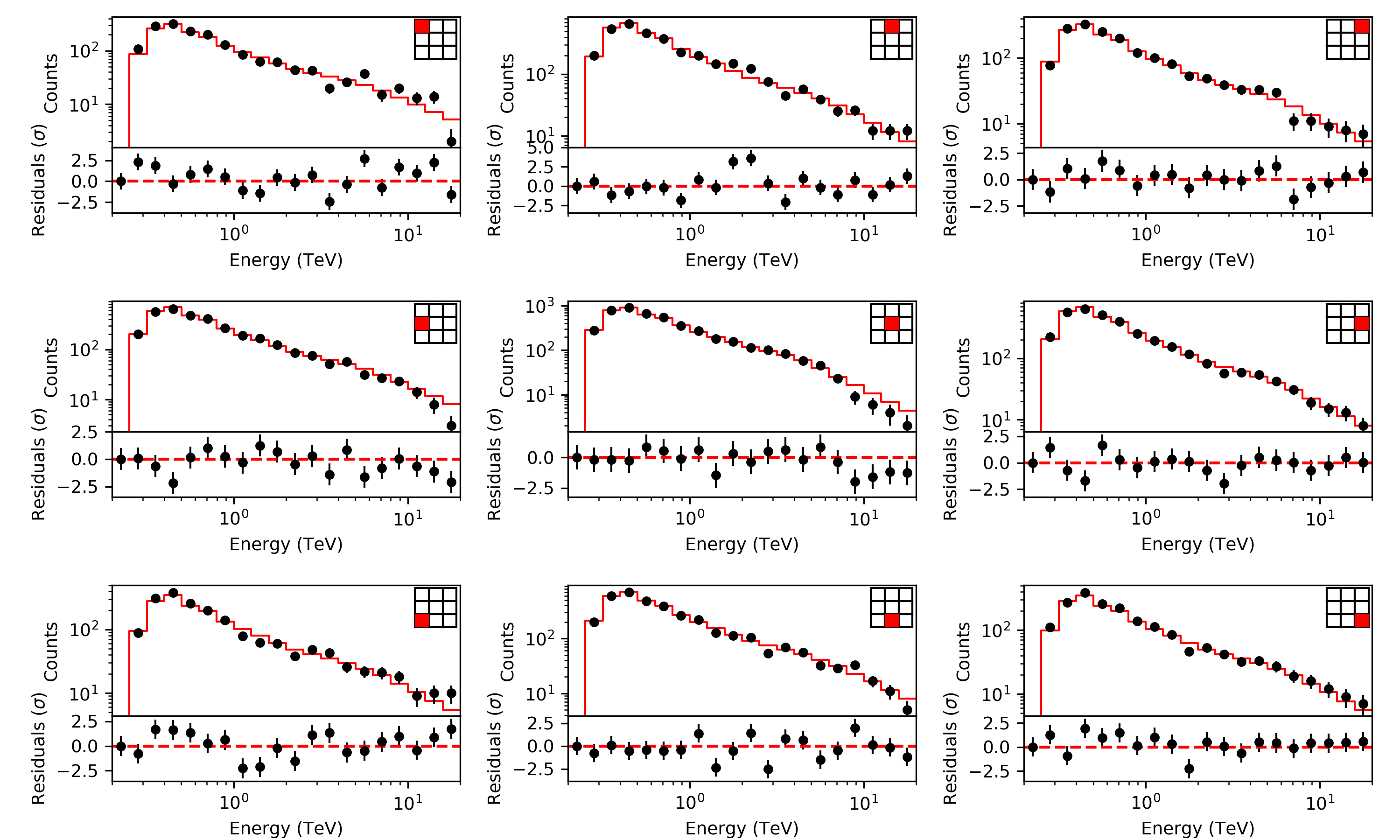
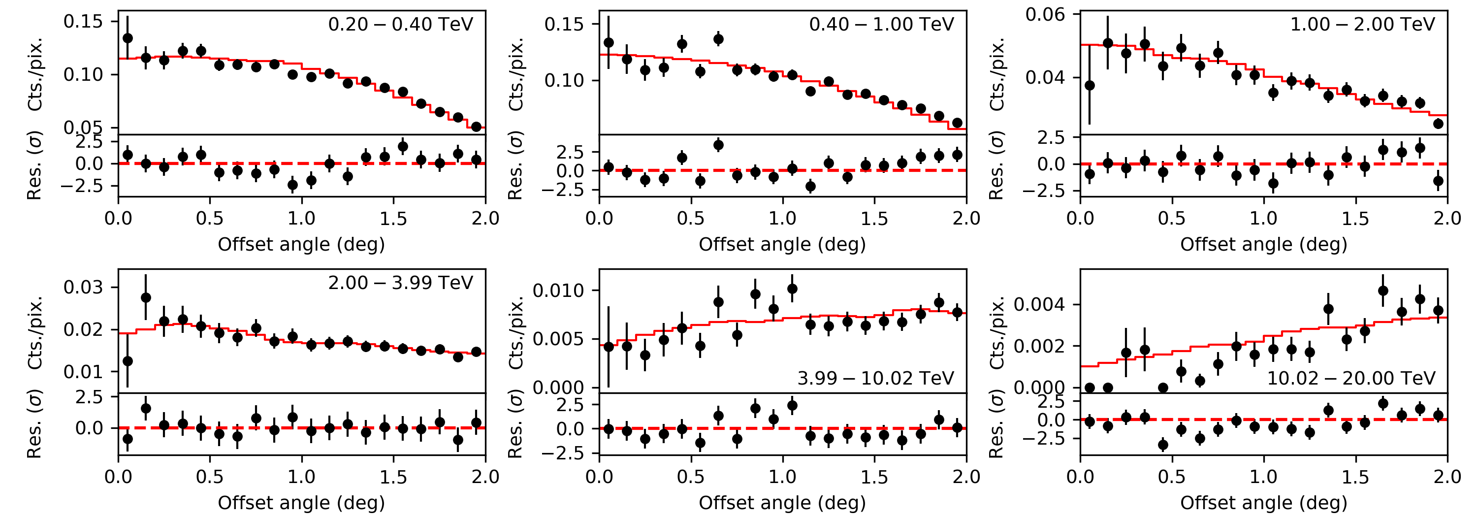
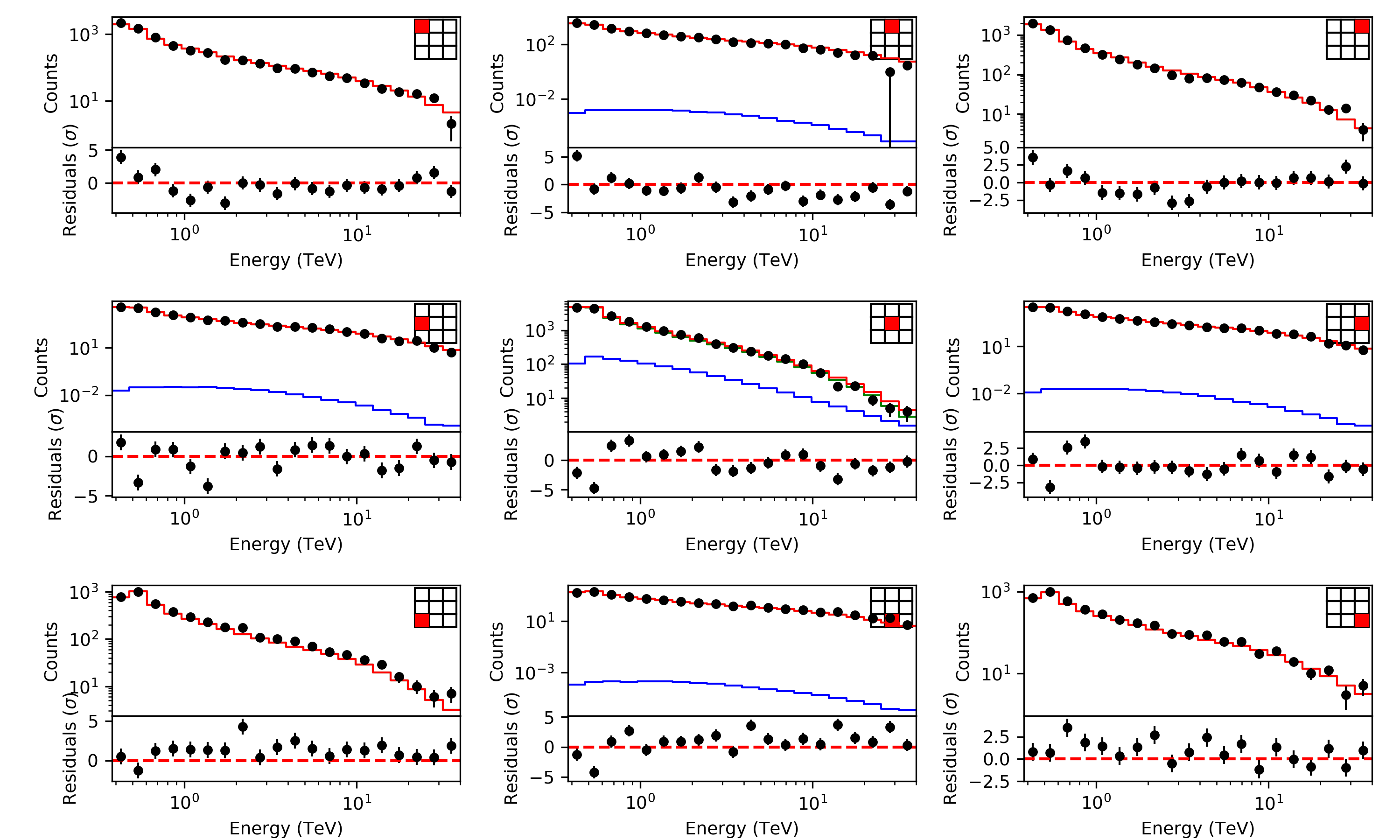
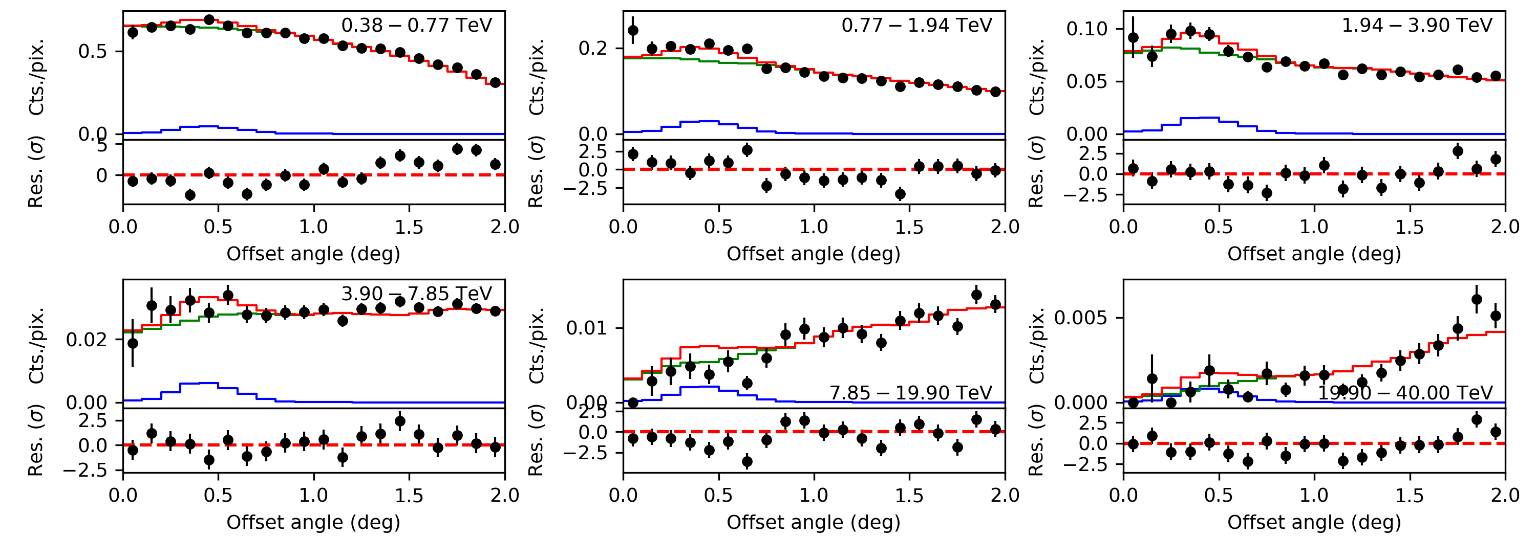
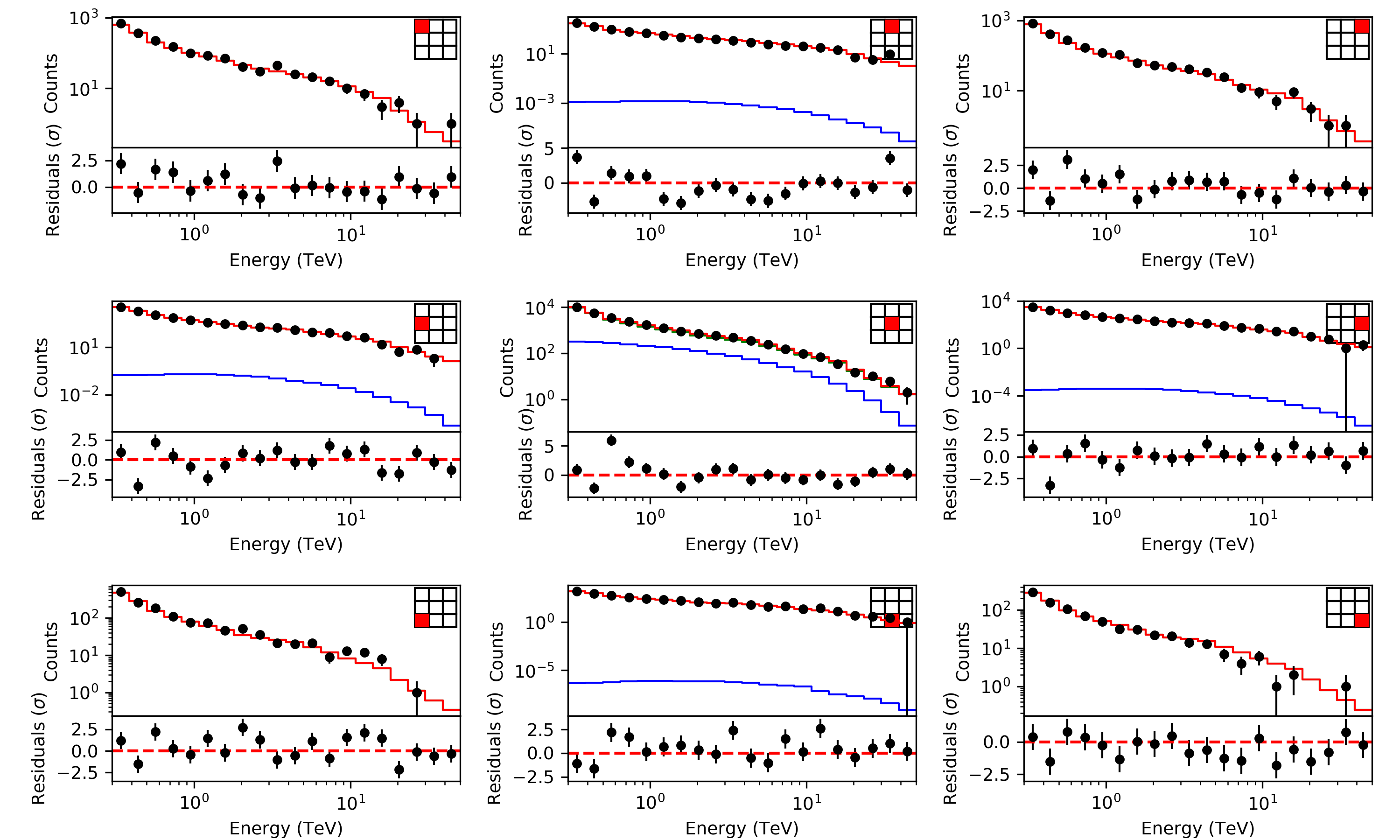
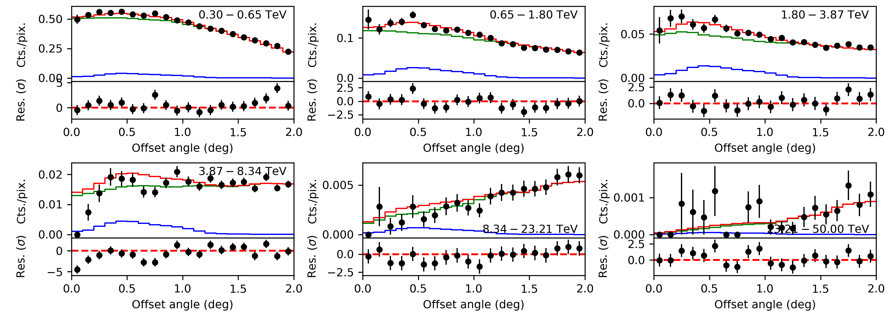
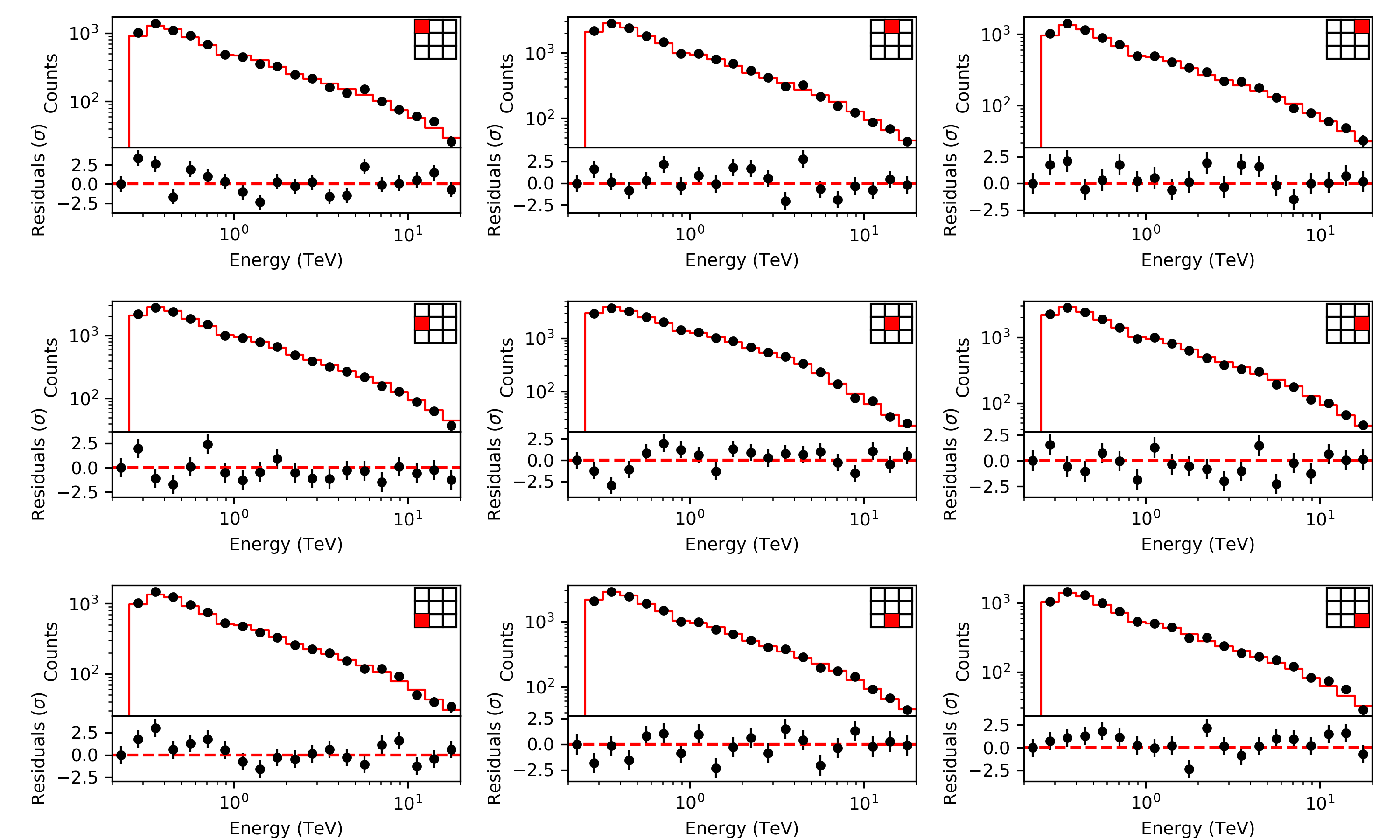
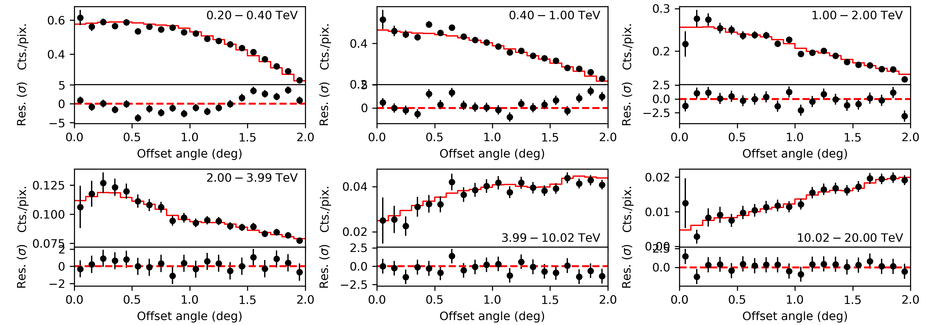
We fitted this background model to each empty-field observation using the unbinned maximum likelihood algorithm implemented in ctlike (see Appendix B for a description of the algorithm). After fitting we performed a visual inspection of the fit residuals for each observation, as well as for all 45 empty-field observations stacked together in the field-of-view coordinate system. Figure 3 shows the spectral residuals, integrated over the field of view, and the spatial residuals, integrated over energy, for the stacked observations. Figure 4 shows the spectral residuals of the stacked observations for the field of view divided into a grid of $3\times 3$ sub-regions of equal size to verify that there are no significant spatial variations in the residuals over the field of view. Figure 5 shows the radial counts profiles and residuals as a function of offset angle $\theta$ for six energy bands. Overall the residuals look reasonably flat, and, although sometimes the scatter is larger than expected from purely statistical fluctuations, no strong trends or biases are apparent. As we will show later in the analysis of MSH 15–52 and RX J1713.7–3946, where the background model is most relevant due to the faintness of the gamma-ray source emission, our analysis results will turn out to not be significantly affected by this scatter.

To ensure that the model can be reliably applied to observations different from those used in the lookup table generation, we furthermore checked the residuals for five subsets of ten stacked empty-field observations that were randomly selected. We generated a background model for each of the ten observations using a lookup table that was based on the remaining 35 empty-field observations, and hence the selected empty-field observations are statistically independent of the background lookup table. Figures 23 – 37 in Appendix E show the corresponding residual plots. In all cases, the spectral, spatial, radial and sub-region residuals look acceptably flat, although some deviations beyond the level expected from statistical fluctuations is once more clearly visible.

Therefore, in the rest of the paper we adopted the csbkgmodel background model each time a background model was required. We ran the script on the observation definition file of each source to produce a model definition file that defines an initial model for the distribution of the background events. The script was run with the runwise option so that an independent background model component is generated for each observation. In this initial iteration of the background-model fitting we did not include a model for the gamma-ray source. This yields a reasonable approximation of the background model parameters because the events recorded over the field of view are in general dominated by background. This implies, however, that the initial model overestimates the background if gamma-ray emission is present. In the next sections the background model will be refined for each source by fitting it to the data together with models for the gamma-ray signal. We checked by inspecting the residuals that the final model for source and background provided a good representation of the data.

2.4 Crab nebula observations

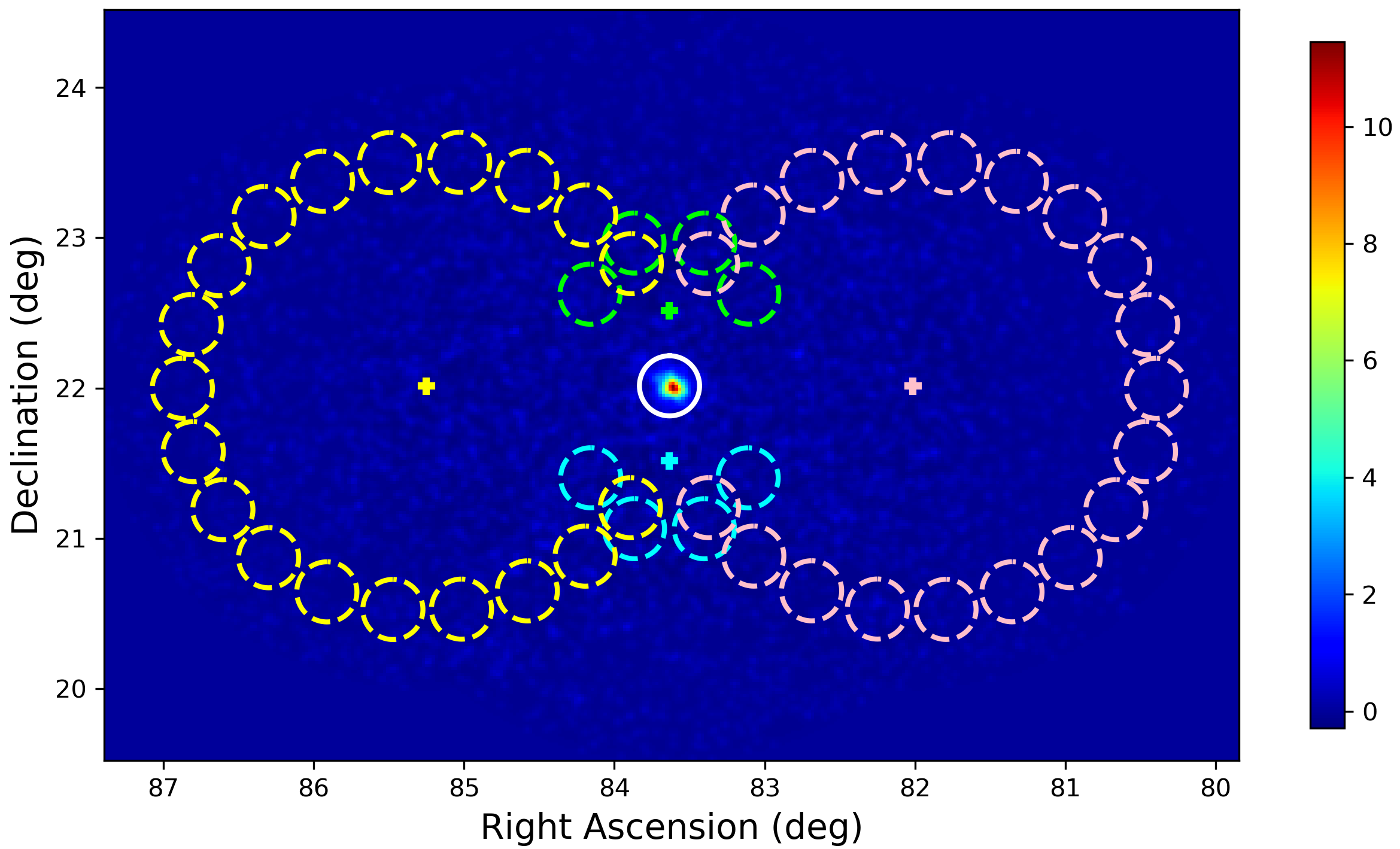
The Crab nebula was the first very-high energy gamma-ray source detected (Weekes et al. 1989) and is one of the brightest objects in the TeV sky. According to previous H.E.S.S. analyses, the source spectrum is well described by an exponentially cut-off power law (Aharonian et al. 2006a) and the source is spatially resolved (Holler et al. 2017). Figure 6 shows a background-subtracted counts map of the Crab nebula observations, using the background model that was fitted to the data in the unbinned maximum likelihood analysis. The On and Off regions used for the classical analysis are also indicated (see below).

We started our analysis by fitting the Crab nebula observations using the unbinned maximum likelihood algorithm implemented in ctlike. Event energies between 670 GeV and 30 TeV were considered. Energy dispersion, which is the probability density of measuring an event energy of $E^{\prime}$ if the true energy is $E$, was accounted for, which was done for all analyses presented in this paper. We used a point-source spatial model for the Crab nebula to allow for comparison of our results with literature values. The position parameters were left free in the model fit, and we tested several spectral models, including a power law (PL) $I(E)=k_{0}(E/E_{0})^{-\Gamma}$, a power law with exponential cut-off (EPL) $I(E)=k_{0}(E/E_{0})^{-\Gamma}\exp(-E/E_{c})$, and a curved power-law model (CPL) $I(E)=k_{0}(E/E_{0})^{-\Gamma+\beta\ln(E/E_{0})}$, also known as log-parabola model. The reference energy $E_{0}$ for all models was set to 1 TeV.

Figure 6: Background-subtracted counts map of the Crab nebula observations for the energy band 670 GeV – 30 TeV. The map was computed for a $0.02^{\circ}\times 0.02^{\circ}$ binning and was smoothed with a Gaussian kernel of $\sigma=0.02^{\circ}$ to reduce statistical noise. The colour bar represents the number of excess counts per bin. The white circle indicates the On region selected for On-Off analysis, coloured dashed circles are the corresponding Off regions and plus symbols the pointing directions, where each colour corresponds to one of the four observations. Coordinates are for the epoch J2000.

The fit results are summarised in Table 2. We measured the detection significance of the source model using the so-called Test Statistic (TS) which is defined as

$$\mathrm{TS}=2\ln L(M_{s}+M_{b})-2\ln L(M_{b})$$ (5)

(Mattox et al. 1996), where $\ln L(M_{s}+M_{b})$ is the log-likelihood value obtained when fitting the source and the background models together to the data, and $\ln L(M_{b})$ is the log-likelihood value obtained when fitting only the background model to the data. Under the hypothesis that the background model $M_{b}$ provides a satisfactory fit of the data, TS follows a $\chi^{2}_{n}$ distribution with $n$ degrees of freedom, where $n$ is the number of free parameters in the source model component. Therefore,

$$p=\int_{\mathrm{TS}}^{+\infty}\chi^{2}_{n}(x)\>\>\mathrm{d}x$$ (6)

gives the chance probability (p-value) that the log-likelihood improves by TS/2 when adding the source model $M_{s}$ due to statistical fluctuations only (Cash 1979).

Table 2: Fit results from the unbinned analysis for the Crab nebula observations for different spectral models assuming a point-source spatial model.

Model	TS	$N_{\rm src}$	$k_{0}$	$\Gamma$	$E_{c}$ or $\beta$
PL	$2021.3$	$684$	$4.5\pm 0.2$	$2.64\pm 0.07$	-
EPL	$2030.6$	$686$	$5.0\pm 0.4$	$2.22\pm 0.18$	$7.4\pm 3.2$
CPL	$2029.9$	$686$	$4.5\pm 0.2$	$2.24\pm 0.16$	$-0.23\pm 0.09$
EPL	n.c.	$4283$	$3.84\pm 0.09$	$2.41\pm 0.04$	$15.1\pm 2.8$
CPL	n.c.	n.c.	$4.47\pm 0.29$	$2.23\pm 0.18$	$-0.16\pm 0.10$

The largest TS value is obtained for the exponentially cut-off power law, and the TS difference of $9.3$ compared to the power-law model corresponds to a significance level of $3.1\sigma$ for the detection of the cut off. The curved power law gives a similar improvement, and statistically the model can not be distinguished from the exponentially cut-off power law. We can compare these results to the values published by Aharonian et al. (2006a) for their dataset III, which covers the period during which the observations of the H.E.S.S. public data release were taken, but which span a much longer live time of 10.6 hours compared to the 1.75 hours analysed in this paper. For dataset III, Aharonian et al. (2006a) quote $4283$ excess counts from the Crab nebula for standard selection cuts, which corresponds to $404$ counts per hour live time, giving an expected number of $707$ excess counts for our dataset. This estimate is in excellent agreement with our $N_{\rm src}$ values in Table 2.

For dataset III, Aharonian et al. (2006a) obtain $k_{0}=(3.84\pm 0.09)\times 10^{-11}$ ph cm^-2 s^-1 TeV^-1, $\Gamma=2.41\pm 0.04$ and $E_{c}=15.1\pm 2.8$ TeV for a power law with exponential cut-off. Fitting the data with a source model where we fixed the spectral parameters to the values of Aharonian et al. (2006a) resulted in a TS value of $2007.2$ that is lower by $23.4$ with respect to our best fitting exponentially cut-off power law. This TS difference corresponds to a significance level of $4.4\sigma$, suggesting that our result differs significantly from the one found by Aharonian et al. (2006a). However, Nigro et al. (2019) analysed the same dataset that we did using conventional IACT analysis techniques, and for a curved power-law model they obtain $k_{0}=(4.47\pm 0.29)\times 10^{-11}$ ph cm^-2 s^-1 TeV^-1, $\Gamma=2.39\pm 0.18$ and $\beta=-0.16\pm 0.10$, which is compatible within statistical errors with our results. Fitting a curved power-law model using their spectral parameters resulted in a TS value of $2028.7$ that is smaller by only $1.2$ with respect to our best-fitting value, corresponding to a significance level of $1.1\sigma$, which confirms that our analysis is consistent with theirs. This suggests that the difference with respect to Aharonian et al. (2006a) should be attributed to differences between their dataset III and the dataset included in the H.E.S.S. public data release. Firstly, the live time of their dataset is six times longer than the live time of the data analysed in this work; hence their sample is statistically different from ours. Secondly, the event reconstruction and background reduction software that was used to prepare the data differs, implying that we do not really analyse the same events. And thirdly, the instrument response functions that were used to recover the physical source parameters are different, which may also explain differences in the fitted spectral parameters. This illustrates the limitations of the comparison of the ctools results with published literature values, and emphasises the need for reference results for the H.E.S.S. public data release.

Figure 7: Crab nebula SED derived using csspec. Red data represent the unbinned csspec analysis, the red curve is the curved power-law model fitted by ctlike, and the light red band is the 68% confidence level uncertainty band of the model fit that was determined using ctbutterfly. The blue curve is the power law with exponential cut-off obtained by Aharonian et al. (2006a) for dataset III, and the green curve is the curved power-law obtained by Nigro et al. (2019).

Table 3: Fit results for the Crab nebula observations under variations of the analysis method assuming a point source with an exponentially cut-off power-law spectrum.

Analysis method	TS	$N_{\rm src}$	$k_{0}$	$\Gamma$	$E_{c}$
H.E.S.S. published	n.c.	$4283$	$3.84\pm 0.09$	$2.41\pm 0.04$	$15.1\pm 2.8$
Unbinned	$2030.6$	$686$	$5.0\pm 0.4$	$2.2\pm 0.2$	$7.4\pm 3.2$
Joint binned	$1967.5$	$664$	$5.0\pm 0.4$	$2.2\pm 0.2$	$6.9\pm 2.9$
Stacked binned	$1918.1$	$651$	$4.8\pm 0.4$	$2.1\pm 0.2$	$6.2\pm 2.5$
Joint On-Off (wstat)	$1134.3$	$562$	$5.0\pm 0.4$	$2.2\pm 0.2$	$6.8\pm 3.4$
Joint On-Off (cstat)	$996.1$	$549$	$4.8\pm 0.4$	$2.2\pm 0.2$	$8.0\pm 4.6$
Stacked On-Off (wstat)	$1359.5$	$575$	$5.0\pm 0.4$	$2.2\pm 0.2$	$7.4\pm 3.6$
Stacked On-Off (cstat)	$1102.7$	$553$	$4.8\pm 0.4$	$2.2\pm 0.2$	$7.2\pm 3.5$

We then used csspec in unbinned analysis mode to derive the spectral energy distribution (SED) of the Crab nebula. csspec performs maximum likelihood model fits for a predefined set of energy bins, where model parameters are independently fit for each energy bin. Since most of the energy nodes of the spectral background model component would actually lie outside a given energy bin, we replaced the energy nodes $B_{i}$ by a simple power law for the csspec analysis, where the power law index was determined by fitting the power law over the full energy range. The spatial parameters $G_{\mathrm{x}}$ and $G_{\mathrm{y}}$ and the spectral power-law prefactor were then fitted independently for each energy bin. Comparing the SED to the fitted model curve then allows an assessment of the impact on the analysis results of the choice of the functional form for $B_{\mathrm{spectral}}(E^{\prime})$ and the assumed energy independence of the spatial gradient.

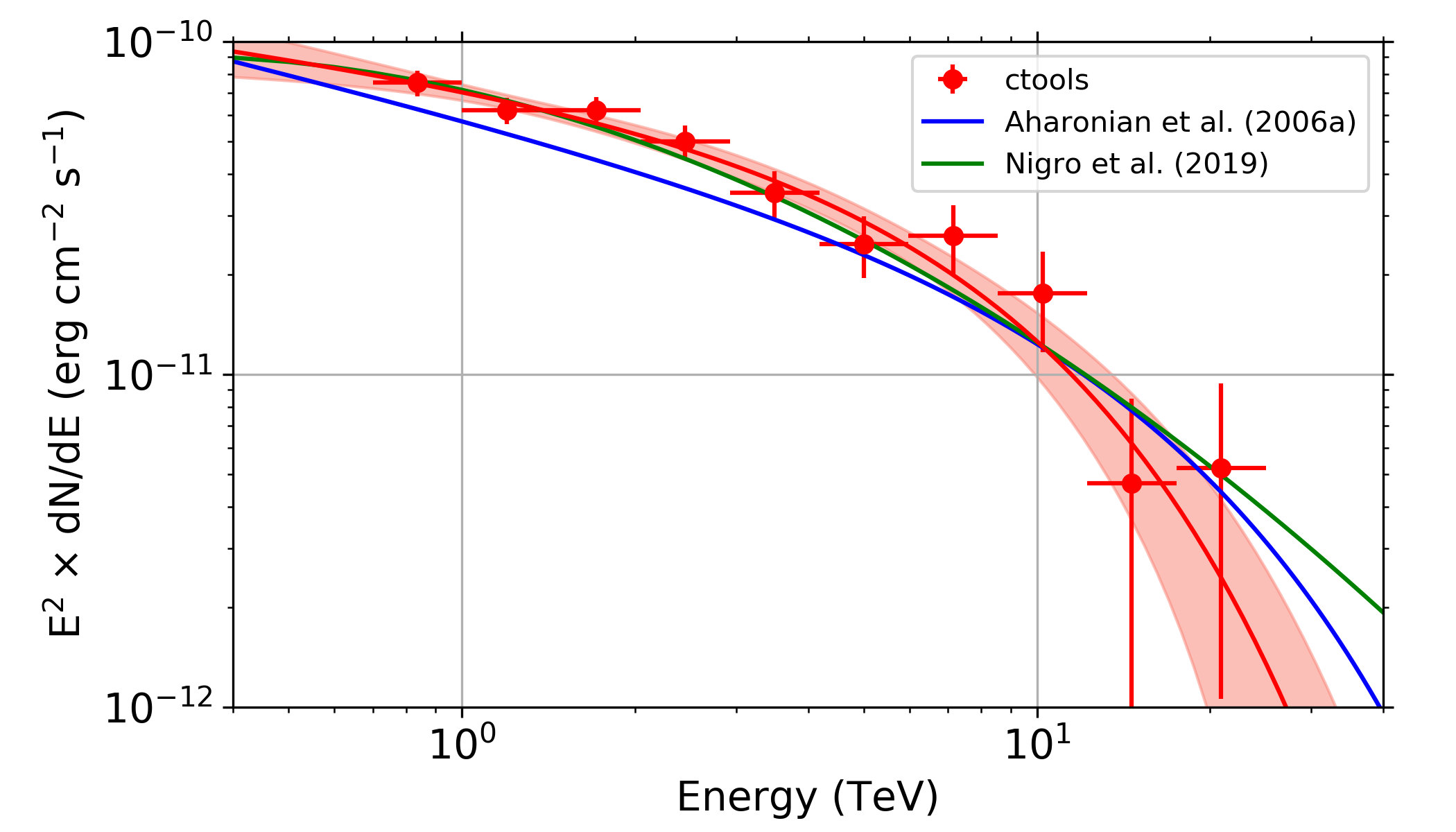
The SED derived using csspec for the Crab nebula observations is shown in Fig. 7. The figure also shows a butterfly diagram of the curved power-law that we generated using ctbutterfly in unbinned analysis mode. The SED nicely follows the curved power-law spectrum, demonstrating that the spectral results are robust with respect to the specific parametrisation of the background model. For comparison, we also show the power law with exponential cut-off obtained by Aharonian et al. (2006a) for dataset III, and the curved power-law obtained by Nigro et al. (2019). The published H.E.S.S. result differs significantly from our best-fitting spectrum, but as explained above, several reasons could explain this discrepancy. Our spectrum is however in excellent agreement with the spectrum of Nigro et al. (2019) that was based on the same data, confirming the good agreement between the analysis results.

The results we have presented to this point were obtained using an unbinned maximum likelihood fitting method. The ctools offer alternative analysis methods, including a joint binned analysis, where the events for each observation are filled into a 3D counts cube spanned by Right Ascension, Declination, and the logarithm of the reconstructed energy, and a stacked binned analysis, where the events of all observations are combined into a single 3D counts cube and the effective response for the stacked cube is computed and used. Collectively we call these methods 3D analyses.

Figure 8: Gamma-ray extension, given as the $1\sigma$ radius of a 2D Gaussian fit, of the Crab nebula as derived from Holler et al. (2017) (blue) and using ctools (red) superimposed on a Chandra 0.3–10 keV X-ray image of the Crab nebula (credit: NASA/CXC/SAO). The crosses indicate the statistical uncertainty in the centroid position as quoted by Holler et al. (2017) (blue) and as derived from the Gaussian model fitting using ctlike (red). The systematic positioning accuracy of H.E.S.S. of $20^{\prime\prime}$ (Holler et al. 2017) is indicated as a white circle. Coordinates are for the epoch J2000.

Figure 9: Residuals after fitting the Crab observations using a 2D Gaussian spatial model with an exponentially cut-off power-law spectrum using an unbinned maximum likelihood fit. The leftmost panel shows the counts and model spectra and the residuals after subtraction of the source and background models for the On region. The second panel shows the spectra and residuals for the entire field of view. In both panels, red lines represent the total predicted model counts, blue lines the predicted source counts and green lines the predicted background counts. The third panel shows the histogram of significances, determined after summing over the spectral dimension and by sampling the events into bins of $0.2^{\circ}\times 0.2^{\circ}$. A Gaussian was fitted to the significance histogram, and the best fitting mean and width of the Gaussian are given together with the statistical fit errors in the plots. Perfect residuals would lead to a mean of zero and a width of unity. The rightmost panel shows a residual significance map summed over all energies for a correlation radius of $0.2^{\circ}$. The map is in significance units expressed in Gaussian $\sigma$.

In addition On-Off analyses are also supported, where only the data from an On region are analysed and the background is estimated from one or several Off regions. The On-Off analysis, which corresponds to the classical technique for analysing data from IACTs, exists in several variants. Firstly, observations can either be analysed jointly or stacked. For a joint analysis, On-Off spectra from individual observations are kept separately and a joint maximum likelihood fitting is performed using the effective instrument response for the On region of each observation. For a stacked analysis, all events from individual observations are combined into a single On and a single Off spectrum, and the resulting effective instrument response for the combined observations is used in the maximum likelihood fitting.

Secondly, maximum likelihood fitting can be either performed using the wstat or the cstat statistic (see Appendix C.2). For wstat, it is assumed that the background rate per solid angle is identical in the On and Off regions, and hence no explicit background model is needed for the analysis. Such a situation may occur if the On and Off regions are symmetrically located around the pointing direction, provided that background gradients over the field of view are negligible. Conversely, for cstat, a background model is used to describe the background rate differences between On and Off regions that may occur if the regions are not symmetrically located around the pointing direction, or in the presence of significant background gradients. For this paper, we used the background model produced by csbkgmodel for the cstat analysis, with individual components for each observation for the joint case, and a single component for the stacked case. The On-Off analysis methods are described in more detail in Appendix C. We note that for each observation, the cstat analysis has the eight background rates $B_{i}$ as free parameters, while the wstat analysis implicitly has one background rate per energy bin as nuisance parameters.

Table 3 summarises the Crab nebula spectral fitting results for a point source with an exponentially cut-off power-law spectrum. All spatial and spectral source parameters, as well as the parameters of the background model, were free parameters in the model fits, except for the On-Off analyses, which do not consider the spatial source and background components and consequently do not allow for an adjustment of the corresponding parameters. Spatial bins of $0.02^{\circ}\times 0.02^{\circ}$ and 40 logarithmically spaced energy bins were used for the binned analysis, with $200\times 200$ bins around the pointing direction of each observation for the joint analysis, and $350\times 250$ bins around the Crab nebula position (Right Ascension $83.63^{\circ}$ and Declination $22.01^{\circ}$) for the stacked analysis. The same number of energy bins was also used for the On-Off analysis, and the On region was defined as a circle of $0.2^{\circ}$ in radius centred on the Crab nebula position. The reflected regions method was used to define the Off regions (Berge et al. 2007). The On region and reflected Off regions are shown for illustration in Fig. 6.

As can be seen from Table 3, all analysis methods give compatible results. The results for the joint binned analysis are very close to those for the unbinned analysis, validating the consistent implementation of both analysis methods in the ctools package. Also the stacked binned analysis gives comparable results, although the background model for this analysis was generated by stacking the initial background models obtained for each observation which ignore any source contributions, and thus formally overestimate the background in case that some source emission is present. The nevertheless good agreement with the other analyses can be explained by the fact that, even for observations of a strong source like the Crab nebula, the field-of-view integrated counts are largely dominated by background (cf. Fig. 9). In addition, the stacked background model is renormalised during the source fitting, compensating to a large extent the initial overestimation of the background model.

The On-Off analysis results are close to those obtained with the 3D analyses, providing an important cross-check between our novel analysis approach with the classical IACT analysis methods. The number of source events for the On-Off analyses are about $20\%$ smaller compared to the 3D analyses, which is in agreement with the fraction of events that are found in the tail of the point-spread function beyond the On region cut of $0.2^{\circ}$. We also note that results obtained using wstat are compatible with those obtained using cstat, suggesting that details of the background model affect only marginally the Crab analysis, which is understandable since the events in the On region are largely dominated by the source (cf. Fig. 9). Finally, the stacked On-Off analyses provide results that are compatible with the joint On-Off analyses, demonstrating once again that the loss of information due to the stacking of individual observations does not substantially degrade the analysis results.

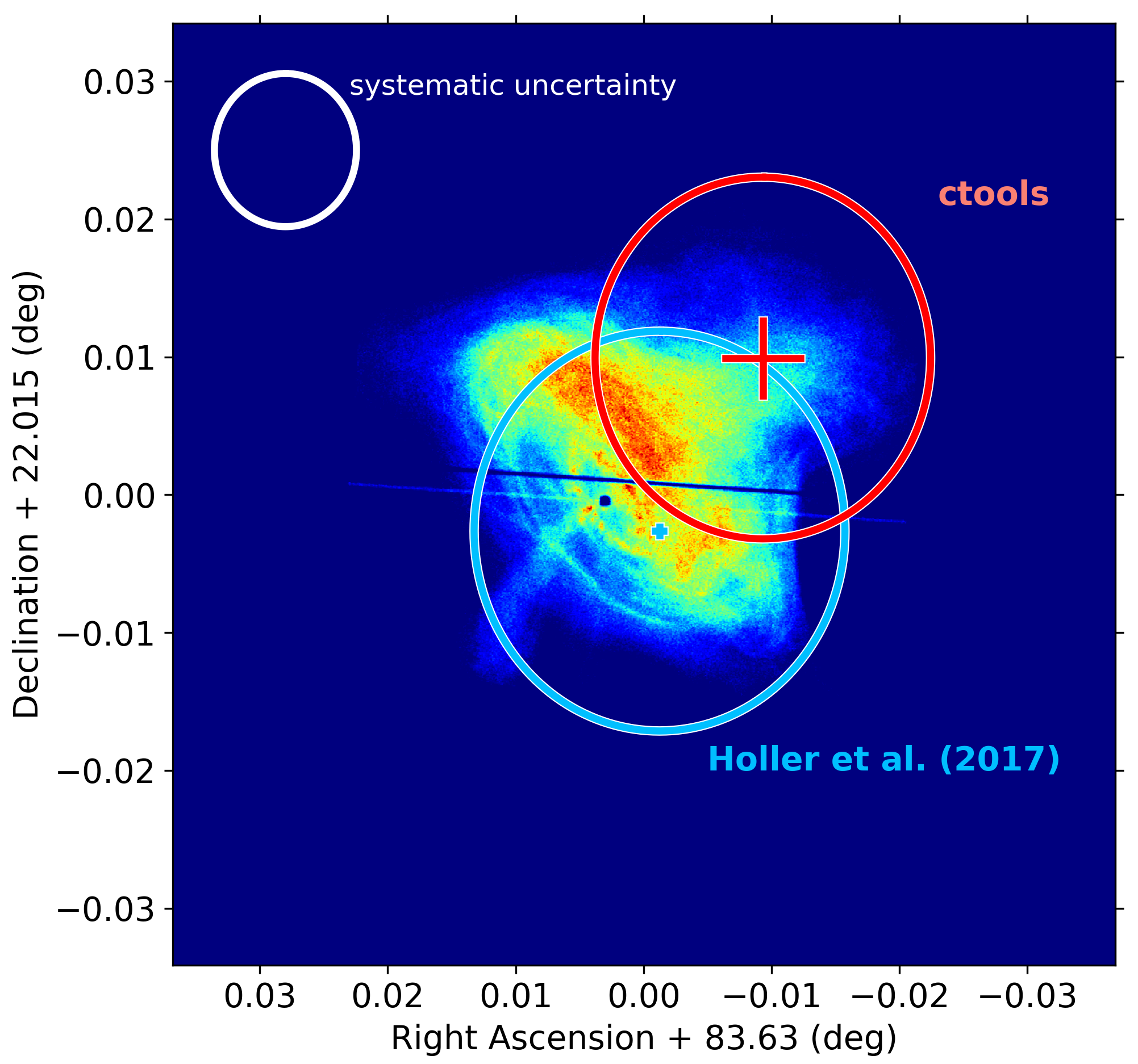
As next step we investigated the morphology of the Crab nebula. Using a dedicated analysis, Holler et al. (2017) reported recently the measurement of the extension of the Crab nebula, and although the Instrument Response Functions (IRFs) in the H.E.S.S. data release have a lower precision compared to those used by Holler et al. (2017), we wanted to check whether we were able to reproduce this result with ctools. We therefore replaced the point-source model by a 2D Gaussian model, similar to the model used by Holler et al. (2017), and fitted the observations using ctlike in unbinned mode. We obtained a 2D Gaussian extent of $\sigma=47^{\prime\prime}\pm 18^{\prime\prime}$ using a power law with exponential cut-off for the spectral component, which is compatible with the value of $\sigma=52^{\prime\prime}\pm 3^{\prime\prime}$ derived by Holler et al. (2017). Using a power law or curved power law spectral shape for the source changed the extension value by at most $3^{\prime\prime}$. Figure 8 illustrates our result in comparison to the result of Holler et al. (2017), superimposed on a Chandra X-ray image of the Crab nebula. The best-fitting centroid of the 2D Gaussian, which we determined to $83.621^{\circ}\pm 0.003^{\circ}$ in Right Ascension and $22.025^{\circ}\pm 0.003^{\circ}$ in Declination (J2000), is slightly offset from the Crab nebula centre. We did not find such large offsets between H.E.S.S. results and ctools localisations for other sources (see below); hence it is plausible to attribute this offset to systematic uncertainties in the reconstructed H.E.S.S. data and/or response functions.

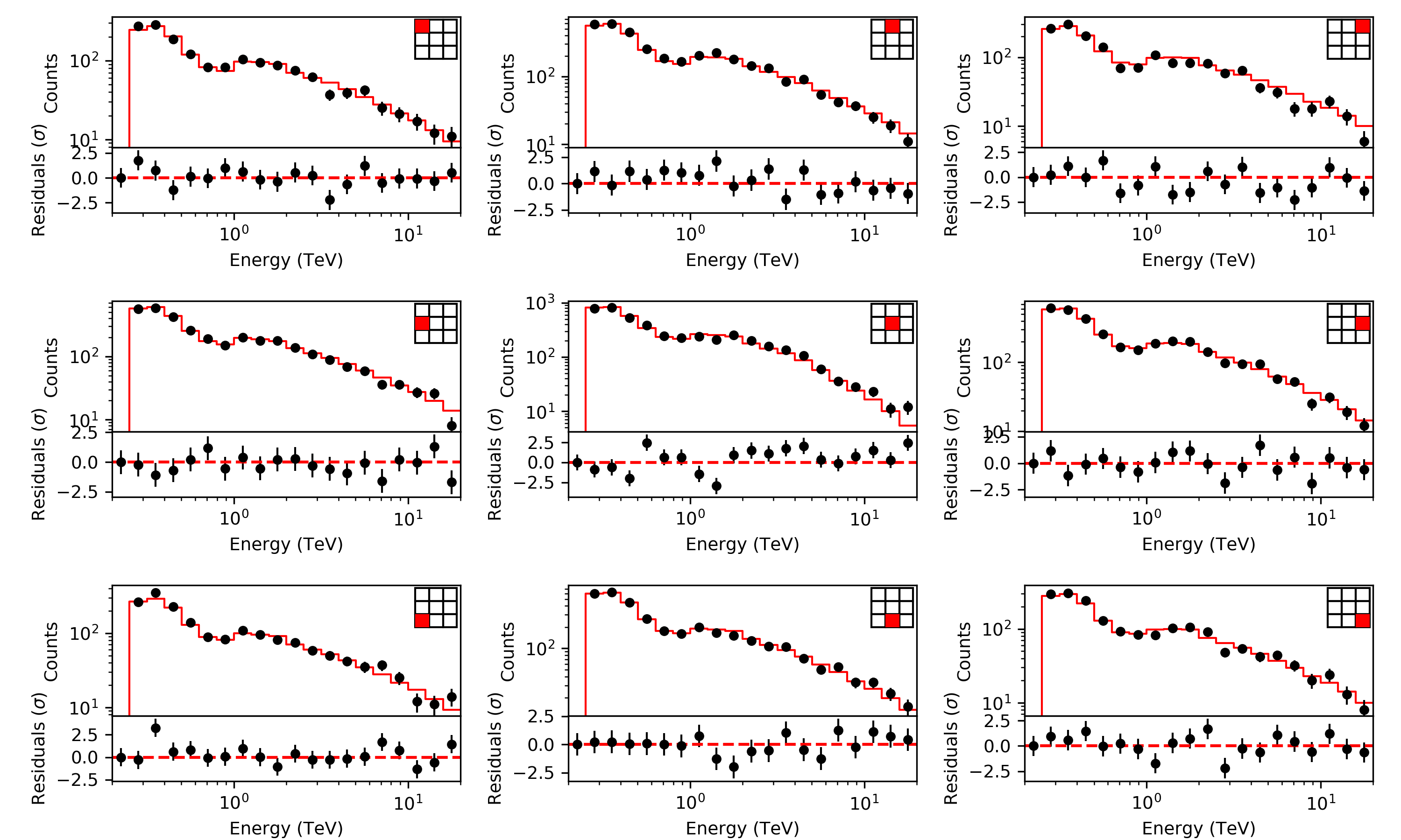
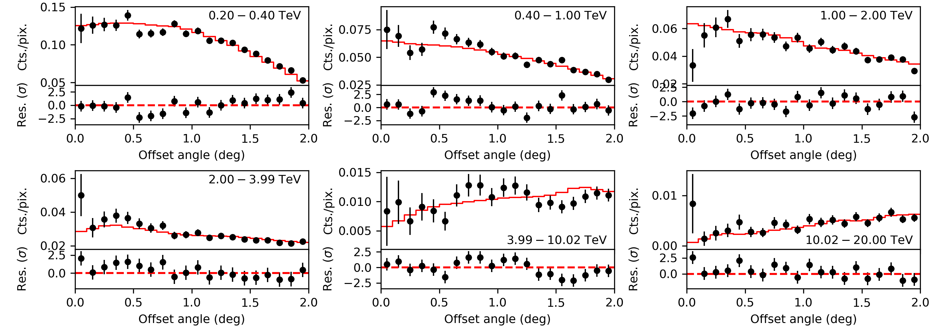
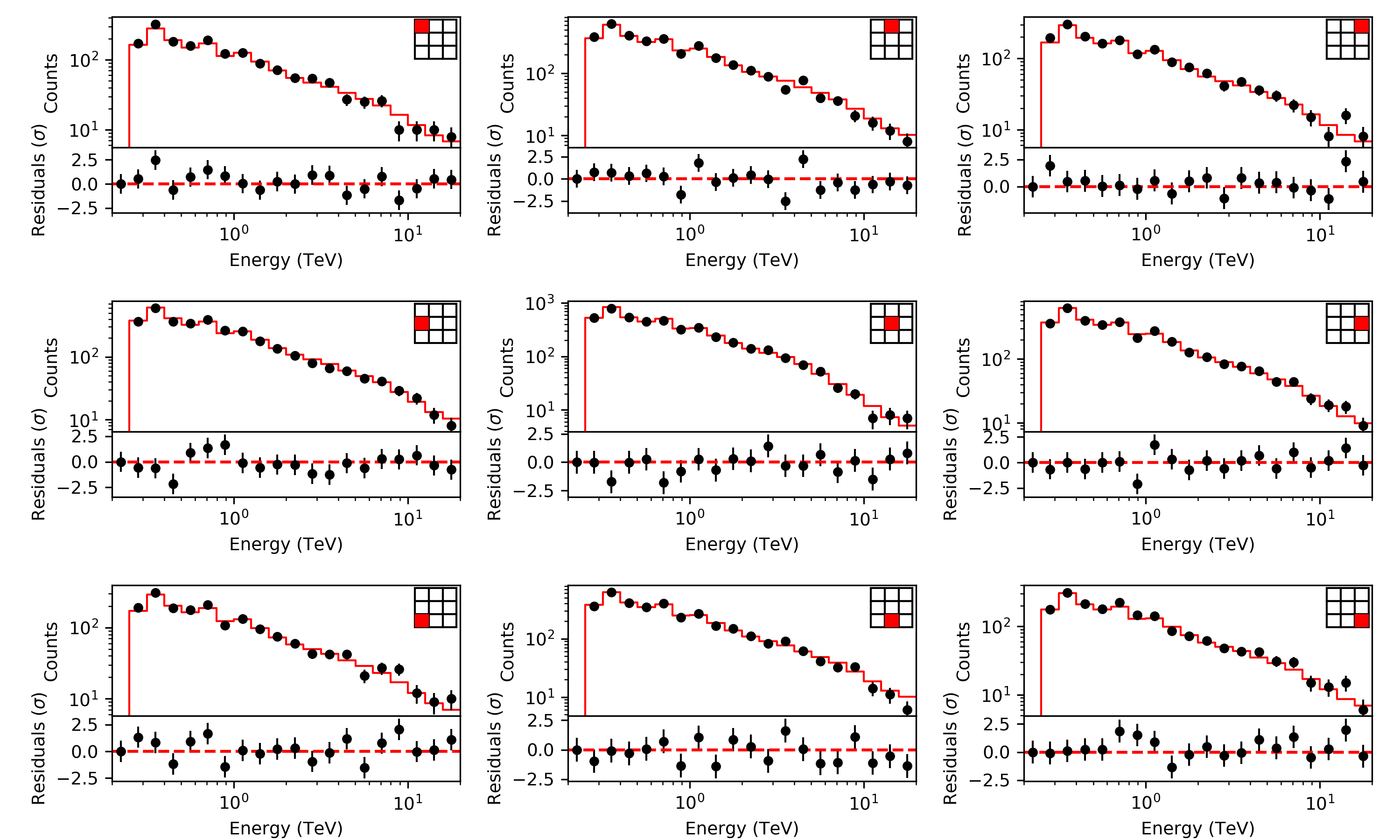
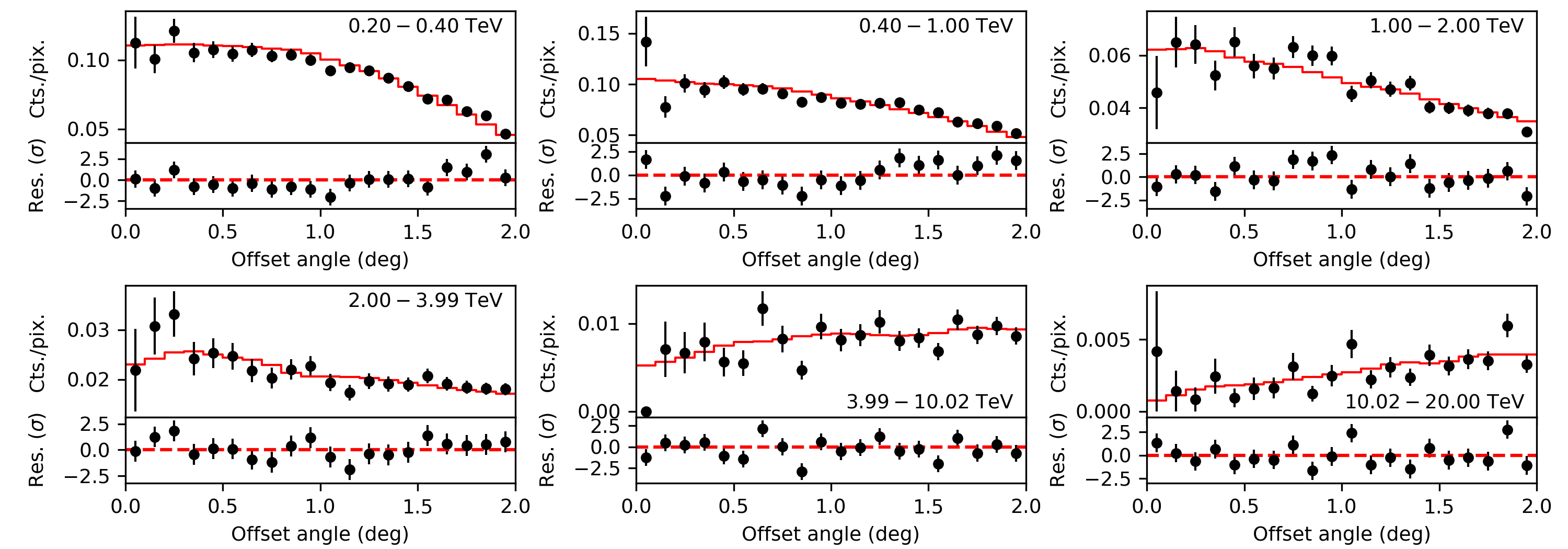
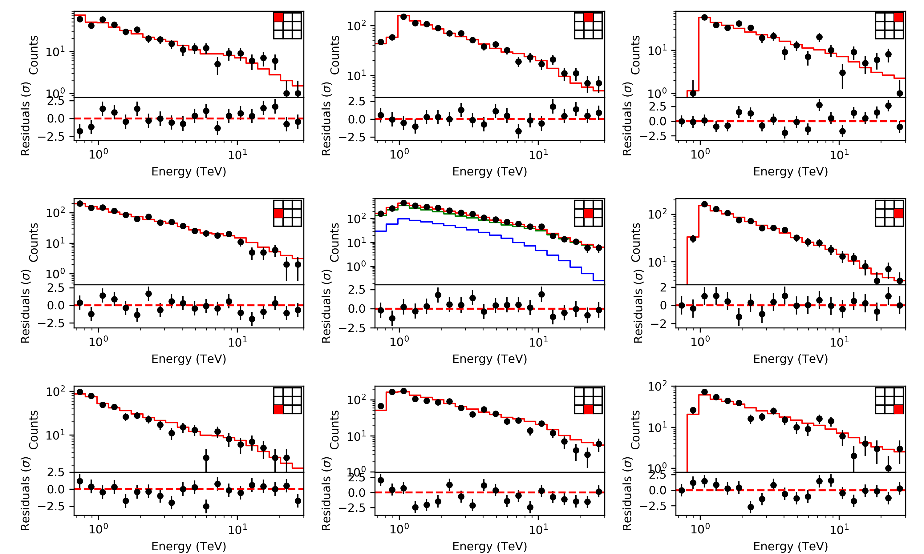
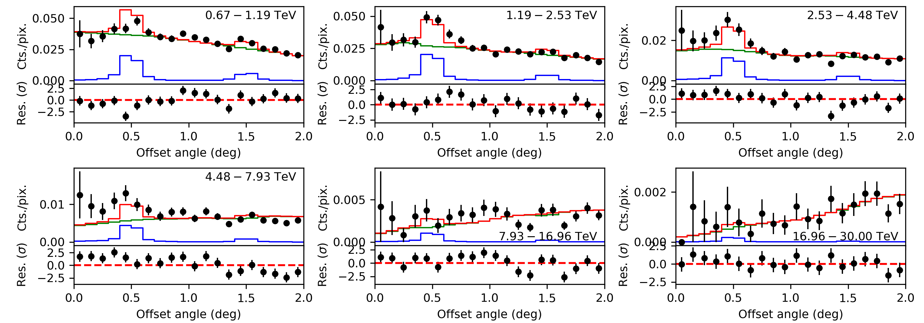
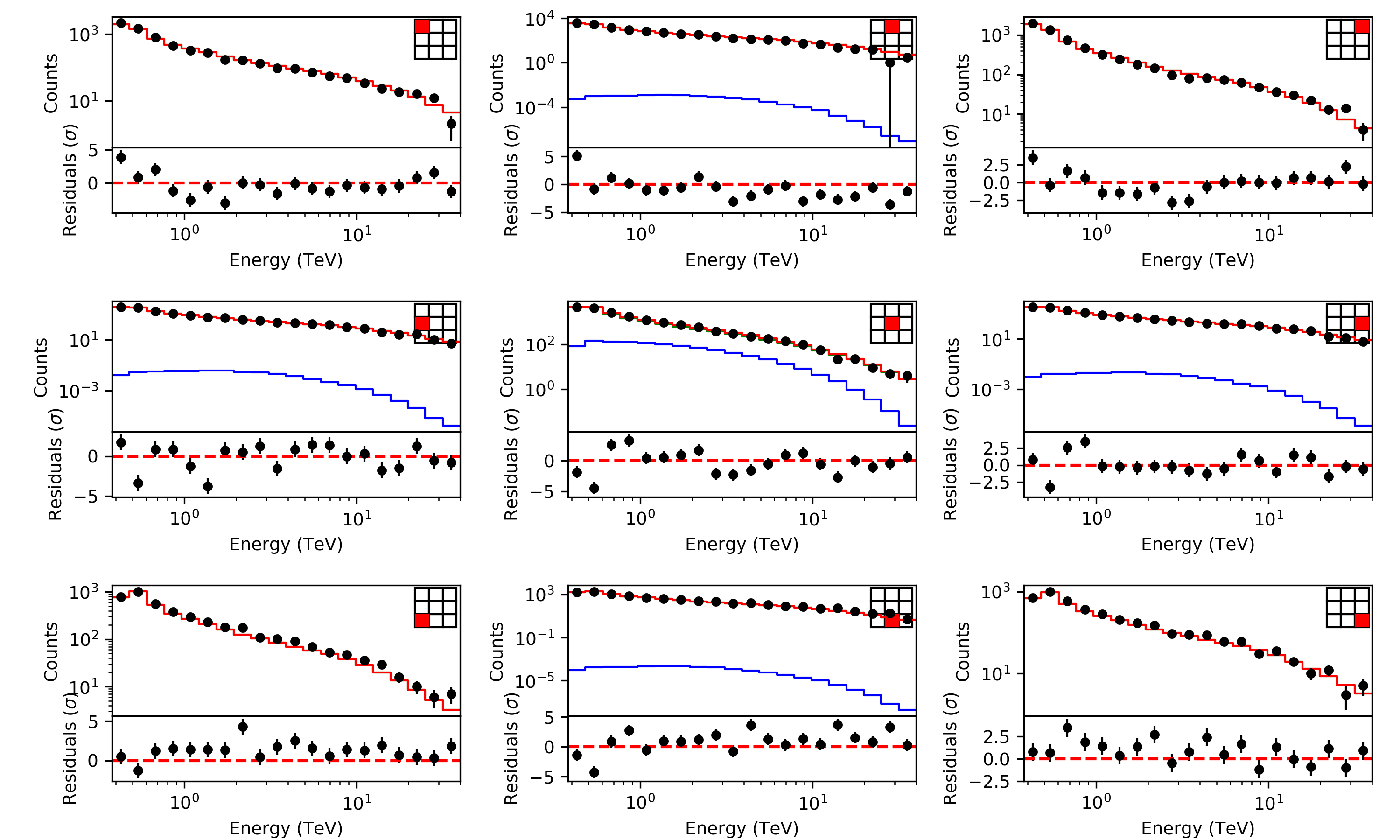
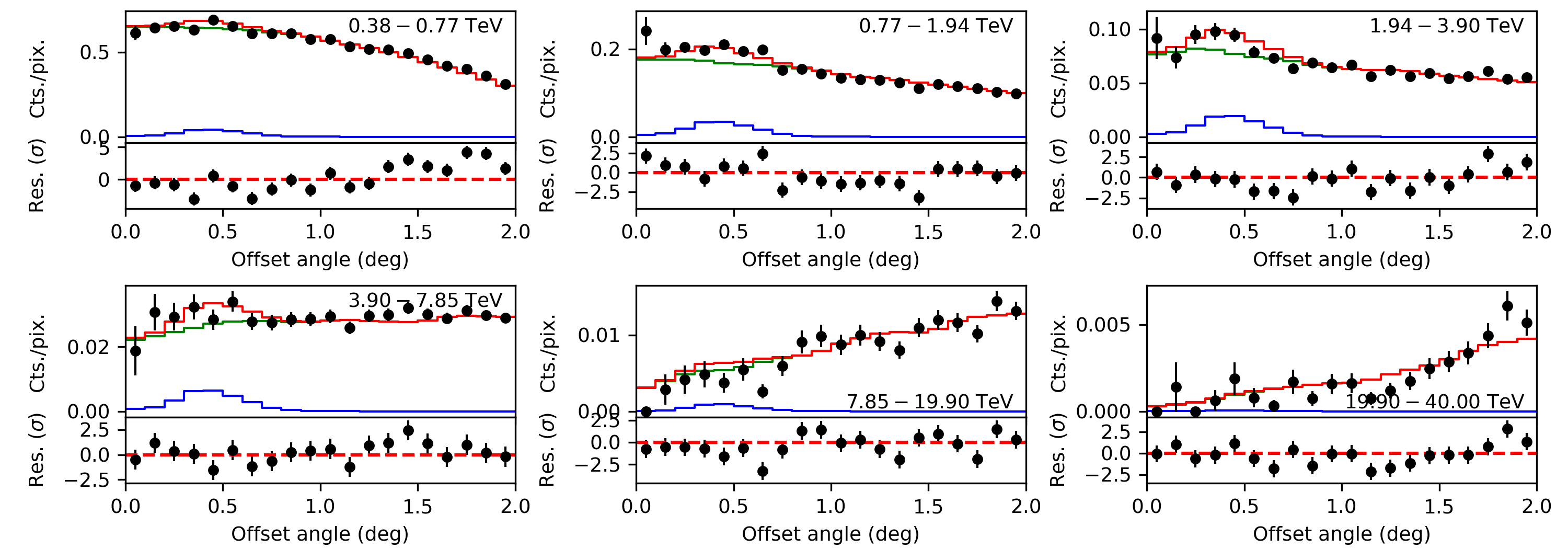
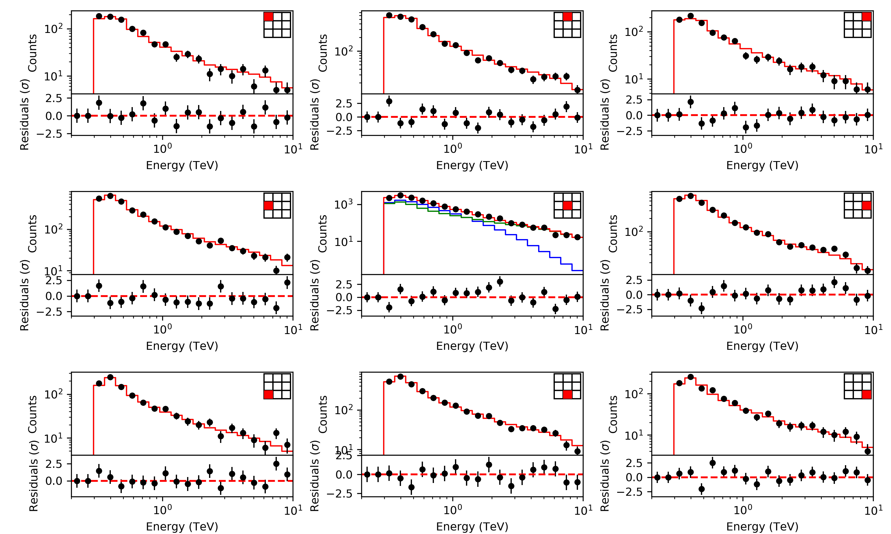
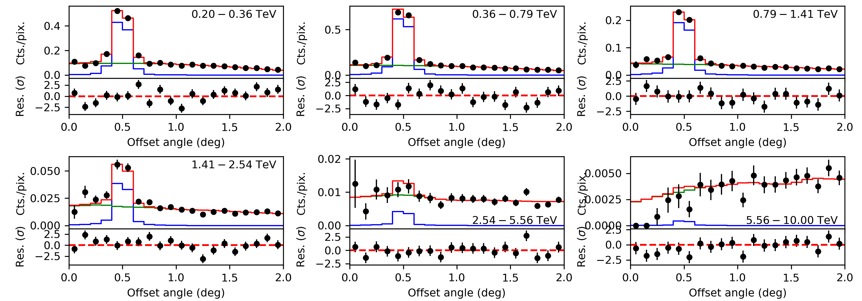
We inspected the spatial and spectral residuals of the fit; corresponding plots are shown in Fig. 9. The spectral residuals are very flat, and also the significance distribution of the residual counts is very close to the expectations. The spatial residuals are also relatively flat and appear to be homogeneously distributed over the field of view. We also examined the spectral residuals for nine spatial sub-regions, and the radial counts profiles and residuals as a function of offset angle $\theta$ for six energy bands. The corresponding plots are shown in Figs. 38 and 39 of Appendix E. The residuals are relatively flat, and in particular, they do not show evidence for any strong biases or trends over the field of view, although fluctuations beyond those expected from pure statistics exist and small trends are discernable.

2.5 MSH 15–52 observations

MSH 15–52 is a radio supernova remnant that houses an X-ray pulsar embedded in a pulsar wind nebula (PWN). The discovery of TeV gamma-ray emission from the MSH 15–52 PWN was reported by Aharonian et al. (2005), which provided the first image of an extended PWN in this energy range. The H.E.S.S. observations revealed a complex emission morphology that was fitted by a two-dimensional Gaussian model with major and minor axes of $6.4^{\prime}\pm 0.7^{\prime}$ and $2.3^{\prime}\pm 0.5^{\prime}$ and a position angle of $139^{\circ}\pm 13^{\circ}$. The H.E.S.S. data were consistent with a power-law spectrum with an index $\Gamma=2.27\pm 0.03$ and a differential flux at 1 TeV of $(5.7\pm 0.2)\times 10^{-12}$ ph cm^-2 s^-1 TeV^-1 (Aharonian et al. 2005).

Table 4: Fit results for the MSH 15–52 observations for different analysis methods.

Analysis method	TS	$N_{\rm src}$	R.A. (deg)	Decl. (deg)	$\sigma_{\rm maj}$	$\sigma_{\rm min}$	PA (deg)	$k_{0}$	$\Gamma$
H.E.S.S. published	n.c.	3481	$228.529\pm 0.006$	$-59.159\pm 0.003$	$6.4^{\prime}\pm 0.7^{\prime}$	$2.3^{\prime}\pm 0.5^{\prime}$	$139\pm 13$	$5.7\pm 0.2$	$2.27\pm 0.03$
Unbinned	$762.1$	$1134$	$228.548\pm 0.012$	$-59.174\pm 0.007$	$6.3^{\prime}\pm 0.5^{\prime}$	$3.7^{\prime}\pm 0.4^{\prime}$	$147\pm 6$	$6.1\pm 0.3$	$2.30\pm 0.06$
Joint binned	$781.1$	$1139$	$228.552\pm 0.012$	$-59.174\pm 0.007$	$6.4^{\prime}\pm 0.5^{\prime}$	$4.0^{\prime}\pm 0.4^{\prime}$	$149\pm 7$	$6.4\pm 0.4$	$2.28\pm 0.06$
Stacked binned	$767.6$	$1124$	$228.548\pm 0.012$	$-59.172\pm 0.007$	$6.6^{\prime}\pm 0.5^{\prime}$	$3.8^{\prime}\pm 0.4^{\prime}$	$148\pm 6$	$6.4\pm 0.4$	$2.26\pm 0.06$
Joint On-Off (wstat)	$440.9$	$870$	$228.548$	$-59.174$	$6.3^{\prime}$	$3.7^{\prime}$	$147$	$6.5\pm 0.4$	$2.35\pm 0.07$
Joint On-Off (cstat)	$527.5$	$877$	$228.548$	$-59.174$	$6.3^{\prime}$	$3.7^{\prime}$	$147$	$6.5\pm 0.4$	$2.30\pm 0.06$
Stacked On-Off (wstat)	$530.1$	$882$	$228.548$	$-59.174$	$6.3^{\prime}$	$3.7^{\prime}$	$147$	$6.5\pm 0.4$	$2.30\pm 0.06$
Stacked On-Off (cstat)	$548.4$	$890$	$228.548$	$-59.174$	$6.3^{\prime}$	$3.7^{\prime}$	$147$	$6.6\pm 0.4$	$2.30\pm 0.06$

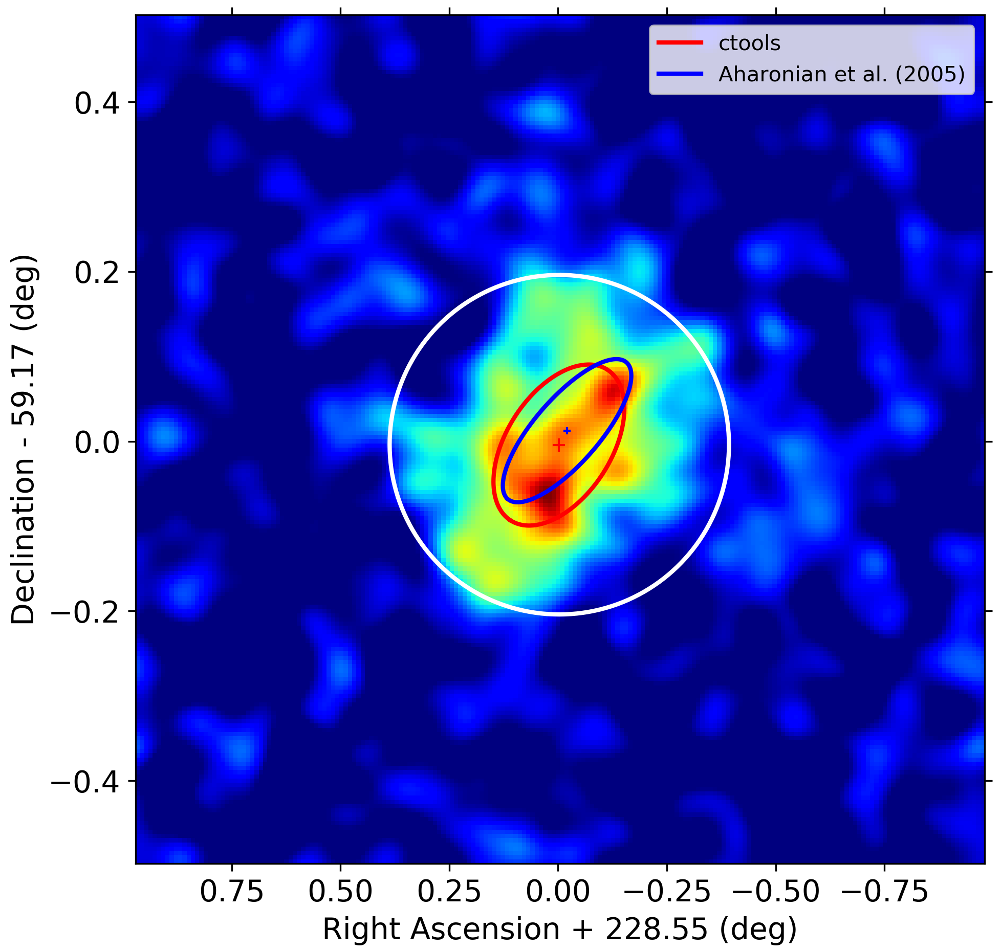
We therefore analysed the MSH 15–52 observations using a source model composed of an elliptical 2D Gaussian for the spatial component and a power law for the spectral component. Events with energies between 381 GeV and 40 TeV were considered. As for the Crab nebula, we performed unbinned and binned 3D maximum likelihood analyses, and the different variants of the On-Off analysis that are available in ctools. The On-Off analyses do not allow the assessment of the spatial source model parameters, hence we fix them for these analyses to the values obtained in the unbinned analysis. For the binned analysis, we used spatial bins of $0.02^{\circ}\times 0.02^{\circ}$, with $200\times 200$ bins around the pointing direction of each observation for the joint analysis, and $200\times 250$ bins around Right Ascension $228.4817^{\circ}$ and Declination $-59.1358^{\circ}$ for the stacked analysis. The energy range was divided into 40 logarithmically spaced energy bins. The same number of energy bins was also used for the On-Off analysis, and an On region of $0.2^{\circ}$ in radius centred on Right Ascension of $228.547^{\circ}$ and Declination of $-59.174^{\circ}$ was used. The Off regions were defined using the reflected regions method. We note that Aharonian et al. (2005) use a larger On region radius of $0.3^{\circ}$ in their work, yet this larger radius does not allow us to define a sufficient number of Off regions for about half of the observations for which the offset angle between MSH 15–52 and the pointing direction amounts to only $0.4^{\circ}$. We therefore decided to use a smaller On region of $0.2^{\circ}$ (see Fig. 10) which probably misses some small fraction of the MSH 15–52 events. Nevertheless, based on the spatial model, csphagen computes the event leakage outside the On region for a given spatial model, and takes it into account when computing the Auxiliary Response File for the analysis (cf. Eq. 18). Consequently, the resulting spectral parameters should reflect the full flux from MSH 15–52 under the assumption that the spatial model adequately describes the gamma-ray emission morphology.

Figure 10: Background-subtracted counts map of the MSH 15–52 observations for the energy band 381 GeV – 40 TeV. The map was computed for a $0.005^{\circ}\times 0.005^{\circ}$ binning and was smoothed with a Gaussian kernel of $\sigma=0.02^{\circ}$ to reduce statistical noise. The $1\sigma$ contour of the elliptical Gaussian fitted using ctools is indicated as a red ellipse. The fit results from Aharonian et al. (2005) are indicated as a blue ellipse. The crosses indicate the statistical uncertainty in the centroid positions. The white circle indicates the On region used in the On-Off analysis. Coordinates are for the epoch J2000.

The results of the ctlike maximum likelihood model fits using different analysis methods are summarised in Table 4. Aharonian et al. (2005) find 3481 excess counts for 22.1 hours of live time within the circular On region of $0.3^{\circ}$ which fully encloses the emission, corresponding to 158 excess counts per hour live time. This rate leads to an estimate of 1307 excess counts for the 8.3 hours of live time included in the H.E.S.S. public data release, which is of the same order as the $N_{\rm src}$ values obtained for the 3D analyses. Our estimates for the On-Off analyses are lower, typically around $\sim 110$ excess counts per hour live time, suggesting that $\sim 30\%$ of the excess counts are lost due to the choice of a smaller On region in our analysis with respect to Aharonian et al. (2005).

The fitted spatial as well as spectral model parameters are consistent among the different analysis methods, confirming that ctools also performs correctly for extended source models. The source extension, and specifically the semi minor axis $\sigma_{\rm min}$ of the elliptical 2D Gaussian, is somewhat larger than those published by Aharonian et al. (2005). Figure 10 illustrates that the fit by Aharonian et al. (2005) seems to follow more closely the brightest part of the emission, while the ctools model fit also captures some fainter larger-scale emission. Also, the prefactor $k_{0}$ found by Aharonian et al. (2005) is lower than the ctools results, suggesting that some of the larger-scale faint emission may not be attributed to the source by the published H.E.S.S. analysis. We also note that the position angle of $147^{\circ}\pm 6^{\circ}$ obtained using the unbinned ctools analysis is consistent with the value of $150^{\circ}\pm 5^{\circ}$ found in X-rays using Chandra observations (Gaensler et al. 2002). The published H.E.S.S. analysis suggests a slightly smaller position angle, but given its large statistical uncertainty, the value is consistent with the ctools result.

Figure 11: Residuals after fitting the MSH 15–52 observations using an elliptical 2D Gaussian spatial model with a power-law spectrum using an unbinned maximum likelihood fit. See Fig. 9 for a description of the panels.

Figure 12: Same as Fig. 11 but for MSH 15–52 fitted using an exponentially cut-off power law spectrum.

The spatial and spectral residuals for the unbinned maximum likelihood fit are displayed in Fig. 11. The spatial residuals are relatively flat and compatible with the expected histogram. The spectral residuals in the On region are relatively flat, although the counts seem to be slightly overestimated at low and high energies, and underestimated in between (but see below). For the full field of view there are some significant deviations at low energies, but above about $\sim 1$ TeV the residuals are relatively flat. We also examined the spectral residuals for nine spatial sub-regions, and the radial counts profiles and residuals as a function of offset angle $\theta$ for six energy bands. The corresponding plots are shown in Figs. 40 and 41 of Appendix E. Also here we find significant residuals at low energies in some of the sub-regions. These residuals are obviously due to the limitations of our background model and occur preferentially at the edge of the field of view. To understand the impact of these spectral residuals on the fit results we analysed the data using variations of the background model or the analysis parameters. Specifically, we tried background models with ten spectral energy nodes instead of the eight nodes used by default, which modifies the residual plots at low energies but leaves the fitted source model parameters unchanged. We also repeated the analysis for a minimum energy of $800$ GeV, excluding the region showing significant spectral residuals, with little impact on the fitted source model parameters. We conclude that our analysis results are robust and not significantly affected by the spectral residuals that are visible in Figs. 11, 40 and 41.

Figure 13: SED of MSH 15–52 derived using csspec. Red data represent the results of the unbinned ctools analyses; blue data are the values from Figure 3 in Aharonian et al. (2005). The dashed red line is the fitted power-law spectral model, the full red line is the fitted exponentially cut-off power law spectral model. The light red bands are the 68% confidence level uncertainty bands of the spectral models and were determined using ctbutterfly for unbinned analyses. The $68\%$ confidence level upper limits are displayed when the statistical error exceeds the value of a flux point.

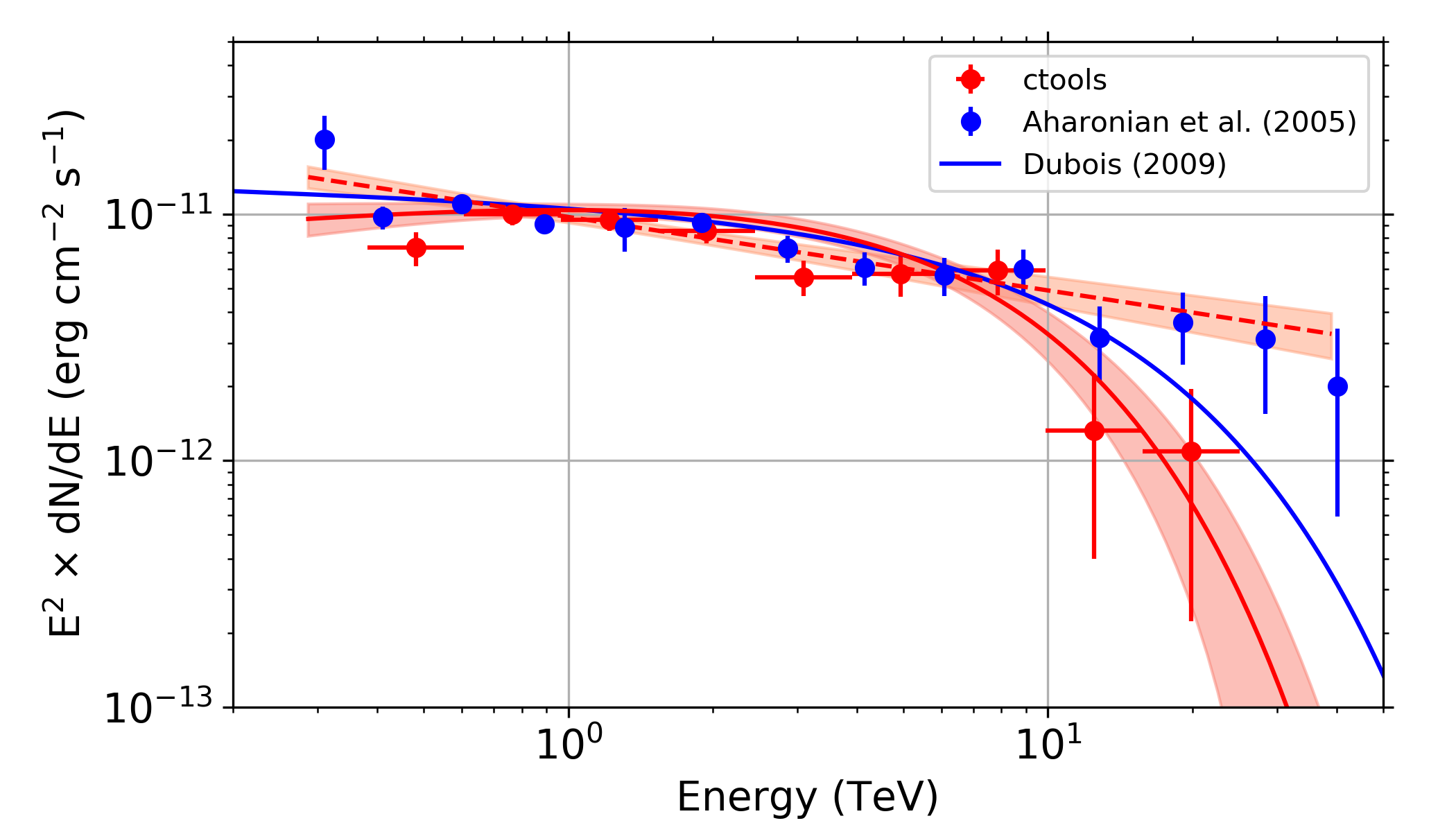
We then used csspec to derive an SED for MSH 15–52 using an unbinned maximum likelihood analysis. Spectral points were derived for ten logarithmically spaced energy bins between 381 GeV and 40 TeV. Similar to the SED generation for the Crab nebula (cf. section 2.4), the spectral energy nodes $B_{i}$ were replaced by a simple power law, and the spatial parameters $G_{\mathrm{x}}$ and $G_{\mathrm{y}}$ and the spectral power-law prefactor were fitted independently for each energy bin. The result is shown in Fig. 13, where we show for comparison also the spectral points obtained by Aharonian et al. (2005). The agreement of the spectral points between our analysis and that of Aharonian et al. (2005) is satisfactory, except for the lowest and the two highest spectral points for which we find slightly lower fluxes. Superimposed on Fig. 13 is also the spectral power-law model that we determined in the unbinned maximum likelihood fit, and the corresponding butterfly diagram generated using ctbutterfly. It turns out that the power-law spectrum clearly overestimates the flux points at low energies.

Table 5: Spectral fit results from the unbinned analysis of MSH 15–52 using an exponentially cut-off power law as spectral model.

Analysis	$k_{0}$	$\Gamma$	$E_{c}$
ctools (unbinned)	$7.7\pm 0.6$	$1.84\pm 0.13$	$5.9\pm 1.7$
Dubois (2009)	$7.1\pm 0.2$	$2.06\pm 0.05$	$11.9\pm 2.2$
HGPS catalogue	$6.9\pm 0.3$	$2.05\pm 0.06$	$19.2\pm 5.0$

Table 6: Fit results for the RX J1713.7–3946 observations under variations of the spatial model component. An exponentially cut-off power law was used for the spectral component.

Spatial model	TS	$N_{\rm src}$	R.A. (deg)	Decl. (deg)	$r$ (deg)	$w$ (deg)	$k_{0}$	$\Gamma$	$E_{c}$
H.E.S.S. published	n.c.	$\sim 31000$	-	-	-	-	$2.3\pm 0.1$	$2.06\pm 0.02$	$12.9\pm 1.1$
Disk	$681.4$	$2118$	$258.35\pm 0.01$	$-39.76\pm 0.01$	$0.52\pm 0.01$	-	$1.9\pm 0.1$	$1.94\pm 0.09$	$9.5\pm 2.9$
Gaussian	$627.7$	$2333$	$258.22\pm 0.02$	$-39.75\pm 0.02$	$0.31\pm 0.01$	-	$2.1\pm 0.2$	$2.01\pm 0.09$	$10.4\pm 3.5$
Shell	$678.0$	$2100$	$258.35\pm 0.02$	$-39.76\pm 0.01$	$0.31\pm 0.02$	$0.24\pm 0.03$	$2.0\pm 0.1$	$1.88\pm 0.10$	$7.7\pm 2.4$
Template	$762.1$	$1937$	-	-	-	-	$1.7\pm 0.1$	$1.88\pm 0.08$	$10.8\pm 2.9$
Template ($F_{x}^{0.48}$)	$784.6$	$2148$	-	-	-	-	$2.0\pm 0.1$	$1.85\pm 0.08$	$8.8\pm 2.2$

Interestingly, Dubois (2009) showed that the spectrum of MSH 15–52 deviates significantly from a simple power law, and concluded that the H.E.S.S. data are well fitted by an exponentially cut-off power law. Also in the HGPS catalogue, MSH 15–52 is fitted using an exponentially cut-off power law. Replacing the power law by an exponentially cut-off power law in our unbinned maximum likelihood analysis leads to a TS value of $780.9$ that is larger by $18.8$ with respect to the power law, corresponding to a detection of the exponential cut-off at a significance level of $4.3\sigma$. The spatial parameters found by the fit remain very close to those found for a power-law spectrum. For illustration, we superimpose the resulting spectral law together with the corresponding butterfly diagram on the spectral points in Fig. 13, where we also show for comparison the spectral law determined by Dubois (2009). The fit results for the exponentially cut-off power-law spectral model are given in Table 5 where we compare them to the values found by Dubois (2009) and the H.E.S.S. Collaboration et al. (2018). Our results are very close to those of Dubois (2009) and the H.E.S.S. Collaboration et al. (2018), although we found a slightly smaller cut-off energy compared to their analyses. Finally, we show the spatial and spectral residuals after fitting the exponentially cut-off power law in Fig. 12. The slight overestimation of the counts at low and high energies, and the underestimation in between, that we observed for the power-law spectrum in the On region (cf. Fig. 11), has now disappeared.

2.6 RX J1713.7–3946 observations

RX J1713.7–3946 is a shell-type Galactic supernova remnant and one of the largest and brightest sources of TeV gamma rays. Previous H.E.S.S. analyses (Aharonian et al. 2006b, 2007, 2011; H.E.S.S. Collaboration et al. 2018) revealed a complex emission morphology extending over about $1^{\circ}$ in diameter. To allow comparison of the ctools results with results reported in these works, we selected the energy range 300 GeV – 50 TeV for our analysis.

As a first step we focused on the modelling of the source morphology. Several extended spatial models were fitted to the data, including 2D disk, 2D Gaussian and 2D shell models as well as a spatial template map that was obtained from X-ray observations of XMM-Newton (Acero et al. 2009). Since Acero et al. (2009) suggested a non-linear flux correlation between X rays and gamma rays, we also tested modified versions of the X-ray map where all pixels were taken to a given power $\alpha$, where $\alpha=0.41$ corresponds to the value suggested by Acero et al. (2009). According to Aharonian et al. (2006b) the spectrum of RX J1713.7–3946 is curved and deviates significantly from a power law. The H.E.S.S. Collaboration et al. (2018) demonstrated that the spectrum of RX J1713.7–3946 is well described by an exponentially cut-off power law and we hence used the same spectral model in our analysis to allow comparison to that work. We used the ctlike tool to fit the source model together with the background model to the data using an unbinned maximum likelihood analysis. All spatial and spectral source parameters, as well as the parameters of the background model, were free parameters in the model fit.

The results of these model fits are summarised in Table 6. Among all tested spatial model components, the template map provides the largest statistical significance. Using the modified template maps increases the statistical significance even more, with a best fitting value of $\alpha=0.48\pm 0.10$, consistent with the value suggested by Acero et al. (2009). We find slightly smaller prefactors $k_{0}$, harder spectral indices $\Gamma$ and smaller cut-off energies $E_{c}$ compared to the H.E.S.S. Collaboration et al. (2018).

Figure 14: SED of RX J1713.7–3946 derived using csspec. Red data represent the unbinned ctools analysis, blue data are the values from Table F.1 of H.E.S.S. Collaboration et al. (2018). $68\%$ confidence level upper limits are displayed when the statistical error exceeds the value of a flux point. The red line is the fitted exponentially cut-off power-law spectral model, the light red band is the 68% confidence level uncertainty band of the spectral model and was determined using ctbutterfly. The blue line is the exponentially cut-off power-law spectral model determined by H.E.S.S. Collaboration et al. (2018).

Figure 15: Residuals after fitting the RX J1713.7–3946 observations using the $F_{x}^{0.48}$ spatial template with an exponentially cut-off power-law spectral component using an unbinned maximum likelihood fit. See Fig. 9 for a description of the panels.

Figure 16: Left: Background-subtracted counts map of the RX J1713.7–3946 observations for the energy band 300 GeV – 50 TeV. The background was estimated using the model generated by csbkgmodel with background parameters estimated using an unbinned maximum likelihood analysis using a $F_{x}^{0.48}$ spatial template with an exponentially cut-off power-law spectral component. Right: Background-subtracted sky map for the same data generated using ctskymap with the ring-background method for a correlation radius of $0.01^{\circ}$. Both maps were computed for a $0.02^{\circ}\times 0.02^{\circ}$ binning and were smoothed with a Gaussian kernel of $\sigma=0.06^{\circ}$ to reduce statistical noise. The colour bar represents the number of excess counts per $0.02^{\circ}\times 0.02^{\circ}$ bin. Coordinates are for the epoch J2000.

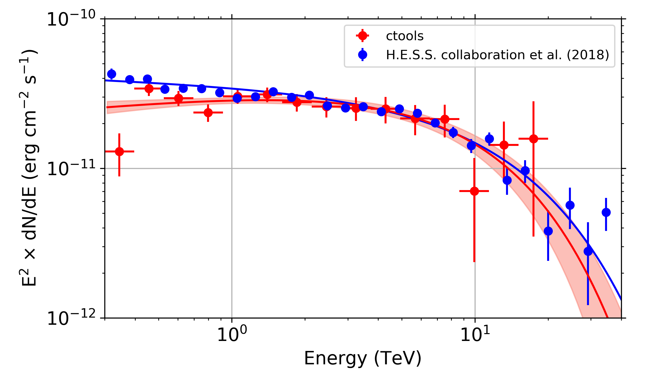
Adopting the $F_{x}^{0.48}$ spatial template we then determined the SED of RX J1713.7–3946 using csspec with an unbinned maximum likelihood analysis. We chose 15 energy bins spanning $0.3-20$ TeV for this purpose, and as before, we replaced the background model by one where $G_{\mathrm{x}}$, $G_{\mathrm{y}}$ and the spectral power-law prefactor were fitted independently for each energy bin. We also computed the butterfly diagram for the exponentially cut-off power-law spectrum using ctbutterfly, again with an unbinned maximum likelihood analysis. The results are shown in Fig. 14, which also shows the spectral points derived by the H.E.S.S. Collaboration et al. (2018) from a larger dataset. The agreement between the ctools SED and the butterfly diagram is pretty adequate, demonstrating again that the spectral results that we obtained using ctools are robust with respect to details of the background model parametrisation. The agreement between the ctools and H.E.S.S. SED is also quite satisfactory, but the ctools data point for the lowest energy ($300-397$ GeV) is significantly below the corresponding data points found by the H.E.S.S. Collaboration et al. (2018), which probably also explains why we found a flatter spectral index and smaller prefactor in our analysis. We note that this energy bin is the one that is most sensitive to imperfections in the background model because it has the smallest signal-to-background ratio, as is evidenced in the left panel of Fig. 15. This spectral point changes well beyond the statistical error for the different analysis methods considered. On the other hand, our lowest spectral point is in agreement with the Fermi-LAT analysis of RX J1713.7–3946 (cf. Fig. 5 in the H.E.S.S. Collaboration et al. 2018) and the flatter spectral index also provides a better spectral connection to the GeV data points.

The spatial and spectral residuals for the unbinned maximum likelihood fit of the $F_{x}^{0.48}$ spatial template are displayed in Fig. 15. We also examined the spectral residuals for nine spatial sub-regions, and the radial counts profiles and residuals as a function of offset angle $\theta$ for six energy bands. The corresponding plots are shown in Figs. 44 and 45 of Appendix E. For the full field of view, the spectral residuals show some significant deviations from zero below $\la 800$ GeV, but within the region of RX J1713.7–3946 the spectral residuals are relatively flat, except for two outliers near $600$ GeV and $30$ TeV. While the $30$ TeV outlier is beyond the energy range of our SED (and for which less than one event is expected from RX J1713.7–3946 in the energy bin), the SED at $600$ GeV looks rather smooth, suggesting that the outlier does not significantly impact our fitting result.

Table 7: Fit results for the RX J1713.7–3946 observations for different analysis methods. The template map scaled to $F_{x}^{0.48}$ was used as spatial model component, and an exponentially cut-off power law was used for the spectral component.

Analysis method	TS	$N_{\rm src}$	$k_{0}$	$\Gamma$	$E_{c}$
H.E.S.S. published	n.c.	$\sim 31000$	$2.3\pm 0.1$	$2.06\pm 0.02$	$12.9\pm 1.1$
Unbinned	$784.6$	$2148$	$2.0\pm 0.1$	$1.85\pm 0.08$	$8.8\pm 2.2$
Joint binned	$852.9$	$2243$	$2.1\pm 0.1$	$1.86\pm 0.08$	$9.1\pm 2.3$
Stacked binned	$806.2$	$2119$	$1.9\pm 0.1$	$1.85\pm 0.08$	$9.4\pm 2.4$
Joint On-Off (wstat)	$551.6$	$2563$	$3.2\pm 0.4$	$1.90\pm 0.15$	$4.9\pm 2.3$
Joint On-Off (wstat)	$336.5$	$1929$	$2.8\pm 0.4$	$1.51\pm 0.20$	$3.5\pm 1.3$
Joint On-Off (cstat)	$353.9$	$2034$	$2.1\pm 0.1$	$1.90\pm 0.10$	$12.3\pm 3.8$
Stacked On-Off (wstat)	$558.4$	$2612$	$2.8\pm 0.2$	$2.04\pm 0.11$	$9.0\pm 4.2$
Stacked On-Off (wstat)	$341.9$	$1977$	$2.3\pm 0.2$	$1.75\pm 0.14$	$6.9\pm 2.5$
Stacked On-Off (cstat)	$351.2$	$2009$	$2.3\pm 0.2$	$1.79\pm 0.13$	$7.9\pm 2.8$

Figure 15 demonstrates that the observed events within the source region are dominated by background events, which is different from the situation for the other three sources studied in this paper. The RX J1713.7–3946 results are thus most sensitive to inadequacies of our background model. We therefore examined the robustness of the $F_{x}^{0.48}$ spatial template fit result under variations of the background model or the analysis parameters. Specifically, we tried background models from which we remove the gradient component Eq. 2, which reduces the accuracy of the model, or where we increased the number of energy nodes, which increases the accuracy of the model but which can lead to convergence problems in the fit. We also increased the energy threshold from 300 GeV to 800 GeV. None of these modifications changed the fit result significantly, demonstrating that our result is robust with respect to analysis details.

We also note that there are some excess values in the histogram of spatial residuals that correspond to an excess feature situated in the western part of the supernova remnant, illustrating that the X-ray template does not fully describe the emission morphology of the gamma-ray emission. We note that this excess coincides with the zones 3 and 4 defined in H.E.S.S. Collaboration et al. (2018) for which the gamma-ray emission is found to reach beyond the extent of the X-ray emission. Our analysis is thus consistent with this finding.

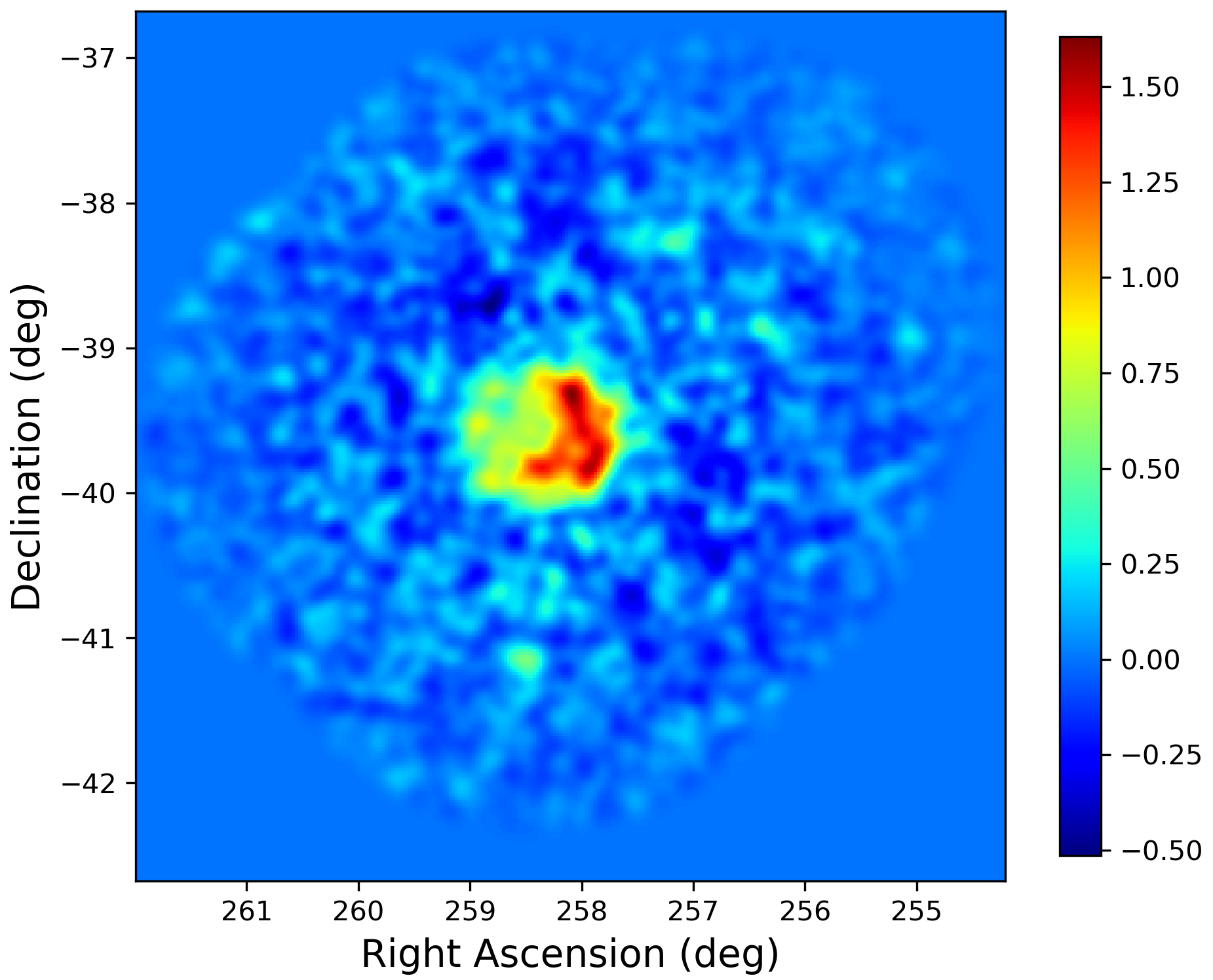
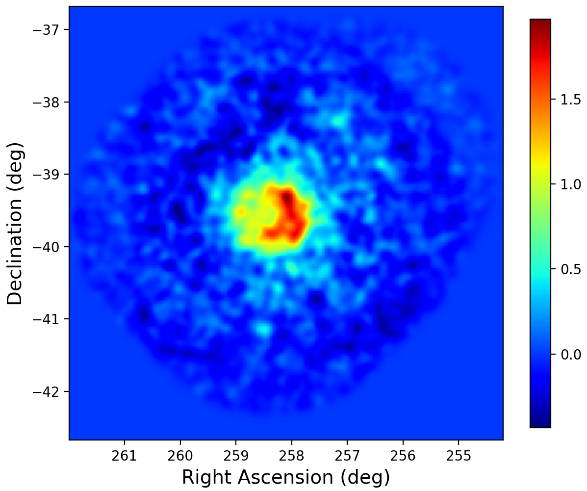
As the next step, we generated background-subtracted counts maps of the RX J1713.7–3946 observations to image the gamma-ray emission from the supernova remnant using two different methods. Firstly, the background model that was fitted to the data using the $F_{x}^{0.48}$ spatial template with an exponentially cut-off power-law spectrum was subtracted from the data, and the resulting residual map was slightly smoothed using a Gaussian kernel of $\sigma=0.06^{\circ}$. Secondly, ctskymap was used to produce a background-subtracted counts map using the so-called ring method, which estimates the background counts from a ring around the source, excluding areas where significant gamma-ray emission is detected. We selected an inner and outer ring radius of $0.8^{\circ}$ and $1^{\circ}$, respectively, and specified an exclusion region of $0.6^{\circ}$ in radius centred on Right Ascension of $258.1125^{\circ}$ and Declination of $-39.6867^{\circ}$. The correlation radius was set to $0.01^{\circ}$.

The resulting sky maps are shown in Fig. 16. The source morphologies in both maps look very similar, and also quantitatively, the number of excess counts per sky map pixel in both maps is comparable. Around the excess emission attributed to RX J1713.7–3946 the sky maps look relatively flat, and in particular, no large-scale gradients are discernable.

Finally, we compared the spectral fitting results for different analysis methods. We used again the $F_{x}^{0.48}$ spatial template together with an exponentially cut-off power law for the spectral component, and we repeated the analysis using the joint and stacked binned methods, as well as the variants of the On-Off analysis. For the binned analysis, we used spatial bins of $0.02^{\circ}\times 0.02^{\circ}$, with $200\times 200$ bins around the pointing direction of each observation for the joint analysis, and $300\times 300$ bins around Right Ascension $258.1125^{\circ}$ and Declination $-39.6867^{\circ}$ for the stacked analysis. The energy range was divided into 40 logarithmically spaced energy bins.

The same number of energy bins was also used for the On-Off analysis, and an On region of $0.6^{\circ}$ in radius centred on Right Ascension of $258.1125^{\circ}$ and Declination of $-39.6867^{\circ}$ was used. In this case we cannot use the standard implementation of the reflected-region method owing to the large size of the source, which makes impossible finding suitable reflected regions within the field of view. Therefore, the Off region was defined as a ring with inner and outer radius of $0.8^{\circ}$ and $1^{\circ}$, respectively, around the same centre as for the On region. Since this choice likely leads to different background rates per solid angle in the On and Off regions, the classical wstat analysis may lead to inaccurate results as it supposes the same background rates per solid angle in the On and Off regions. We nevertheless kept the classical wstat analysis as a reference, but also explored an alternative wstat analysis, where the scale factors $\alpha_{k,i}$ were replaced by the model-dependent scale factors $\alpha_{k,i}(M_{b})$ that were used for the cstat analysis. In that way, spatial variations of the background rates per solid angle are taken into account, but the background model is not explicitly used in the spectral analysis, and the background rates are treated as nuisance parameters based on the On and Off region counts for each energy bin (cf. Appendix C.2).

Table 7 summarises the spectral fitting results obtained with the different analysis methods. Several notable features deserve some discussion. Firstly, the 3D analyses result in larger TS values compared to the On-Off analysis, which is in line with the fact that the 3D analyses use more information to constrain the background model, leading to less statistical uncertainty on the source model. Secondly, the joint wstat analyses lead to relatively small cut-off energy values. As noted in Appendix C.2, wstat is known to be inaccurate if energy bins have zero Off counts, which is the case above $\sim 5-10$ TeV for the joint analyses of the RX J1713.7–3946 observations. Reducing the number of energy bins from 40 to 20 for the joint wstat analyses pushes the problems towards higher energies, resulting in somewhat larger cut-off energy values, steeper spectral indices and smaller prefactors. Nevertheless, even with a more severe rebinning the problem does not fully disappear, and the joint wstat results should therefore be interpreted with caution. Stacking the observations results in much larger statistics per energy bin, and the stacked results, in particular when the model-dependent scale factors $\alpha_{k,i}(M_{b})$ are used, are close to the results obtained with the 3D analyses.

Thirdly, the joint and stacked On-Off analyses using wstat result in spectral prefactors $k_{0}$ that are $40-60\%$ larger than for the unbinned analysis. This is because the estimation of the background from a ring around the supernova remnant leads to an underestimation of the background rates, since the ring is on average observed at larger offset angles than the source itself, and background rates drop with increasing offset angle. That is, the hypothesis underlying the use of wstat, which is that the background rate per solid angle is the same in the On and Off regions, is not met. Consequently, the underestimation of the background rate leads to an overestimation of the source flux. Taking the background rate variation into account using the alternative wstat analysis that uses the model-dependent scale factors $\alpha_{k,i}(M_{b})$ reduces the prefactors and makes the results more compatible with those of the unbinned analysis.

This bias can also be overcome by alternative background estimation techniques used in the publications by the H.E.S.S. Collaboration, such as the use of independent Off observations (Aharonian et al. 2007), or by applying the reflected-region method independently to several subregions within the source (H.E.S.S. Collaboration et al. 2018). This is beyond the scope of this validation study and not investigated here. We note, however, that the 3D analysis and the On-Off analysis based on cstat offer viable alternatives to obtain accurate results also for this very extended source, providing prefactors that are much closer to the values found for the unbinned analysis or published by the H.E.S.S. collaboration.

2.7 PKS 2155–304 observations

Figure 17: 68% confidence level error circles of the TeV source position derived using ctlike (red) and obtained in the H.E.S.S. analysis (Aharonian et al. 2009, blue), overlaid on over a PanSTARRS y-band image of PKS 2155–304. The white bar indicates the systematic uncertainty for H.E.S.S. localisation of $20\arcsec$ quoted in Aharonian et al. (2009). Coordinates are for the epoch J2000.

PKS 2155–304 is one of the brightest and most studied blazars in the southern hemisphere, and was first detected at TeV energies by the Durham Mark 6 telescope (Chadwick et al. 1999). PKS 2155–304 exhibits strong TeV variability, and the H.E.S.S. public data release includes observations taken during summer 2006 when the blazar was undergoing a major outburst, with ultrafast TeV flux variability at hour time scales (Aharonian et al. 2009).

Figure 18: Light curves of PKS 2155–304 derived using cslightcrv (red points) compared to the light curve obtained by the H.E.S.S. Collaboration (Aharonian et al. 2009, blue points). The ctools light curve in the top panel was derived using an unbinned maximum likelihood analysis, the one in the bottom panel using an On-Off analysis with background estimates taken from Off regions.

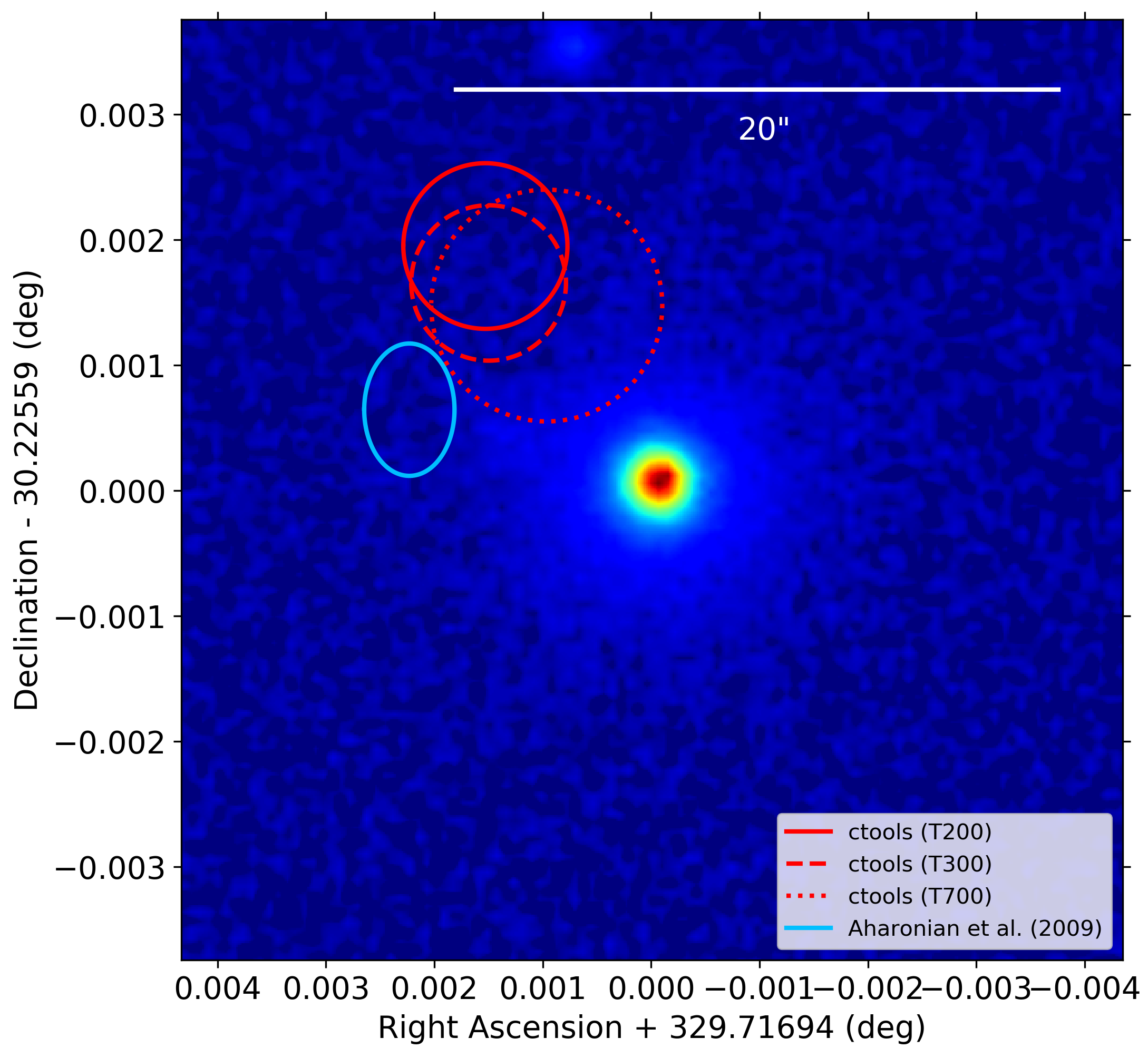
The dataset provided in the H.E.S.S. public data release corresponds to the same observations as those studied by Aharonian et al. (2009), although the event reconstruction software and background discrimination are different from those used for that paper. Aharonian et al. (2009) quote a best-fit position of the TeV source of $329.7192^{\circ}\pm 0.0004^{\circ}$ in Right Ascension and $-30.2249^{\circ}\pm 0.0005^{\circ}$ in Declination, which is $7\arcsec$ offset from the true source position at Right Ascension of $329.7169^{\circ}$ and Declination of $-30.2256^{\circ}$ (Ma et al. 1998). The systematic position uncertainty is $20\arcsec$ (Aharonian et al. 2009), considerably larger than the offset from the true source position. We performed an unbinned maximum likelihood analysis using ctlike for the datasets defined as T200, T300, and T700 in Aharonian et al. (2009) to determine the best-fitting TeV source position. The source was modelled as a point source with a curved power-law spectrum, and the background model was generated using csbkgmodel.

Figure 17 shows the results of the analysis. The best-fit ctlike source position is offset by about $5\arcsec$ from the quoted H.E.S.S. position, a distance slightly larger than the statistical location uncertainties, but considerably smaller than the systematic uncertainty of $20\arcsec$ quoted in Aharonian et al. (2009). As illustrated by the different red circles, the choice of the dataset impacts slightly the fitted source position, but within uncertainties the fitted positions are consistent. Using an exponentially cut-off power law or a curved power law as spectral component does not change the fitted source position significantly. The difference from the quoted H.E.S.S. position may be due to a difference in reconstruction software between Aharonian et al. (2009) and the H.E.S.S. public data release, as well as by a different spatial fitting technique (we used a 3D maximum likelihood fit while the H.E.S.S. results are generally obtained using a 2D technique that sums over an interval of reconstructed energies). We also note that the offset of the TeV source by $\sim 7\arcsec$ from the true source position is considerably smaller than the offset observed for the Crab nebula (see section 2.4), suggesting that the Crab nebula offset is not related to an intrinsic problem in ctools.

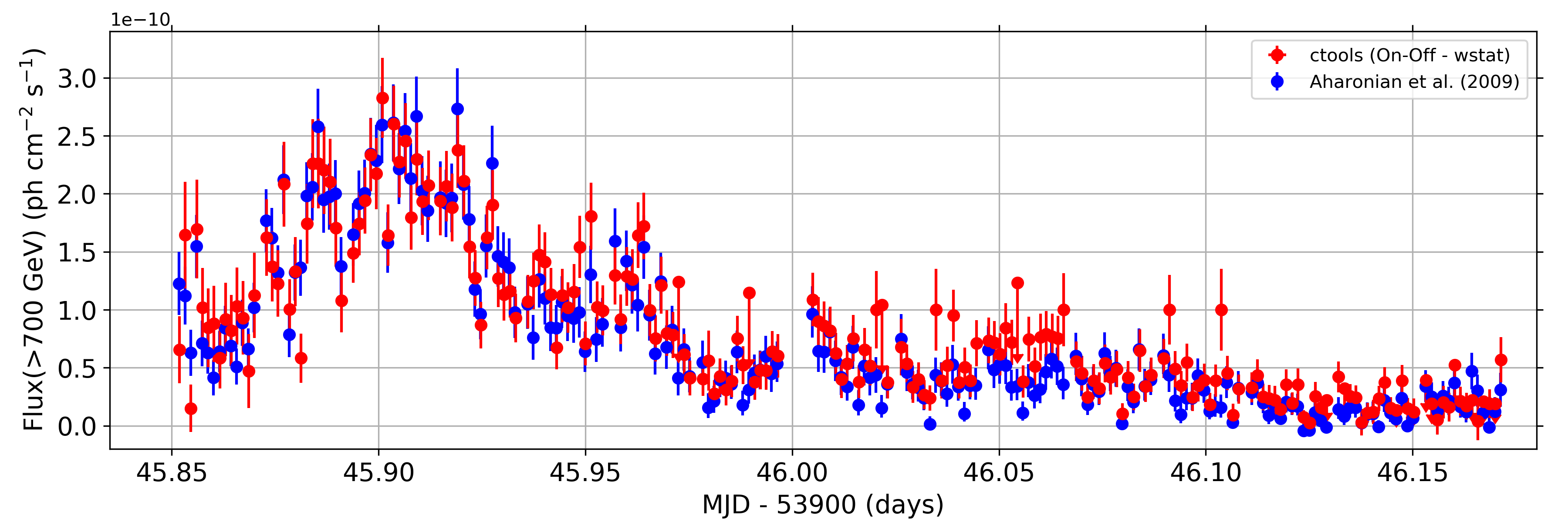
Since PKS 2155–304 is highly variable during the period covered by the H.E.S.S. flare dataset, we used cslightcrv to derive light curves of PKS 2155–304 and compared them to the one shown in Aharonian et al. (2009). In particular, we used the same time binning that was employed for Fig. 1 in Aharonian et al. (2009) and we used the event selection T700 that covers the full time interval of the observations. PKS 2155–304 was modelled as a point source, located at the true position (Right Ascension $329.7169^{\circ}$ and Declination $-30.2256^{\circ}$), with a power-law spectral component. The index of the power-law component was fixed to a fiducial value of $\Gamma=3.4$ (see below).

Figure 19: Correlation of PKS 2155–304 light curve fluxes obtained by Aharonian et al. (2009) (horizontal axis) with fluxes obtained by ctools (vertical axis). The left plot shows results for the unbinned maximum likelihood analysis, and the right plot shows results obtained for an On-Off analysis with background estimates taken from Off regions. The blue line indicates equal fluxes.

We used cslightcrv in two different modes. First, cslightcrv was run using an unbinned maximum likelihood analysis, where all events within a given $\sim 2$ minute long time interval were fitted with the source model on top of the background model. As usual, we used a background model that was generated using csbkgmodel for the unbinned analysis. Second, cslightcrv was run in On-Off mode, where events were selected from a circular On region of $0.2^{\circ}$ in radius, centred on the true source position, and the background was estimated from reflected Off regions, assuming that the background rate per solid angle in the On region is the same as in the Off regions. Consequently, the wstat statistic was used for the fitting. Ten logarithmically spaced energy bins between 700 GeV and 10 TeV were used for the On-Off analysis.

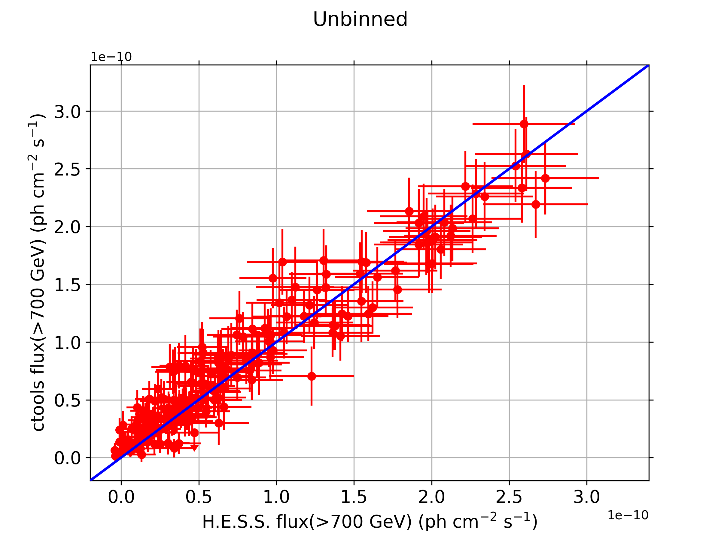
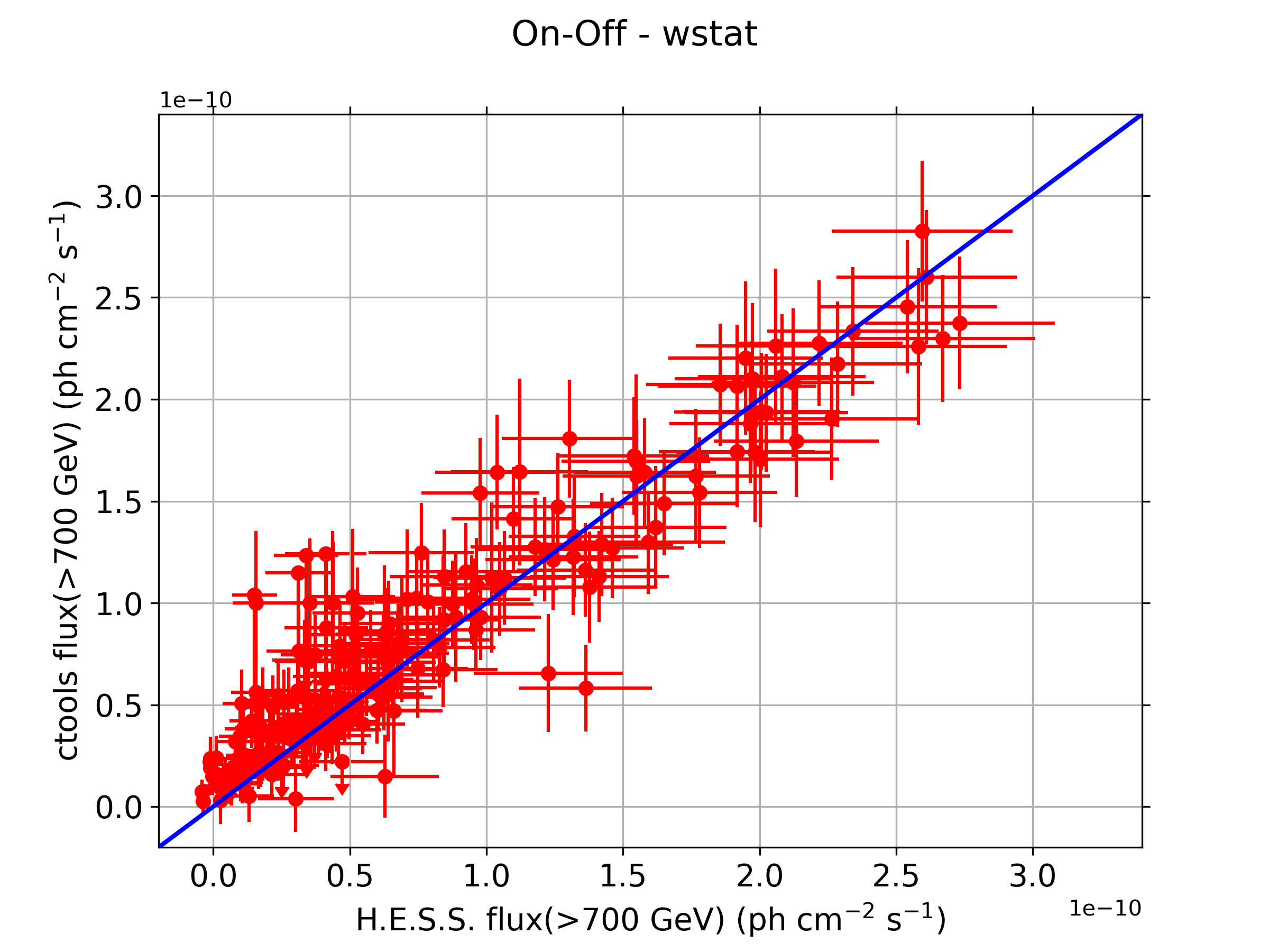
The resulting light curves are shown in Fig. 18 where they are compared to the light curve obtained by Aharonian et al. (2009) (see the bottom panel of their Fig. 1). Overall the agreement is excellent between the ctools results and the H.E.S.S. analysis. All features of the light curve obtained from the H.E.S.S. Collaboration analysis are reproduced with our ctools analyses, and our flux points overlap with the H.E.S.S. Collaboration flux points within statistical uncertainties. To demonstrate this, we show in Fig. 19 correlation plots between the ctools flux points with the flux points obtained by Aharonian et al. (2009). The flux points correlate nicely between the published H.E.S.S. and the ctools analyses, as demonstrated by the fact that the flux points intersect with the diagonal line that indicates equal flux measurements. This demonstrates that ctools enables an accurate study of the time variability of gamma-ray sources, and that the standard H.E.S.S. background model for 3D analysis, as implemented in csbkgmodel, also works satisfactorily for short, minute-long time intervals.

Figure 20: SED of PKS 2155–304 derived using csspec for the T200 dataset. Red data represent the unbinned ctools analysis, blue data are the values from Figure 9 in Aharonian et al. (2009). The red line is the fitted curved power-law spectral model, the light red band is the 68% confidence level uncertainty band of the spectral model and was determined using ctbutterfly. $68\%$ confidence level upper limits are displayed when the statistical error exceeds the value of a flux point.

Figure 21: Residuals after fitting the PKS 2155–304 observations using a point source with a curved power-law spectrum using an unbinned maximum likelihood fit. See Fig. 9 for a description of the panels.

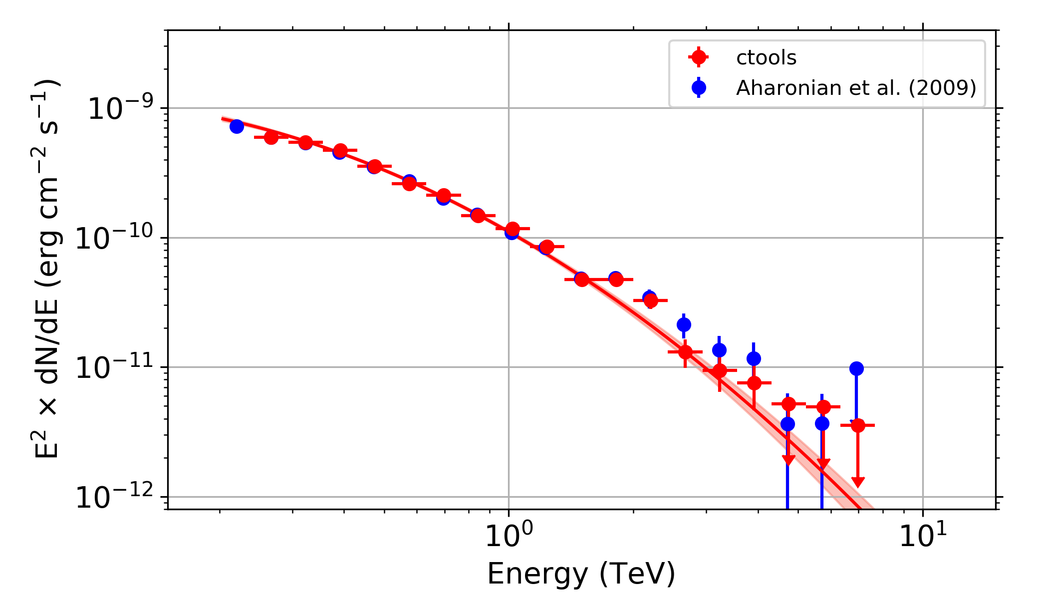
We then performed a spectral analysis of the PKS 2155–304 observations using the T200 dataset, which covers the largest energy interval. Firstly, we determined the SED of PKS 2155–304 using csspec in the usual manner by fitting the background parameters independently for each spectral point. We then derived a butterfly diagram using ctbutterfly for a power-law, an exponentially cut-off power-law, and a curved power-law spectral component using an unbinned maximum likelihood analysis. The best fit is obtained using the curved power law, followed by the exponentially cut-off power law and the power law (cf. Table 8). Figure 20 shows the SED on top of the butterfly diagram of the curved power law, superimposed on the spectrum derived by Aharonian et al. (2009) for the same dataset. Overall the agreement between the ctools analysis and the H.E.S.S. result is excellent. Only near $\sim 3$ TeV the H.E.S.S. analysis suggests slightly larger flux values, but within error bars, both SEDs are consistent.

Table 8: Fit results for PKS 2155–304 for dataset T200 under variations of the spectral model component and analysis method assuming a point-source spatial model.

PL	TS	$N_{\rm src}$	$k_{0}$	$\Gamma$		F0.3-3TeV
		counts	ph cm-2 s-1 TeV-1			erg cm-2 s-1
H.E.S.S. published	n.c.	n.c.	$(7.5\pm 0.1)\times 10^{-11}$	$3.25\pm 0.01$	-	$4.1\times 10^{-10}$
Unbinned	$46992.5$	$8922$	$(6.7\pm 0.2)\times 10^{-11}$	$3.45\pm 0.02$	-	$4.1\times 10^{-10}$
Joint binned	$43417.4$	$8116$	$(6.7\pm 0.2)\times 10^{-11}$	$3.47\pm 0.03$	-	$4.1\times 10^{-10}$
Stacked binned	$43118.4$	$8071$	$(6.5\pm 0.2)\times 10^{-11}$	$3.48\pm 0.03$	-	$4.2\times 10^{-10}$
Joint On-Off (wstat)	$17799.2$	$7877$	$(6.5\pm 0.2)\times 10^{-11}$	$3.49\pm 0.03$	-	$4.1\times 10^{-10}$
Joint On-Off (cstat)	$16244.4$	$7488$	$(6.5\pm 0.2)\times 10^{-11}$	$3.49\pm 0.03$	-	$4.1\times 10^{-10}$
Stacked On-Off (wstat)	$18366.7$	$7887$	$(6.6\pm 0.2)\times 10^{-11}$	$3.48\pm 0.03$	-	$4.1\times 10^{-10}$
Stacked On-Off (cstat)	$16866.9$	$7511$	$(6.5\pm 0.2)\times 10^{-11}$	$3.49\pm 0.03$	-	$4.1\times 10^{-10}$
EPL	TS	$N_{\rm src}$	$k_{0}$	$\Gamma$	$E_{c}$	F0.3-3TeV
		counts	ph cm-2 s-1 TeV-1		TeV	erg cm-2 s-1
H.E.S.S. published	n.c.	n.c.	$(2.1\pm 0.2)\times 10^{-10}$	$2.65\pm 0.06$	$1.0\pm 0.1$	$4.3\times 10^{-10}$
Unbinned	$47087.2$	$8902$	$(1.7\pm 0.2)\times 10^{-10}$	$2.85\pm 0.08$	$1.1\pm 0.2$	$4.2\times 10^{-10}$
Joint binned	$43507.5$	$8097$	$(1.8\pm 0.2)\times 10^{-10}$	$2.82\pm 0.08$	$1.1\pm 0.2$	$4.2\times 10^{-10}$
Stacked binned	$43197.2$	$8056$	$(1.6\pm 0.2)\times 10^{-10}$	$2.89\pm 0.08$	$1.2\pm 0.2$	$4.2\times 10^{-10}$
Joint On-Off (wstat)	$17870.4$	$7872$	$(1.6\pm 0.2)\times 10^{-10}$	$2.91\pm 0.09$	$1.2\pm 0.2$	$4.2\times 10^{-10}$
Joint On-Off (cstat)	$16321.4$	$7480$	$(1.7\pm 0.2)\times 10^{-10}$	$2.87\pm 0.09$	$1.1\pm 0.2$	$4.2\times 10^{-10}$
Stacked On-Off (wstat)	$18437.9$	$7882$	$(1.6\pm 0.2)\times 10^{-10}$	$2.90\pm 0.09$	$1.2\pm 0.2$	$4.2\times 10^{-10}$
Stacked On-Off (cstat)	$16940.7$	$7503$	$(1.7\pm 0.2)\times 10^{-10}$	$2.88\pm 0.09$	$1.2\pm 0.2$	$4.2\times 10^{-10}$
CPL	TS	$N_{\rm src}$	$k_{0}$	$\Gamma$	$\beta$	F0.3-3TeV
		counts	ph cm-2 s-1 TeV-1			erg cm-2 s-1
H.E.S.S. published	n.c.	n.c.	$(7.5\pm 0.2)\times 10^{-11}$	$3.69\pm 0.05$	$-0.78\pm 0.07$	$4.3\times 10^{-10}$
Unbinned	$47091.7$	$8900$	$(6.9\pm 0.2)\times 10^{-11}$	$3.83\pm 0.05$	$-0.35\pm 0.04$	$4.3\times 10^{-10}$
Joint binned	$43512.4$	$8097$	$(7.0\pm 0.2)\times 10^{-11}$	$3.83\pm 0.06$	$-0.37\pm 0.05$	$4.3\times 10^{-10}$
Stacked binned	$43199.5$	$8054$	$(6.8\pm 0.2)\times 10^{-11}$	$3.82\pm 0.05$	$-0.35\pm 0.05$	$4.2\times 10^{-10}$
Joint On-Off (wstat)	$17873.3$	$7877$	$(6.8\pm 0.2)\times 10^{-11}$	$3.82\pm 0.06$	$-0.34\pm 0.05$	$4.2\times 10^{-10}$
Joint On-Off (cstat)	$16322.0$	$7481$	$(6.7\pm 0.2)\times 10^{-11}$	$3.85\pm 0.06$	$-0.36\pm 0.05$	$4.2\times 10^{-10}$
Stacked On-Off (wstat)	$18442.2$	$7887$	$(6.9\pm 0.2)\times 10^{-11}$	$3.81\pm 0.06$	$-0.34\pm 0.05$	$4.2\times 10^{-10}$
Stacked On-Off (cstat)	$16944.1$	$7505$	$(6.8\pm 0.2)\times 10^{-11}$	$3.83\pm 0.06$	$-0.35\pm 0.05$	$4.2\times 10^{-10}$

Secondly, we performed ctlike model fits using a power law, an exponentially cut-off power-law, and a curved power-law spectral component for the different analysis methods available in ctools, and compared them to results given in Table 1 of Aharonian et al. (2009). For the binned analysis, we used spatial bins of $0.02^{\circ}\times 0.02^{\circ}$, with $200\times 200$ bins around the pointing direction of each observation for the joint analysis, and $250\times 250$ bins around Right Ascension $329.7169^{\circ}$ and Declination $-30.2256^{\circ}$ for the stacked analysis. The energy range was divided into 40 logarithmically spaced energy bins. The same number of energy bins was also used for the On-Off analysis. An On region of $0.2^{\circ}$ in radius centred on Right Ascension of $329.7169^{\circ}$ and Declination of $-30.2256^{\circ}$ was adopted; Off regions were defined using the reflected regions method. The results are summarised in Table 8. All spatial and spectral source parameters, as well as the parameters of the background model, were free parameters in the model fits (except for the On-Off analysis, which does not allow an adjustment of the spatial source and background parameters).

We confirm for all analysis methods that the largest TS values are obtained for a curved power law, followed by the exponentially cut-off power law and the power law. Among the different analysis methods, spectral model parameters are very close and within the statistical parameter uncertainties. With respect to the published H.E.S.S. results, the ctools results indicate a steeper spectrum and smaller spectral normalisation at 1 TeV, but the energy flux within the 300 GeV – 3 TeV energy range is comparable. A steeper ctools spectrum is consistent with the fact that the high-energy ctools spectral points are below the ones determined by Aharonian et al. (2009), as evidenced in Fig. 20. We do not know the precise origin of this difference, but it plausibly can be attributed to differences in the analysis details or reconstruction methods used.

Finally, the spatial and spectral residuals for the unbinned maximum likelihood fit of the curved power law spectrum are displayed in Fig. 21. Spectral residuals for nine sub-sectors and radial counts profiles and residuals as a function of offset angle $\theta$ are shown in Figs. 46 and 47 of Appendix E. The spectral residuals are relatively flat, yet the significance distribution of the residual counts shows some positive excess values, and residual features around PKS 2155–304 are also visible in the residual map. These features are probably attributable to the strong variability of the source, which is not properly taken into account for the spectral and residual analyses that assume a constant source flux. In general, the point-spread function will vary in time, as a consequence of the changing zenith angle of the pointing direction during the observation period. For the PKS 2155–304 observations, the zenith angle changed between $7.2^{\circ}$ and $27.1^{\circ}$, resulting in a variation of the $68\%$ containment radius at 1 TeV and an offset angle of $0.5^{\circ}$ between $4.7^{\prime}$ and $5.4^{\prime}$, respectively. Assuming a constant source flux will give equal weight to the point-spread function of each observation, while for a varying source flux, the observations during which the source flares will have greater weight. It is hence not surprising that some spatial residuals remain, which are mainly situated at the edge of the field of view and hence should not significantly affect the results for the source. In addition, the excess values seen in Fig. 21 are relatively modest.

3 Joint analysis of H.E.S.S. and Fermi-LAT data

Figure 22: Left: SED of the Crab nebula derived from the joint analysis of Fermi-LAT and H.E.S.S. data above 50 GeV. H.E.S.S. data were analysed using two different methods, unbinned and On-Off with wstat statistics (see Section 2.4). Lines represent the best-fit curved power-law spectral models over the entire energy range, and the shaded bands represent the 68% confidence-level uncertainty bands of the spectral models determined using ctbutterfly. Upper limits from the On-Off analysis at the highest energies are above the maximum flux shown in the plot. Right: Best-fit curved power-law model and SED derived from our joint analysis of LAT and H.E.S.S. data (with unbinned analysis of H.E.S.S. data), compared to published results from H.E.S.S. only (Aharonian et al. 2006a), Fermi-LAT only above 50 GeV (Ackermann et al. 2016), and MAGIC (Aleksić et al. 2015).

The ctools also are capable of analysing IACT data jointly with data from other gamma-ray instruments. The H.E.S.S. public data release enables testing this feature for the first time with real IACT data. Here we illustrate, as a test case, a joint spectral analysis of the Crab nebula using H.E.S.S. observations (Section 2.4) along with data from the Fermi Large Area Telescope (LAT, Atwood et al. 2009).

3.1 Preparation of Fermi-LAT data

The Fermi LAT is a space-borne pair-tracking gamma-ray imaging telescope detecting photons in the energy range from 20 MeV to greater than 1 TeV. It has been operating since 2008 and its data are publicly available. For this analysis we retrieved all candidate photon events measured with the LAT over about 124 months from the beginning of the scientific operations (MET from 239 557 417 s to 565 315 205 s), in a circle centred at Right Ascension of $83.633^{\circ}$, Declination of $22.015^{\circ}$, and a radius of $2.3^{\circ}$, and belonging to the P8R3 SOURCE event class (Atwood et al. 2013; Bruel et al. 2018).

We prepared the LAT data using fermitools 1.0.1 and used the P8R3_SOURCE_V2 instrument response functions. We selected candidate photons with energies between 50 GeV and 1 TeV. The lower energy limit is chosen to avoid complications in accounting for the Crab pulsar. Based on the spectra measured in Ansoldi et al. (2016), the contribution of the pulsar above 50 GeV is $\lesssim 4\%$ with respect to the nebula; thus the pulsar can be neglected for the purpose of this validation study. An accurate determination of the nebula spectrum at lower energies can be obtained by using an event selection based on the pulsar phase. However, this is beyond the scope of this paper and not investigated here. The upper energy limit follows the standard recommendations for the analysis of LAT data. We also selected events with measured arrival directions $<105^{\circ}$ from the local zenith to reduce the contamination from the bright gamma-ray emission from the Earth’s atmosphere.

We used gtbin to bin the events in measured arrival direction and energy. For the arrival direction we used a $3^{\circ}\times 3^{\circ}$ region centred at Right Ascension $83.633^{\circ}$, Declination $22.015^{\circ}$, and with a grid step of $0.05^{\circ}$ in Plate Carrée (CAR) projection in celestial coordinates. For the energy binning we used 15 logarithmically spaced bins between 50 GeV and 1 TeV. We combined together all LAT event types (with different PSF and energy-dispersion qualities). It would be possible to treat event types separately using a joint likelihood in the following ctlike analysis, but this is not investigated here. We calculated the LAT live time as a function of direction in the sky and incidence angle with respect to the LAT boresight using gtltcube. We computed the exposure using gtexpcube2 over the analysis region, plus a $3^{\circ}$ border to ensure a proper convolution of the models with the PSF. Finally we used gtsrcmaps to calculate the spatial convolution with the LAT PSF of the standard LAT models for the diffuse backgrounds, namely interstellar emission from the Milky Way (gll_iem_v07.fits) and the isotropic background (iso_P8R3_SOURCE_V2_v1.txt). A model for the Crab nebula was not included in this step: the source of interest will be modelled directly in ctlike as described in the next paragraph.

Table 9: Best-fit spectral parameters of the Crab nebula at energies $>50$ GeV from the joint fit to the Fermi-LAT and H.E.S.S. data compared to results from MAGIC (Aleksić et al. 2015) and from the joint analysis of LAT, MAGIC, VERITAS, FACT, and H.E.S.S. (Nigro et al. 2019). The spectrum is modelled using a curved power law $dN/dE(E)=k_{0}(E/E_{0})^{-\Gamma+\beta\ln(E/E_{0})}$ with a pivot energy $E_{0}=1$ TeV. $k_{0}$ is given in units of $10^{-11}$ cm^-2 s^-1 TeV^-1.

	$k_{0}$	$\Gamma$	$\beta$
LAT (binned) + H.E.S.S. (unbinned)	$4.6\pm 0.2$	$2.43\pm 0.03$	$-0.115\pm 0.016$
LAT (binned) + H.E.S.S. (stacked On-Off wstat)	$4.5\pm 0.2$	$2.42\pm 0.04$	$-0.111\pm 0.018$
LAT (binned) + H.E.S.S. (unbinned, response scale)	$4.3\pm 0.5$	$2.45\pm 0.05$	$-0.113\pm 0.017$
LAT (binned) + H.E.S.S. (stacked On-Off wstat, response scale)	$4.3\pm 0.5$	$2.43\pm 0.05$	$-0.110\pm 0.018$
MAGIC	$3.23\pm 0.03$	$2.47\pm 0.01$	$-0.104\pm 0.004$
LAT + MAGIC + VERITAS + FACT + H.E.S.S.	$3.85\pm 0.11$	$2.51\pm 0.03$	$-0.104\pm 0.009$

3.2 Spectrum of the Crab nebula from Fermi-LAT and H.E.S.S. data

We used ctlike to perform a joint fit of the LAT data, prepared as described in the previous section, along with H.E.S.S. data treated as described in Section 2.4. We note that for LAT data ctlike at present does not account for energy dispersion. We chose only two methods to analyse H.E.S.S. data here as two extreme representative cases, namely the unbinned analysis and the stacked On-Off analysis with wstat statistic. We modelled the spectrum of the Crab nebula as a curved power law, $dN/dE(E)=k_{0}(E/E_{0})^{-\Gamma+\beta\ln(E/E_{0})}$, with a pivot energy $E_{0}=1$ TeV, to compare with the best fit to MAGIC data above 50 GeV presented in Aleksić et al. (2015). For LAT data we included in the likelihood analysis the models for the diffuse backgrounds described in the previous section. Owing to the limited size of the analysis region and low counting statistics we fixed the normalisation of the isotropic background template to one, and we left as free parameter only the normalisation of the Galactic interstellar model. For the latter we verified that the fitted normalisation is always compatible within statistical uncertainties with one. Diffuse gamma-ray emission can be ignored in the analysis of H.E.S.S. data because its intensities are expected to be small with respect to the residual cosmic-ray background and the Crab nebula itself owing to the higher energy threshold. Conversely, for H.E.S.S. we included the model previously described for the residual cosmic-ray background in the unbinned analysis. In the analysed region, no other gamma-ray sources are detected above 10 GeV (Ajello et al. 2017).

A general validation of ctools for the analysis of LAT data has not been performed yet. It is beyond the scope of this paper, and left for future work. Nevertheless, we have verified that if we analyse the LAT dataset alone by using ctlike the best-fit parameter values and errors are in excellent agreement with the results obtained using gtlike (the likelihood tool of the fermitools suite).

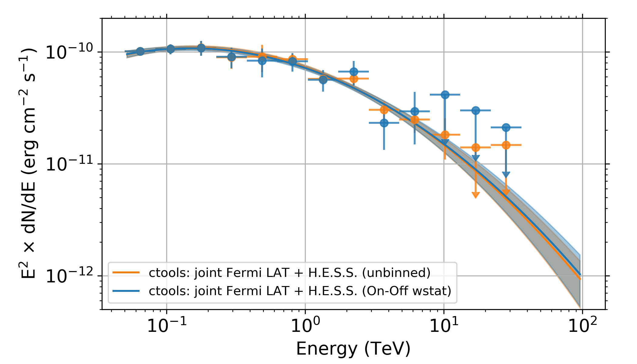
Table 9 summarises the results from the two different analyses of the LAT and H.E.S.S. data, which are in excellent agreement. Specifically, the second analysis, that is a binned analysis for the LAT and a stacked On-Off wstat analysis for H.E.S.S., corresponds to the well-established standard analysis method for each instrument, and gives comparable results as a binned analysis for the LAT combined with an unbinned analysis for H.E.S.S.. We have thus demonstrated that the unbinned analysis for H.E.S.S. data can be effectively used in joint analyses as well. We have also shown that it is possible to combine analysis techniques tailored to each instrument in a joint analysis, going beyond the approach illustrated in Nigro et al. (2019) that analyse LAT data by unconventionally using the On-Off method to match the standard approach for IACT data.

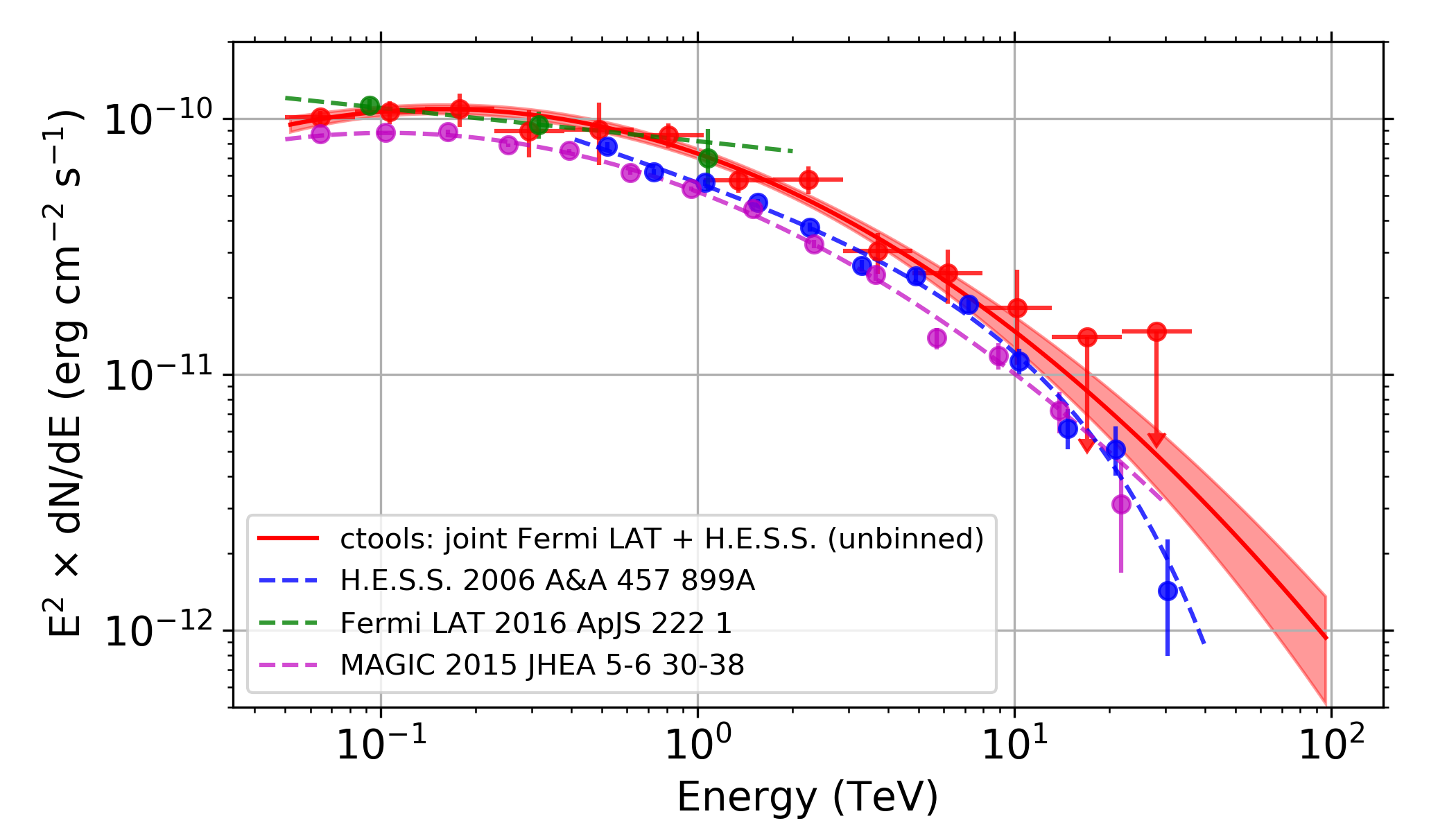
The spectral parameters $\Gamma$ and $\beta$ are in good agreement with the results obtained from the independent observations with MAGIC over an equivalent energy range $>50$ GeV (Aleksić et al. 2015), and from the joint analysis of LAT, MAGIC, VERITAS, FACT, and H.E.S.S. data in Nigro et al. (2019). The normalisation $k_{0}$ from our analysis is larger by 30% than what was reported by MAGIC, that, given the completely different datasets, is reasonably consistent with systematics related to flux measurements by IACT telescopes (see for example the discussion on flux systematics in H.E.S.S. Collaboration et al. 2018, or the variations between values of $k_{0}$ from different instruments in Nigro et al. 2019).

We then used csspec to derive the SED of the Crab nebula over 15 bins in energy from 50 GeV to 100 TeV. The resulting SEDs are shown in Figure 22. The SEDs show once again that there is an excellent agreement between results obtained using the unbinned and On-Off analysis of H.E.S.S. data in this case. The findings are also consistent with published results (Aharonian et al. 2006a; Aleksić et al. 2015; Ackermann et al. 2016). We note that the higher fluxes found in our analysis compared to Aleksić et al. (2015) are also inferred from Fermi-LAT data alone below 2 TeV in Ackermann et al. (2016).

We checked for differences in the absolute flux level between H.E.S.S. and the LAT. On one hand, the relevant systematic uncertainties for the LAT are the uncertainties in the effective area, that for our dataset without accounting for energy dispersion amount to 5% between 50 GeV and 100 GeV, and then increase linearly as a function of logarithm of energy to reach 15% at 1 TeV, and the uncertainties in the absolute energy scale, that amount to $-3.0\%\pm 0.4\%\,(\mathrm{statistical})\pm 2.0\%\,(\mathrm{systematic})$ (Abdollahi et al. 2017). On the other hand, for H.E.S.S. the systematic uncertainties in the flux measurement are 30% (H.E.S.S. Collaboration et al. 2018). Therefore, for simplicity, we neglected the smaller uncertainties for the LAT, that is we fixed the LAT effective area to nominal, and we introduced for H.E.S.S. a scaling factor that multiplies the effective area. We included the scale parameter as an additional free parameter in the fit to the data, and we found that the best-fit values are $1.09\pm 0.16$ for the unbinned analysis, and $1.04\pm 0.15$ for the wstat analysis, respectively. Therefore, the absolute flux levels measured by the LAT and H.E.S.S. are consistent within statistical uncertainties for the datasets and models considered. The scale factors obtained are well within the level of systematic uncertainties reported for the two instruments. In Table 9 we show the analysis results also for the case with the scale factor as free parameter: all the parameter values are in good agreement with those obtained without applying the response scaling. We note that with the effective area scaling factor as a free parameter the uncertainty in the prefactor $k_{0}$ is significantly increased due to the degeneracy between the two parameters, or, in other words, due to the fact that once a free scaling factor is introduced for H.E.S.S. the constraints on the normalisation are provided by LAT data alone.

4 Conclusion

We presented a comprehensive analysis of the first public H.E.S.S. data release observations using the ctools astronomical gamma-ray data analysis software package version 1.6. We introduced a parametrised background model that describes the expected number of background events as a function of energy and position in the field of view for each observation. The background model was defined and validated using the empty-field observations that are included in the H.E.S.S. data release.

We used this model to derive analysis results for the Crab nebula, MSH 15–52, RX J1713.7–3946, and PKS 2155–304. Results were obtained using the different analysis methods available in ctools, including binned and unbinned 3D maximum-likelihood methods, and several variants of the classical On-Off techniques. The achieved results were consistent among these different analysis methods. We compared our results to equivalent H.E.S.S. results reported in literature that were obtained by the H.E.S.S. Collaboration using their internal software. Overall we found a favourable agreement with the published H.E.S.S. results. A detailed quantitative comparison is however not possible, since, in general, the published H.E.S.S. results are based on larger datasets than those included in the public H.E.S.S. data release, and the H.E.S.S.-internal processing software version used for the publications also differs from the software version used for the public H.E.S.S. data release.

This was the first validation of ctools on real Imaging Atmospheric Cherenkov Telescope data, and to our knowledge, this work is the first successful application of an unbinned 3D maximum likelihood analysis to extract the characteristics of gamma-ray sources from such data. This validation represents an important milestone, as it paves the way towards a broader use of ctools for Imaging Atmospheric Cherenkov Telescope data analysis, and towards its future application to data from the Cherenkov Telescope Array. Likely, the parametrised background model used in this work is too simplistic and needs refinement, in particular for the application of ctools to CTA data. Yet there is in principle no obstacle to defining more complex models that reliably represent the distribution of the background events in the data. In this paper we made the proof of principle, and we are confident that this principle also holds for more complex situations.

Finally, we also demonstrated that ctools readily enables a broad-band multi-instrument data analysis by combining and jointly analysing public data from the two different instruments Fermi-LAT and H.E.S.S. to constrain spectral models. Such a multi-instrument analysis is fundamental for understanding gamma-ray sources, since emission spectra from a single physical process typically span several orders of magnitude in energy. Consequently, broad-band studies are needed to discriminate between emission processes and to constrain the physical properties of the underlying particle populations. And with the upcoming CTA, such joint studies will probably be needed to disentangle and study the emission from the many sources that will often spatially overlap along the line of sight in the inner regions of our Galaxy.

Appendix A Residuals computation

We express residuals throughout this paper as significance in units of Gaussian $\sigma$, computed using a log-likelihood-ratio test for Poisson statistics. The two hypotheses in the test are that the model is sufficient to describe the data (null hypothesis) with log-likelihood given by

$$\ln L_{0}=\exp{(-m)}\,\frac{m^{n}}{n!},$$ (7)

where $n$ is the number of observed counts, and $m$ the number of expected counts based on the model, or that the data comprise the model plus an unknown residual component (alternative hypothesis), the sum of which is assumed to match the observed number of counts $n$, so that the log-likelihood is

$$\ln L_{\rm test}=\exp{(-n)}\,\frac{n^{n}}{n!}.$$ (8)

Based on Wilks’ theorem (Wilks 1938) twice the logarithm of the likelihood ratio is distributed as a $\chi^{2}$ with one degree of freedom (for one additional parameter, the unknown number of residual counts set to match the data), and, therefore, its square root is distributed as a normal variable. The final formula for the residual $r$ expressed as significance in Gaussian $\sigma$ is

$$r=\operatorname{sgn}(n-m)\sqrt{2\left(n\ln\frac{n}{m}+m-n\right)},$$ (9)

where the sign term indicates whether the measured number of counts is larger or smaller than the number of counts predicted by the model. Some special cases need to be treated separately. Namely, if $n=0$ the residual significance is

$$r=\operatorname{sgn}(n-m)\sqrt{2m},$$ (10)

while if $m=0$ the significance cannot be computed and we set $r=0$. This implies that the method becomes inaccurate in the low-counting regime. The residual computation is implemented in the csresmap and csresspec scripts.

Appendix B Maximum likelihood estimation

The central method behind the ctools data analysis is the maximum likelihood estimation of the parameters of a given model. The method obtains the parameter estimates by finding the parameter values that maximise the likelihood function $L(M)$. The likelihood function quantifies the probability that the data are drawn from a particular model $M$. The formula used for the likelihood depends on whether the data are unbinned or binned and on the assumed underlying statistical law. For the 3D analyses, the reader should refer to Knödlseder et al. (2016b) for the likelihood formulae; for the On-Off analyses they are given in Appendix C.2.

We used an iterative Levenberg-Marquardt algorithm for the estimation of the maximum of the likelihood function $L(M)$. Since the Levenberg-Marquardt algorithm minimises a function, $-\ln L(M)$ is used as the function to minimise. The Levenberg-Marquardt algorithm starts with an initial guess of the model parameters $a_{k}$ and iteratively replaces this estimate by a new estimate $a_{k}+\Delta a_{k}$. The $\Delta a_{k}$ are determined by solving

$$\sum_{l}\alpha_{kl}(1+\delta_{kl}\lambda)\Delta a_{l}=\beta_{k},$$ (11)

where

$$\alpha_{kl}=\frac{\partial^{2}(-\ln L(M))}{\partial a_{k}\partial a_{l}}$$ (12)

is the curvature matrix,

$$\beta_{k}=\frac{\partial(-\ln L(M))}{\partial a_{k}}$$ (13)

is the gradient, and $\delta_{kl}$ is the Kronecker delta that is $1$ for $k=l$ and $0$ otherwise. $\lambda$ is a damping parameter that initially is set to $0.001$. If a Levenberg-Marquardt iteration leads to an increase of the log-likelihood function $\ln L(M)$, $\lambda$ is decreased by a factor of 10. If the log-likelihood function $\ln L(M)$ does not improve, $\lambda$ is increased by a factor of 10 and the iteration is repeated. The iterations are stopped when the log-likelihood increase is less than a small value, typically $0.005$; the optimiser status is then set to converged. The iterations are also stopped if the log-likelihood function does not increase for (typically) ten iterations; the optimiser status is then set to stalled.

The matrix equation is solved using a sparse matrix Cholesky decomposition. Parameters are constrained within their parameter limits in case they have been specified by the user. Gradients for background model parameters are computed analytically. If energy dispersion is neglected (option edisp=no), gradients for spectral source model parameters are also computed analytically. Otherwise, analytical computation is not possible, and gradients are computed numerically using a two-point formula. Numerical gradients are also used for spatial source model parameters.

Statistical errors on the model parameters $\delta a_{k}$ are determined by computing the square root of the diagonal elements of the covariance matrix $C$ which is the inverse of the curvature matrix:

$$\delta a_{k}=\sqrt{C_{kk}}$$ (14)

with

$$C=[\alpha]^{-1}.$$ (15)

Inversion of $[\alpha]$ is again performed using a sparse matrix Cholesky decomposition. Maximum-likelihood estimation is implemented by ctlike.

If gamma-ray emission from a source is not detected, an upper limit for the flux can be derived by determining the flux $F_{\mathrm{up}}$ that leads to a log-likelihood decrease of $\Delta\ln L$ with respect to the maximum log-likelihood estimate $F_{\mathrm{0}}$:

$$\ln L(F_{\mathrm{up}})=\ln L(F_{\mathrm{0}})-\Delta\ln L.$$ (16)

The log-likelihood decrease $\Delta\ln L$ is computed from the chance probability (p-value) using

$$\Delta\ln L=(\mathrm{erf}^{-1}(p))^{2}.$$ (17)

Upper limit computation is implemented by ctulimit.

Appendix C On-Off spectral analysis

C.1 On-Off spectra and response

The data for the On-Off spectral analysis were prepared using the csphagen script which generates the necessary files from one or several event lists in the OGIP format normally used in X-ray astronomy. This format is composed of Pulse Height Analyser spectral files (PHA), an Auxiliary Response File (ARF) and a Redistribution Matrix File (RMF).

Data were either analysed in joint or stacked mode. In joint mode, PHA, ARF, and RMF files are generated for each observation $i$. PHA files are generated for the On and Off regions by binning the events in both regions for each observation $i$ as a function of reconstructed energy $k$, resulting in vectors $n^{\mathrm{on}}_{k,i}$ and $n^{\mathrm{off}}_{k,i}$, respectively. The ARF is given by

$$ARF_{i}(E)=\int_{\mathrm{on}}\int_{\@vec{p}}A_{\rm eff}(\@vec{p},E)\times PSF(\@vec{p^{\prime}}|\@vec{p},E)\times M_{s}(\@vec{p},E)\,d\@vec{p}\,d\@vec{p^{\prime}},$$ (18)

where $A_{\rm eff}(\@vec{p},E)$ is the effective area, $PSF(\@vec{p^{\prime}}|\@vec{p},E)$ is the point-spread function, $M_{s}(\@vec{p},E)$ is the source model, $\@vec{p}$ and $\@vec{p^{\prime}}$ are the true and reconstructed photon arrival directions, respectively, and $E$ is the true energy (see Knödlseder et al. (2016b) for the definition of the terms). The integration in $\@vec{p^{\prime}}$ is done over the On region, and the integration in $\@vec{p}$ is done over all $\@vec{p}$ that contribute events within the On region. In practice, the ARF is stored as a vector for a specified number of true energies. The RMF is given by

$$RMF_{k,i}(E)=\frac{\int_{\mathrm{on}}\int_{E^{\prime}_{k}}A_{\rm eff}(\@vec{p},E)\times E_{\rm disp}(E^{\prime}|\@vec{p},E)\,dE^{\prime}\,d\@vec{p}}{\int_{\mathrm{on}}A_{\rm eff}(\@vec{p},E)\,d\@vec{p}},$$ (19)

where $E_{\rm disp}(E^{\prime}|\@vec{p},E)$ is the energy dispersion. The integration in $\@vec{p}$ is done over the On region to allow for possible variations of the energy dispersion over that region, but given the typically small size of the On region we can approximate

$$RMF_{k,i}(E)\approx\int_{\mathrm{on}}\int_{E^{\prime}_{k}}E_{\rm disp}(E^{\prime}|\@vec{p},E)\,dE^{\prime}\,d\@vec{p}.$$ (20)

The integration over reconstructed energy $E^{\prime}$ is done over the width of the energy bin $k$.

csphagen also computes the background scaling factors $\alpha_{k,i}$ that are stored in the BACKSCAL column of each On PHA file, and background response vectors $b_{k,i}$ that are stored in the BACKRESP column of each Off PHA file. The background scaling factors are computed using

$$\alpha_{k,i}=\frac{\int_{\mathrm{on}}M_{b}(\@vec{p^{\prime}},E^{\prime})\,d\@vec{p^{\prime}}}{\int_{\mathrm{off}}M_{b}(\@vec{p^{\prime}},E^{\prime})\,d\@vec{p^{\prime}}},$$ (21)

where $M_{b}(\@vec{p^{\prime}},E^{\prime})$ is a background acceptance model, specified either using a model definition XML file, or the template background found in the IRF. If no background acceptance model is provided, $M_{b}(\@vec{p^{\prime}},E^{\prime})=1$, and $\alpha_{k,i}$ gives the solid angle ratio between On and Off regions. The background response vectors are computed using

$$b_{k,i}=\int_{\mathrm{off}}M_{b}(\@vec{p^{\prime}},E^{\prime})\,d\@vec{p^{\prime}},$$ (22)

where $M_{b}(\@vec{p^{\prime}},E^{\prime})$ are evaluated at the reconstructed energy bins $k$. If no background acceptance model is provided, $M_{b}(\@vec{p^{\prime}},E^{\prime})=1$, and $b_{k,i}$ gives the solid angle of the Off region.

In stacked mode, events from all observations $i$ are combined into a single On and Off PHA spectrum and the effective response functions are computed using

$$n^{\mathrm{on}}_{k}=\sum_{i}n^{\mathrm{on}}_{k,i}$$ (23)

$$n^{\mathrm{off}}_{k}=\sum_{i}n^{\mathrm{off}}_{k,i}$$ (24)

$$ARF(E)=\frac{\sum_{i}ARF_{i}(E)\times\tau_{i}}{\sum_{i}\tau_{i}}$$ (25)

$$RMF_{k}(E)=\frac{\sum_{i}RMF_{k,i}(E)\times ARF_{i}(E)\times\tau_{i}}{\sum_{i}ARF_{i}(E)\times\tau_{i}}$$ (26)

$$\alpha_{k}=\frac{\sum_{i}\alpha_{k,i}\times b_{k,i}\times\tau_{i}}{\sum_{i}b_{k,i}\times\tau_{i}}$$ (27)

$$b_{k}=\frac{\sum_{i}b_{k,i}\times\tau_{i}}{\sum_{i}\tau_{i}},$$ (28)

where $\tau_{i}$ is the live time (or exposure) of observation $i$.

C.2 Likelihood for On-Off spectral analysis

On-Off data were analysed using the maximum likelihood method (see Appendix B). For energy-binned On-Off data following the Poisson distribution the log-likelihood function $L_{i}(M)$ can be expressed as

$$-\ln L_{i}(M)=\sum_{k}m^{\mathrm{on}}_{k,i}(M)-n^{\mathrm{on}}_{k,i}\ln m^{\mathrm{on}}_{k,i}(M)+m^{\mathrm{off}}_{k,i}(M)-n^{\mathrm{off}}_{k,i}\ln m^{\mathrm{off}}_{k,i}(M),$$ (29)

where the sum is performed over energy bins $k$, $n^{\mathrm{on}}_{k,i}$ and $n^{\mathrm{off}}_{k,i}$ are the number of events observed in the On and Off regions, for energy bin $k$ and observation $i$, respectively, and $m^{\mathrm{on}}_{k,i}$ and $m^{\mathrm{off}}_{k,i}$ are the numbers of events expected in these bins based on the model $M$ in the On and Off regions, respectively.

It is convenient to split the model in signal (gamma rays) and background, $M=M_{s}+M_{b}$. Let $\alpha_{k,i}(M_{b})$ be the scale factor that transforms the number of expected background counts in the Off region into the number of expected background counts in the On region. The log-likelihood in Equation 29 can then be reformulated as

$$\begin{split}-\ln L_{i}(M)=\sum_{k}&s_{k,i}(M_{s})+\alpha_{k,i}(M_{b})\,b_{k,i}(M_{b})-\\ &n^{\mathrm{on}}_{k,i}\ln[s_{k,i}(M_{s})+\alpha_{k,i}(M_{b})\,b_{k,i}(M_{b})]+\\ &b_{k,i}(M_{b})-n^{\mathrm{off}}_{k,i}\ln b_{k,i}(M_{b}),\end{split}$$ (30)

where $s_{k,i}(M_{s})$ is the number of expected signal counts in the On region, and $b_{k,i}(M_{b})$ is the number of expected background counts in the Off region of energy bin $k$ and observation $i$. For consistency with XSPEC this statistic is called cstat.

In practice a background model is not always available. The likelihood can be reformulated in this case by adopting as single assumption that the background rates per unit solid angle and background spectrum are the same in the On and Off regions (this matches the general expectations for reflected Off regions, which is the main On-Off method implemented in ctools). Thus, the factors $\alpha_{k,i}$ can be calculated as the ratio of solid angle subtended by the On region over that subtended by the Off region. Furthermore, the terms $b_{k,i}$ can be treated as nuisance parameters that is derived by solving the equations

$$\frac{\partial\ln L}{\partial b_{k,i}}=0.$$ (31)

This yields quadratic equations for $b_{k,i}$

$$1+\alpha_{k,i}-\frac{\alpha_{k,i}\,n^{\mathrm{on}}_{k,i}}{s_{k,i}(M_{s})+\alpha_{k,i}b_{k,i}}-\frac{n^{\mathrm{off}}_{k,i}}{b_{k,i}}=0$$ (32)

which have the general solution

$$b_{k,i}(M_{s})=\frac{C_{k,i}(M_{s})+D_{k,i}(M_{s})}{2\alpha_{k,i}(\alpha_{k,i}+1)},$$ (33)

where

$$C_{k,i}(M_{s})=\alpha_{k,i}(n^{\mathrm{on}}_{k,i}+n^{\mathrm{off}}_{k,i})-(\alpha_{k,i}+1)s_{k,i}(M_{s}),$$ (34)

and

$$D_{k,i}(M_{s})=\sqrt{C^{2}_{k,i}(M_{s})+4\alpha_{k,i}(\alpha_{k,i}+1)\,n^{\mathrm{off}}_{k,i}\,s_{k,i}(M_{s})}.$$ (35)

By replacing the values of $b_{k,i}$ obtained from Eq. 33 in Eq. 30 one obtains a formulation of the log-likelihood that depends only on $M_{s}$:

$$\begin{split}-\ln L_{i}(M_{s})=\sum_{k}&s_{k,i}(M_{s})+\alpha_{k,i}b_{k,i}(M_{s})-\\ &n^{\mathrm{on}}_{k,i}\ln[s_{k,i}(M_{s})+\alpha_{k,i}\,b_{k,i}(M_{s})]+\\ &b_{k,i}(M_{s})-n^{\mathrm{off}}_{k,i}\ln b_{k,i}(M_{s})-\\ &n^{\mathrm{on}}_{k,i}(1-\ln n^{\mathrm{on}}_{k,i})-n^{\mathrm{off}}_{k,i}(1-\ln n^{\mathrm{off}}_{k,i}).\end{split}$$ (36)

The terms in the last row do not depend on the model $M_{s}$, and are added for consistency with current practice so that, in the limit of large number of counts, $2\ln L_{i}(M_{s})$ is asymptotically distributed as a $\chi_{p}^{2}$ distribution, where $p$ is the number of degrees freedom, equivalent to the difference between number of energy bins and number of free model parameters. We call this statistic wstat (in XSPEC this statistic is automatically used in lieu of cstat when no background model is specified). We stress that, although not explicitly noted, this formulation of the likelihood relies on the assumption that the background rates per solid angle unit and the background spectrum are the same in the On and Off regions.

Some special cases need to be handled separately in wstat. If $n^{\mathrm{on}}_{k,i}=0$ but $n^{\mathrm{off}}_{k,i}>0$, then one finds

$$b_{k,i}=\frac{n^{\mathrm{off}}_{k,i}}{\alpha_{k,i}+1}$$ (37)

and the contribution to the log-likelihood from the energy bin $k$ is

$$-\ln L_{k,i}(M_{s})=s_{k,i}(M_{s})+n^{\mathrm{off}}_{k,i}\ln(\alpha_{k,i}+1).$$ (38)

If $n^{\mathrm{off}}_{k,i}=0$, then one finds

$$b_{k,i}(M_{s})=\frac{\alpha_{k,i}+1}{\alpha_{k,i}}n^{\mathrm{on}}_{k,i}-s_{k,i}(M_{s}).$$ (39)

For

$$n^{\mathrm{on}}_{k,i}>s_{k,i}(M_{s})\frac{\alpha_{k,i}+1}{\alpha_{k,i}}$$ (40)

$b_{k,i}$ is positive and the contribution to the log-likelihood from the energy bin $k$ is

$$-\ln L_{k,i}(M_{s})=-\frac{s_{k,i}(M_{s})}{\alpha_{k,i}}-n^{\mathrm{on}}_{k,i}\ln\left(\frac{\alpha_{k,i}}{\alpha_{k,i}+1}\right).$$ (41)

However, for smaller $n^{\mathrm{on}}_{k,i}$, the value of $b_{k,i}(M_{s})$ is null or negative. Since a negative number of background counts is unphysical, the number of background counts is forced to be zero. This yields the following expression for the log-likelihood in the energy bin $k$:

$$-\ln L_{k,i}(M_{s})=s_{k,i}(M_{s})+n^{\mathrm{on}}_{k,i}\left(\ln n^{\mathrm{on}}_{k,i}-\ln s_{k,i}(M_{s})-1\right),$$ (42)

or, if also $n^{\mathrm{on}}_{k,i}=0$,

$$-\ln L_{k,i}(M_{s})=s_{k,i}(M_{s}).$$ (43)

Forcing the number of expected background counts to zero biases the likelihood estimator. Therefore, wstat is known to be inaccurate if there are energy bins with zero Off counts.

In ctools there is also the possibility to use wstat in ctlike with the $\alpha_{k,i}(M_{b})$ coefficients based on a background model (use_model_bkg = yes in csphagen). This can be useful if the Off region is chosen such that the background rates per solid angle unit are not expected to be the same as in the On region and there is a background model that is deemed to be sufficiently accurate in the spatial component, but there is not an acceptable background spectral model.

Appendix D Generation of ring-background sky map

For the ring-background method, the number of excess counts $r_{j}$ in an On region centred on sky map pixel $j$ is computed using

$$r_{j}=n^{\rm on}_{j}-\alpha_{j}n^{\rm off}_{j},$$ (44)

where

$$n^{\rm on}_{j}=\sum_{k\in\{{\rm on}\}}n_{k}$$ (45)

is the number of events in the On region, defined as all sky map pixels whose centres are within the radius roiradius around pixel $j$,

$$n^{\rm off}_{j}=\sum_{k\in\{{\rm off}\}\,\land\,k\notin\{X_{l}\}}n_{k}$$ (46)

is the number of events in the Off region, defined as all sky map pixels whose centres are within a ring with inner radius inradius and outer radius outradius around pixel $j$ and that do not fall within an exclusion region $\{X_{l}\}$, and

$$\alpha_{j}=\frac{\sum_{k\in\{{\rm on}\}}B_{k}}{\sum_{k\in\{{\rm off}\}\,\land\,k\notin\{X_{l}\}}B_{k}}$$ (47)

is the ratio between the background acceptance in the On and Off regions, where $B_{k}$ is the background acceptance for sky map pixel $k$. If a template background model is available in the IRF files, this template background is used to compute $B_{k}$ as the integral over the energy range of the sky map, specified by the emin and emax parameters. Otherwise, a constant background rate $B_{k}=1$ is assumed for each sky map pixel, which is the case for the sky map shown in the right panel of Fig. 16.

The significance $\sigma_{j}$ of the excess emission in an On region centred on sky map pixel $j$ is computed using Eq. 17 of Li & Ma (1983):

$$\begin{split}\sigma_{j}=\operatorname{sgn}(r_{j})\Biggl{\{}&2n^{\rm on}_{j}\ln\Biggl{(}\frac{1+\alpha_{j}}{\alpha_{j}}\frac{n^{\rm on}_{j}}{n^{\rm on}_{j}+n^{\rm off}_{j}}\Biggr{)}+\\ &2n^{\rm off}_{j}\ln\Biggl{(}(1+\alpha_{j})\frac{n^{\rm off}_{j}}{n^{\rm on}_{j}+n^{\rm off}_{j}}\Biggr{)}\Biggr{\}}^{\!1/2}\end{split}$$ (48)

which is simplified to

$$\sigma_{j}=-\sqrt{2n^{\rm off}_{j}\ln(1+\alpha_{j})}$$ (49)

for the case $n^{\rm on}_{j}=0$ and

$$\sigma_{j}=\sqrt{2n^{\rm on}_{j}\ln\frac{1+\alpha_{j}}{\alpha_{j}}}$$ (50)

for the case $n^{\rm off}_{j}=0$ (as mentioned already earlier, however, the significances become inaccurate in the low-count regime, hence in particular for $n^{\rm on}_{j}=0$ and $n^{\rm off}_{j}=0$).

The exclusion region $\{X_{l}\}$ that appears in Eqs. (46) and (47) can either be specified using a ds9 region file or an exclusion map via the inexclusion parameter, or it may be computed internally by iteratively adding significant sky map pixels to the exclusion region and repeating the computations. This is achieved by setting the iterations parameter to a positive value (typically, 3 iterations are sufficient), and by specifying a significance threshold parameter above which pixels are added to the exclusion region.

Appendix E Residual plots

This section provides residuals for five sets of ten randomly selected empty-field observations stacked together in the field-of-view coordinate system. The observation identifiers for the five sets are given in Table 10. We generated a background model for each of the ten observations using a lookup table that was based on the remaining 35 empty-field observations, and hence the selected empty-field observations are statistically independent of the background lookup table. For each set, the first figure shows the field-of-view integrated spectral residuals and the energy-integrated spatial residuals, in the form of a significance histogram and a significance map. The second figure shows the spectral residuals for a grid of $3\times 3$ sub-regions, and the third figure shows the radial residual profiles for six energy bands. Figures 23 – 25 are for set 1, Figs. 26 – 28 for set 2, Figs. 29 – 31 for set 3, Figs. 32 – 34 for set 4, and Figs. 35 – 37 for set 5.

Table 10: Observation identifiers for the five sets of ten randomly selected empty-field observations.

Set 1	Set 2	Set 3	Set 4	Set 5
020339	021824	020561	021753	020275
021824	022022	021753	021807	021824
023246	023736	021824	021851	022997
023635	025443	026791	023246	023040
026850	026850	026850	023736	023651
027939	027044	026964	025345	025443
027987	027987	027121	026077	026077
029177	029024	029118	026850	027044
029487	029433	029177	028341	029072
029683	029526	029683	028967	029118

In addition, residual spectra for a grid of $3\times 3$ sub-regions and radial residual profiles for each of the four sources are shown in Figs. 38 to 47.

Figure 23: Counts spectra and residuals, significance histogram and residual map for set 1 of the stacked empty-field observations.

Figure 24: Sub-region counts spectra and residuals for set 1 of the stacked empty-field observations.

Figure 25: Radial counts profiles and residuals as a function of offset angle $\theta$ for set 1 of the stacked empty-field observations.

Figure 26: Counts spectra and residuals, significance histogram and residual map for set 2 of the stacked empty-field observations.

Figure 27: Sub-region counts spectra and residuals for set 2 of the stacked empty-field observations.

Figure 28: Radial counts profiles and residuals as a function of offset angle $\theta$ for set 2 of the stacked empty-field observations.

Figure 29: Counts spectra and residuals, significance histogram and residual map for set 3 of the stacked empty-field observations.

Figure 30: Sub-region counts spectra and residuals for set 3 of the stacked empty-field observations.

Figure 31: Radial counts profiles and residuals as a function of offset angle $\theta$ for set 3 of the stacked empty-field observations.

Figure 32: Counts spectra and residuals, significance histogram and residual map for set 4 of the stacked empty-field observations.

Figure 33: Sub-region counts spectra and residuals for set 4 of the stacked empty-field observations.

Figure 34: Radial counts profiles and residuals as a function of offset angle $\theta$ for set 4 of the stacked empty-field observations.

Figure 35: Counts spectra and residuals, significance histogram and residual map for set 5 of the stacked empty-field observations.

Figure 36: Sub-region counts spectra and residuals for set 5 of the stacked empty-field observations.

Figure 37: Radial counts profiles and residuals as a function of offset angle $\theta$ for set 5 of the stacked empty-field observations.

Figure 38: Sub-region counts spectra and residuals for the Crab observations. Red lines represent the total predicted model counts, blue lines the predicted source counts and green lines the predicted background counts.

Figure 39: Radial counts profiles and residuals as a function of offset angle $\theta$ for the Crab observations. Red lines represent the total predicted model counts, blue lines the predicted source counts and green lines the predicted background counts. To determine the profiles, the Crab observations were stacked in the field-of-view coordinate system; the source counts are located around the offset angles $\theta=0.5^{\circ}$ and $1.5^{\circ}$ under which the source was observed.

Figure 40: Sub-region counts spectra and residuals spectra for the MSH 15–52 observations fitted using a source model with a power-law spectrum. Red lines represent the total predicted model counts, blue lines the predicted source counts and green lines the predicted background counts.

Figure 41: Radial counts profiles and residuals for the MSH 15–52 observations fitted using a source model with a power-law spectrum. Red lines represent the total predicted model counts, blue lines the predicted source counts and green lines the predicted background counts. To determine the profiles, the MSH 15–52 observations were stacked in the field-of-view coordinate system; the source counts are located around the offset angle $\theta=0.5^{\circ}$ under which the source was observed.

Figure 42: Sub-region counts spectra and residuals spectra for the MSH 15–52 observations fitted using a source model with an exponentially cut-off power-law spectrum. Red lines represent the total predicted model counts, blue lines the predicted source counts and green lines the predicted background counts.

Figure 43: Radial counts profiles and residuals for the MSH 15–52 observations fitted using a source model with an exponentially cut-off power-law spectrum. Red lines represent the total predicted model counts, blue lines the predicted source counts and green lines the predicted background counts. To determine the profiles, the MSH 15–52 observations were stacked in the field-of-view coordinate system; the source counts are located around the offset angle $\theta=0.5^{\circ}$ under which the source was observed.

Figure 44: Sub-region counts spectra and residuals spectra for the RX J1713.7–3946 observations. Red lines represent the total predicted model counts, blue lines the predicted source counts and green lines the predicted background counts.

Figure 45: Radial counts profiles and residuals for the RX J1713.7–3946 observations. Red lines represent the total predicted model counts, blue lines the predicted source counts and green lines the predicted background counts. To determine the profiles, the RX J1713.7–3946 observations were stacked in the field-of-view coordinate system; the source counts are spread over the entire offset angle range with a maximum of source events near the offset angle $\theta=0.5^{\circ}$.

Figure 46: Sub-region counts spectra and residuals spectra for the PKS 2155–304 observations. Red lines represent the total predicted model counts, blue lines the predicted source counts and green lines the predicted background counts.

Figure 47: Radial counts profiles and residuals for the PKS 2155–304 observations. Red lines represent the total predicted model counts, blue lines the predicted source counts and green lines the predicted background counts. To determine the profiles, the PKS 2155–304 observations were stacked in the field-of-view coordinate system; the source counts are located around the offset angle $\theta=0.5^{\circ}$ under which the source was observed.

References

- Abdollahi et al. (2017) Abdollahi, S., Ackermann, M., Ajello, M., et al. 2017, Phys. Rev. D, 95, 082007
- Acero et al. (2017) Acero, F., Aloisio, R., Amans, J., et al. 2017, ApJ, 840, 74
- Acero et al. (2009) Acero, F., Ballet, J., Decourchelle, A., et al. 2009, A&A, 505, 157
- Ackermann et al. (2016) Ackermann, M., Ajello, M., Atwood, W. B., et al. 2016, ApJS, 222, 5
- Aharonian et al. (2009) Aharonian, F., Akhperjanian, A. G., Anton, G., et al. 2009, A&A, 502, 749
- Aharonian et al. (2005) Aharonian, F., Akhperjanian, A. G., Aye, K.-M., et al. 2005, A&A, 435, L17
- Aharonian et al. (2006a) Aharonian, F., Akhperjanian, A. G., Bazer-Bachi, A. R., et al. 2006a, A&A, 457, 899
- Aharonian et al. (2006b) Aharonian, F., Akhperjanian, A. G., Bazer-Bachi, A. R., et al. 2006b, A&A, 449, 223
- Aharonian et al. (2007) Aharonian, F., Akhperjanian, A. G., Bazer-Bachi, A. R., et al. 2007, A&A, 464, 235
- Aharonian et al. (2011) Aharonian, F., Akhperjanian, A. G., Bazer-Bachi, A. R., et al. 2011, A&A, 531, C1
- Ajello et al. (2017) Ajello, M., Atwood, W. B., Baldini, L., et al. 2017, ApJS, 232, 18
- Aleksić et al. (2015) Aleksić, J., Ansoldi, S., Antonelli, L. A., et al. 2015, Journal of High Energy Astrophysics, 5, 30
- Ansoldi et al. (2016) Ansoldi, S., Antonelli, L. A., Antoranz, P., et al. 2016, A&A, 585, A133
- Atwood et al. (2013) Atwood, W., Albert, A., Baldini, L., et al. 2013, in Proc. 4th Fermi Symposium (eConf C121028), 8
- Atwood et al. (2009) Atwood, W. B., Abdo, A. A., Ackermann, M., et al. 2009, ApJ, 697, 1071
- Balázs et al. (2017) Balázs, C., Conrad, J., Farmer, B., et al. 2017, Phys. Rev. D, 96, 083002
- Berge et al. (2007) Berge, D., Funk, S., & Hinton, J. 2007, A&A, 466, 1219
- Bruel et al. (2018) Bruel, P., Burnett, T. H., Digel, S. W., et al. 2018, arXiv e-prints [arXiv:1810.11394]
- Burtovoi et al. (2017) Burtovoi, A., Saito, T. Y., Zampieri, L., & Hassan, T. 2017, MNRAS, 471, 431
- Cash (1979) Cash, W. 1979, ApJ, 228, 939
- Chadwick et al. (1999) Chadwick, P. M., Lyons, K., McComb, T. J. L., et al. 1999, Astroparticle Physics, 11, 145
- CTA Consortium (2019) CTA Consortium. 2019, Science with the Cherenkov Telescope Array (World Scientific Publishing Co)
- De Franco et al. (2017) De Franco, A., Inoue, Y., Sánchez-Conde, M. A., & Cotter, G. 2017, Astroparticle Physics, 93, 8
- Dubois (2009) Dubois, F. 2009, PhD thesis, University of Savoy
- Gaensler et al. (2002) Gaensler, B. M., Arons, J., Kaspi, V. M., et al. 2002, ApJ, 569, 878
- H.E.S.S. Collaboration (2018) H.E.S.S. Collaboration. 2018, ArXiv e-prints [arXiv:1810.04516]
- H.E.S.S. Collaboration et al. (2018) H.E.S.S. Collaboration, Abdalla, H., Abramowski, A., et al. 2018, A&A, 612, A6
- H.E.S.S. Collaboration et al. (2018) H.E.S.S. Collaboration, Abdalla, H., Abramowski, A., et al. 2018, A&A, 612, A1
- Hobbs et al. (2006) Hobbs, G. B., Edwards, R. T., & Manchester, R. N. 2006, MNRAS, 369, 655
- Holder (2012) Holder, J. 2012, Astroparticle Physics, 39, 61
- Holler et al. (2017) Holler, M., Berge, D., Hahn, J., et al. 2017, ArXiv e-prints [arXiv:1707.04196]
- Hunter (2007) Hunter, J. D. 2007, Computing In Science & Engineering, 9, 90
- Hütten et al. (2016) Hütten, M., Combet, C., Maier, G., & Maurin, D. 2016, J. Cosmology Astropart. Phys., 9, 047
- Hütten & Maier (2018) Hütten, M. & Maier, G. 2018, J. Cosmology Astropart. Phys., 8, 032
- Knödlseder et al. (2016a) Knödlseder, J., Mayer, M., Deil, C., et al. 2016a, Astrophysics Source Code Library [ascl:1601.005]
- Knödlseder et al. (2011) Knödlseder, J., Mayer, M., Deil, C., et al. 2011, Astrophysics Source Code Library [ascl:1110.007]
- Knödlseder et al. (2016b) Knödlseder, J., Mayer, M., Deil, C., et al. 2016b, A&A, 593, A1
- Landoni et al. (2019) Landoni, M., Romano, P., Vercellone, S., et al. 2019, ApJS, 240, 32
- Li & Ma (1983) Li, T.-P. & Ma, Y.-Q. 1983, ApJ, 272, 317
- Ma et al. (1998) Ma, C., Arias, E. F., Eubanks, T. M., et al. 1998, AJ, 116, 516
- Mattox et al. (1996) Mattox, J. R., Bertsch, D. L., Chiang, J., et al. 1996, ApJ, 461, 396
- Nigro et al. (2019) Nigro, C., Deil, C., Zanin, R., et al. 2019, accepted by A&A[arXiv:1903.06621]
- Patricelli et al. (2018) Patricelli, B., Stamerra, A., Razzano, M., Pian, E., & Cella, G. 2018, J. Cosmology Astropart. Phys., 5, 056
- Petropoulou et al. (2017) Petropoulou, M., Vasilopoulos, G., & Giannios, D. 2017, MNRAS, 464, 2213
- Romano et al. (2018) Romano, P., Vercellone, S., Foschini, L., et al. 2018, MNRAS, 481, 5046
- Tavecchio et al. (2019) Tavecchio, F., Romano, P., Landoni, M., & Vercellone, S. 2019, MNRAS, 483, 1802
- Weekes et al. (1989) Weekes, T. C., Cawley, M. F., Fegan, D. J., et al. 1989, ApJ, 342, 379
- Wilks (1938) Wilks, S. S. 1938, Ann. Math. Statist., 9, 60
- Yang & Razzaque (2019) Yang, L. & Razzaque, S. 2019, Phys. Rev. D, 99, 083007