Depth-wise Decomposition for Accelerating Separable Convolutions
in Efficient Convolutional Neural Networks

Abstract

Very deep convolutional neural networks (CNNs) have been firmly established as the primary methods for many computer vision tasks. However, most state-of-the-art CNNs are large, which results in high inference latency. Recently, depth-wise separable convolution has been proposed for image recognition tasks on computationally limited platforms such as robotics and self-driving cars. Though it is much faster than its counterpart, regular convolution, accuracy is sacrificed. In this paper, we propose a novel decomposition approach based on SVD, namely depth-wise decomposition, for expanding regular convolutions into depth-wise separable convolutions while maintaining high accuracy. We show our approach can be further generalized to the multi-channel and multi-layer cases, based on Generalized Singular Value Decomposition (GSVD) [59]. We conduct thorough experiments with the latest ShuffleNet V2 model [47] on both random synthesized dataset and a large-scale image recognition dataset: ImageNet [10]. Our approach outperforms channel decomposition [73] on all datasets. More importantly, our approach improves the Top-1 accuracy of ShuffleNet V2 by $\sim$2%.

1 Introduction

In recent years, very deep convolutional neural networks (CNNs) [71, 8, 60] have led to a series of breakthroughs in many image understanding problems [10, 44, 74, 34], such as image recognition [22, 58], object detection [13, 55, 26, 28, 76], semantic segmentation [46, 20, 43, 62]. Most state-of-the-art CNNs have very high inference latency, although outperforming the previous approaches. However, on computational budgets limited platforms such as smartphones, wearable systems [63, 68], surveillance cameras [48], and self-driving cars [12], visual recognition tasks are required to be carried out in a timely fashion.

Driven by the increasing need for faster CNN models, research focus has been moving towards reducing CNN model size and computational budgets while achieving acceptable accuracy instead of purely pursuing very high accuracy. For example, MobileNets [29] proposed a family of lightweight convolutional neural networks based on depth-wise separable convolution. ShuffleNets [72, 47] proposed channel shuffle to reduce parameters and FLOPs (floating point operations per second). To further decrease parameters, ShiftNet [66] proposed shifting feature maps as an alternative to spatial convolution. The other trend is to compressing large CNN models, shown in Figure 1 (a). For example, channel decomposition [73] and spatial decomposition [31] proposed to decompose regular convolutional layers, shown in Figure 1 (e) and (d). Channel pruning [27] proposed to prune channels of convolutional layers, shown in Figure 1 (c). Deep compression [18, 33] proposed to sparsify the connections of fully-connected layers, shown in Figure 1 (b).

Figure 1: Different types of compression algorithms

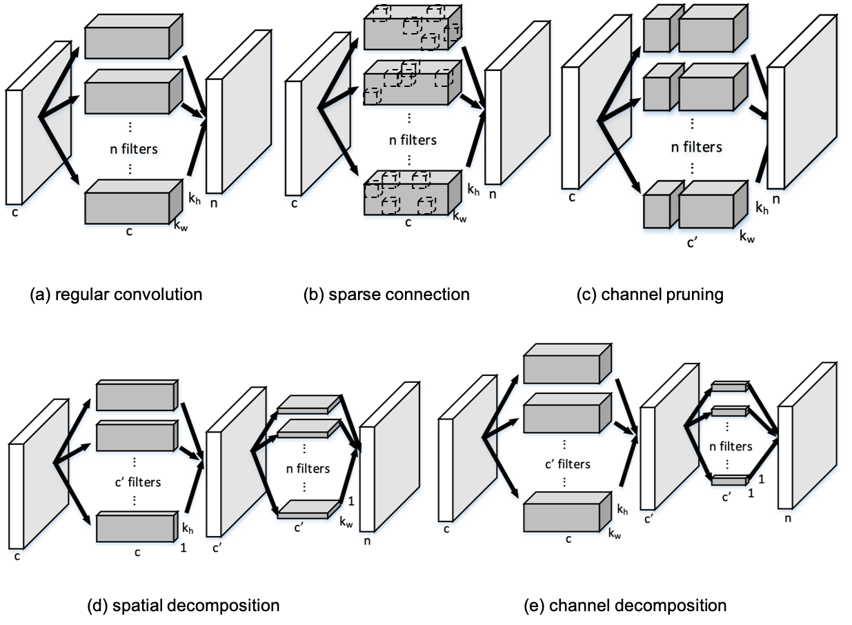
All the recent approaches that try to design compact CNN models mentioned above share a common component: depth-wise separable convolution, initially introduced by [56]. As is pointed out in MobileNets [29], $3\times 3$ depth-wise separable convolutions use between 8 to 9 times less computation than standard convolutions, with the same number of input and output channels. However, inevitably the accuracy is also sacrificed. Although many efforts have been put on searching optimal hyper-parameters for the compact models [77, 60], it remains a question whether we could improve the performance of depth-wise separable convolution itself.

Motivated by this, in this paper, we take the first step towards mitigating the performance degradation of depth-wise separable convolution. Inspired by channel decomposition work [73] which decomposes a standard CNN to a narrower CNN without much degradation (shown in Figure 1 (e)), we propose to decompose an ”unseparated” convolution into a depth-wise separable convolution, while minimizing the performance degradation. Specifically, we first replace all depth-wise separable convolutions in a compact convolutional neural network (e.g., ShuffleNet V2 [47]) with standard convolutions. Then the standard convolutional neural network is trained from scratch on ImageNet. Finally, we decompose the standard convolutions into depth-wise separable convolution to obtain a new compact CNN which is of the same architecture however performs better.

To show the generality of our approach, we conduct rich experiments on ShuffleNet V2 and Xception with the large-scale ImageNet dataset. Using random data, our approach is comparable to channel decomposition [73]. For single layer $9\times$ acceleration, our approach consistently performs better than channel decomposition [73] for different convolutional layers. For decomposition of the ShuffleNet V2 [47] whole model, our approach achieves $\sim$ 2% better Top-1 accuracy than the original ShuffleNet V2.

We summarize our contributions as follow:

1. We propose a novel decomposition approach, namely Depth-wise Decomposition, for expanding regular convolution into depth-wise separable convolution.

2. We take the first step towards improving depth-wise separable convolution performance itself, to the best of our knowledge.

3. Our proposed method improves the Top-1 accuracy of the original model by around 2%.

2 Related Work

Since LeCun et al. introduced optimal brain damage [41, 21], there has been a significant amount of works on accelerating CNNs [6]. Many of them fall into several categories: designing efficient architectures [29, 47], optimized implementation [5], quantization [54], and structured simplification [31].

2.1 Designing Efficient Architecture

Depth-wise separable convolution is widely used in efficient networks like MobileNets [29], ShuffleNets [72] and MnasNets [60]. [15] proved that a regular convolution could be approximated by a combination of several depth-wise separable convolutions. ShiftNets [66] proposed to use shift operation as an alternative to 3-by-3 convolution. AddressNets [25] proposed three shift-based primitives for further improving performance on GPUs (Graphics Processing Units).

2.2 Sparse Connection

Shown in Figure 1 (b), connection pruning eliminates connections between neurons [19, 45, 39, 17, 16]. XNOR-Net [54] binarized the connections. [70] prunes connections based on weights magnitude. Deep compression [18] could accelerate fully connected layers up to $50\times$. However, in practice, the actual speed-up may be strongly related to implementation. The standard library like CUDNN [7] does not support sparse convolution very well. On the contrary, large matrices multiplication is highly optimized.

2.3 Channel Pruning

Shown in Figure 1 (c), channel pruning aims at removing inter-channel redundancies of feature maps. There were several training-based approaches: [2, 65, 75] regularize networks to improve accuracy. Channel-wise SSL [65] reaches high compression ratio for the first few convolutional layers of LeNet [40] and AlexNet [35]. [75] could work well for fully connected layers. However, training-based approaches are more costly, and their effectiveness on very deep networks on large datasets is rarely exploited.

Inference-time channel pruning is challenging, as reported by previous works [3, 53]. Channel pruning [27] proposed to prune neural networks layer-by-layer using LASSO regression and linear least square reconstruction. Some works [57, 49, 30] focus on model size compression, which mainly operate the fully connected layers. Data-free approaches [42, 4] results for speed-up ratio (e.g., $5\times$) have not been reported, and requires long retraining procedure. [4] select channels via over 100 random trials. However, it needs a long time to evaluate each trial on a deep network, which makes it infeasible to work on very deep models and large datasets. Recently, AMC [23, 24] improves general channel pruning approach by learning the speed-up ratio with reinforcement learning.

2.4 Tensor Decomposition

Tensor factorization methods [31, 38, 14, 32] aim to approximate the original convolutional layer weights with several pieces of decomposed weights. Shown in Figure 1 (d), spatial decomposition [31] factorized a layer into $3\times 1$ and $1\times 3$ combination, driven by spatial feature map redundancy. Shown in Figure 1 (e), channel decomposition [73] factorized a layer into $3\times 3$ and $1\times 1$ combination, driven by channel-wise feature map redundancy. [69, 11, 13] accelerate fully connected layers with truncated SVD.

A simple hypothesis is that there is no need to decompose neural networks, simply just train them from scratch. In [73], it has been empirically verified that decomposing neural networks can achieve better performance than naively training them from scratch. This motivates us to decompose regular convolution into depth-wise separable convolution, which could potentially improve the performance of current compact neural networks which favor depth-wise separable convolution a lot.

2.5 Implementation based acceleration

Though convolution is a well defined operation, the run-time can largely depend on the implementations. Optimized implementation based methods [50, 61, 37, 5] accelerate convolution, with special convolution algorithms like FFT [61]. Quantization [9, 54] reduces floating point computational complexity, which is usually followed by fine-tuning and Huffman coding [18]. BinaryNet [9, 52] proposed to binarize both connections and weights. Recently, HAQ [64] automated this process, which further compressed deep neural networks. These methods also depend on the hardware and library implementation.

Figure 2: Depth-wise Decomposition for expanding regular convolution into depth-wise separable convolution

3 Approach

In this section, we first introduce our approach for a special case: single channel convolutional layer. Then we generalize our approach to multi-channel convolutional layer case. Finally, we further generalize our approach for the multi-channel convolutional layer and multi-layers neural networks case.

Let $n$ and $c$ be the number of output and input channels. Let $N$ be the number of samples. Let $k_{h}$ and $k_{w}$ be the kernel size. Let $H$ and $W$ be the spatial size of the feature maps. Formally, we consider a regular convolutional layer shown in the left part of Figure 2, where the weights tensor $W$ ($n\times c\times k_{h}\times k_{w}$) is applied to the input feature maps ($N\times c\times H\times W$) which results in the output feature maps ($N\times n\times H\times W$). The weights tensor can be decomposed into depth-wise convolutional weights $D$ and point-wise convolutional weights $P$ with shape $c\times c\times k_{h}\times k_{w}$ and $n\times c\times 1\times 1$ respectively, shown in the right part of Figure 2. In the following formulations, we do not consider the bias term for simplicity.

3.1 Data Processing

As we can observe, the spatial size $H$ and $W$ are usually large. Following channel decomposition [73], in this paper, we only consider sample patches $Y$ of size ($N\times n$) from the output feature maps and the corresponding $X$ of size ($N\times ck_{h}k_{w}$) from the input feature maps. The spatial size of the $Y$ patches is $1\times 1$. We observe that it is enough to randomly sample 10 patches per image and 300 images in total from the training data to perform our decomposition (In this case, $N=300\times 10$). Convolution can be represented as matrix multiplication in our context:

$$Y=XW$$ (1)

W is the weights matrix ($ck_{h}k_{w}\times n$) reshaped from the original weights tensor.

3.2 A Brief Introduction of Channel Decomposition

Driven by channel-wise feature map redundancy, channel decomposition [73] factorized a convolutional layer ($n\times c\times k_{h}\times k_{w}$) into two convolutional layers: $W_{1}$ ($c^{\prime}\times c\times k_{h}\times k_{w}$) and $W_{2}$ ($n\times c^{\prime}\times 1\times 1$) combination. This is achieved by finding a projection vector $P$ ($n\times c^{\prime}$) such that:

$$\operatorname*{arg\,min}_{V}\lVert Y-YPP^{T}\rVert$$ (2)

This problem can be solved by SVD:

$$U,S,V =SVD(Y)$$ (3)

$P$ is the first $c^{\prime}$ columns of matrix $V$. Then we can obtain $W_{1},W_{2}$ as follow:

$$W_{1} =PW$$ (4)

$$W_{2} =P$$

3.3 Single Channel Case

In this case, we only have a single channel therefore the shape of the layer is $n\times 1\times H\times W$. We aim to decompose the weights tensor ($n\times 1\times k_{h}\times k_{w}$) into a depth-wise tensor $D$ and a point-wise tensors $P$ with shape $1\times 1\times k_{h}\times k_{w}$ and $n\times 1\times 1\times 1$ respectively. Let the output tensor $Y$ be the randomly sampled patches ($N\times n$). Let $V_{0}$ be the projection vector (size $n$). Formally, we try to find $V_{0}$ that minimize:

$$\operatorname*{arg\,min}_{V_{0}}\lVert Y-YV_{0}V_{0}^{T}\rVert$$ (5)

SVD is employed to decompose the output tensor $Y$:

$$U,S,V =SVD(Y)$$ (6)

To construct the two depth-wise and point-wise tensors $D$ and $P$, we extract the projection vector $V_{0}$ (size $n$), namely first column of $V$:

$$D =V_{0}W$$ (7)

$$P =V_{0}$$

Then $D$ and $P$ are reshaped to the tensor format.

3.4 Multi-Channel Case

In single channel case, each channel is approximated into one depth-wise convolutional layer and one point-wise convolutional layer. We can simply apply the single channel algorithm multiple time to each channel of a multi-channel convolutional layer, as is also illustrated in Figure 2:

Algorithm 1 Depth-wise Decomposition

$X_{i}$ is the $i$th channel of feature maps (shape: $N\times k_{h}k_{w}$). $W_{i}$ is the weights connected to $i$th channel (shape: $k_{h}k_{w}\times n$).

initialize D to a zero tensor

initialize P to a zero tensor

for $i\leftarrow 1$ to $c$ do

     $Y_{i}=X_{i}W_{i}$

     $U,S,V=SVD(Y_{i})$

     $D_{i}=V_{0}W_{i}$

     $P_{i}=V_{0}$

end for

return $D$, $P$

3.5 Multi-Channel Case with Inter-channel Error Compensation

Approximation in multi-channel, however, can lead to large approximation error. Thus we propose a novel way to decompose multi-channel sequentially taking into account the approximation errors introduced by decomposition of previous channels (Experiments in Section 4.2). Specifically, instead of purely approximating the output tensor $Y_{i}$, we approximate both the output tensor $Y_{i}$ and approximation error introduced by other channels $E$:

$$\operatorname*{arg\,min}_{V_{0}} \lVert Y_{i}+E-Y_{i}U_{0}V_{0}^{T}\rVert$$ (8)

$$E =\sum_{k=0}^{i-1}E_{k}$$

$$E_{i} =\lvert Y_{i}-Y_{i}U_{0}V_{0}^{T}\rvert$$

where $\lvert\cdot\rvert$ is the absolute value function.

This can be solve by Generalized Singular Value Decomposition (GSVD) [59], without the need of stochastic gradient descent (SGD):

$$U,S,V =GSVD(Y_{i}+E,Y_{i})$$ (9)

$$D_{i} =W_{i}U_{0}$$

$$P_{i} =S_{0}V_{0}$$

Similar with Equation 7, $U_{0}$ and $V_{0}$ are the first columns of matrices $U$ and $V$ respectively.

The Depth-wise Decomposition  with inter-channel error compensation algorithm is as follow:

Algorithm 2 Depth-wise Decomposition with compensation

$X_{i}$ is the $i$th channel of feature maps (shape: $N\times k_{h}k_{w}$). $W_{i}$ is the weights connected to $i$th channel (shape: $k_{h}k_{w}\times n$). $E$ is the tensor of accumulated error.

initialize D to a zero tensor

initialize P to a zero tensor

initialize E to a zero tensor

for $i\leftarrow 1$ to $c$ do

     $Y_{i}=X_{i}W_{i}$

     $U,S,V=GSVD(Y_{i}+E,Y_{i})$

     $D_{i}=W_{i}U_{0}$

     $P_{i}=S_{0}V_{0}$

     $E_{i}=Y_{i}-Y_{i}U_{0}V_{0}^{T}$

     $E=E+E_{i}$

end for

return $D$, $P$

3.6 Multi-layer Case

Finally, our approach can be applied to deep convolutional neural networks layer-by-layer (Section LABEL:sec:multi). Similar with Section 3.5, we can still account for the accumulated error introduced by multi-layer approximation. Here, the error $E^{l}$ in layer $l$ includes both approximation error introduced by decomposing other channels and the previous layer $l-1$. We simply need to extract all feature maps patches $Y_{i}^{\prime}$ before doing decomposition, since the feature map responses will change during decomposition. Similar to the previous sub-section, this problem can be solved by GSVD:

$$\operatorname*{arg\,min}_{V_{0}} \lVert Y_{i}^{\prime}+E^{l}-Y_{i}U_{0}V_{0}^{T}\rVert$$ (10)

$$E^{l} =E^{l-1}+\sum_{k=0}^{i-1}E_{k}$$

$$E_{i} =\lvert Y_{i}^{\prime}-Y_{i}U_{0}V_{0}^{T}\rvert$$

$$U,S,V =GSVD(Y_{i}^{\prime}+E^{l},Y_{i})$$

The following algorithm explains the detailed procedure:

Algorithm 3 Multi-layer Decomposition with compensation

$X_{i}$ is the $i$th channel of feature maps (shape: $N\times k_{h}k_{w}$). $X_{i}^{\prime}$ is the ground truth $i$th channel of feature maps before decomposing the network. $W_{i}$ is the weights connected to $i$th channel (shape: $k_{h}k_{w}\times n$). $E$ is the tensor of accumulated error.

initialize D to a zero tensor

initialize P to a zero tensor

if $l==0$ then

     initialize $E^{l}$ to a zero tensor

else

     initialize $E^{l}$ to the error of previous layer $E^{l-1}$

end if

for $i\leftarrow 1$ to $c$ do

     $Y_{i}^{\prime}=X_{i}^{\prime}W_{i}$

     $Y_{i}=X_{i}W_{i}$

     $U,S,V=GSVD(Y_{i}^{\prime}+E,Y_{i})$

     $D_{i}=W_{i}U_{0}$

     $P_{i}=S_{0}V_{0}$

     $E_{i}=Y_{i}^{\prime}-Y_{i}U_{0}V_{0}^{T}$

     $E^{l}=E^{l}+E_{i}$

end for

return $D$, $P$

3.7 Fine-tuning

Following channel decomposition [73], after a deep convolutional neural network is fully decomposed, we can fine-tune the model for ten epochs with a small learning rate $1e^{-4}$ to obtain better accuracy (Section 4.3).

Unless specified, we do not fine-tune the decomposed model in the following experiments.

4 Experiments

We conduct rich experiments on ImageNet [10] 2012 classification dataset. ImageNet is a very large scale image classification dataset which consists of 1000 classes. Our ShuffleNet V2 model [47] is trained on the 1.3 million training images with 8 GeForce GTX TITAN X GPUs and CUDA 10 [51] CUDNN 7.4 [7]. We also trained a folded ShuffleNet V2 model [47]. In the folded ShuffleNet V2 model [47] we replace every pair of a depthwise convolutional layer and pointwise convolutional layer with a regular convolutional layer. Our model is evaluated on the 50,000 validation images. We evaluate the performance of our approach with top-1 error rate and relative error on ImageNet dataset.

Our neural networks implementation is based on TensorFlow [1]. Our implementation of the previous approach: channel decomposition [73] is based on pure Python.

single layer $9\times$ acceleration with random data
	relative error
Channel Decomposition [73]	$0.887\pm 1.34e^{-6}$
Depth-wise Decomposition (ours)	$0.914\pm 3.21e^{-7}$
Depth-wise Decomposition (ours)	$0.906\pm 2.78e^{-7}$
with compensation

Table 1: Sanity check. Using random data, our approach performs as good as channel decomposition [73]. Standard deviations and relative errors are obtained after 10 runs

4.1 Sanity Check

To check the correctness of our implementation, we created a random weights matrix of size $64\times 128$ and the corresponding random input feature of size $3000\times 64$. The resulting output response is, therefore, a $3000\times 128$ matrix. Our baseline is channel decomposition [73]. Our Depth-wise Decomposition decomposes a convolutional layer into a depth-wise convolution followed by a point-wise convolution, which accelerates the convolutional layer by around $9\times$. For a fair comparison, we use channel decomposition under $9\times$ acceleration.

To measure the correctness of our approach, we measure the relative error of the resulting output responses between those of decomposing algorithms(including baseline [73], Depth-wise Decomposition  and Depth-wise Decomposition  with inter-channel compensation) and the ground-truth output response.

As is shown in Table 1, our Depth-wise Decomposition is comparable to channel decomposition [73].

We further tested the reconstruction error of Depth-wise Decomposition with inter-channel error compensation. As expected, the relative error of this method is smaller than that of our basic approach.

Figure 3: Relative error for decomposing a single conv layer in ShuffleNet V2

Figure 4: Top-1 testing error for decomposing a single convolutional layer in ShuffleNet V2 [47]

Whole Model Decomposition with ImageNet
	top-$1$ error
ShuffleNet V2 [47]	39.7%
Channel Decomposition	40.0%
with fine-tuning [73] (our impl.)
Folded ShuffleNet V2 [47]	36.6%
Depth-wise Decomposition	43.9%
with compensation (ours)
Fine Tuned Depth-wise Decomposition	37.9%
with compensation (ours)

Table 2: Comparisons on compressing ShuffleNet V2 0.5x

4.2 Single Layer Decomposition

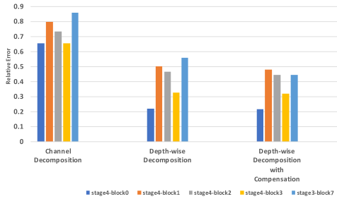
Firstly, we want to evaluate the reconstruction error of Depth-wise Decomposition for a single layer. We conduct experiments on decomposing five different convolutional layers of ShuffleNet V2 [47]. We decompose each 3-by-3 convolutional layer with the baseline method [73], Depth-wise Decomposition and Depth-wise Decomposition with error compensation. Figure 3 shows the relative error of reconstructing each of the five convolutional layers. As shown in the figure, Depth-wise Decomposition results in lower reconstruction error for all five layers. Furthermore, the Depth-wise Decomposition with inter-channel compensation results in even smaller reconstruction error. This proves that both Depth-wise Decomposition and Depth-wise Decomposition with inter-channel error compensation are better at preserving the accuracy of the network while achieving the same level of effectiveness in terms of accelerating the network.

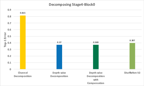
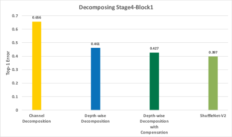
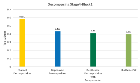
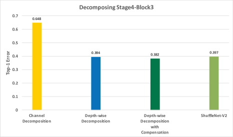
Secondly, we want to measure the effectiveness of Depth-wise Decomposition. Thus we measure how much the top-1 error of the resulting network has increased when decomposing a single convolutional layer in ShuffleNet V2 [47]. We demonstrate the effectiveness of Depth-wise Decomposition by showing the top-1 error of the networks resulting from decomposing each of the four convolutional layers in stage 4 of ShuffleNet V2 [47] along with the top-1 error achieved by the original ShuffleNet V2 [47] model. As shown in Figure  4, the baseline method [73], when accelerating one convolutional layer by around $9\times$, largely increases the top-1 error of the resulting network. In contrast, Depth-wise Decomposition, along with Depth-wise Decomposition with error compensation do not have such a significant impact on the top-1 error of the resulting network.

4.3 Whole Model Decomposition

Lastly we want to measure the effect of decomposing the whole model. First we train a ”folded” ShuffleNet V2 [47]. In this model we replace depth-wise separable convolutional layers with regular convolutional layers. For example, a depth-wise convolution layer with shape $C\times C\times k_{h}\times k_{w}$ and a point-wise convolution with shape $N\times C\times 1\times 1$ will be replaced by a regular convolutional layer with shape $N\times C\times k_{h}\times k_{w}$. We train this model with the exact same settings as the original ShuffleNets V2 paper. Our implementation is based on TensorPack [67]. Shown in Table 2, the Top-1 accuracy of ”folded” ShuffleNet V2 is 3.1% higher than the original ShuffleNet V2, which serves as the upper bound of our proposed algorithm.

Then we decompose each convolutional layers in the folded ShuffleNet V2 [47] using our multi-layer channel decomposition method with inter-channel error compensation (Section 3.6). This decomposed model has the exact same architecture as the original ShuffleNet V2. Then the decomposed model is further fine-tuned on ImageNet training dataset for 10 epochs (Section 3.7).

As a baseline, we perform channel decomposition [73] under $9\times$ acceleration ratio on ShuffleNet V2 and fine-tune for the same number of epochs as our model. However, channel decomposition does not work well for high acceleration ratio in our case. Shown in Table 2, it even performs worse than the original ShuffleNet V2.

As is shown in Table 2, our Depth-wise Decomposition with inter-channel error compensation has $\sim$ 2% lower top-1 error than the original ShuffleNet V2 [47]. It proves that our method is able to achieve a better level of accuracy under the same computational complexity compare to ShuffleNet V2 [47].

top-$1$ error	baseline	ours
ShuffleNet V2 0.5$\times$ [47]	39.7%	37.9%
ShuffleNet V2 1.0$\times$ [47]	30.6%	28.0%
ShuffleNet V2 2.0$\times$ [47]	25.1%	23.4%
Xception [8]	21.0%	20.1%

Table 3: Top-1 error for compressing ShuffleNet V2 family and Xception

To test the generalizability of our approach, we further test on other ShuffleNet V2 architectures and Xception. Shown in Table 3, The results are consistent with ShuffleNet v2 $0.5\times$ in Table 2. For ShuffleNet v2 $1\times$, our approach improves the Top-1 accuracy by 1.6%. For ShuffleNet v2 $2\times$, the Top-1 accuracy improvement is 1.7%. For Xception, the model performs 1.6% better.

5 Conclusion

In conclusion, very deep convolutional neural networks (CNNs) are widely used among many computer vision tasks. However, most state-of-the-art CNNs are large, which results in high inference latency. Recent depth-wise separable convolution has been proposed for image recognition tasks on the computationally limited platforms. Though it is much faster than regular convolution, accuracy is sacrificed. In this paper, we propose a novel decomposition approach based on SVD, namely depth-wise decomposition, for expanding regular convolution into depth-wise separable convolution while maintaining high accuracy. Thorough experiments with the latest ShuffleNet V2 model [47] on ImageNet [10] have verified the effectiveness of our approach.

References

- [1] Martín Abadi, Paul Barham, Jianmin Chen, Zhifeng Chen, Andy Davis, Jeffrey Dean, Matthieu Devin, Sanjay Ghemawat, Geoffrey Irving, Michael Isard, et al. Tensorflow: a system for large-scale machine learning. In OSDI, volume 16, pages 265–283, 2016.
- [2] Jose M Alvarez and Mathieu Salzmann. Learning the number of neurons in deep networks. In Advances in Neural Information Processing Systems, pages 2262–2270, 2016.
- [3] Sajid Anwar, Kyuyeon Hwang, and Wonyong Sung. Structured pruning of deep convolutional neural networks. arXiv preprint arXiv:1512.08571, 2015.
- [4] Sajid Anwar and Wonyong Sung. Compact deep convolutional neural networks with coarse pruning. arXiv preprint arXiv:1610.09639, 2016.
- [5] Hessam Bagherinezhad, Mohammad Rastegari, and Ali Farhadi. Lcnn: Lookup-based convolutional neural network. arXiv preprint arXiv:1611.06473, 2016.
- [6] Yu Cheng, Duo Wang, Pan Zhou, and Tao Zhang. A survey of model compression and acceleration for deep neural networks. arXiv preprint arXiv:1710.09282, 2017.
- [7] Sharan Chetlur, Cliff Woolley, Philippe Vandermersch, Jonathan Cohen, John Tran, Bryan Catanzaro, and Evan Shelhamer. cudnn: Efficient primitives for deep learning. arXiv preprint arXiv:1410.0759, 2014.
- [8] François Chollet. Xception: Deep learning with depthwise separable convolutions. arXiv preprint, pages 1610–02357, 2017.
- [9] Matthieu Courbariaux and Yoshua Bengio. Binarynet: Training deep neural networks with weights and activations constrained to+ 1 or-1. arXiv preprint arXiv:1602.02830, 2016.
- [10] Jia Deng, Wei Dong, Richard Socher, Li-Jia Li, Kai Li, and Li Fei-Fei. Imagenet: A large-scale hierarchical image database. In Computer Vision and Pattern Recognition, 2009. CVPR 2009. IEEE Conference on, pages 248–255. IEEE, 2009.
- [11] Emily L Denton, Wojciech Zaremba, Joan Bruna, Yann LeCun, and Rob Fergus. Exploiting linear structure within convolutional networks for efficient evaluation. In Advances in Neural Information Processing Systems, pages 1269–1277, 2014.
- [12] Nemanja Djuric, Vladan Radosavljevic, Henggang Cui, Thi Nguyen, Fang-Chieh Chou, Tsung-Han Lin, and Jeff Schneider. Motion prediction of traffic actors for autonomous driving using deep convolutional networks. arXiv preprint arXiv:1808.05819, 2018.
- [13] Ross Girshick. Fast r-cnn. In Proceedings of the IEEE International Conference on Computer Vision, pages 1440–1448, 2015.
- [14] Yunchao Gong, Liu Liu, Ming Yang, and Lubomir Bourdev. Compressing deep convolutional networks using vector quantization. arXiv preprint arXiv:1412.6115, 2014.
- [15] Jianbo Guo, Yuxi Li, Weiyao Lin, Yurong Chen, and Jianguo Li. Network decoupling: From regular to depthwise separable convolutions. arXiv preprint arXiv:1808.05517, 2018.
- [16] Yiwen Guo, Anbang Yao, and Yurong Chen. Dynamic network surgery for efficient dnns. In Advances In Neural Information Processing Systems, pages 1379–1387, 2016.
- [17] Song Han, Xingyu Liu, Huizi Mao, Jing Pu, Ardavan Pedram, Mark A Horowitz, and William J Dally. Eie: efficient inference engine on compressed deep neural network. In Proceedings of the 43rd International Symposium on Computer Architecture, pages 243–254. IEEE Press, 2016.
- [18] Song Han, Huizi Mao, and William J Dally. Deep compression: Compressing deep neural network with pruning, trained quantization and huffman coding. CoRR, abs/1510.00149, 2, 2015.
- [19] Song Han, Jeff Pool, John Tran, and William Dally. Learning both weights and connections for efficient neural network. In Advances in Neural Information Processing Systems, pages 1135–1143, 2015.
- [20] Bharath Hariharan, Pablo Arbeláez, Ross Girshick, and Jitendra Malik. Hypercolumns for object segmentation and fine-grained localization. In Proceedings of the IEEE conference on computer vision and pattern recognition, pages 447–456, 2015.
- [21] Babak Hassibi and David G Stork. Second order derivatives for network pruning: Optimal brain surgeon. Morgan Kaufmann, 1993.
- [22] Kaiming He, Xiangyu Zhang, Shaoqing Ren, and Jian Sun. Deep residual learning for image recognition. In Proceedings of the IEEE Conference on Computer Vision and Pattern Recognition, pages 770–778, 2016.
- [23] Yihui He and Song Han. Adc: Automated deep compression and acceleration with reinforcement learning. arXiv preprint arXiv:1802.03494, 2018.
- [24] Yihui He, Ji Lin, Zhijian Liu, Hanrui Wang, Li-Jia Li, and Song Han. Amc: Automl for model compression and acceleration on mobile devices. In Proceedings of the European Conference on Computer Vision (ECCV), pages 784–800, 2018.
- [25] Yihui He, Xianggen Liu, Huasong Zhong, and Yuchun Ma. Addressnet: Shift-based primitives for efficient convolutional neural networks. In 2019 IEEE Winter Conference on Applications of Computer Vision (WACV), pages 1213–1222. IEEE, 2019.
- [26] Yihui He, Xiangyu Zhang, Marios Savvides, and Kris Kitani. Softer-nms: Rethinking bounding box regression for accurate object detection. arXiv preprint arXiv:1809.08545, 2018.
- [27] Yihui He, Xiangyu Zhang, and Jian Sun. Channel pruning for accelerating very deep neural networks. In International Conference on Computer Vision (ICCV), volume 2, 2017.
- [28] Yihui He, Chenchen Zhu, Jianren Wang, Marios Savvides, and Xiangyu Zhang. Bounding box regression with uncertainty for accurate object detection. In 2019 IEEE Conference on Computer Vision and Pattern Recognition (CVPR). IEEE, 2019.
- [29] Andrew G Howard, Menglong Zhu, Bo Chen, Dmitry Kalenichenko, Weijun Wang, Tobias Weyand, Marco Andreetto, and Hartwig Adam. Mobilenets: Efficient convolutional neural networks for mobile vision applications. arXiv preprint arXiv:1704.04861, 2017.
- [30] Hengyuan Hu, Rui Peng, Yu-Wing Tai, and Chi-Keung Tang. Network trimming: A data-driven neuron pruning approach towards efficient deep architectures. arXiv preprint arXiv:1607.03250, 2016.
- [31] Max Jaderberg, Andrea Vedaldi, and Andrew Zisserman. Speeding up convolutional neural networks with low rank expansions. arXiv preprint arXiv:1405.3866, 2014.
- [32] Yong-Deok Kim, Eunhyeok Park, Sungjoo Yoo, Taelim Choi, Lu Yang, and Dongjun Shin. Compression of deep convolutional neural networks for fast and low power mobile applications. arXiv preprint arXiv:1511.06530, 2015.
- [33] Animesh Koratana, Daniel Kang, Peter Bailis, and Matei Zaharia. Lit: Block-wise intermediate representation training for model compression. arXiv preprint arXiv:1810.01937, 2018.
- [34] Ranjay Krishna, Yuke Zhu, Oliver Groth, Justin Johnson, Kenji Hata, Joshua Kravitz, Stephanie Chen, Yannis Kalantidis, Li-Jia Li, David A Shamma, et al. Visual genome: Connecting language and vision using crowdsourced dense image annotations. International Journal of Computer Vision, 123(1):32–73, 2017.
- [35] Alex Krizhevsky, Ilya Sutskever, and Geoffrey E Hinton. Imagenet classification with deep convolutional neural networks. In Advances in neural information processing systems, pages 1097–1105, 2012.
- [36] Athindran Ramesh Kumar, Balaraman Ravindran, and Anand Raghunathan. Pack and detect: Fast object detection in videos using region-of-interest packing. In Proceedings of the ACM India Joint International Conference on Data Science and Management of Data, pages 150–156. ACM, 2019.
- [37] Andrew Lavin. Fast algorithms for convolutional neural networks. arXiv preprint arXiv:1509.09308, 2015.
- [38] Vadim Lebedev, Yaroslav Ganin, Maksim Rakhuba, Ivan Oseledets, and Victor Lempitsky. Speeding-up convolutional neural networks using fine-tuned cp-decomposition. arXiv preprint arXiv:1412.6553, 2014.
- [39] Vadim Lebedev and Victor Lempitsky. Fast convnets using group-wise brain damage. arXiv preprint arXiv:1506.02515, 2015.
- [40] Yann LeCun, Léon Bottou, Yoshua Bengio, and Patrick Haffner. Gradient-based learning applied to document recognition. Proceedings of the IEEE, 86(11):2278–2324, 1998.
- [41] Yann LeCun, John S Denker, Sara A Solla, Richard E Howard, and Lawrence D Jackel. Optimal brain damage. In NIPs, volume 2, pages 598–605, 1989.
- [42] Hao Li, Asim Kadav, Igor Durdanovic, Hanan Samet, and Hans Peter Graf. Pruning filters for efficient convnets. arXiv preprint arXiv:1608.08710, 2016.
- [43] Yudong Liang, Ze Yang, Kai Zhang, Yihui He, Jinjun Wang, and Nanning Zheng. Single image super-resolution via a lightweight residual convolutional neural network. arXiv preprint arXiv:1703.08173, 2017.
- [44] Tsung-Yi Lin, Michael Maire, Serge Belongie, James Hays, Pietro Perona, Deva Ramanan, Piotr Dollár, and C Lawrence Zitnick. Microsoft coco: Common objects in context. In European conference on computer vision, pages 740–755. Springer, Cham, 2014.
- [45] Baoyuan Liu, Min Wang, Hassan Foroosh, Marshall Tappen, and Marianna Pensky. Sparse convolutional neural networks. In Proceedings of the IEEE Conference on Computer Vision and Pattern Recognition, pages 806–814, 2015.
- [46] Jonathan Long, Evan Shelhamer, and Trevor Darrell. Fully convolutional networks for semantic segmentation. In Proceedings of the IEEE conference on computer vision and pattern recognition, pages 3431–3440, 2015.
- [47] Ningning Ma, Xiangyu Zhang, Hai-Tao Zheng, and Jian Sun. Shufflenet v2: Practical guidelines for efficient cnn architecture design. In The European Conference on Computer Vision (ECCV), September 2018.
- [48] Xiaobo Ma, Yihui He, Xiapu Luo, Jianfeng Li, Mengchen Zhao, Bo An, and Xiaohong Guan. Camera placement based on vehicle traffic for better city security surveillance. IEEE Intelligent Systems, 33(4):49–61, 2018.
- [49] Zelda Mariet and Suvrit Sra. Diversity networks. arXiv preprint arXiv:1511.05077, 2015.
- [50] Michael Mathieu, Mikael Henaff, and Yann LeCun. Fast training of convolutional networks through ffts. arXiv preprint arXiv:1312.5851, 2013.
- [51] John Nickolls, Ian Buck, Michael Garland, and Kevin Skadron. Scalable parallel programming with cuda. In ACM SIGGRAPH 2008 classes, page 16. ACM, 2008.
- [52] Hai Phan, Dang Huynh, Yihui He, Marios Savvides, and Zhiqiang Shen. Mobinet: A mobile binary network for image classification. In 2020 IEEE Winter Conference on Applications of Computer Vision (WACV). IEEE, 2020.
- [53] Adam Polyak and Lior Wolf. Channel-level acceleration of deep face representations. IEEE Access, 3:2163–2175, 2015.
- [54] Mohammad Rastegari, Vicente Ordonez, Joseph Redmon, and Ali Farhadi. Xnor-net: Imagenet classification using binary convolutional neural networks. In European Conference on Computer Vision, pages 525–542. Springer, 2016.
- [55] Shaoqing Ren, Kaiming He, Ross Girshick, and Jian Sun. Faster r-cnn: Towards real-time object detection with region proposal networks. In Advances in neural information processing systems, pages 91–99, 2015.
- [56] Laurent Sifre and Stéphane Mallat. Rigid-motion scattering for image classification. PhD thesis, Citeseer, 2014.
- [57] Suraj Srinivas and R Venkatesh Babu. Data-free parameter pruning for deep neural networks. arXiv preprint arXiv:1507.06149, 2015.
- [58] Christian Szegedy, Wei Liu, Yangqing Jia, Pierre Sermanet, Scott Reed, Dragomir Anguelov, Dumitru Erhan, Vincent Vanhoucke, and Andrew Rabinovich. Going deeper with convolutions. In Proceedings of the IEEE conference on computer vision and pattern recognition, pages 1–9, 2015.
- [59] Yoshio Takane and Heungsun Hwang. Regularized linear and kernel redundancy analysis. Computational Statistics & Data Analysis, 52(1):394–405, 2007.
- [60] Mingxing Tan, Bo Chen, Ruoming Pang, Vijay Vasudevan, and Quoc V Le. Mnasnet: Platform-aware neural architecture search for mobile. arXiv preprint arXiv:1807.11626, 2018.
- [61] Nicolas Vasilache, Jeff Johnson, Michael Mathieu, Soumith Chintala, Serkan Piantino, and Yann LeCun. Fast convolutional nets with fbfft: A gpu performance evaluation. arXiv preprint arXiv:1412.7580, 2014.
- [62] Jianren Wang, Yihui He, Xiaobo Wang, Xinjia Yu, and Xia Chen. Prediction-tracking-segmentation. arXiv preprint arXiv:1904.03280, 2019.
- [63] Jianren Wang, Junkai Xu, and Peter B Shull. Vertical jump height estimation algorithm based on takeoff and landing identification via foot-worn inertial sensing. Journal of biomechanical engineering, 140(3):034502, 2018.
- [64] Kuan Wang, Zhijian Liu, Yujun Lin, Ji Lin, and Song Han. Haq: Hardware-aware automated quantization. arXiv preprint arXiv:1811.08886, 2018.
- [65] Wei Wen, Chunpeng Wu, Yandan Wang, Yiran Chen, and Hai Li. Learning structured sparsity in deep neural networks. In Advances In Neural Information Processing Systems, pages 2074–2082, 2016.
- [66] Bichen Wu, Alvin Wan, Xiangyu Yue, Peter Jin, Sicheng Zhao, Noah Golmant, Amir Gholaminejad, Joseph Gonzalez, and Kurt Keutzer. Shift: A zero flop, zero parameter alternative to spatial convolutions. arXiv preprint arXiv:1711.08141, 2017.
- [67] Yuxin Wu et al. Tensorpack. github.com/tensorpack/, 2016.
- [68] Haisheng Xia, Junkai Xu, Jianren Wang, Michael A Hunt, and Peter B Shull. Validation of a smart shoe for estimating foot progression angle during walking gait. Journal of biomechanics, 61:193–198, 2017.
- [69] Jian Xue, Jinyu Li, and Yifan Gong. Restructuring of deep neural network acoustic models with singular value decomposition. In INTERSPEECH, pages 2365–2369, 2013.
- [70] Tien-Ju Yang, Yu-Hsin Chen, and Vivienne Sze. Designing energy-efficient convolutional neural networks using energy-aware pruning. arXiv preprint arXiv:1611.05128, 2016.
- [71] Matthew D Zeiler and Rob Fergus. Visualizing and understanding convolutional networks. In European conference on computer vision, pages 818–833. Springer, 2014.
- [72] X Zhang, X Zhou, M Lin, and J Sun. Shufflenet: An extremely efficient convolutional neural network for mobile devices. arxiv 2017. arXiv preprint arXiv:1707.01083.
- [73] Xiangyu Zhang, Jianhua Zou, Kaiming He, and Jian Sun. Accelerating very deep convolutional networks for classification and detection. IEEE transactions on pattern analysis and machine intelligence, 38(10):1943–1955, 2016.
- [74] Bolei Zhou, Hang Zhao, Xavier Puig, Sanja Fidler, Adela Barriuso, and Antonio Torralba. Scene parsing through ade20k dataset. In Proceedings of the IEEE Conference on Computer Vision and Pattern Recognition, 2017.
- [75] Hao Zhou, Jose M Alvarez, and Fatih Porikli. Less is more: Towards compact cnns. In European Conference on Computer Vision, pages 662–677. Springer International Publishing, 2016.
- [76] Chenchen Zhu, Yihui He, and Marios Savvides. Feature selective anchor-free module for single-shot object detection. arXiv preprint arXiv:1903.00621, 2019.
- [77] Barret Zoph, Vijay Vasudevan, Jonathon Shlens, and Quoc V Le. Learning transferable architectures for scalable image recognition. arXiv preprint arXiv:1707.07012, 2(6), 2017.