Low-Rank plus Sparse Decomposition of Covariance Matrices
using Neural Network Parametrization

Low-Rank plus Sparse Decomposition
of Covariance Matrices
using Neural Network Parametrization

Abstract

This paper revisits the problem of decomposing a positive semidefinite matrix as a sum of a matrix with a given rank plus a sparse matrix. An immediate application can be found in portfolio optimization, when the matrix to be decomposed is the covariance between the different assets in the portfolio. Our approach consists in representing the low-rank part of the solution as the product $MM^{T}$, where $M$ is a rectangular matrix of appropriate size, parametrized by the coefficients of a deep neural network. We then use a gradient descent algorithm to minimize an appropriate loss function over the parameters of the network. We deduce its convergence rate to a local optimum from the Lipschitz smoothness of our loss function. We show that the rate of convergence grows polynomially in the dimensions of the input, output, and the size of each of the hidden layers.

I Introduction

We present a new approach to decompose a possibly large covariance matrix $\Sigma$ into the sum of a positive semidefinite low-rank matrix $L$ plus a sparse matrix $S$. Our approach consists in fixing an (upper bound for the) rank $k$ of $L$ by defining $L:=MM^{T}$ for a suitable $M\in\mathbb{R}^{n\times k}$, where one parametrizes $M$ using a deep neural network, whose coefficients are minimized using a gradient descent method.

Albeit our method can be used in any context where such a problem occurs, our primary application of interest is rooted in Finance. When studying the correlation matrix between the returns of financial assets, it is important for the design of a well-diversified portfolio to identify groups of heavily correlated assets, or more generally, to identify a few ad-hoc features, or economic factors, that describe some dependencies between these assets. To this effect, the most natural tool is to determine the few first dominant eigenspaces of the correlation matrix and to interpret them as the main features driving the behavior of the portfolio. This procedure, generally termed Principal Component Analysis (PCA), is widely used. However, PCA does not ensure any sparsity between the original matrix $\Sigma$ and its approximation $A$. As it turns out, many coefficients of $\Sigma-A$ can be relatively large with respect to the others; these indicate pairs of assets that present an ignored large correlation between themselves, beyond the dominant features revealed by PCA. Following [24], to reveal this extra structure present in $\Sigma$, we decompose it into the sum of a low-rank matrix $L$, which describes the dominant economic factors of a portfolio, plus a sparse matrix $S$, to identify hidden large correlations between assets pairs. The number of those economic factors is set according to the investor’s views on the market, and coincides with the rank of $L$. The sparse part $S$ can be seen as a list of economic abnormalities, which can be exploited by the investor.

Beyond covariance matrices, this decomposition is a procedure abundantly used in image and video processing for compression and interpretative purposes [3], but also in latent variable model selection [6], in latent semantic indexing [16], in graphical model selection [2], in graphs [23], and in gene expression [14], among others. A rich collection of algorithms exist to compute such decomposition, see [7, 9, 13, 25, 26] to cite but a few, most of which are reviewed in [4] and implemented in the Matlab LRS library [5]. However, our method can only address the decomposition of a symmetric positive semidefinite matrix, as it uses explicitly and takes full advantage of this very particular structure.

The Principal Component Pursuit (PCP) reformulation of this problem has been proposed and studied by [6, 7, 13] as a robust alternative to PCA, and generated a number of efficient algorithms. For a given $\delta>0$, the PCP problem is formulated as

$$\min_{L,S}||L||_{*}+\delta||S||_{1}\quad\operatorname{s.\!t.\,}\Sigma=L+S\,.$$ (1)

where $\Sigma\in\mathbb{R}^{n\times n}$ is the observed matrix, $||L||_{*}$ is the nuclear norm of matrix $L$ (i.e. the sum of all singular values of $L$) and $||S||_{1}$ is the $l^{1}$-norm of matrix $S$. To solve (1), an approach consists in constructing its Augmented Lagrange Multiplier (ALM) [10]. By incorporating the constraints of (1) into the objective multiplied by their Lagrange multiplier $Y\in\mathbb{R}^{n\times n}$, the ALM is

$$\min_{L,S,Y}||L||_{*}+\delta||S||_{1}+\langle Y,\Sigma-L-S\rangle+\frac{\mu}{2}||\Sigma-L-S||^{2}_{F}\,,$$ (2)

which coincides with the original problem when $\mu\to\infty$. We denote by $\mathcal{L}_{\mu}(L,S,Y)$ the above objective function. In [13], it is solved with an alternating direction method:

$$L_{t+1} =\arg\min_{L}\mathcal{L}_{\mu_{t}}(L,S_{t},Y_{t})$$ (3)

$$S_{t+1} =\arg\min_{S}\mathcal{L}_{\mu_{t}}(L_{t+1},S,Y_{t})$$ (4)

$$Y_{t+1} =Y_{t}+\mu_{t}(\Sigma-L_{t+1}-S_{t+1})$$

$$\mu_{t+1} =\rho\mu_{t}.$$

for some $\rho>1$. The resulting method is called Inexact ALM (IALM); in the Exact ALM, $\mathcal{L}_{\mu}(L,S,Y_{t})$ is minimized on $L$ and $S$ simultaneously, a considerably more difficult task. The problem (4) can be solved explicitly at modest cost. In contrast, (3) requires an expensive Singular Value Decomposition (SVD). In [12], the authors replace the nuclear norm in (2) by the non-convex function $||L||_{\gamma}:=\sum_{i}(1+\gamma)\sigma_{i}(L)/(\gamma+\sigma_{i}(L))$ that interpolates between $\operatorname{rank}(L)$ and $||X||_{*}$ as $\gamma$ goes from $0$ to $1$, in order to depart from the convex PCP approximation of the original problem. Then they apply the same alternating direction method to the resulting function. This method is referred to as Non-Convex RCPA or NC-RCPA. In [21], the authors rather solve a variant of (1) by incorporating the constraint into the objective, removing the costly nuclear norm term, and imposing a rank constraint on $L$:

$$\min_{L,S}\delta||S||_{1}+\frac{1}{2}||\Sigma-L-S||^{2}_{F}\quad\operatorname{s.\!t.\,}\operatorname{rank}(L)=k.$$ (5)

We denote by $\widehat{\mathcal{L}}(L,S)$ the above objective function. Using also an alternating direction strategy, the authors have devised the Fast PCP (FPCP) method as

$$L_{t+1} =\arg\min_{L}\widehat{\mathcal{L}}(L,S_{t})\ \ \operatorname{s.\!t.\,}\operatorname{rank}(L)=k$$ (6)

$$S_{t+1} =\arg\min_{S}\widehat{\mathcal{L}}(L_{t+1},S).$$ (7)

The problem (7) is easy to solve as for (4). In contrast to (3), the sub-problem (6) can be solved by applying a faster partial SVD to $\Sigma-S_{t}$, with the only necessity of computing the $k$ first singular values and their associated eigenvectors. These authors have further improved their algorithm in [22] with an accelerated variant of the partial SVD algorithm. Their methods are considered as state-of-the-art in the field [4] and their solution is of comparable quality to the one of (1). An alternative approach, designated here as (RPCA-GD) to solve (5) was proposed in [27], where, as in our setting, the rank constraint is enforced by setting $L:=MM^{T}$ for $M\in\mathbb{R}^{n\times k}$. Then a projected gradient method is used to solve (6) in $M$. In order to guarantee that $S$ has a prescribed sparsity, they use an ad-hoc projector on an appropriate space of sparse matrices.

The solution to the PCP problem (1) depends on the hyperparameter $\delta$, from which we cannot infer the value of the rank $k$ of the resulting optimal $L$ with more accuracy than in the classical results of Candès et al. in Theorem 1.1 of [6]. In view of the particular financial application we have in mind, we would prefer a method for which we can chose the desired $k$ in advance. In both the IALM and the Non-Convex RPCA methods, neither the rank of $L$ nor its expressivity — that is, the portion of the spectrum of $\Sigma$ covered by the low-rank matrix — can be chosen in advance. In RPCA-GD, the rank is chosen in advance, but the sparsity of $S$ is set in advance by inspection of the given matrix $\Sigma$, a limitation that we would particularly like to avoid in our application. From this point of view, FPCP seems the most appropriate method. In our approach, we must first select a rank for $L$, based e.g. on a prior spectral decomposition of $\Sigma$ or based on exogenous considerations. We then apply a gradient descent method with a well-chosen loss function, using Tensorflow [1] or Pytorch [20].

In Section II, we introduce the construction of our low-rank matrix $L=MM^{T}$, where $M$, in contrast with the RPCA-GD method, is parametrized by the coefficients of a multi-layered neural network. A potential advantage of this parametrization has been pointed in [15], albeit in a different context than ours. We also describe the corresponding loss function that we seek to minimize. Moreover, we analyze the regularity properties of the objective function leading to an estimate of the convergence rate of a standard gradient descent method to a stationary point of the method; see Theorem II.1. We show that the convergence rate of our algorithm grows polynomially in the dimension of each layer. In Section III, we conduct a series of experiments first on artificially generated data, that is matrices $\Sigma$ with a given decomposition $L+S$, to assess the accuracy of our method and to compare it with the algorithms presented in this section. We apply also our algorithm to real data sets: the correlation matrix of the stocks from the S&P500 index and an estimate of the correlation matrix between real estate market indices of 44 countries. We show that our method achieves a higher accuracy than the other algorithms. Moreover, by its construction of $L:=MM^{T}$, we can guarantee the positive semidefiniteness of $L$, although empirical covariance matrices tend to not satisfy this property. We refer to [11] for a detailed discussion of this issue. By contrast, most algorithms do not ensure that $L$ is kept positive semidefinite, which forces them to correct their output at the expense of their accuracy. The proof of Theorem II.1 is provided in Section IV.

II Neural network parametrized optimization and its convergence rate

Let $\mathbb{S}^{n}$ be the set of $n$-by-$n$ real symmetric matrices and $\mathbb{S}^{n}_{+}\subset\mathbb{S}^{n}$ be the cone of positive semidefinite matrices. We are given a matrix $\Sigma=\left[\Sigma_{i,j}\right]_{i,j}\in\mathbb{S}^{n}$ and a number $1\leq k\leq n$. Our task is to decompose $\Sigma$ as the sum of $L=\left[L_{i,j}\right]_{i,j}\in\mathbb{S}^{n}_{+}$ of rank at most equal $k$ and a sparse matrix $S=\left[S_{i,j}\right]_{i,j}\in\mathbb{R}^{n\times n}$ in some optimal way. Observe that the matrix $S$ is also a symmetric matrix. It is well-known that the matrix $L$ can be represented as $L=MM^{T}$, where $M=\left[M_{i,j}\right]_{i,j}\in\mathbb{R}^{n\times k}$; thus $\Sigma=MM^{T}+S$.

For practical purposes, we shall represent every symmetric $n$-by-$n$ matrix by a vector of dimension $r:=n(n+1)/2$; formally, we define the linear operator

$$h:\mathbb{S}^{n} \to \mathbb{R}^{n(n+1)/2},$$ (8)

$$\Sigma \mapsto h(\Sigma):=(\Sigma_{1,1},\dots,\Sigma_{1,n},\Sigma_{2,2},\dots,\Sigma_{2,n},\dots,\Sigma_{n,n})^{T}.$$

The operator $h$ is obviously invertible, and its inverse shall be denoted by $h^{-1}$. Similarly, every vector of dimension $nk$ shall be represented by a $n$-by-$k$ matrix by the linear operator $g:\mathbb{R}^{nk}\to\mathbb{R}^{n\times k}$, which maps $v=(v_{1},\ldots,v_{nk})^{T}$ to $g(v):=W\equiv[w_{i,j}]_{i,j}$ with $w_{i,j}=v_{(i-1)k+j}$, in a kind of row-after-row filling of $W$ by $v$. This operator has clearly an inverse $g^{-1}$.

We construct a neural network with $n(n+1)/2$ inputs and $nk$ outputs; these outputs are meant to represent the coefficients of the matrix $M$ with whom we shall construct the rank $k$ matrix $L$ in the decomposition of the input matrix $\Sigma$. However, we do not use this neural network in its feed-forward mode as a heuristic to compute $M$ from an input $\Sigma$; we merely use the neural network framework as a way to parametrize a tentative solution $M$ to our decomposition problem.

We construct our neural network with $m$ layers of respectively $\ell_{1},\ldots,\ell_{m}$ neurons, each with the same activation function $\sigma:\mathbb{R}\to[-1,1]$. We assume that the first and the second derivative of $\sigma$ are uniformly bounded from above by the constants $\sigma^{\prime}_{\textrm{max}}>0$ and $\sigma^{\prime\prime}_{\textrm{max}}$, respectively. We let $\ell_{0}:=n(n+1)/2$ and $\ell_{m+1}:=nk$. In accordance with the standard architecture of fully connected multi-layered neural networks, for $0\leq u\leq m$ we let $A^{(u)}=\left[A^{(u)}_{i,j}\right]_{i,j}\in\mathbb{R}^{\ell_{u+1}\times\ell_{u}}$ be layer $u$’s weights,
$b^{(u)}=\left[b^{(u)}_{i}\right]_{i}\in\mathbb{R}^{\ell_{u+1}}$ be its bias, and for all $v\in\mathbb{R}^{\ell_{u}}$

$$f_{u}^{A^{(u)},b^{(u)}}(v):=A^{(u)}v+b^{(u)}.$$

For each $1\leq i\leq m$ and each $v\in\mathbb{R}^{\ell_{i}}$, we write $\sigma^{(i)}(v):=\left(\sigma(v_{1}),\ldots,\sigma(v_{\ell_{i}})\right)^{T}$. We denote the parameters $\Theta:=(A^{(0)},b^{(0)},\dots,A^{(m)},b^{(m)})$ and define the $m$-layered neural network by the function $\mathcal{N}^{\Theta}_{m}$ from $\mathbb{R}^{\ell_{0}}$ to $\mathbb{R}^{\ell_{m+1}}$ for which $\mathcal{N}^{\Theta}_{m}(x)$ equals

$$\begin{split}f_{m}^{A^{(m)},b^{(m)}}\!\circ\!\sigma^{(m)}\circ f_{m-1}^{A^{(m-1)},b^{(m-1)}}\!\circ\!\dots\!\circ\!\sigma^{(1)}\!\circ\!f_{0}^{A^{(0)},b^{(0)}}(x).\end{split}$$

We therefore have to specify $\mathbb{L}_{m}:=\sum_{u=0}^{m}\ell_{u}\ell_{u+1}+\ell_{u+1}$ many parameters to describe the neural network $\mathcal{N}^{\Theta}_{m}$ completely.

Now, we are ready to define the cost function to minimize. We write the $1$-norm of some $X\in\mathbb{R}^{n\times n}$ as $||X||_{1}:=\sum_{i,j=1}^{n}|X_{i,j}|$. Our objective function is, for a given $\Sigma\in\mathbb{S}^{n}$, the function

$$\varphi_{\mathrm{obj}}(\Theta):=\left\|g\big{(}\mathcal{N}^{\Theta}_{m}\left(h(\Sigma)\right)\!\big{)}\,g\big{(}\mathcal{N}^{\Theta}_{m}\left(h(\Sigma)\right)\!\big{)}^{T}-\Sigma\right\|_{1}.$$

Since $M=g\big{(}\mathcal{N}^{\Theta}_{m}\left(h(\Sigma)\right)\!\big{)}$ is our tentative solution to the matrix decomposition problem, this objective function consists in minimizing $||MM^{T}-\Sigma||_{1}=||S||_{1}$ over the parameters $\Theta$ that define $M$.

As the function $\Theta\mapsto\varphi_{\mathrm{obj}}(\Theta)$ is neither differentiable nor convex, we do not have access neither to its gradient nor to a subgradient. We shall thus approximate it by

$${\varphi}(\Theta):=\sum_{i,j=1}^{n}\mu\left(\left[g\big{(}\mathcal{N}^{\Theta}_{m}\left(h(\Sigma)\right)\!\big{)}\,g\big{(}\mathcal{N}^{\Theta}_{m}\left(h(\Sigma)\right)\!\big{)}^{T}-\Sigma\right]_{i,j}\right),$$ (9)

where $\mu:\mathbb{R}\to[0,\infty)$ is a smooth approximation of the absolute value function with a derivative uniformly bounded by $1$ and its second derivative bounded by $\mu^{\prime\prime}_{\max}$. A widely used example of such a function is given by

$$\mu(t):=\begin{cases}\frac{t^{2}}{2\varepsilon}+\frac{\varepsilon}{2}&\textrm{if }|t|\leq\varepsilon\\ |t|&\textrm{if }|t|>\varepsilon,\end{cases}$$

where $\varepsilon$ is a small positive constant. With this choice for $\mu$, we have $\mu^{\prime\prime}_{\max}=1/\varepsilon$. Another example, coming from the theory of smoothing techniques in convex optimization [17], is given by $\mu(t):=\varepsilon\ln(2\cosh(t/\varepsilon)),$ also with $\mu^{\prime\prime}_{\max}=1/\varepsilon$.

We apply a gradient method to minimize the objective function ${\varphi}$, whose general scheme can be written as follows.

$$\begin{split}\begin{array}[]{l}\textrm{Fix}\;\Theta_{0}\\ \textrm{For}\;j\geq 0:\\ \quad\quad\textrm{Compute }\nabla{\varphi}(\Theta_{j})\\ \quad\quad\textrm{Determine a step-size }h_{j}>0\\ \quad\quad\text{Set}\;\Theta_{j+1}=\Theta_{j}-h_{j}\nabla{\varphi}(\Theta_{j}).\end{array}\end{split}$$ (10)

The norm we shall use in the sequel is a natural extension of the standard Frobenius norm to finite lists of matrices of diverse sizes (the Frobenius norm of a vector coinciding with its Euclidean norm). Specifically, for any $\gamma\in\mathbb{N}_{0}$, $m_{1},\ldots,m_{\gamma},n_{1},\ldots,n_{\gamma}\in\mathbb{N}_{0}$, and $(X^{1},\ldots,X^{\gamma})\in\mathbb{R}^{m_{1}\times n_{1}}\times\dots\times\mathbb{R}^{m_{\gamma}\times n_{\gamma}}$, we let

$$\left\|\left(X^{1},\dots,X^{\gamma}\right)\right\|:=\left(||X^{1}||_{F}^{2}+\dots+||X^{\gamma}||_{F}^{2}\right)^{1/2}.$$ (11)

This norm is merely the standard Euclidean norm of the vector obtained by concatenating all the columns of $X^{1},\ldots,X^{\gamma}$.

Since the objective function in (9) is non-convex, this method can only realistically converge to one of its stationary point or to stop close enough from one, that is, at point $\Theta^{*}$ for which $||\nabla\varphi(\Theta^{*})||$ is smaller than a given tolerance. The complexity of many variants of this method can be established if the function ${\varphi}$ has a Lipschitz continuous gradient (see [8] and references therein). We have the following convergence result.

Theorem II.1.

Let $\Sigma\in\mathbb{S}^{n}$ and assume that there exists $D>0$ such that the sequence $(\Theta_{j})_{j\in\mathbb{N}_{0}}$ of parameters constructed in (10) satisfies

$$\sup_{j\in\mathbb{N}_{0}}\|\Theta_{j}\|\leq D.$$ (12)

Then, the gradient of the function $\varphi$ defined in (9) is Lipschitz continuous on $\mathcal{D}:=\{\Theta\in\mathbb{R}^{\mathbb{L}_{m}}\colon\|\Theta\|\leq D\}$ with Lipschitz constant bound $L_{m}$ satisfying for $m\geq 1$:

$$L^{2}_{m}=\mathcal{C}_{m}\max\Big{\{}kn^{3}D^{4}\ell_{\max}, nD^{4m+2}\max\{\ell_{\max},||h(\Sigma)||^{2})\}\times$$

$$\max\{nD^{2}||h(\Sigma)||^{2},nD^{2}\ell_{\max}\Big{\}},$$

where $\mathcal{C}_{m}$ is a constant that only depends polynomially on $\sigma^{\prime}_{\max},\sigma^{\prime\prime}_{\max},\mu^{\prime\prime}_{\max}$, with powers in $O(m)$ and $\ell_{\max}:=\max\{\ell_{1},\ldots,\ell_{m}\}$. When $m=1$, we have an alternative Lipschitz constant bound, more favourable for large $D$:

$$\begin{split}\hat{L}^{2}_{1}=\mathcal{C}_{1}n^{2}\ell_{1}\max\!\bigg{\{}&D^{4}||h(\Sigma)||^{4},\ell_{1}D^{8}||h(\Sigma)||^{4},\\ &\ell_{1}^{2}D^{6}||h(\Sigma)||^{2},nD^{2}||h(\Sigma)||^{2},nk\ell_{1},\ell_{1}^{3}D^{4}\bigg{\}}.\end{split}$$

As a consequence, if for the gradient method (10) there exists a constant $K>0$ such that for all $j\geq 0$

$$\varphi(\Theta_{j})-\varphi(\Theta_{j+1})\geq\tfrac{K}{L_{m}}\|\nabla\varphi(\Theta_{j})\|^{2},$$ (13)

then for every $N\in\mathbb{N}$ we have that

$$\min_{0\leq j\leq N}\|\nabla\varphi(\Theta_{j})\|\leq\tfrac{1}{\sqrt{N+1}}\Big{[}\tfrac{L_{m}}{K}\big{(}\varphi(\Theta_{0})-\varphi^{*}\big{)}\Big{]}^{1/2},$$ (14)

where $\varphi^{*}:=\min_{\Theta\in\mathcal{D}}\varphi(\Theta)$. In particular, for every tolerance level $\varepsilon>0$ we have

$$N+1\geq\tfrac{L_{m}}{K\varepsilon^{2}}\big{(}\varphi(\Theta_{0})-\varphi^{*}\big{)}\ \ \Longrightarrow\ \ \min_{0\leq j\leq N}\|\nabla\varphi(\Theta_{j})\|\leq\varepsilon.$$

Remark II.2 (Choosing $(h_{j})$).

Notice that the condition (13) in Theorem II.1 imposed on the gradient method, or more precisely on the step-size strategy $(h_{j})$, is not very restrictive. We provide several examples that are frequently used.

1. The sequence $(h_{j})$ is chosen in advance, independently of the minimization problem. This includes, e.g., the common constant step-size strategy $h_{j}=h$ or $h_{j}=\tfrac{h}{\sqrt{j+1}}$ for some constant $h>0$. With these choices, one can show that (13) is satisfied for $K=1$.

2. The Goldstein-Armijo rule, in which, given $0<\alpha<\beta<1$, one needs to find $(h_{j})$ such that

   $$\begin{split}\alpha\big{\langle}\nabla\varphi(\Theta_{j}),\Theta_{j}-\Theta_{j+1}\big{\rangle}&\leq\varphi(\Theta_{j})-\varphi(\Theta_{j+1})\\ \beta\big{\langle}\nabla\varphi(\Theta_{j}),\Theta_{j}-\Theta_{j+1}\big{\rangle}&\geq\varphi(\Theta_{j})-\varphi(\Theta_{j+1}).\end{split}$$

   This strategy satisfies (13) with $K=2\alpha(1-\beta)$.

We refer to [18, Section 1.2.3] and to [19, Chapter 3] for further details and more examples.

Remark II.3 (On Assumption (12)).

The convergence rate (14) obtained in Theorem II.1 relies fundamentally on the Lipschitz property of the gradient of the (approximated) objective function $\varphi$ of the algorithm in (10). However, due to its structure, we see that the global Lipschitz property of $\nabla\varphi$ fails already for a single-layered neural network, as it grows polynomially of degree 4 in the parameters; see also Section IV. Yet, it is enough to ensure the Lipschitz property of $\nabla\varphi$ on the domain of the sequence of parameters $(\Theta_{j})_{j\in\mathbb{N}_{0}}$ generated by the algorithm in (10), which explains the significance of assumption (12). Nevertheless, assumption (12) is not very restrictive as one might expect that the algorithm (10) converges and hence automatically forces assumption (12) to hold true. Empirically, we verify in Subsection III-D that this assumption holds for our algorithm when used with our two non-synthetic data sets.

Remark II.4 (Polynomiality of our method).

While the second part of Theorem II.1 is standard in optimization (see, e.g., in [18, Section 1.2.3]), we notice that for a fixed depth $m$ of the neural network the constant $L$ in the rate of convergence of the sequence $(\min_{1\leq j\leq N}\|\nabla\varphi(\Theta_{j})\|)$ grows polynomially in the parameters $\ell_{\max}:=\max\{\ell_{1},\dots,\ell_{m}\}$, $n$, and $k$. These parameters describe the dimensions of the input, the output, and the hidden layers of the neural network. A rough estimate shows that

$$L_{m}\leq O\left(k^{1/2}n^{3/2}D^{2m+2}\ell_{\max}||h(\Sigma)||^{2}\right).$$

Remark II.5 (A simplified version of (14)).

Note that, since the function $\varphi$ is nonnegative, we have $\varphi^{*}\geq 0$, so that (14) can be simplified by

$$\min_{0\leq j\leq N}\|\nabla\varphi(\Theta_{j})\|\leq\tfrac{1}{\sqrt{N+1}}\left(\tfrac{L_{m}}{K}\varphi(\Theta_{0})\right)^{1/2}\,.$$

Remark II.6 (Choice of activation function).

We require the activation function $\sigma\colon\mathbb{R}\to[-1,1]$ to be a non-constant, bounded, and smooth function. The following table provides the most common activation functions satisfying the above conditions.

Name	Definition	$\boldsymbol{\sigma^{\prime}_{\max}}$	$\boldsymbol{\sigma^{\prime\prime}_{\max}}$
Logistic	$\frac{1}{1+e^{-x}}$	0.25	$\tfrac{1}{6\sqrt{3}}$
Hyperbolic tangent	$\frac{e^{2x}-1}{e^{2x}+1}$	1	$\tfrac{4}{3\sqrt{3}}$
(Scaled) $\arctan$	$\frac{2}{\pi}\tan^{-1}(x)$	$\tfrac{2}{\pi}$	$\tfrac{3\sqrt{3}}{4\pi}$

TABLE I: Choice of activation function $\sigma$.

We provide the proof of Theorem II.1 in Section IV.

III Numerical results

III-A Numerical results based on simulated data

We start our numerical tests with a series of experiments on artificially generated data. We construct a collection of $n$-by-$n$ positive semidefinite matrices $\Sigma$ that can be written as $\Sigma=L_{0}+S_{0}$ for a known matrix $L_{0}$ of rank $k_{0}\leq n$ and a known matrix $S_{0}$ of given sparsity $s_{0}$. We understand by sparsity the number of null elements of $S_{0}$ divided by the number of coefficients of $S_{0}$; when a sparse matrix is determined by an algorithm, we consider that every component smaller in absolute value than $\epsilon=0.01$ is null. To construct one matrix $L_{0}$, we first sample $nk_{0}$ independent standard normal random variables that we arrange into an $n$-by-$k_{0}$ matrix $M$. Then $L_{0}$ is simply taken as $MM^{T}$. To construct a symmetric positive semidefinite sparse matrix $S_{0}$ we first select uniformly randomly a pair $(i,j)$ with $1\leq i<j\leq n$. We then construct an $n$-by-$n$ matrix $A$ that has only four non-zero coefficients: its off-diagonal elements $(i,j)$ and $(j,i)$ are set to a number $b$ drawn uniformly randomly in $[-1,1]$, whereas the diagonal elements $(i,i)$ and $(j,j)$ are set to a number $a$ drawn uniformly randomly in $[|b|,1]$. This way, the matrix $A$ is positive semidefinite. The matrix $S_{0}$ is obtained by summing such matrices $A$, each corresponding to a different pair $(i,j)$, until the desired sparsity $s_{0}$ is reached.

Given an artificially generated matrix $\Sigma=L_{0}+S_{0}$, where $L_{0}$ has a prescribed rank $k_{0}$ and $S_{0}$ a sparsity $s_{0}$, we run our algorithm to construct a matrix $M\in\mathbb{R}^{n\times k}$. With $L:=MM^{T}$ and $S:=\Sigma-L$, we determine the approximated rank $r(L)$ of $L$ by counting the number of eigenvalues of $L$ that are larger than $\epsilon=0.01$. We also determine the sparsity $s(S)$ as specified above, by taking as null every coefficient smaller than $\epsilon=0.01$ in absolute value. We compute the discrepancy between the calculated low-rank part $L$ and the correct one $L_{0}$ by $\textrm{rel.error}(L):=||L-L_{0}||_{F}/||L_{0}||_{F}$ and between $S$ and the true $S_{0}$ by $\textrm{rel.error}(S):=||S-S_{0}||_{F}/||S_{0}||_{F}$. Table II reports the average of these quantities over ten runs of our algorithm DNN (short for Deep Neural Network), as well as their standard deviation (in parenthesis). We carried our experiments on various values for the dimension $n$ of the matrix $\Sigma$, for the given rank $k_{0}$ of $L_{0}$, for the given sparsity $s_{0}$ of $S_{0}$ and for the chosen forced (upper bound for the) rank $k$ in the construction of $L$ introduced in Section II.

When choosing $n=100$, our algorithm unsurprisingly achieves the maximal rank $k$ for the output matrix $L$, unlike IALM, Non-Convex RPCA, and FPCP. The sparsities are comparable when $n=100$, even though the different methods have different strategies to sparsify their matrices; some methods, such as FPCP, apply a shrinkage after optimization by replacing every matrix entries $S_{ij}$ by $\operatorname{sign}(S_{ij})[|S_{ij}|-1/\sqrt{n}]^{+}$. By forcing sparsity, FPCP makes its output violate Equation (7), so the sparsity of its output and ours might not be comparable. We however display $s(S)$ and its relative error $\textrm{rel.error}(S)$ even for that method, to give some insight on how the algorithms behave.

When the given rank $k_{0}$ coincides the forced rank $k$, our algorithm achieves a much higher accuracy than all the other algorithms for small $n$. When $n$ gets larger, our algorithm still compares favourably with the other ones, except on a few outlier instances. Of course, when there is a discrepancy between $k_{0}$ and $k$, our algorithm cannot recover $k_{0}$. Nevertheless, the relative error $\textrm{rel.error}(L)$ compares favorably with the other methods, especially when $k_{0}>k$. We acknowledge however that in circumstances where one needs to minimize the rank of $L$, e.g., to avoid overfitting past data, the forced rank $k$ can only be considered as the maximum rank of $L$ returned by the algorithm; in such case, the PCP, IALM, and FPCP algorithms could be more appropriate.

Various network architectures and corresponding activation functions have been tested. They only marginally influence the numerical results.

$n$	$k_{0}$	$k$	$s_{0}$	Algorithm	$r(L)\quad\;\;$	$s(S)\quad\;\;$	$\textrm{rel.error}(S)$	$\textrm{rel.error}(L)$
100	10	5	0.60	IALM	11.00 (0.45)	0.17 (0.02)	0.98 (0.00)	0.93 (0.01)
				NC-RCPA	10.00 (0.00)	1.00 (0.00)	1.00 (0.00)	0.95 (0.01)
				RPCA-GD	5.00 (0.00)	0.01 (0.00)	0.99 (0.00)	0.94 (0.01)
				FPCP	5.00 (0.00)	0.04 (0.00)	1.01 (0.01)	0.97 (0.01)
				DNN	5.00 (0.00)	0.01 (0.00)	0.36 (0.02)	0.53 (0.02)
			0.95	IALM	11.30 (0.64)	0.16 (0.01)	2.21 (0.16)	0.28 (0.02)
				NC-RCPA	10.00 (0.00)	1.00 (0.00)	1.00 (0.00)	0.13 (0.00)
				RPCA-GD	5.00 (0.00)	0.01 (0.00)	4.18 (0.15)	0.53 (0.02)
				FPCP	5.00 (0.00)	0.04 (0.00)	6.41 (0.21)	0.84 (0.01)
				DNN	5.00 (0.00)	0.01 (0.00)	4.35 (0.18)	0.54 (0.02)
		10	0.60	IALM	11.00 (0.45)	0.17 (0.02)	0.98 (0.00)	0.93 (0.01)
				NC-RCPA	10.00 (0.00)	1.00 (0.00)	1.00 (0.00)	0.95 (0.01)
				RPCA-GD	10.00 (0.00)	0.03 (0.01)	0.99 (0.00)	0.94 (0.01)
				FPCP	9.00 (0.00)	0.07 (0.01)	0.99 (0.01)	0.95 (0.01)
				DNN	10.00 (0.00)	0.06 (0.02)	0.03 (0.01)	0.04 (0.01)
			0.95	IALM	11.30 (0.64)	0.16 (0.01)	2.21 (0.16)	0.28 (0.02)
				NC-RCPA	10.00 (0.00)	1.00 (0.00)	1.00 (0.00)	0.13 (0.00)
				RPCA-GD	10.00 (0.00)	0.09 (0.18)	1.87 (0.38)	0.24 (0.05)
				FPCP	9.00 (0.00)	0.07 (0.00)	5.64 (0.20)	0.74 (0.01)
				DNN	10.00 (0.00)	0.16 (0.05)	0.14 (0.05)	0.02 (0.01)
		20	0.60	IALM	11.00 (0.45)	0.17 (0.02)	0.98 (0.00)	0.93 (0.01)
				NC-RCPA	10.00 (0.00)	1.00 (0.00)	1.00 (0.00)	0.95 (0.01)
				RPCA-GD	20.00 (0.00)	0.06 (0.01)	0.97 (0.00)	0.92 (0.01)
				FPCP	12.00 (0.00)	0.19 (0.02)	0.97 (0.00)	0.93 (0.01)
				DNN	20.00 (0.00)	0.06 (0.01)	0.05 (0.01)	0.08 (0.01)
			0.95	IALM	11.30 (0.64)	0.16 (0.01)	2.21 (0.16)	0.28 (0.02)
				NC-RCPA	10.00 (0.00)	1.00 (0.00)	1.00 (0.00)	0.13 (0.00)
				RPCA-GD	20.00 (0.00)	0.06 (0.01)	2.03 (0.18)	0.26 (0.02)
				FPCP	12.00 (0.00)	0.19 (0.01)	3.99 (0.19)	0.53 (0.01)
				DNN	20.00 (0.00)	0.17 (0.04)	0.32 (0.08)	0.04 (0.01)
200	5	5	0.95	IALM	5.00 (0.00)	1.00 (0.00)	1.00 (0.00)	0.27 (0.01)
				NC-RCPA	5.00 (0.00)	1.00 (0.00)	1.00 (0.00)	0.27 (0.01)
				RPCA-GD	5.00 (0.00)	0.99 (0.00)	1.00 (0.00)	0.27 (0.01)
				FPCP	5.00 (0.00)	0.06 (0.00)	2.90 (0.14)	0.79 (0.01)
				DNN	5.00 (0.00)	0.18 (0.02)	0.08 (0.01)	0.02 (0.00)
400	10	10	0.95	IALM	10.00 (0.00)	1.00 (0.00)	1.00 (0.00)	0.27 (0.01)
				NC-RCPA	10.00 (0.00)	1.00 (0.00)	1.00 (0.00)	0.27 (0.01)
				RPCA-GD	10.00 (0.00)	0.99 (0.00)	1.00 (0.00)	0.27 (0.01)
				FPCP	7.50 (0.50)	0.02 (0.00)	3.13 (0.07)	0.87 (0.00)
				DNN	10.00 (0.00)	0.12 (0.05)	0.08 (0.03)	0.02 (0.01)
800	20	20	0.95	IALM	20.00 (0.00)	1.00 (0.00)	1.00 (0.00)	0.28 (0.00)
				NC-RCPA	20.00 (0.00)	1.00 (0.00)	1.00 (0.00)	0.28 (0.00)
				RPCA-GD	20.00 (0.00)	1.00 (0.00)	1.00 (0.00)	0.28 (0.00)
				FPCP	9.00 (0.00)	0.01 (0.00)	3.30 (0.03)	0.92 (0.00)
				DNN	18.10 (5.70)	0.04 (0.02)	1.16 (1.59)	0.32 (0.44)

TABLE II: Comparison between our method (DNN) and several other algorithms: IALM [13], Non-convex RCPA (NC-RCPA) [12], RPCA-GD [27], and FPCP [21]. The input parameters are the dimension $n$ of the matrix $\Sigma$ the given rank $k_{0}$ of $L_{0}$, the given sparsity $s_{0}$ of $S_{0}$, and the chosen forced rank $k$ of $L$. We report the estimated rank $r(L)$ of the output matrix $L$, the estimated sparsity $s(S)$ of the output $S$, and their respective relative errors.

III-B Application on a five hundred S&P500 stocks portfolio

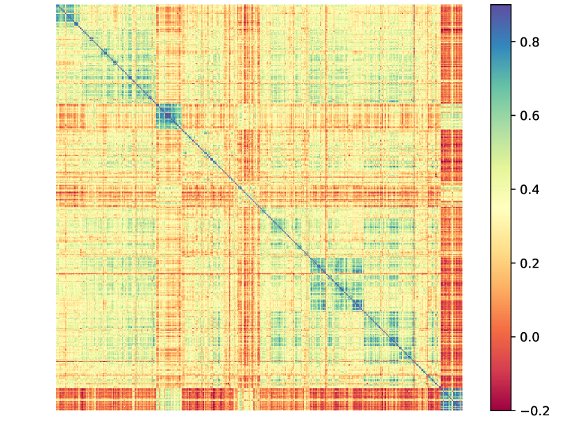
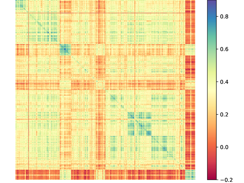
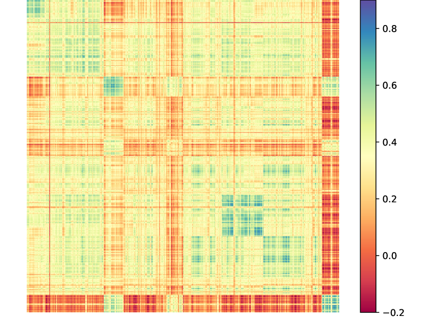
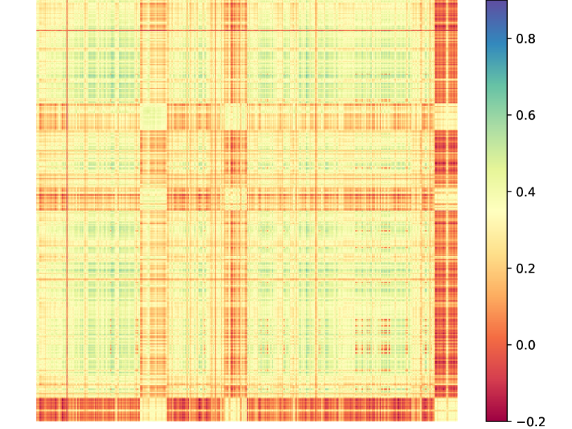
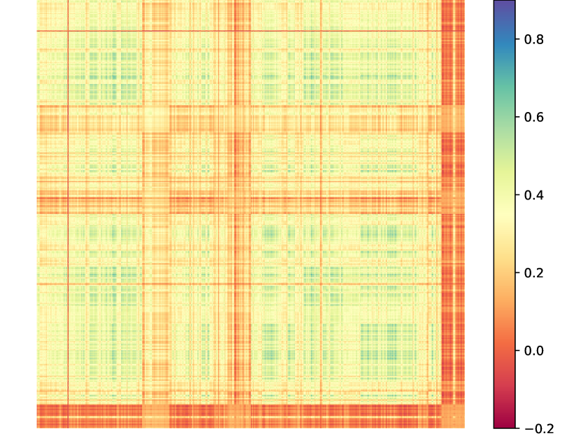
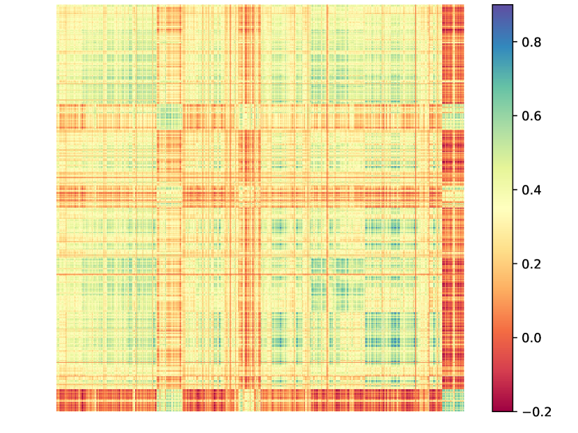
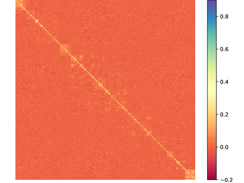
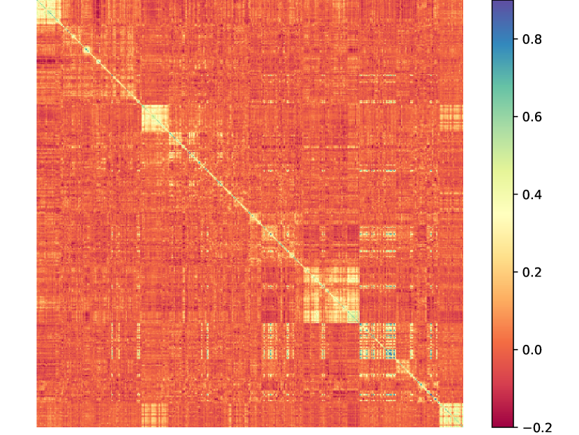
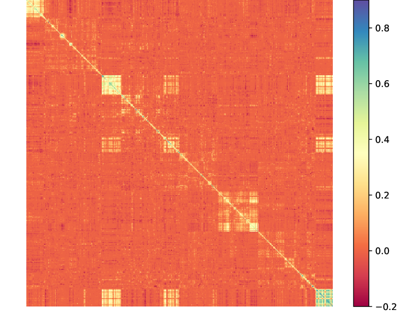
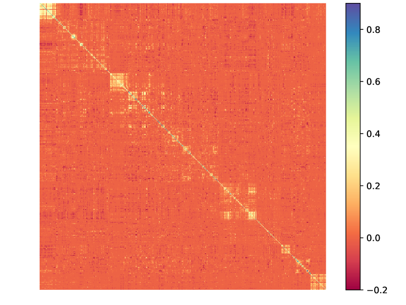
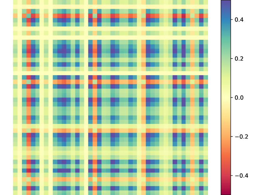
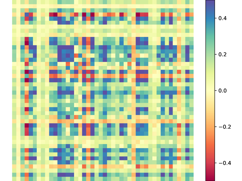
In this section, we evaluate our algorithm on real market data and compare it the other algorithms we have selected to demonstrate its capability also when the low-rank plus sparse matrix decomposition is not known. A natural candidate for our experiment is the correlation matrix of stocks in the S&P500, due to its relatively large size and the abundant, easily available data. Five hundred S&P500 stocks were part of the index between 2017 and 2018. To make the representation more readable, we have sorted these stocks in eleven sectors according to the global industry classification standard. We have constructed the correlation matrix $\Sigma$ from the daily returns of these 500 stocks during 250 consecutive trading days (see Figure 1). As the data used to construct $\Sigma$ are available at an identical frequency, the matrix $\Sigma$ is indeed positive semidefinite, with 146 eigenvalues larger than $10^{-10}$. The 70 largest eigenvalues account for 90% of $\Sigma$’s trace, that is, the sum of all its 500 eigenvalues.

In Figure 1, we display the resulting matrices $L$ and $S$ for all algorithms with respect to the same input $\Sigma$. In our method and in RPCA-GD, we have set the rank of $L$ to $k=3$. Coincidentally, we have also obtained a rank of $3$ with FPCP. Among the three output matrices $L$, the one returned by our method matches the input more closely as it contains more relevant eigenspaces. The other algorithms have transferred this information to the sparse matrix $S$. Note that the scale of values for the correlation matrix ranges between $-0.2$ and $0.9$. The ranks of $L$ obtained with the two other algorithms are $61$ for IALM and $5$ for Non-Convex RPCA, showing the difficulty of tuning these methods to obtain some desired rank. The matrix $S$ from DNN would normally be slightly less sparse than the matrix $S$ of FPCP, as FPCP applies shrinkage. However, for visualization and comparison purposes, shrinkage is also applied on $S$ returned by DNN algorithm in Figure 1.

$\Sigma$

$\Sigma$

$\Sigma$

$\Sigma$

$\Sigma$

$L$ (IALM)

$L$ (NC-RCPA)

$L$ (RPCA-GD)

$L$ (FPCP)

$L$ (DNN)

$S$ (IALM)

$S$ (NC-RCPA)

$S$ (RPCA-GD)

$S$ (FPCP)

   $S$ (DNN),        with shrinkage

Figure 1: Decomposition into a low-rank plus a sparse matrix of the correlation matrix of 500 stocks among the S&P500 stocks. The forced rank is set to $k=3$. For fair comparison with FPCP, shrinkage is applied on $S$ returned by the DNN algorithm. The obtained rank of the matrix $L$ are 61 for IALM, 5 for NC-RPCA, and 3 for the three other methods. We have $||\Sigma-L||_{F}/||L||_{F}$ at $0.16$ for DNN, and at $0.24$ for FPCP. The matrix $S$ has sparsity $0.69$ for DNN and $0.63$ for FPCP. The relative error of $L+S$ compared to $\Sigma$, where $S$ is subject to a shrinkage, is $0.076$ for DNN and $0.079$ for FPCP. When shrinkage is not applied, this error drops to $2.3\cdot 10^{-8}$ for DNN.

III-C Application on real estate return

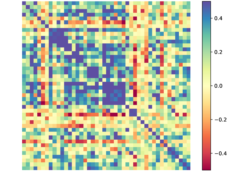
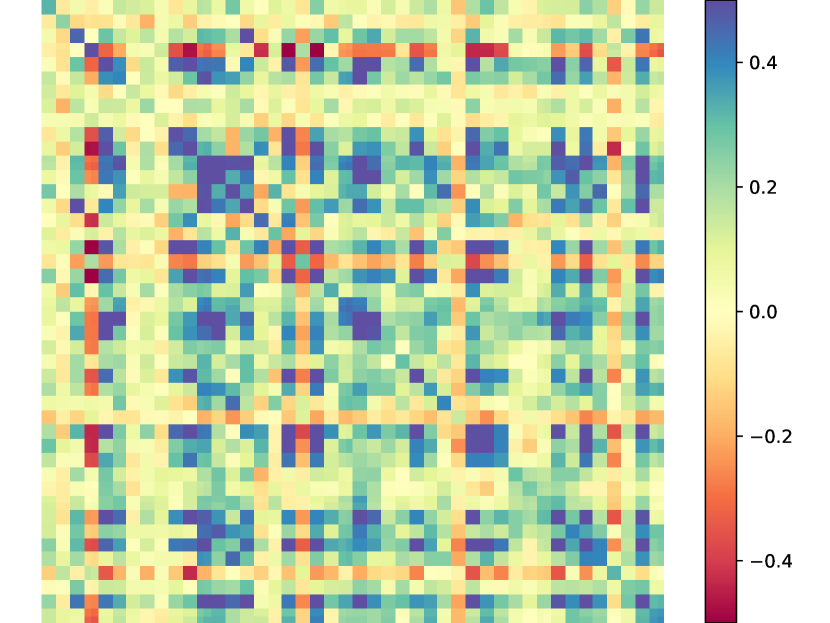
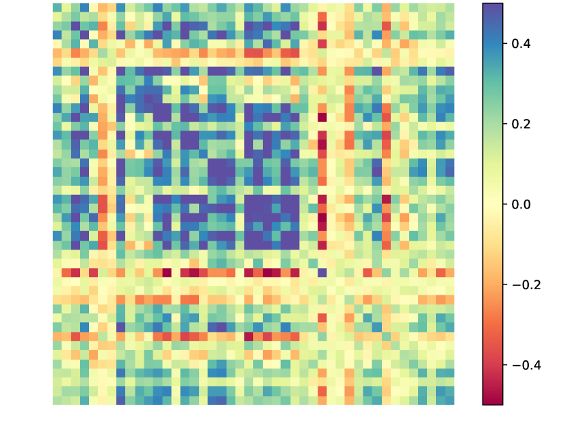
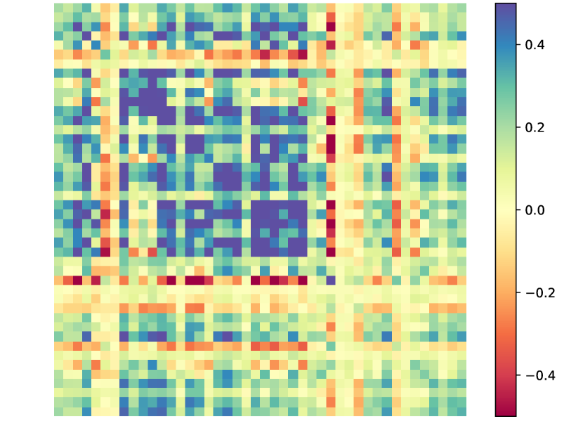
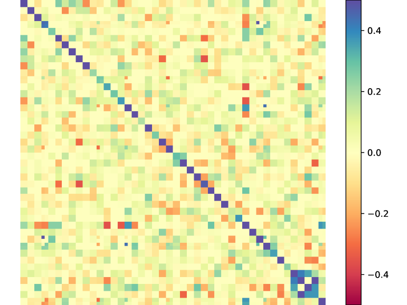
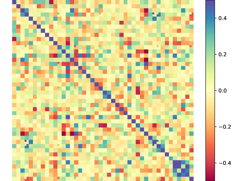
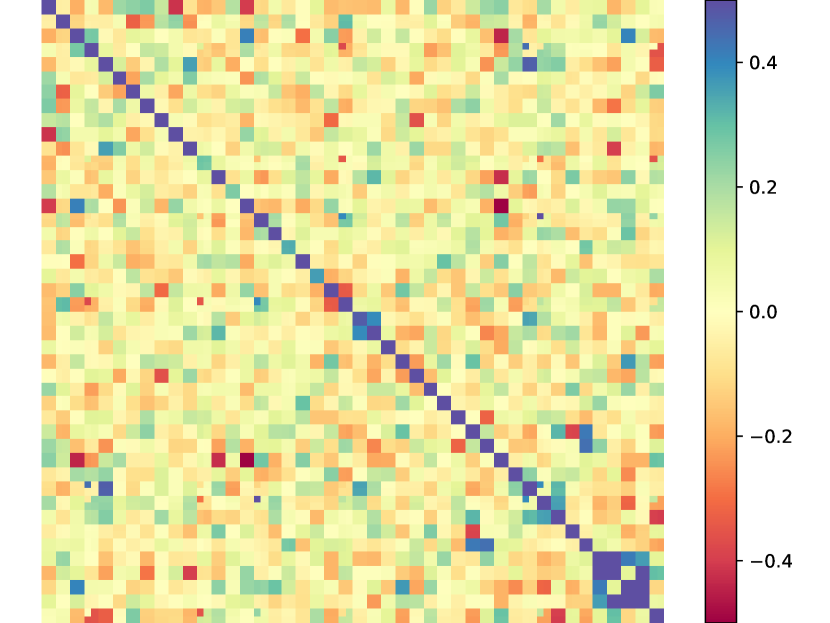
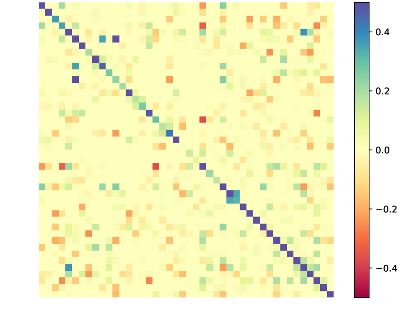
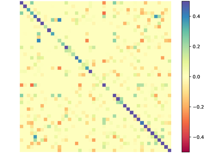
We have computed the low-rank plus sparse decomposition of the real estate return matrix for $44$ countries. The correlation matrix contains $88$ returns, alternating the residential returns and the corporate returns of each country; see Figure 2. We impose the rank of the output matrix to be equal to $3$. Similar to the previous section, the correlation color scale in Figure 2 is cropped between $-0.5$ and $0.5$ for a better visualization. The sparse matrix of FPCP is normally sparser than the one returned by our DNN algorithm. However in Figure 2, and for a fair comparison, shrinkage is also applied to the matrix $S$ returned by our algorithm. The low-rank matrices $L$ exhibit a variety of ranks from low (1 for NC-RPCA) to high (14 for IALM), indicating the difficulty of tuning the hyperparameters of these methods to a desired rank.

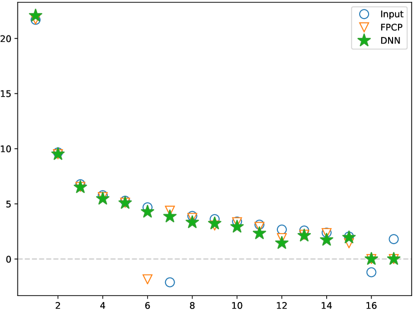
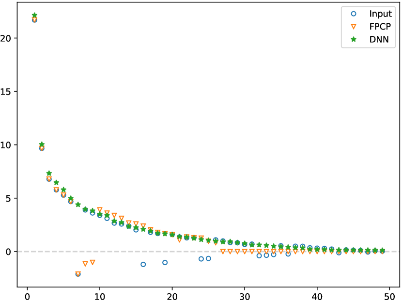
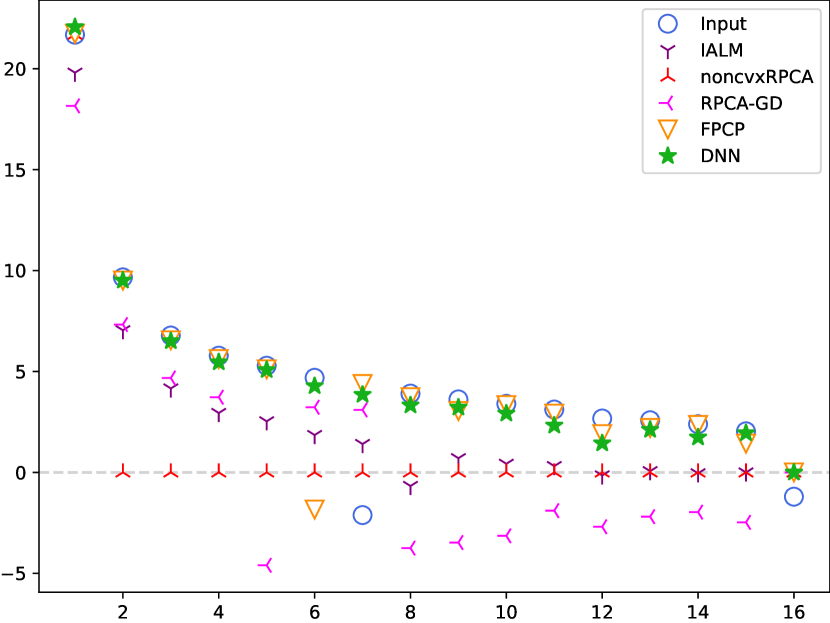
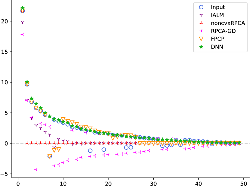
In Figure 3, we plot in the first line the eigenvalues of the matrix $L$ returned by FPCP and DNN, as well as the eigenvalues of the original matrix $\Sigma$, and for all the algorithms simultaneously in the second line. In the left figure, we display the first $17$ eigenvalues of the matrix $L$ where the forced rank is set to $k=15$. In the right figure, we plot the first $50$ eigenvalues where the forced rank is set to $k=88$. Notice that the input matrix $\Sigma$ has some negative eigenvalues. This phenomenon can happen in empirical correlation matrices when the data of the different variables are either not sampled over the same time frame or not with the same frequency; we refer to [11] for a further discussion on this issue. Our DNN algorithm and RPCA-GD, by setting $L:=MM^{T}$, avoid negative eigenvalues, although the original matrix $\Sigma$ is not positive semidefinite. In contrast, the other algorithms might output a non-positive semidefinite matrix.

$\Sigma$

$\Sigma$

$\Sigma$

$\Sigma$

$\Sigma$

$L$ (IALM)

$L$ (NC-RPCA)

$L$ (RPCA-GD)

$L$ (FPCP)

      $L$ (DNN)        

$S$ (IALM)

$S$ (NC-RPCA)

$S$ (RPCA-GD)

$S$ (FPCP)

      $S$ (DNN),         with shrinkage

Figure 2: Decomposition into a low-rank plus a sparse matrix of the correlation matrix of the real estate returns. The forced rank is set to $k=3$ for DNN and RCPA-GD. The matrix $L$ returned by FPCP has also a rank equal to $3$, while IALM gets a rank of 14 and Non-Convex RPCA gets a rank equal to 1. The relative error of $L$ compared to $\Sigma$ is $0.41$ for DNN and $0.41$ for FPCP. The sparsity of $S$ is $0.65$ for FPCP and $0.76$ for DNN with shrinkage, $0.17$ without shrinkage. The relative error of $L+S$ compared to $\Sigma$ is $0.13$ for DNN and $0.24$ for FPCP. When shrinkage is not applied, this error drops down to $2.4\cdot 10^{-8}$ with our algorithm.

Figure 3: The first 17 (left panels) and 50 (right panels) eigenvalues of the correlation matrix of the real estate returns $\Sigma$ and of the low-rank matrix $L$ outputted. The forced rank is set to $k=15$ (left) and to $k=88$ (right). For clarity, the first line compares our algorithm to FPCP only, while the second line compares all the algorithms.

III-D Empirical verification of bounded parameters

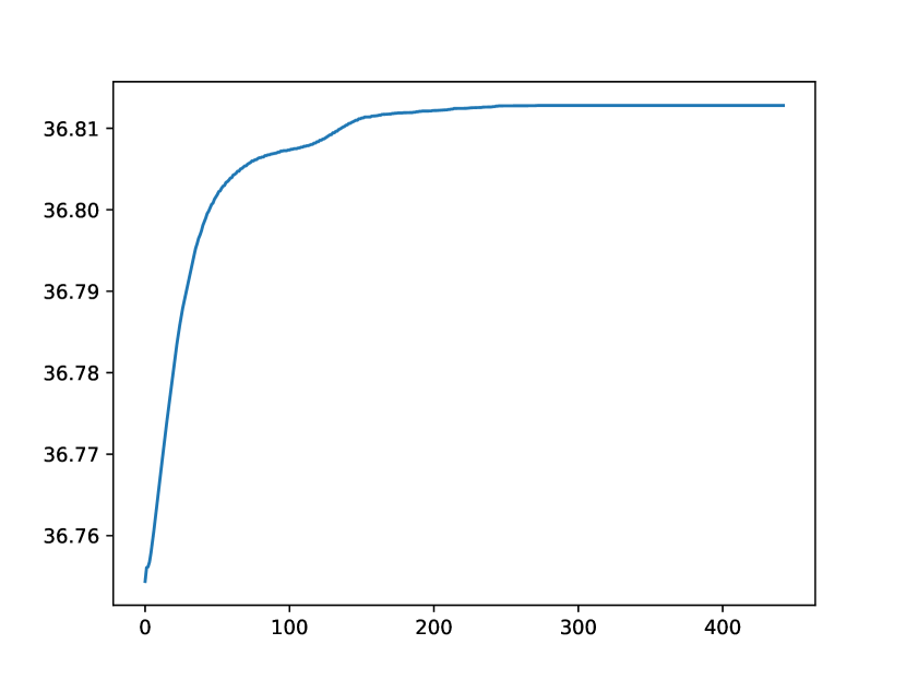
To verify empirically our assumption (12) in Theorem II.1 that the parameters $(\Theta_{j})_{j\in\mathbb{N}_{0}}$ generated by our algorithm (10) remain in a compact set, we plotted in Figure 4 the running maximum $\max_{0\leq j\leq J}\|\Theta_{j}\|$ as a function of the number of iterations $J$ for both examples on the S&P500 and the real estate data used in the previous section. For both cases, we observe, as desired, that the running maximum $\max_{0\leq j\leq J}\|\Theta_{j}\|$ converges, which means that at least empirically, $(\Theta_{j})_{j\in\mathbb{N}_{0}}$ remains in a compact set.

Figure 4: The running maximum $\max_{0\leq j\leq J}\|\Theta_{j}\|$ (y-axis) of our parameters $(\Theta_{j})_{j\in\mathbb{N}_{0}}$ generated by our DNN algorithm, plotted as a function of iterations $J$ (x-axis) for both examples on the S&P500 stock prices (left) and on the real estate returns (right).

IV Proof of convergence

A vast majority of first-order methods for minimizing locally a non-convex function with provable convergence rate are meant to minimize $L$-smooth functions, that is, differentiable functions with a Lipschitz continuous gradient. Also, the value of the Lipschitz constant with respect to a suitable norm plays a prominent role in this convergence rate (see [8] and references therein). As a critical step in the convergence proof for the minimization procedure of the function ${\varphi}$, we compute carefully a bound on the Lipschitz constant of its gradient, also called the smoothness constant below.

For establishing this bound, we use in a critical way the recursive compositional nature of the neural network that represents $M$: we first consider the case of a neural network with a single layer. We compute explicitly the derivative of the corresponding objective function $\varphi(\Theta)$ with respect to each parameter in Lemmas IV.1 and IV.2. Then, using an elementary lemma on the smoothness constant of a composition and a product of functions, we carefully derive an upper bound on the derivative of a single-layered network output with respect to the bias on the input in Lemma IV.4. This result represents the key element of our proof. Lemma IV.5 completes the picture by computing such a bound for derivatives with respect to other coefficients. Lemma IV.6 merges these results and provides a bound on the overall smoothness constant for the case where $M$ is parametrized by a single-layer neural network. Finally, we deduce inductively a bound on this Lipschitz constant for a multi-layered neural network in the proof of Theorem II.1.

So, we consider in the beginning of this section a neural network with a single layer of $\ell$ neurons. These neurons have each $\sigma:\mathbb{R}\to[-1,1]$ as activation function, and $\sigma$ has its first and the second derivative uniformly bounded by $\sigma^{\prime}_{\textrm{max}}>0$ and $\sigma^{\prime\prime}_{\textrm{max}}$, respectively. We let $r:=n(n+1)/2$, $A=\left[A_{i,j}\right]_{i,j}\in\mathbb{R}^{\ell\times r}$ be the weights, and $b=\left[b_{i}\right]_{i}\in\mathbb{R}^{\ell}$ be the bias on the input, and let

$$f_{1}^{A,b}:\mathbb{R}^{r}\to\mathbb{R^{\ell}},\qquad w\mapsto f_{1}^{A,b}(w)=Aw+b.$$

The coefficients on the output are denoted by $C=\left[C_{i,j}\right]_{i,j}\in\mathbb{R}^{nk\times\ell}$ and the bias by $d=\left[d_{i}\right]_{i}\in\mathbb{R}^{nk}$. As above, we define

$$f_{2}^{C,d}:\mathbb{R}^{\ell}\to\mathbb{R}^{nk}\qquad v\mapsto f_{2}^{C,d}(v)=Cv+d.$$

With $\tilde{\sigma}:\mathbb{R}^{\ell}\to\mathbb{R}^{\ell}$, $u\mapsto\tilde{\sigma}(u)=\left(\sigma(u_{1})\cdots\sigma(u_{\ell})\right)^{T}$, and $\Theta:=(A,b,C,d)$ the single layer neural network $\mathcal{N}^{\Theta}:\mathbb{R}^{r}\to\mathbb{R}^{nk}$ is then the composition of these three functions, that is: $\mathcal{N}^{\Theta}=f_{2}^{C,d}\circ\tilde{\sigma}\circ f_{1}^{A,b}$. For a given $\Sigma\in\mathbb{S}^{n}$, our approximated objective function with respect to the above single-layer neural network is defined by

$$\tilde{\varphi}(\Theta)=\sum_{i,j=1}^{n}\mu\left(\left[g\left(\mathcal{N}^{\Theta}\left(h(\Sigma)\right)\right)g\left(\mathcal{N}^{\Theta}\left(h(\Sigma)\right)\right)^{T}-\Sigma\right]_{i,j}\right),$$ (15)

where $\mu:\mathbb{R}\to\mathbb{R}$ is a smooth approximation of the absolute value function with a derivative uniformly bounded by $1$ and its second derivative bounded by $\mu^{\prime\prime}_{\max}$.

As announced above, we start our proof by computing the partial derivatives of $\tilde{\varphi}$. For abbreviating some lengthy expressions, we use the following shorthand notation throughout this section. We fix $\Sigma\in\mathbb{S}^{n}$ and let for $1\leq i,j\leq n$,

$$\begin{split}\omega_{i,j}&\!:=\!\left[g\left(\mathcal{N}^{\Theta}\left(h(\Sigma)\right)\right)g\left(\mathcal{N}^{\Theta}\left(h(\Sigma)\right)\right)^{T}-\Sigma\right]_{i,j}\!,\\ X&:=\mathcal{N}^{\Theta}\left(h(\Sigma)\right)\in\mathbb{R}^{nk},\\ Y&:=\tilde{\sigma}\circ f_{1}^{A,b}(h(\Sigma))\in\mathbb{R}^{\ell},\\ Z&:=f_{1}^{A,b}(h(\Sigma))\in\mathbb{R}^{\ell}.\end{split}$$ (16)

Lemma IV.1.

Let $\tilde{\varphi}$ be the function defined in (15) and $1\leq\iota\leq\ell$. Then

$$\begin{split}\frac{\partial\tilde{\varphi}(\Theta)}{\partial b_{\iota}}=\!\sum_{i,j=1}^{n}&\!\mu^{\prime}(\omega_{i,j})\sigma^{\prime}(\!Z_{\iota}\!)\times\\ &\left(\sum_{s=1}^{k}\!\left(C_{(i-1)k+s,\iota}X_{(j-1)k+s}\!+\!X_{(i-1)k+s}C_{(j-1)k+s,\iota}\!\right)\right).\end{split}$$

Moreover, for every $1\leq\iota\leq\ell$, $1\leq\eta\leq r$ we have

$$\frac{\partial\tilde{\varphi}(\Theta)}{\partial A_{\iota,\eta}}=[h(\Sigma)]_{\eta}\frac{\partial\tilde{\varphi}(\Theta)}{\partial b_{\iota}}.$$

Proof.

Let $1\leq\iota\leq\ell$. By definition of $\tilde{\varphi}$, we have

$$\begin{split}\frac{\partial\tilde{\varphi}(\Theta)}{\partial b_{\iota}}&=\sum_{i,j=1}^{n}\mu^{\prime}(\omega_{i,j})\Bigg{(}\Bigg{[}\tfrac{\partial g\left(\mathcal{N}^{\Theta}\left(h(\Sigma)\right)\right)}{\partial b_{\iota}}g\left(\mathcal{N}^{\Theta}\left(h(\Sigma)\right)\right)^{T}\\ &\qquad\qquad\qquad\quad+g\left(\mathcal{N}^{\Theta}\left(h(\Sigma)\right)\right)\tfrac{\partial g\left(\mathcal{N}^{\Theta}\left(h(\Sigma)\right)\right)^{T}}{\partial b_{\iota}}\Bigg{]}_{i,j}\Bigg{)}.\end{split}$$ (17)

As $\mathcal{N}^{\Theta}\equiv f_{2}^{C,d}\circ\tilde{\sigma}\circ f_{1}^{A,b}$, we have

$$\tfrac{\partial g\left(\mathcal{N}^{\Theta}\left(h(\Sigma)\right)\right)}{\partial b_{\iota}}=\nabla_{X}g(X)\cdot\nabla_{Z}\left(f_{2}^{C,d}\circ\tilde{\sigma}\right)(Z)\cdot\frac{\partial f_{1}^{A,b}(h(\Sigma))}{\partial b_{\iota}}.$$ (18)

Observe that

$$\frac{\partial f_{1}^{A,b}(h(\Sigma))}{\partial b_{\iota}} = \frac{\partial(Ah(\Sigma)+b)}{\partial b_{\iota}}=\left(\begin{array}[]{c}1_{\iota=1}\\ \vdots\\ 1_{\iota=\ell}\end{array}\right),$$ (22)

$$\left[\nabla_{Z}\left(f_{2}^{C,d}\circ\tilde{\sigma}\right)(Z)\right]_{\iota} = \left[\nabla_{Z}\left(C\tilde{\sigma}(Z)+d\right)\right]_{\iota}=\begin{pmatrix}C_{1,\iota}\sigma^{\prime}(Z_{\iota})\\ \vdots\\ C_{nk,\iota}\sigma^{\prime}(Z_{\iota})\end{pmatrix}.$$

The third order tensor $\nabla_{X}g(X)$, as an $nk$-dimensional vector of $n$-by-$k$ matrices, has for $((i-1)k+j)$-th element the matrix whose only nonzero element is a $1$ at position $(i,j)$, namely

$$\left[\nabla_{X}g(X)\right]_{(i-1)k+j}=\begin{pmatrix}0&\cdots&0\\ \vdots&1_{(i,j)}&\vdots\\ 0&\cdots&0\end{pmatrix}\in\mathbb{R}^{n\times k}.$$ (23)

Plugging these in (18), we get

$$\begin{split}\frac{\partial g\left(\mathcal{N}^{\Theta}\left(h(\Sigma)\right)\right)}{\partial b_{\iota}}=\sigma^{\prime}(Z_{\iota})\begin{pmatrix}C_{1,\iota}&\cdots&C_{k,\iota}\\ \vdots&&\vdots\\ C_{(n-1)k+1,\iota}&\cdots&C_{nk,\iota}\end{pmatrix},\end{split}$$

so that $\frac{\partial}{\partial b_{\iota}}\tilde{\varphi}(\Theta)$ equals

$$\sum_{i,j=1}^{n}\mu^{\prime}(\omega_{i,j})\sigma^{\prime}(Z_{\iota})\times$$

$$\quad\ \cdot\left(\left[\begin{pmatrix}C_{1,\iota}&\cdots&C_{k,\iota}\\ \vdots&&\vdots\\ C_{(n-1)k+1,\iota}&\cdots&C_{nk,\iota}\end{pmatrix}\begin{pmatrix}X_{{}_{1}}&\cdots&X_{(n-1)k+1}\\ \vdots&&\vdots\\ X_{k}&\cdots&X_{nk}\end{pmatrix}\right]_{i,j}\right.$$

$$\quad\;\;\underbrace{\;\;\ +\left.\left[\begin{pmatrix}X_{{}_{1}}&\cdots&X_{k}\\ \vdots&&\vdots\\ X_{(n-1)k+1}&\cdots&X_{nk}\end{pmatrix}\begin{pmatrix}C_{1,\iota}&\cdots&C_{(n-1)k+1,\iota}\\ \vdots&&\vdots\\ C_{k,\iota}&\cdots&C_{nk,\iota}\end{pmatrix}\right]_{i,j}\right)}_{\displaystyle\sum_{s=1}^{k}C_{(i-1)k+s,\iota}X_{(j-1)k+s}+X_{(i-1)k+s}C_{(j-1)k+s,\iota}},$$

and the first part is proved. For the second part, note that for every $1\leq\eta\leq r$ we have

$$\frac{\partial f_{1}^{A,b}(h(\Sigma))}{\partial A_{\iota,\eta}}=\frac{\partial(Ah(\Sigma)+b)}{\partial A_{\iota,\eta}}=\left(\begin{array}[]{c}[h(\Sigma)]_{\eta}1_{\iota=1}\\ \vdots\\ \left[h(\Sigma)\right]_{\eta}1_{\iota=\ell}\end{array}\right),$$ (24)

which coincides with $[h(\Sigma)]_{\eta}\frac{\partial f_{1}^{A,b}(h(\Sigma))}{\partial b_{\iota}}$ by (22). Hence, using the same derivations as in (17) and (18), we get

$$\frac{\partial\tilde{\varphi}(\Theta)}{\partial A_{\iota,\eta}}=[h(\Sigma)]_{\eta}\frac{\partial\tilde{\varphi}(\Theta)}{\partial b_{\iota}}.$$

∎

Lemma IV.2.

Let $\tilde{\varphi}$ be the function defined in (15), fix $1\leq\alpha\leq n$ and $1\leq\beta\leq k$, and set $\nu:=(\alpha-1)k+\beta$. Then

$$\frac{\partial\tilde{\varphi}(\Theta)}{\partial d_{\nu}}=2\sum_{j=1}^{n}\mu^{\prime}(\omega_{\alpha,j})X_{(j-1)k+\beta}.$$ (25)

Moreover, for every $1\leq\iota\leq\ell$, we have

$$\frac{\partial\tilde{\varphi}(\Theta)}{\partial C_{\nu,\iota}}=Y_{\iota}\frac{\partial\tilde{\varphi}(\Theta)}{\partial d_{\nu}}.$$

Proof.

Note that $\frac{\partial\tilde{\varphi}(\Theta)}{\partial d_{\nu}}$ equals

$$\sum_{i,j=1}^{n}\mu^{\prime}(\omega_{i,j})\left[\tfrac{\partial g\left(f_{2}^{C,d}(Y)\right)}{\partial d_{\nu}}g\left(X\right)^{T}+g\left(X\right)\left(\tfrac{\partial g\left(f_{2}^{C,d}(Y)\right)^{T}}{\partial d_{\nu}}\right)\right]_{i,j}.$$ (26)

As $\nu=(\alpha-1)k+\beta$, the same calculation as in (22) and (23) ensures that

$$\begin{split}\frac{\partial g\left(f_{2}^{C,d}(Y)\right)}{\partial d_{\nu}}&=\left[\nabla_{X}g(X)\right]\frac{\partial\left(CY+d\right)}{\partial d_{\nu}}\\ &=\left[\nabla_{X}g(X)\right]\left(\begin{array}[]{c}1_{\nu=1}\\ \vdots\\ 1_{\nu=nk}\end{array}\right)=\begin{pmatrix}0&\cdots&0\\ \vdots&1_{(\alpha,\beta)}&\vdots\\ 0&\cdots&0\end{pmatrix},\end{split}$$

which is a $n$-by-$k$ matrix. Hence, $\frac{\partial\tilde{\varphi}(\Theta)}{\partial d_{\nu}}$ equals

$$\sum_{i,j=1}^{n}\mu^{\prime}(\omega_{i,j})\times$$

$$\quad\quad\quad\quad\left[\begin{pmatrix}0&\cdots&0\\ \vdots&1_{(\alpha,\beta)}&\vdots\\ 0&\cdots&0\end{pmatrix}\begin{pmatrix}X_{{}_{1}}&\cdots&X_{(n-1)k+1}\\ \vdots&&\vdots\\ X_{k}&\cdots&X_{nk}\end{pmatrix}\right.$$

$$\quad\quad\quad\quad\quad\left.+\begin{pmatrix}X_{{}_{1}}&\cdots&X_{k}\\ \vdots&&\vdots\\ X_{(n-1)k+1}&\cdots&X_{nk}\end{pmatrix}\begin{pmatrix}0&\cdots&0\\ \vdots&1_{(\beta,\alpha)}&\vdots\\ 0&\cdots&0\end{pmatrix}\right]_{i,j}$$

$$=\sum_{i,j=1}^{n}\mu^{\prime}(\omega_{i,j})\times$$

$$\quad\left[\underbrace{\begin{pmatrix}0&\cdots&0\\ X_{\beta}&\cdots&X_{(n-1)k+\beta}\\ 0&\cdots&0\end{pmatrix}}_{\textrm{line}\;\alpha}+\underbrace{\begin{pmatrix}0&\cdots&X_{\beta}&\cdots&0\\ \vdots&&\vdots&&\vdots\\ 0&\cdots&X_{(n-1)k+\beta}&\cdots&0\end{pmatrix}}_{\textrm{column}\;\alpha}\right]_{i,j}.$$

Since $\omega_{i,j}=\omega_{j,i}$ for every $1\leq i,j\leq n$ we finally get

$$\frac{\partial\tilde{\varphi}(\Theta)}{\partial d_{\nu}} = 2\mu^{\prime}\!(\omega_{\alpha,\alpha}\!)X_{(\alpha-1)k+\beta}$$

$$+\sum_{\begin{subarray}{c}j=1\\ j\neq\alpha\end{subarray}}^{n}\mu^{\prime}\!(\omega_{\alpha,j}\!)X_{(j-1)k+\beta}\!+\!\sum_{\begin{subarray}{c}i=1\\ i\neq\alpha\end{subarray}}^{n}\mu^{\prime}\!(\omega_{i,\alpha}\!)X_{(i-1)k+\beta}$$

$$= 2\sum_{j=1}^{n}\mu^{\prime}(\omega_{\alpha,j})X_{(j-1)k+\beta},$$

which proves the first part. For the second part, we fix $1\leq\iota\leq\ell$. In the same manner as we established (24), we can use (23) to see that

$$\frac{\partial g\left(f_{2}^{C,d}(Y)\right)}{\partial C_{\nu,\iota}}=[\nabla_{X}g(X)]\frac{\partial(CY+d)}{\partial C_{\nu,\iota}}$$

$$= [\nabla_{X}g(X)]Y_{\iota}\left(\begin{array}[]{c}1_{\nu=1}\\ \vdots\\ 1_{\nu=nk}\end{array}\right)=Y_{\iota}\frac{\partial g\left(f_{2}^{C,d}(Y)\right)}{\partial b_{\nu}},$$

and thereby, with (26), to conclude that

$$\frac{\partial\tilde{\varphi}(\Theta)}{\partial C_{\nu,\iota}}=Y_{\iota}\frac{\partial\tilde{\varphi}(\Theta)}{\partial d_{\nu}}.$$

∎

One of the key tools in the derivation of bounds on the Lipschitz constant of $\tilde{\varphi}$ is the following elementary lemma. It shows how to infer the Lipschitz constant of some functions from the Lipschitz constant of other, simpler Lipschitz-continuous functions.

Lemma IV.3.

Let $\phi_{1}:\mathbb{R}^{m}\to\mathbb{R}$ be Lipschitz continuous with Lipschitz constant $L_{1}$. Let $\phi_{2}:\mathbb{R}^{n}\to\mathbb{R}^{m}$ be a function for which there exists a some $L_{2}:\mathbb{R}^{n}\times\mathbb{R}^{n}\to(0,\infty)$ such that for all $x,y\in\mathbb{R}^{n}$ we have

$$\|\phi_{2}(x)-\phi_{2}(y)\|\leq L_{2}(x,y)\|x-y\|.$$ (28)

Assume that $\phi_{1}\circ\phi_{2}$ is bounded by a constant $B_{12}$. Finally, let $\phi_{3}:\mathbb{R}^{n}\to\mathbb{R}$ be a function for which

1. $|\phi_{3}(y)|\leq B_{3}(y)$ for all $y\in\mathbb{R}^{n}$ for some positive function $B_{3}\colon\mathbb{R}^{n}\to(0,\infty)$;

2. there exist three functions $L_{31}:\mathbb{R}^{n}\times\mathbb{R}^{n}\to(0,\infty)$, $L_{32}:\mathbb{R}^{n}\times\mathbb{R}^{n}\to(0,\infty)$, and $f:\mathbb{R}^{n}\to\mathbb{R}^{p}$ such that for all $x,y\in\mathbb{R}^{n}$ we have

   $$\|\phi_{3}(x)-\phi_{3}(y)\|\leq L_{31}(x,y)\|x-y\|+L_{32}(x,y)\|f(x)-f(y)\|.$$

Then, for every $x,y\in\mathbb{R}^{n}$, the function $\Phi:=(\phi_{1}\circ\phi_{2})\phi_{3}$ verifies

$$|\Phi(x)-\Phi(y)| \leq \left(B_{12}L_{31}(x,y)+B_{3}(y)L_{1}L_{2}(x,y)\right)\|x-y\|$$

$$+B_{12}L_{32}(x,y)\|f(x)-f(y)\|.$$

Proof.

For all $x,y\in\mathbb{R}^{n}$, we can write

$$\begin{split}&|\Phi(x)-\Phi(y)|=\left|\phi_{1}\left(\phi_{2}(x)\right)\phi_{3}(x)-\phi_{1}\left(\phi_{2}(y)\right)\phi_{3}(y)\right|\\ &\leq\left|\phi_{1}\left(\phi_{2}(x)\right)\left(\phi_{3}(x)-\phi_{3}(y)\right)\right|+\left|\left(\phi_{1}\left(\phi_{2}(x)\right)-\phi_{1}\left(\phi_{2}(y)\right)\right)\phi_{3}(y)\right|\\ &\leq B_{12}\left|\phi_{3}(x)-\phi_{3}(y)\right|+B_{3}(y)\left|\phi_{1}\left(\phi_{2}(x)\right)-\phi_{1}\left(\phi_{2}(y)\right)\right|\\ &\leq B_{12}\big{(}L_{31}(x,y)\|x\!-\!y\|\!+\!L_{32}(x,y)\|f(x)\!-\!f(y)\|\big{)}\\ &\quad+\!B_{3}L_{1}\left\|\phi_{2}(x)\!-\!\phi_{2}(y)\right\|.\end{split}$$

It remains to use (28) on the last term to conclude. ∎

As defined in (11), the norm we use for a finite list of matrix of different sizes is the Euclidean norm of the vector constituted by their Frobenius norms. For symmetric matrices $X$, we also use a dedicated norm defined as $||X||_{S}:=||h(X)||$, where $h:\mathbb{S}^{n}\to\mathbb{R}^{n(n+1)/2}$ is the function defined in (8). Note also that $2||X||_{S}^{2}=||X||_{F}^{2}+||\textrm{diag}(X)||_{F}^{2}$.

The next lemma is a key step in determining a bound on the smoothness constant of our objective function $\tilde{\varphi}$.

Lemma IV.4.

Let $\tilde{\varphi}$ be the function defined in (15) and let $D>0$ be any constant. We define

$$\mathcal{D}:=\big{\{}(A,b,C,d)\in\mathbb{R}^{l\times r}\times\mathbb{R}^{\ell}\times\mathbb{R}^{nk\times\ell}\times\mathbb{R}^{nk}\colon\|(A,b,C,d)\|\leq D\big{\}}.$$

The function

$$\Theta=(A,d,C,d)\mapsto\frac{\partial\tilde{\varphi}(\Theta)}{\partial b}\in\mathbb{R}^{\ell}$$

is Lipschitz continuous on $\mathcal{D}$ with a constant $L_{b}$ for which

$$L^{2}_{b}=\mathcal{C}_{b}n^{2}D^{2}\max\!\left\{\ell D^{2}L^{2}_{Z},\ell^{2}D^{6}L_{Z}^{2},\ell^{3}D^{4},n\ell\right\},$$

where $L_{Z}:=\sqrt{1+\|\Sigma\|_{S}^{2}}$ and $\mathcal{C}_{b}$ is a constant that only depends polynomially on $\sigma^{\prime}_{\max},\sigma^{\prime\prime}_{\max},\mu^{\prime\prime}_{\max}$.

Proof.

We divide the proof into several steps, each of which establishing that some function is bounded and/or Lipschitz continuous. We set $\Theta=(A,b,C,d)$ and $\bar{\Theta}=(\bar{A},\bar{b},\bar{C},\bar{d})$ in $\mathcal{D}$. We make use abundantly of the shorthand notation defined in (16), adopting the notation $\bar{\omega}_{ij}$, $\bar{X}$, etc…when $\Theta$ is replaced by $\bar{\Theta}$.

Step 1. Let $1\leq\iota\leq\ell$. In this first step, we focus on $Z_{\iota}=\left[f_{1}^{A,b}(h(\Sigma))\right]_{\iota}$. The Cauchy-Schwarz Inequality ensures that for every $(A,b),(\bar{A},\bar{b})\in\mathbb{R}^{\ell\times r}\times\mathbb{R}^{\ell}$ we have

$$\begin{split}&\left(Z_{\iota}-\bar{Z}_{\iota}\right)^{2}=\Big{(}(A_{\iota,:}-\bar{A}_{\iota,:})h(\Sigma)+b_{\iota}-\bar{b}_{\iota}\Big{)}^{2}\\ &\leq\left\|\begin{array}[]{c}A_{\iota,:}-\bar{A}_{\iota,:}\\ b_{\iota}-\bar{b}_{\iota}\end{array}\right\|^{2}\left\|\begin{array}[]{c}h(\Sigma)\\ 1\end{array}\right\|^{2}=L_{Z}^{2}||({A}_{\iota,:},{b}_{\iota})-(\bar{A}_{\iota,:},\bar{b}_{\iota})||^{2}.\end{split}$$

Step 2. Let us apply Lemma IV.3 with $\phi_{1}\equiv\sigma$, $\phi_{2}\equiv\left[f_{1}^{\cdot,\cdot}(h(\Sigma))\right]_{\iota}$, and $\phi_{3}\equiv 1$. We have immediately $L_{31}=L_{32}=0$, $B_{3}=1$, $L_{1}=\sigma^{\prime}_{\max}$, and, by Step $1$, $L_{2}=L_{Z}$. Therefore,

$$\left|\sigma\left(Z_{\iota}\right)-\sigma\left(\bar{Z}_{\iota}\right)\right|\leq\sigma^{\prime}_{\max}L_{Z}||({A}_{\iota,:},{b}_{\iota})-(\bar{A}_{\iota,:},\bar{b}_{\iota})||.$$

Note also that $\|\tilde{\sigma}(\bar{Z})\|\leq\sqrt{\ell}$ because $|\sigma\left(\bar{Z}_{\iota}\right)|\leq 1$ by assumption on $\sigma$.

Step 3. Similarly, we get

$$\left|\sigma^{\prime}\left(Z_{\iota}\right)-\sigma^{\prime}\left(\bar{Z}_{\iota}\right)\right|\leq\sigma^{\prime\prime}_{\max}L_{Z}||({A}_{\iota,:},{b}_{\iota})-(\bar{A}_{\iota,:},\bar{b}_{\iota})||.$$

Also, $\sigma^{\prime}\left(Z_{\iota}\right)\leq\sigma^{\prime}_{\max}$ by assumption.

Step 4. Let us fix $1\leq\nu\leq nk$. We focus in this step on $X_{\nu}=\left[f_{2}^{{C,}{d}}\circ\tilde{\sigma}\circ f_{1}^{{A},{b}}(h(\Sigma))\right]_{\nu}=\left[f_{2}^{{C,}{d}}(Y)\right]_{\nu}$, with $Y=\tilde{\sigma}(Z)=\tilde{\sigma}\circ f_{1}^{{A},{b}}(h(\Sigma))$. Observe first that

$$\left|X_{\nu}-\bar{X}_{\nu}\right|=\left|{C}_{\nu,:}{Y}+{d}_{\nu}-\bar{C}_{\nu,:}{\bar{Y}}-\bar{d}_{\nu}\right|$$

$$\leq\sum_{\iota=1}^{\ell}{|C}_{\nu,\iota}|\cdot|Y_{\iota}-\bar{Y}_{\iota}|+\left\|C_{\nu,:}-\bar{C}_{\nu,:}\right\|\cdot\left\|\bar{Y}\right\|+\left|d_{\nu}-\bar{d}_{\nu}\right|$$

$$\leq\sum_{\iota=1}^{\ell}|{C}_{\nu,\iota}|\sigma^{\prime}_{\max}L_{Z}\cdot\left\|\begin{array}[]{c}A_{\iota,:}-\bar{A}_{\iota,:}\\ b_{\iota}-\bar{b}_{\iota}\end{array}\right\|$$

$$\;\;+\left\|C_{\nu,:}-\bar{C}_{\nu,:}\right\|\left\|\bar{Y}\right\|+\left|d_{\nu}-\bar{d}_{\nu}\right|\qquad\textrm{(by Step $2$).}$$

Squaring both sides of this inequality and using Cauchy-Schwarz, we get

$$\left(X_{\nu}-\bar{X}_{\nu}\right)^{2}$$

$$\leq\left(\left(\sum_{\iota=1}^{\ell}{C}_{\nu,\iota}^{2}\right)\left(\sigma^{\prime}_{\max}\right)^{2}L_{Z}^{2}+||\bar{Y}||^{2}+1\right)\times$$

$$\;\;\;\;\;\;\Big{(}||A-\bar{A}||^{2}+||b-\bar{b}||^{2}+||C_{\nu,:}-\bar{C}_{\nu,:}||^{2}+\left|d_{\nu}-\bar{d}_{\nu}\right|^{2}\Big{)}$$

$$\leq L^{2}_{\nu}\left\|(A,b,C_{\nu,:},d_{\nu})-(\bar{A},\bar{b},\bar{C}_{\nu,:},\bar{d}_{\nu})\right\|^{2}.$$ (29)

with

$$L_{\nu}^{2}:=\left(||{C}_{\nu,:}||\sigma^{\prime}_{\max}L_{Z}\right)^{2}+\ell+1.$$ (30)

This last inequality is also ensured by Step $2$, where we showed that $||\bar{Y}||\leq\sqrt{\ell}$.

In addition to providing an estimate for its Lipschitz constant, we can also obtain a bound for this function. From Step $2$, we get

$$\left|X_{\nu}\right| =\left|{C}_{\nu,:}{Y}+{d}_{\nu}\right|\leq||{C}_{\nu,:}||\sqrt{\ell}+|{d}_{\nu}|$$

$$\leq\sqrt{\ell+1}\cdot\sqrt{||{C}_{\nu,:}||^{2}+|{d}_{\nu}|^{2}}.$$ (31)

We obtain with this step the Lipschitz constant of one output of a single-layer neural network. Would our objective function be the standard least square loss function to minimize when training a neural network, the remaining of our task would have been vastly simpler. The specific intricacies of our objective function (15) ask for a more involved analysis.

Step 5. Let $1\leq i,j\leq n$. In this step, we deal with the function

$$\omega_{i,j}:=\left[g\left(X\right)g\left(X\right)^{T}-\Sigma\right]_{i,j}.$$

We have

$$\big{|}\omega_{i,j}-\bar{\omega}_{i,j}\big{|}^{2}=\left[g\left(X\right)g\left(X\right)^{T}-g\left(\bar{X}\right)g\left(\bar{X}\right)^{T}\right]^{2}_{i,j}$$

$$\leq\left(\sum_{s=1}^{k}\Big{[}\left|X_{(i-1)k+s}\right|\cdot\left|X_{(j-1)k+s}-\bar{X}_{(j-1)k+s}\right|\right.$$

$$\quad\quad\quad+\left|\bar{X}_{(j-1)k+s}\right|\cdot\left|X_{(i-1)k+s}-\bar{X}_{(i-1)k+s}\right|\Big{]}\Bigg{)}^{2}$$ (32)

$$\leq\;2\left(\sum_{s=1}^{k}X_{(i-1)k+s}^{2}\right)\cdot\left(\sum_{s=1}^{k}|X_{(j-1)k+s}-\bar{X}_{(j-1)k+s}|^{2}\right)$$

$$\quad+2\left(\sum_{s=1}^{k}\bar{X}_{(j-1)k+s}^{2}\right)\cdot\left(\sum_{s=1}^{k}|X_{(i-1)k+s}-\bar{X}_{(i-1)k+s}|^{2}\right).$$

Let us bound these four sums using (29) and (31). First,

$$\sum_{s=1}^{k}X_{(i-1)k+s}^{2}\leq(\ell+1)\left(\sum_{s=1}^{k}\left(\|C_{(i-1)k+s,:}\|^{2}+d_{(i-1)k+s}^{2}\right)\right).$$

The sum on the right-hand side can be conveniently rewritten using the vector-to-matrix operator $g$.

$$\sum_{s=1}^{k}\|C_{(i-1)k+s,:}\|^{2}=\sum_{s=1}^{k}\sum_{\iota=1}^{\ell}C_{(i-1)k+s,\iota}^{2}=\sum_{\iota=1}^{\ell}\|g(C_{:,\iota})_{i,:}\|^{2}.$$ (33)

Similarly, we can write $\sum_{s=1}^{k}\|d_{(i-1)k+s}\|^{2}=\|g(d)_{i,:}\|^{2}$, so that

$$\sum_{s=1}^{k}X_{(i-1)k+s}^{2}\leq(\ell+1)\left(\sum_{\iota=1}^{\ell}\|g(C_{:,\iota})_{i,:}\|^{2}+\|g(d)_{i,:}\|^{2}\right).$$

Second, with $\Theta_{I(\nu)}:=(A,b,C_{\nu,:},d_{\nu})$ and writing $\nu(s):=(j-1)k+s$ for $1\leq s\leq k$, we have

$$\sum_{s=1}^{k}|X_{\nu(s)}-\bar{X}_{\nu(s)}|^{2}\leq\sum_{s=1}^{k}L^{2}_{\nu(s)}\left\|\Theta_{I(\nu(s))}-\bar{\Theta}_{I(\nu(s))}\right\|^{2}.$$

We can use the crude bound

$$\sum_{s=1}^{k}\left\|\Theta_{I(\nu(s))}-\bar{\Theta}_{I(\nu(s))}\right\|^{2}\leq\left\|\Theta-\bar{\Theta}\right\|^{2}$$

to get

$$\sum_{s=1}^{k}L^{2}_{\nu(s)}\left\|\Theta_{I(\nu(s))}-\bar{\Theta}_{I(\nu(s))}\right\|^{2}$$

$$\leq\left(\left(\sigma^{\prime}_{\max}L_{Z}\right)^{2}\sum_{s=1}^{k}||{C}_{\nu(s),:}||^{2}+\ell+1\right)\left\|\Theta-\bar{\Theta}\right\|^{2}$$

$$=\left(\left(\sigma^{\prime}_{\max}L_{Z}\right)^{2}\sum_{\iota=1}^{\ell}\|g(C_{:,\iota})_{j,:}\|^{2}+\ell+1\right)\left\|\Theta-\bar{\Theta}\right\|^{2}$$

by (33). We can plug our two estimates into our bound for $|\omega_{i,j}-\bar{\omega}_{i,j}|^{2}$ to get

$$|\omega_{i,j}-\bar{\omega}_{i,j}|\leq L_{\omega,i,j}\left\|\Theta-\bar{\Theta}\right\|$$

with

$$\left.L_{\omega,i,j}^{2}\middle/\left(2\left(\ell+1\right)\left(\sigma^{\prime}_{\max}L_{Z}\right)^{2}\right)\right.$$ (34)

$$=\left(\sum_{\iota=1}^{\ell}||g({C}_{:,\iota})_{i,:}||^{2}+||g({d})_{i,:}||^{2}\right)\left(\sum_{\iota=1}^{\ell}||g({C}_{:,\iota})_{j,:}||^{2}+\kappa\right)$$

$$\;\;+\left(\sum_{\iota=1}^{\ell}||g({\bar{C}}_{:,\iota})_{j,:}||^{2}+||g(\bar{d})_{j,:}||^{2}\right)\left(\sum_{\iota=1}^{\ell}||g({C}_{:,\iota})_{i,:}||^{2}+\kappa\right),$$

where, $\kappa:=(\ell+1)/\left(\sigma^{\prime}_{\max}L_{Z}\right)^{2}$.

Step 6. In this step, we fix $1\leq i,j\leq n$ and $1\leq\iota\leq\ell$ and focus on $\mu^{\prime}\left({\omega}_{i,j}\right)\sigma^{\prime}({Z}_{\iota})$. We therefore seek to apply Lemma IV.3 with $\phi_{1}\equiv\mu^{\prime}$, $\phi_{2}\equiv{\omega}_{i,j}$, and $\phi_{3}\equiv\sigma^{\prime}({Y}_{\iota})$. The assumptions on $\mu$ allow us to take $L_{1}=\mu^{\prime\prime}_{\max}$ and $B_{12}=1$. Step $5$ shows that $L_{2}$ can be taken as $L_{\omega,i,j}$. Step $3$ allows us to pick $L_{31}=\sigma^{\prime\prime}_{\max}L_{Z}$ with $L_{32}=0$ and $B_{3}=\sigma^{\prime}_{\max}$ by our assumptions on $\sigma$.

We obtain that

$$\left|\mu^{\prime}\left({\omega}_{i,j}\right)\sigma^{\prime}({Z}_{\iota})-\mu^{\prime}\left(\bar{\omega}_{i,j}\right)\sigma^{\prime}(\bar{Z}_{\iota})\right|\\ \leq L_{\mu^{\prime}\sigma^{\prime},i,j}\|\Theta-\bar{\Theta}\|$$

with

$$L_{\mu^{\prime}\sigma^{\prime},i,j}:=\sigma^{\prime\prime}_{\max}L_{Z}+\sigma^{\prime}_{\max}\mu^{\prime\prime}_{\max}L_{\omega,i,j}.$$

Evidently, we also have $\mu^{\prime}\left({\omega}_{i,j}\right)\sigma^{\prime}({Z}_{\iota})\leq\sigma^{\prime}_{\max}$.

Step 7. The formula for $\frac{\partial\tilde{\varphi}(\Theta)}{\partial b_{\iota}}$ obtained in Lemma IV.1 appears as a weighted sum of sums. Step $6$ did focus on the weights of this combination. In this step, we deal with these sums. We fix again $1\leq i,j\leq n$ and $1\leq\iota\leq\ell$ and define

$$V_{i,j,\iota}:=\sum_{s=1}^{k}C_{(i-1)k+s,\iota}X_{(j-1)k+s}.$$

We define similarly $\bar{V}_{i,j,\iota}$ according to our usual convention to replace $\Theta$ by $\bar{\Theta}$. Using the same argument as in Step $5$, we can write

$$\big{|}V_{i,j,\iota}-\bar{V}_{i,j,\iota}\big{|}^{2}$$

$$\leq\left(\sum_{s=1}^{k}\Big{[}\left|C_{(i-1)k+s,\iota}\right|\cdot\left|X_{(j-1)k+s}-\bar{X}_{(j-1)k+s}\right|\right.$$

$$\quad\quad\quad+\left|\bar{X}_{(j-1)k+s}\right|\cdot\left|C_{(i-1)k+s,\iota}-\bar{C}_{(i-1)k+s,\iota}\right|\Big{]}\Bigg{)}^{2}$$

$$\leq\;2\left(\sum_{s=1}^{k}C_{(i-1)k+s,\iota}^{2}\right)\cdot\left(\sum_{s=1}^{k}|X_{(j-1)k+s}-\bar{X}_{(j-1)k+s}|^{2}\right)$$

$$\quad+2\left(\sum_{s=1}^{k}\bar{X}_{(j-1)k+s}^{2}\right)\cdot\left(\sum_{s=1}^{k}|C_{(i-1)k+s,\iota}-\bar{C}_{(i-1)k+s,\iota}|^{2}\right).$$

We can bound the sums involving $X$ or $\bar{X}$ as in Step $5$. The sums with $C,\bar{C}$ can we rewritten using (33); in particular,

$$\sum_{s=1}^{k}|C_{(i-1)k+s,\iota}-\bar{C}_{(i-1)k+s,\iota}|^{2}=||g(C_{:,\iota})_{i,:}-g(\bar{C}_{:,\iota})_{i,:}||^{2}.$$

We obtain

$$\big{|}V_{i,j,\iota}-\bar{V}_{i,j,\iota}\big{|}^{2}$$

$$\leq L_{CdX,i,j,\iota}^{2}\left\|\Theta-\bar{\Theta}\right\|^{2}+L_{XdC,i,j,\iota}^{2}||g(C_{:,\iota})_{i,:}-g(\bar{C}_{:,\iota})_{i,:}||^{2}.$$

with

$$L^{2}_{CdX,i,j,\iota} :=2||g({C}_{:,\iota})_{i,:}||^{2}\times$$

$$\quad\bigg{(}\left(\sigma^{\prime}_{\max}L_{Z}\right)^{2}\textstyle\sum\limits_{\jmath=1}^{\ell}||g({C}_{:,\jmath})_{j,:}||^{2}+\ell+1\bigg{)},$$

$$L_{XdC,j,\iota}^{2} :=2(\ell+1)\bigg{(}\textstyle\sum\limits_{\jmath=1}^{\ell}||g(\bar{C}_{:,\jmath})_{j,:}||^{2}+||g(\bar{d})_{j,:}||^{2}\bigg{)}.$$

We can also obtain an upper bound to $\big{|}V_{i,j,\iota}\big{|}$ due to

$$V_{i,j,\iota}^{2} \leq\left(\sum_{s=1}^{k}C_{(i-1)k+s,\iota}^{2}\right)\left(\sum_{s=1}^{k}X_{(j-1)k+s}^{2}\right)$$

$$\leq||g({C}_{:,\iota})_{i,:}||^{2}(\ell+1)\left(\sum_{\jmath=1}^{\ell}||g({C}_{:,\jmath})_{j,:}||^{2}+||g({d})_{j,:}||^{2}\right)$$

$$=:B^{2}_{CX,i,j,\iota}$$

by using Cauchy-Schwarz, (33), and a bound obtained in Step $5$.

Step 8. We start this final step by applying Lemma IV.3 to the function $\Upsilon_{i,j,\iota}:=\mu^{\prime}(\omega_{i,j})\sigma^{\prime}(Z_{\iota})\left(V_{i,j,\iota}+V_{j,i,\iota}\right)$ by taking $\phi_{1}\equiv id_{\mathbb{R}}$, $\phi_{2}\equiv\mu^{\prime}(\omega_{i,j})\sigma^{\prime}(Z_{\iota})$, and $\phi_{3}\equiv V_{i,j,\iota}+V_{j,i,\iota}$. Evidently $L_{1}=1$. In Step $6$, we have shown that we can take $B_{12}=\sigma^{\prime}_{\max}$ and $L_{2}=L_{\mu^{\prime}\sigma^{\prime},i,j}$. By Step $7$, we can set $B_{3}=B_{CX,i,j,\iota}+B_{CX,j,i,\iota}$, $L_{31}=L_{CdX,i,j,\iota}+L_{CdX,j,i,\iota}$, and $L_{32}=0$. We obtain that

$$\left|\Upsilon_{i,j,\iota}-\bar{\Upsilon}_{i,j,\iota}\right|$$

$$\leq L_{\mu^{\prime}\sigma^{\prime},i,j}\big{(}B_{CX,i,j,\iota}+B_{CX,j,i,\iota}\big{)}||\Theta-\bar{\Theta}||$$

$$\quad+\sigma^{\prime}_{\max}(L_{CdX,i,j,\iota}+L_{CdX,j,i,\iota}\big{)}||\Theta-\bar{\Theta}||$$

$$\quad+\sigma^{\prime}_{\max}\,L_{XdC,j,\iota}\,||g(C_{:,\iota})_{i,:}-g(\bar{C}_{:,\iota})_{i,:}||$$

$$\quad+\sigma^{\prime}_{\max}\,L_{XdC,i,\iota}\,||g(C_{:,\iota})_{j,:}-g(\bar{C}_{:,\iota})_{j,:}||.$$

Since in view of Lemma IV.4, $\frac{\partial\tilde{\varphi}(\Theta)}{\partial b_{\iota}}$ is the sum of $\Upsilon_{i,j,\iota}$ over $i,j$, we obtain immediately the Lipschitz continuity of this partial derivative. Squaring the above bound and using Cauchy-Schwarz on the 6-terms right-hand side, we get

$$\sum_{\iota=1}^{\ell}\left(\frac{\partial\tilde{\varphi}(\Theta)}{\partial b_{\iota}}-\frac{\partial\tilde{\varphi}(\bar{\Theta})}{\partial b_{\iota}}\right)^{2}=\sum_{\iota=1}^{\ell}\left(\sum_{i,j=1}^{n}\Upsilon_{i,j,\iota}-\bar{\Upsilon}_{i,j,\iota}\right)^{2}$$

$$\leq 6n^{2}\sum_{\iota=1}^{\ell}\sum_{i,j=1}^{n}L_{\mu^{\prime}\sigma^{\prime},i,j}^{2}B_{CX,i,j,\iota}^{2}||\Theta-\bar{\Theta}||^{2}$$

$$\quad+6n^{2}\sum_{\iota=1}^{\ell}\sum_{i,j=1}^{n}L_{\mu^{\prime}\sigma^{\prime},i,j}^{2}B_{CX,j,i,\iota}^{2}||\Theta-\bar{\Theta}||^{2}$$

$$\quad+6\left(n\sigma^{\prime}_{\max}\right)^{2}\sum_{\iota=1}^{\ell}\sum_{i,j=1}^{n}L_{CdX,i,j,\iota}^{2}||\Theta-\bar{\Theta}||^{2}$$

$$\quad+6\left(n\sigma^{\prime}_{\max}\right)^{2}\sum_{\iota=1}^{\ell}\sum_{i,j=1}^{n}L_{CdX,j,i,\iota}^{2}||\Theta-\bar{\Theta}||^{2}$$

$$\quad+6\left(n\sigma^{\prime}_{\max}\right)^{2}\sum_{\iota=1}^{\ell}\sum_{i,j=1}^{n}L_{XdC,j,\iota}^{2}||g(C_{:,\iota})_{i,:}-g(\bar{C}_{:,\iota})_{i,:}||^{2}$$

$$\quad+6\left(n\sigma^{\prime}_{\max}\right)^{2}\sum_{\iota=1}^{\ell}\sum_{i,j=1}^{n}L_{XdC,i,\iota}^{2}||g(C_{:,\iota})_{j,:}-g(\bar{C}_{:,\iota})_{j,:}||^{2}.$$

It remains to estimate these six sums. For the first one (and the second one by symmetry), we can proceed as follows.

$$\sum_{\iota=1}^{\ell}\sum_{i,j=1}^{n}L_{\mu^{\prime}\sigma^{\prime},i,j}^{2}B_{CX,i,j,\iota}^{2}$$

$$=2\left(\ell+1\right)\left(\sigma^{\prime\prime}_{\max}L_{Z}\right)^{2}\times$$

$$\qquad\sum_{\iota=1}^{\ell}\sum_{i,j=1}^{n}||g({C}_{:,\iota})_{i,:}||^{2}\left(\sum_{\jmath=1}^{\ell}\!||g({C}_{:,\jmath})_{j,:}||^{2}\!+\!||g({d})_{j,:}||^{2}\right)$$

$$\quad+2\left(\ell+1\right)\left(\sigma^{\prime}_{\max}\mu^{\prime\prime}_{\max}\right)^{2}\times$$

$$\qquad\sum_{\iota=1}^{\ell}\sum_{i,j=1}^{n}L_{\omega,i,j}^{2}||g({C}_{:,\iota})_{i,:}||^{2}\left(\sum_{\jmath=1}^{\ell}||g({C}_{:,\jmath})_{j,:}||^{2}+||g({d})_{j,:}||^{2}\right)$$

$$\leq 2\left(\ell+1\right)\left(\sigma^{\prime\prime}_{\max}L_{Z}\right)^{2}||{C}||^{2}\left(||{C}||^{2}+||{d}||^{2}\right)$$

$$\quad+8\left(\ell+1\right)^{2}\left(\sigma^{\prime}_{\max}\mu^{\prime\prime}_{\max}\right)^{2}\left(||{C}||^{2}\left(\sigma^{\prime}_{\max}L_{Z}\right)^{2}+\ell+1\right)\times$$

$$\qquad\|C\|^{2}\left(||{C}||^{2}+||{d}||^{2}\right)^{2}.$$

To estimate the third and fourth sum, notice that

$$\sum_{\iota=1}^{\ell}\sum_{i,j=1}^{n}L_{CdX,i,j,\iota}^{2}$$

$$=2\sum_{\iota=1}^{\ell}\sum_{i,j=1}^{n}||g({C}_{:,\iota})_{i,:}||^{2}\left(\left(\sigma^{\prime}_{\max}L_{Z}\right)^{2}\sum_{\jmath=1}^{\ell}||g({C}_{:,\jmath})_{j,:}||^{2}+\ell+1\right)$$

$$\leq 2\sum_{j=1}^{n}||{C}||^{2}\left(\sigma^{\prime}_{\max}L_{Z}\right)^{2}\sum_{\jmath=1}^{\ell}||g({C}_{:,\jmath})_{j,:}||^{2}+2\sum_{j=1}^{n}||{C}||^{2}\left(\ell+1\right)$$

$$\leq 2||{C}||^{2}\left(\left(||{C}||\sigma^{\prime}_{\max}L_{Z}\right)^{2}+n\left(\ell+1\right)\right).$$

For the last two terms, we can write

$$\sum_{\iota=1}^{\ell}\sum_{i,j=1}^{n}L_{XdC,j,\iota}^{2}||g(C_{:,\iota})_{i,:}-g(\bar{C}_{:,\iota})_{i,:}||^{2}$$

$$=2(\ell+1)\times$$

$$\quad\sum_{\iota,\jmath=1}^{\ell}\sum_{i,j=1}^{n}\left(||g(\bar{C}_{:,\jmath})_{j,:}||^{2}+||g(\bar{d})_{j,:}||^{2}\right)||g(C_{:,\iota})_{i,:}-g(\bar{C}_{:,\iota})_{i,:}||^{2}$$

$$=2(\ell+1)\left(||\bar{C}||^{2}+||\bar{d}||^{2}\right)||C-\bar{C}||^{2}.$$

Therefore, using all the estimates for the six terms, we arrive at

$$\begin{split}&\sum_{\iota=1}^{\ell}\left(\frac{\partial\tilde{\varphi}(\Theta)}{\partial b_{\iota}}-\frac{\partial\tilde{\varphi}(\bar{\Theta})}{\partial b_{\iota}}\right)^{2}\\ &\leq\!24n^{2}||\bar{\Theta}||^{2}\Bigg{(}\!\left(\ell+1\right)\left(\sigma^{\prime\prime}_{\max}L_{Z}\right)^{2}||\bar{\Theta}||^{2}\\ &\quad\quad\quad\quad\ \ +4\left(\ell+1\right)^{2}\left(\mu^{\prime\prime}_{\max}L_{Z}\right)^{2}\left(\sigma^{\prime}_{\max}\right)^{4}||\bar{\Theta}||^{6}\\ &\quad\quad\quad\quad\ \ +4\left(\ell+1\right)^{3}\left(\sigma^{\prime}_{\max}\mu^{\prime\prime}_{\max}\right)^{2}||\bar{\Theta}||^{4}\\ &\quad\quad\quad\quad\ \ +||\bar{\Theta}||^{2}\!\left(\!\sigma^{\prime}_{\max}\!\right)^{4}\!L_{Z}^{2}\!+\!(n\!+\!1)\left(\ell\!+\!1\right)\left(\sigma^{\prime}_{\max}\!\right)^{2}\Bigg{)}\|\Theta\!-\!\bar{\Theta}\|^{2}.\end{split}$$

We conclude that

$$\begin{split}L^{2}_{b}&=O\Bigg{(}n^{2}D^{2}\max\!\bigg{\{}\ell\left(D\sigma^{\prime\prime}_{\max}L_{Z}\right)^{2},\left(\ell\mu^{\prime\prime}_{\max}L_{Z}\right)^{2}D^{6}(\sigma^{\prime}_{\max})^{4}\,\\ &\quad\quad\quad\ell^{3}D^{4}\left(\sigma^{\prime}_{\max}\mu^{\prime\prime}_{\max}\right)^{2},(DL_{Z})^{2}(\sigma^{\prime}_{\max})^{4},n\ell(\sigma^{\prime}_{\max})^{2}\bigg{\}}\Bigg{)}\\ &=O\Bigg{(}n^{2}D^{2}\max\!\bigg{\{}\ell(DL_{Z})^{2}\max\!\big{\{}(\sigma^{\prime\prime}_{\max})^{2},(\sigma^{\prime}_{\max})^{4}\big{\}},\\ &\quad\quad\left(\ell\mu^{\prime\prime}_{\max}L_{Z}\right)^{2}D^{6}\!(\sigma^{\prime}_{\max})^{4},\!\ell^{3}\!D^{4}\left(\sigma^{\prime}_{\max}\,\mu^{\prime\prime}_{\max}\right)^{2}\!\!,n\ell(\sigma^{\prime}_{\max})^{2}\bigg{\}}\Bigg{)}\\ &=O\Bigg{(}\mathcal{C}_{b}\,n^{2}D^{2}\max\!\big{\{}\ell D^{2}L^{2}_{Z},\ell^{2}D^{6}L_{Z}^{2},\ell^{3}D^{4},n\ell\big{\}}\Bigg{)},\end{split}$$

where $\mathcal{C}_{b}\equiv\mathcal{C}_{b}(\sigma^{\prime}_{\max},\sigma^{\prime\prime}_{\max},\mu^{\prime\prime}_{\max})$ is a constant that only depends polynomially on $\sigma^{\prime}_{\max},\sigma^{\prime\prime}_{\max},\mu^{\prime\prime}_{\max}$. ∎

In the next lemma, we determine a bound for the Lipschitz constant of $\frac{\partial\tilde{\varphi}(\Theta)}{\partial d_{\nu}}$. Lemmas IV.1 and IV.2 show how to deduce from the previous lemma a bound on the Lipschitz constant of $\frac{\partial\tilde{\varphi}(\Theta)}{\partial A_{\iota,\eta}}$ and of $\frac{\partial\tilde{\varphi}(\Theta)}{\partial C_{\nu,\iota}}$ from the next lemma. We use the same set $\mathcal{D}$ as in Lemma IV.4.

Lemma IV.5.

Let $\tilde{\varphi}$ be the function defined in (15) and let us consider the set $\mathcal{D}$ defined in the statement of Lemma IV.4 for some $D>0$. The function

$$\Theta=(A,d,C,d)\mapsto\frac{\partial\tilde{\varphi}(\Theta)}{\partial d}\in\mathbb{R}^{nk}$$

is Lipschitz continuous on $\mathcal{D}$ with a constant $L_{d}$ satisfying

$$L^{2}_{d}=\mathcal{C}_{d}\max\Big{\{}n^{2}D^{2}L_{Z}^{2},n^{3}k\ell,n\ell^{2}D^{6}L_{Z}^{2},n^{2}\ell^{3}D^{4}\Big{\}},$$

where $L_{Z}:=\sqrt{1+\|\Sigma\|_{S}^{2}}$ and $\mathcal{C}_{d}$ is a constant that depends polynomially on $\sigma^{\prime}_{\max}$ and $\mu^{\prime\prime}_{\max}$.

Proof.

We set $\Theta=(A,b,C,d)$ and $\bar{\Theta}=(\bar{A},\bar{b},\bar{C},\bar{d})$ two distinct points in $\mathcal{D}$. Let us fix $1\leq\nu\leq nk$ and set $\alpha$ and $\beta$ to be the unique numbers for which $\nu=(\alpha-1)k+\beta$, $1\leq\alpha\leq n$ and $1\leq\beta\leq k$. We computed in Lemma IV.2

$$\frac{\partial\tilde{\varphi}(\Theta)}{\partial d_{\nu}}=2\sum_{j=1}^{n}\mu^{\prime}(\omega_{\alpha,j})X_{(j-1)k+\beta},$$ (35)

with $\omega_{\alpha,j}$ and $X$ as defined in (16).

Let $1\leq j\leq n$ and set $\eta(j):=(j-1)k+\beta$. To obtain a bound on the Lipschitz constant of $\Gamma_{\alpha,\beta,j}:=\mu^{\prime}(\omega_{\alpha,j})X_{\eta(j)}$, we apply Lemma IV.3 with $\phi_{1}\equiv\mu^{\prime}$, $\phi_{2}\equiv{\omega}_{\alpha,j}$, and $\phi_{3}\equiv X_{\eta(j)}$. By assumption, we know that $L_{1}:=\mu^{\prime\prime}_{\max}$ and $B_{12}:=\mu^{\prime}_{\max}\leq 1$. By Step $5$ in the proof of Lemma IV.4, we can take $L_{2}:=L_{\omega,\alpha,j}$, while Step $4$ ensures we can set $L_{31}:=L_{\eta(j)}$ as in (30) (note that $L_{2}$ and $L_{31}$ are functions of $\Theta$ and $\bar{\Theta}$). Finally, we can let $B_{3}:=\sqrt{\ell+1}\cdot\sqrt{||{C}_{\eta(j),:}||^{2}+|{d}_{\eta(j)}|^{2}}$ and $L_{32}=0$. We deduce that

$$\big{|}\Gamma_{\alpha,\beta,j}-\bar{\Gamma}_{\alpha,\beta,j}\big{|}\leq L_{\Gamma,\alpha,\beta,j}||\Theta-\bar{\Theta}||$$ (36)

with

$$L_{\Gamma,\alpha,\beta,j}=L_{\eta(j)}+\mu^{\prime\prime}_{\max}\sqrt{\ell+1}\cdot\sqrt{||{C}_{\eta(j),:}||^{2}+|{d}_{\eta(j)}|^{2}}L_{\omega,\alpha,j}.$$

Since

$$\left(\tfrac{\partial\tilde{\varphi}(\Theta)}{\partial d_{\nu}}-\tfrac{\partial\tilde{\varphi}(\bar{\Theta})}{\partial d_{\nu}}\right)^{2} \leq 4\bigg{(}\textstyle\sum\limits_{j=1}^{n}L_{\Gamma,\alpha,\beta,j}\bigg{)}^{2}||\Theta-\bar{\Theta}||^{2},$$

$$\leq 4n\textstyle\sum\limits_{j=1}^{n}L^{2}_{\Gamma,\alpha,\beta,j}||\Theta-\bar{\Theta}||^{2},$$

the function $\frac{\partial\tilde{\varphi}(\Theta)}{\partial d_{\nu}}$ is Lipschitz continuous. Now, the Lipschitz constant of $\frac{\partial\tilde{\varphi}(\Theta)}{\partial d}$ can be estimated by

$$L_{d}^{2} \leq 4n\sum_{\nu=1}^{nk}\sum_{j=1}^{n}L^{2}_{\Gamma,\alpha,\beta,j}=4n\sum_{\beta=1}^{k}\sum_{\alpha,j=1}^{n}L^{2}_{\Gamma,\alpha,\beta,j}$$

$$\leq 8n^{2}\sum_{\beta=1}^{k}\sum_{j=1}^{n}L^{2}_{\eta(j)}+8n(\ell+1)\left(\mu^{\prime\prime}_{\max}\right)^{2}\times$$

$$\quad\left(\sum_{\beta=1}^{k}\sum_{\alpha,j=1}^{n}\left(||{C}_{\eta(j),:}||^{2}+|{d}_{\eta(j)}|^{2}\right)L^{2}_{\omega,\alpha,j}\right).$$

For the first sum above, we can write first

$$\sum_{j=1}^{n}L^{2}_{\eta(j)} = \left(\sigma^{\prime}_{\max}L_{Z}\right)^{2}\sum_{j=1}^{n}||C_{\eta(j),:}||^{2}+n(\ell+1)$$

$$= \left(\sigma^{\prime}_{\max}L_{Z}\right)^{2}\sum_{\iota=1}^{\ell}||g(C_{:,\iota})_{:,\beta}||^{2}+n(\ell+1),$$

where this last equality, similarly to (33), follows from

$$\sum_{j=1}^{n}\|C_{\eta(j),:}\|^{2}=\sum_{j=1}^{n}\sum_{\iota=1}^{\ell}C_{(j-1)k+\beta,\iota}^{2}=\sum_{\iota=1}^{\ell}\|g(C_{:,\iota})_{:,\beta}\|^{2}.$$

Therefore,

$$\sum_{\beta=1}^{k}\sum_{j=1}^{n}L^{2}_{\eta(j)}=\left(\sigma^{\prime}_{\max}L_{Z}\right)^{2}||C||^{2}+nk(\ell+1).$$

For the second sum above, we have from (34):

$$\left.\sum_{\alpha=1}^{n}L_{\omega,\alpha,j}^{2}\middle/\left(2\left(\ell+1\right)\left(\sigma^{\prime}_{\max}L_{Z}\right)^{2}\right)\right.$$

$$=\left(||C||^{2}+||d||^{2}\right)\left(\sum_{\iota=1}^{\ell}||g({C}_{:,\iota})_{j,:}||^{2}+\kappa\right)$$

$$\;\;+\left(\sum_{\iota=1}^{\ell}||g({\bar{C}}_{:,\iota})_{j,:}||^{2}+||g(\bar{d})_{j,:}||^{2}\right)\left(||C||^{2}+n\kappa\right),$$

with $\kappa:=(\ell+1)/\left(\sigma^{\prime}_{\max}L_{Z}\right)^{2}$. Observe that

$$\sum_{j=1}^{n}\sum_{\beta=1}^{k}\left(||{C}_{\eta(j),:}||^{2}+|{d}_{\eta(j)}|^{2}\right)\sum_{\iota=1}^{\ell}||g({C}_{:,\iota})_{j,:}||^{2}$$

$$\leq\sum_{j=1}^{n}\sum_{\beta=1}^{k}\left(||{C}_{\eta(j),:}||^{2}+|{d}_{\eta(j)}|^{2}\right)\left(\sum_{\iota=1}^{\ell}||g({C}_{:,\iota})_{j,:}||^{2}+||g(d)_{j,:}||^{2}\right)$$

$$=\sum_{j=1}^{n}\left(\sum_{\iota=1}^{\ell}||g({C}_{:,\iota})_{j,:}||^{2}+||g(d)_{j,:}||^{2}\right)^{2}\leq D^{4}$$

by the classical inequality $\sum_{i}\lambda_{i}^{2}\leq\left(\sum_{i}|\lambda_{i}|\right)^{2}$. Thus,

$$\left.\sum_{\beta=1}^{k}\sum_{\alpha,j=1}^{n}\left(||{C}_{\eta(j),:}||^{2}+|{d}_{\eta(j)}|^{2}\right)L^{2}_{\omega,\alpha,j}\middle/\left(2\left(\ell+1\right)\left(\sigma^{\prime}_{\max}L_{Z}\right)^{2}\right)\right.$$

$$\leq D^{2}\left(D^{4}+D^{2}\kappa\right)+D^{4}(D^{2}+n\kappa)=2D^{6}+(n+1)D^{4}\kappa.$$

Putting everything together, we arrive at

$$\left.\sum_{\nu=1}^{nk}\left(\tfrac{\partial\tilde{\varphi}(\Theta)}{\partial d_{\nu}}-\tfrac{\partial\tilde{\varphi}(\bar{\Theta})}{\partial d_{\nu}}\right)^{2}\middle/||\Theta-\bar{\Theta}||^{2}\right.$$

$$\leq 8n^{2}\left(\left(\sigma^{\prime}_{\max}DL_{Z}\right)^{2}+nk(\ell+1)\right)$$

$$\;\;\;+16n(\ell+1)^{2}\left(\mu^{\prime\prime}_{\max}\right)^{2}\left(2\left(\sigma^{\prime}_{\max}L_{Z}\right)^{2}D^{6}+(n+1)D^{4}(\ell+1)\right).$$

Therefore,

$$\begin{split}L^{2}_{d}&=O\Bigg{(}\max\Big{\{}n^{2}D^{2}\left(\sigma^{\prime}_{\max}L_{Z}\right)^{2},n^{3}k\ell,n\ell^{2}D^{6}\left(\mu^{\prime\prime}_{\max}\sigma^{\prime}_{\max}L_{Z}\right)^{2},\\ &\quad\quad\quad\quad\quad n^{2}\ell^{3}D^{4}\left(\mu^{\prime\prime}_{\max}\right)^{2}\Big{\}}\Bigg{)}\\ &=\mathcal{C}_{d}\max\Big{\{}n^{2}D^{2}L_{Z}^{2},n^{3}k\ell,n\ell^{2}D^{6}L_{Z}^{2},n^{2}\ell^{3}D^{4}\Big{\}},\end{split}$$

where $\mathcal{C}_{d}$ is a constant that only depends polynomially on $\sigma^{\prime}_{\max},\mu^{\prime\prime}_{\max}$. ∎

We can now merge all our previous results to determine a bound on the Lipschitz constant of $\nabla\tilde{\varphi}$. Again, we use the set $\mathcal{D}$ as in Lemma IV.4 and $L_{Z}:=\sqrt{1+||\Sigma||_{S}^{2}}$.

Lemma IV.6.

The function

$$\Theta=(A,b,C,d)\mapsto\nabla\tilde{\varphi}(\Theta)$$

is Lipschitz continuous with Lipschitz constant $L_{\tilde{\varphi}}$ satisfying

$$\begin{split}L^{2}_{\tilde{\varphi}}&=\mathcal{C}_{\tilde{\varphi}}n^{2}\ell\max\!\bigg{\{}D^{4}L^{4}_{Z},\ell D^{8}L_{Z}^{4},\ell^{2}D^{6}L^{2}_{Z},nD^{2}L^{2}_{Z},nk\ell,\ell^{3}D^{4}\bigg{\}},\end{split}$$

where $\mathcal{C}_{\tilde{\varphi}}$ is a constant that only depends polynomially on $\sigma^{\prime}_{\max}$, $\sigma^{\prime\prime}_{\max}$, and $\mu^{\prime\prime}_{\max}$.

Proof.

Let $\Theta=(A,b,C,d)$ and $\bar{\Theta}=(\bar{A},\bar{b},\bar{C},\bar{d})$ two distinct points in $\mathcal{D}$. In view of Lemmas IV.1 and IV.2

$$||\nabla\tilde{\varphi}(\Theta)-\nabla\tilde{\varphi}(\bar{\Theta})||^{2}$$

$$=\textstyle\sum\limits_{\iota=1}^{\ell}\left(\frac{\partial\tilde{\varphi}(\Theta)}{\partial b_{\iota}}-\frac{\partial\tilde{\varphi}(\bar{\Theta})}{\partial b_{\iota}}\right)^{2}\bigg{(}1+\sum\limits_{\eta=1}^{r}[h(\Sigma)]_{\eta}^{2}\bigg{)}$$

$$\quad+\textstyle\sum\limits_{\nu=1}^{nk}\left(\frac{\partial\tilde{\varphi}(\Theta)}{\partial d_{\nu}}-\frac{\partial\tilde{\varphi}(\bar{\Theta})}{\partial d_{\nu}}\right)^{2}\left(1+\sum\limits_{\iota=1}^{\ell}Y_{\iota}^{2}\right)$$

$$\leq\left(L_{b}^{2}(1+||\Sigma||^{2}_{S})+L_{d}^{2}(1+\ell)\right)||\Theta-\bar{\Theta}||^{2},$$

because $Y_{\iota}=\sigma([Ah(\Sigma)+b]_{\iota})\leq 1$ for all $1\leq\iota\leq\ell$. It remains now to use our estimates for $L_{b}$ and $L_{d}$ obtained in Lemma IV.4 and Lemma IV.5. ∎

Now that the single-layered neural network parametrization has been completely treated, we can turn our attention to a multi-layered neural network configuration. The set $\mathcal{D}$ is now the one defined in the statement of Theorem II.1, and the notation follows that of Section II.

Proof of Theorem II.1.

Let $\Theta,\bar{\Theta}\in\mathcal{D}$. For $0\leq u\leq v\leq m$, we define $\mathcal{N}^{u:v}:\mathbb{R}^{\ell_{u}}\to\mathbb{R}^{\ell_{v}}$ so that $\mathcal{N}^{u:u}(x)=x$ and $\mathcal{N}^{u:v}(x):=\sigma^{(v)}\left(A^{(v-1)}\mathcal{N}^{u:v-1}(x)+b^{(v-1)}\right)$ for $u<v$. Observe that $\mathcal{N}^{u:v}(x)=\mathcal{N}^{c:v}\circ\mathcal{N}^{u:c}(x)$ when $0\leq u\leq c\leq v\leq m$ and that $\mathcal{N}^{\Theta}_{m}(x)=A^{(m)}\mathcal{N}^{0:m}(x)+b^{(m)}$.

For convenience, we replace $\sigma^{(u)}$ by $\tilde{\sigma}$ when no confusion is possible. For all $||v||\leq D$, we set $F(v):=\sum_{i,j}^{n}\mu\left(\left[g(v)g(v)^{T}-\Sigma\right]_{i,j}\right)$. Replicating (32) in Step 5 of Lemma IV.4, we deduce the bound $L_{F}:=2\sqrt{n}D$ for the Lipschitz constant of $F$. Similarly following the proof of Lemma IV.5 with $C=0$, we can deduce one for $\frac{\partial F}{\partial v_{\nu}}$ as $L_{F^{\prime}}:=2n(1+\mu^{\prime\prime}_{\max}D^{2})$ by (25) and Lemma IV.3.

We fix $0\leq u\leq m$, $1\leq i\leq\ell_{u+1}$, and $1\leq j\leq\ell_{u}$. As in Lemma IV.1, we can check that

$$\frac{\partial\varphi(\Theta)}{\partial A_{i,j}^{(u)}}=\frac{\partial F(A^{(m)}\mathcal{N}^{u+1:m}\circ\mathcal{N}^{0:u+1}(h(\Sigma))+b^{(m)})}{\partial A_{i,j}^{(u)}}$$

$$=\Bigg{[}\left|\nabla_{x}F(A^{(m)}\mathcal{N}^{u+1:m}(x)+b^{(m)})\right|_{x=\mathcal{N}^{0:u+1}(h(\Sigma))}\Bigg{]}_{i}\times$$

$$\quad\Bigg{[}\tilde{\sigma}^{\prime}\left(A^{(u)}\mathcal{N}^{0:u}(h(\Sigma))+b^{(u)}\right)\Bigg{]}_{i,i}\left[\mathcal{N}^{0:u}(h(\Sigma))\right]_{j}$$

$$=\frac{\partial\varphi(\Theta)}{\partial b_{i}^{(u)}}\left[\mathcal{N}^{0:u}(h(\Sigma))\right]_{j}.$$ (37)

Note that $\tilde{\sigma}^{\prime}(v)$ is an $\ell_{u+1}\times\ell_{u+1}$ diagonal matrix. Since $||\mathcal{N}^{0:u}(h(\Sigma))||^{2}\leq\ell_{u}$ for $u>0$, we get

$$\sum_{j=1}^{\ell_{u}}\bigg{(}\frac{\partial\varphi(\Theta)}{\partial A_{i,j}^{(u)}}-\frac{\partial\varphi(\bar{\Theta})}{\partial A_{i,j}^{(u)}}\bigg{)}^{2}\leq\ell_{u}\left(\frac{\partial\varphi(\Theta)}{\partial b_{i}^{(u)}}-\frac{\partial\varphi(\bar{\Theta})}{\partial b_{i}^{(u)}}\right)^{2}.$$ (38)

For $u=0$, we need to replace $\ell_{u}$ by $||\Sigma||^{2}_{S}$. Denoting $\mathcal{N}^{\Theta}_{u}:=A^{(u)}\mathcal{N}^{0:u}(h(\Sigma))+b^{(u)}$ and expanding (37), we have for $u<m$:

$$\frac{\partial\varphi(\Theta)}{\partial b_{i}^{(u)}}=\left[\tilde{\sigma}^{\prime}(\mathcal{N}^{\Theta}_{u})A^{(u+1)T}\cdots\tilde{\sigma}^{\prime}(\mathcal{N}^{\Theta}_{m-1})A^{(m)T}F^{\prime}(\mathcal{N}^{\Theta}_{m})\right]_{i}.$$ (39)

Using exactly the same reasoning as in Step 4 of Lemma IV.4, a Lipschitz constant $\mathcal{L}_{u}$ bound for $\mathcal{N}^{\Theta}_{u}$ satisfies $\mathcal{L}^{2}_{u}:=D^{2}_{+}\mathcal{L}^{2}_{u-1}+\ell_{u}+1$ with $\mathcal{L}^{2}_{0}=1+||\Sigma||_{S}^{2}=L_{Z}^{2}$ and $D_{+}:=\max\{D\sigma^{\prime}_{\max},1.001\}>1$, so that

$$\mathcal{L}^{2}_{u}=D_{+}^{2u}L_{Z}^{2}+\sum_{j=1}^{u}D_{+}^{2(u-j)}(\ell_{j}+1)\leq D_{+}^{2u}\left(L_{Z}^{2}+\frac{\ell_{\max}+1}{D_{+}^{2}-1}\right).$$

To estimate the Lipschitz constant of (39), Lemma IV.3 with $\phi_{1}\equiv\frac{\partial F}{\partial v_{\nu}}$, $\phi_{2}\equiv\mathcal{N}^{\Theta}_{m}$, $\phi_{3}\equiv A^{(m)}_{\nu,i}$ gets us a Lipschitz constant bound of $|A^{(m)}_{\nu,i}|L_{F^{\prime}}\mathcal{L}_{m}$ for $A^{(m)}_{\nu,i}\frac{\partial F(\mathcal{N}^{\Theta}_{m})}{\partial v_{\nu}}$ and a bound of $|A^{(m)}_{\nu,i}|L_{F}$. With $\phi_{1}\equiv\tilde{\sigma}^{\prime}$, $\phi_{2}\equiv\mathcal{N}^{\Theta}_{m-1}$, and $\phi_{3}\equiv A^{(m)T}_{:,i}F^{\prime}(\mathcal{N}^{\Theta}_{m})$, we get a Lipschitz constant estimate of $\left(\sigma^{\prime\prime}_{\max}\mathcal{L}_{m-1}L_{F}+\mathcal{L}_{m}L_{F^{\prime}}\right)||A^{(m)}_{:,i}||$ for $[\sigma^{\prime}(\mathcal{N}^{\Theta}_{m-1})A^{(m)T}F^{\prime}(\mathcal{N}^{\Theta}_{m})]_{i}$. Pursuing as follows, we end with a Lipschitz constant bound for $\frac{\partial\varphi(\Theta)}{\partial b_{i}^{(u)}}$ and $u<m$ of

$$L_{i}^{(u)}:= ||A^{(u+1)}_{:,i}||\cdots||A^{(m)}||\left(\sigma^{\prime}_{\max}\right)^{m-u-2}\times$$

$$\quad\left(L_{F^{\prime}}\mathcal{L}_{m}\sigma^{\prime}_{\max}+L_{F}\sigma^{\prime\prime}_{\max}\textstyle\sum\limits_{k=u}^{m-1}\mathcal{L}_{k}\right).$$

For $u=m$, we can simply take $L_{i}^{(m)}:=L_{F^{\prime}}$. Note that

$$\textstyle\sum\limits_{k=u}^{m-1}\mathcal{L}_{k}\leq\frac{D_{+}^{m}-D_{+}^{u}}{D_{+}-1}\left(L_{Z}+\frac{\sqrt{\ell_{\max}+1}}{D_{+}-1}\right).$$

Using (38) and summing up over $i$ yields

$$\sum_{i=1}^{\ell_{u+1}}\sum_{j=1}^{\ell_{u}}\bigg{(}\frac{\partial\varphi(\Theta)}{\partial A_{i,j}^{(u)}}-\frac{\partial\varphi(\bar{\Theta})}{\partial A_{i,j}^{(u)}}\bigg{)}^{2}+\left(\frac{\partial\varphi(\Theta)}{\partial b_{i}^{(u)}}-\frac{\partial\varphi(\bar{\Theta})}{\partial b_{i}^{(u)}}\right)^{2}$$

$$\leq(1+\ell_{u})\sum_{i=1}^{\ell_{u+1}}\left(L_{i}^{(u)}\right)^{2}||\Theta-\bar{\Theta}||^{2}.$$

Finally, by summing $u$ from $0$ to $m$, we obtain that

$$L^{2}_{m}=\mathcal{C}\max\Big{\{}kn^{3}D^{4}\ell_{\max}, nD^{4m+2}\max\{\ell_{\max},L_{Z}^{2}\}\times$$

$$\max\{nD^{2}L_{Z}^{2},nD^{2}\ell_{\max}\Big{\}},$$

where $\mathcal{C}$ is a constant that only depends polynomially on $\mu_{\max}^{\prime\prime}$, $\sigma_{\max}^{\prime}$, and $\sigma_{\max}^{\prime\prime}$ (with powers in $O(m)$).

The second part of Theorem II.1 is well-known in optimization theory; see, e.g., [18, Section 1.2.3]. ∎

References

- [1] M. Abadi, A. Agarwal, P. Barham, E. Brevdo, Z. Chen, C. Citro, G. Corrado, A. Davis, J. Dean, M. Devin, S. Ghemawat, I. Goodfellow, A. Harp, G. Irving, M. Isard, Y. Jia, R. Jozefowicz, L. Kaiser, M. Kudlur, J. Levenberg, D. Mané, R. Monga, S. Moore, D. Murray, C. Olah, M. Schuster, J. Shlens, B. Steiner, I. Sutskever, K. Talwar, P. Tucker, V. Vanhoucke, V. Vasudevan, F. Viégas, O. Vinyals, P. Warden, M. Wattenberg, M. Wicke, Y. Yu, and X. Zheng. TensorFlow: Large-scale machine learning on heterogeneous systems. tensorflow.org, 2015.
- [2] N. Aybat, L. Xue, and H. Zou. Alternating direction methods for latent variable gaussian graphical model selection. Neural Computation, 25:2172–2198, 2013.
- [3] T. Bouwmans, N. Aybat, and E. Zahzah. Handbook of Robust Low-Rank and Sparse Matrix Decomposition: Applications in Image and Video Processing. Chapman & Hall/CRC, 2016.
- [4] T. Bouwmans, A. Sobral, S. Javed, S. Jung, and E. Zahzah. Decomposition into low-rank plus additive matrices for background/foreground separation: A review for a comparative evaluation with a large-scale dataset. Computer Science Review, 23:1–71, 2017.
- [5] T. Bouwmans, A. Sobral, and E. Zahzah. Lrslibrary: Low-rank and sparse tools for background modeling and subtraction in videos. In Robust Low-Rank and Sparse Matrix Decomposition: Applications in Image and Video Processing . CRC Press, Taylor and Francis Group, 2015.
- [6] E. Candès, X. Li, Y. Ma, and J. Wright. Robust principal component analysis? Journal of the ACM (JACM), 58(3):11, 2011.
- [7] V. Chandrasekaran, P. Parrilo, and A. Willsky. Latent variable graphical model selection via convex optimization. In 2010 48th Annual Allerton Conference on Communication, Control, and Computing (Allerton), pages 1610–1613. IEEE, 2010.
- [8] S. Ghadimi and G. Lan. Accelerated gradient methods for nonconvex nonlinear and stochastic programming. Mathematical Programming, 156(1-2):59–99, 2016.
- [9] J. He, L. Balzano, and A. Szlam. Incremental gradient on the grassmannian for online foreground and background separation in subsampled video. In 2012 IEEE Conference on Computer Vision and Pattern Recognition, pages 1568–1575, 2012.
- [10] M. Hestenes. Multiplier and gradient methods. Journal of Optimization Theory and Applications, 4(5):303–320, 1969.
- [11] N. Higham and N. Strabic. Bounds for the distance to the nearest correlation matrix. SIAM Journal on Matrix Analysis and Applications, 37(3):1088–1102, 2016.
- [12] Z. Kang, C. Peng, Q. Cheng. Robust PCA Via Nonconvex Rank Approximation. In 2015 IEEE International Conference on Data Mining, pages 211–220.
- [13] Z. Lin, M. Chen, and Y. Ma. The augmented Lagrange multiplier method for exact recovery of corrupted low-rank matrices. arXiv:1009.5055, 2010.
- [14] J. Liu, Y. Xu, C. Zheng, H. Kong, and Z. Lai. RPCA-based tumor classification using gene expression data. IEEE/ACM Transactions on Computational Biology and Bioinformatics, 12(4):964–970, 2015.
- [15] D. Lopez-Paz and L. Sagun. Easing non-convex optimization with neural networks. https:// openreview.net/forum?id=rJXIPK1PM, 2018.
- [16] K. Min, Z. Zhang, J. Wright, and Y. Ma. Decomposing background topics from keywords by principal component pursuit. In Proceedings of the 19th ACM international conference on Information and knowledge management, pages 269–278. ACM, 2010.
- [17] Y. Nesterov. Smooth minimization of non-smooth functions. Mathematical programming, 103(1):127–152, 2005.
- [18] Y. Nesterov. Introductory lectures on convex optimization: A basic course, volume 87. Springer Science & Business Media, 2013.
- [19] J. Nocedal and S. Wright. Numerical Optimization. Springer, 2000.
- [20] A. Paszke, S. Gross, S. Chintala, G. Chanan, E. Yang, Z. DeVito, Z. Lin, A. Desmaison, L. Antiga, and A. Lerer. Automatic differentiation in Pytorch. NIPS 2017 Autodiff Workshop, 2017.
- [21] P. Rodriguez and B. Wohlberg. Fast principal component pursuit via alternating minimization. In 2013 IEEE International Conference on Image Processing, pages 69–73, 2013.
- [22] P. Rodriguez and B. Wohlberg. Incremental principal component pursuit for video background modeling. Journal of Mathematical Imaging and Vision, 55(1):1–18, 2016.
- [23] N. Shahid, V. Kalofolias, X. Bresson, M. Bronstein, and P. Vandergheynst. Robust Principal Component Analysis on graphs. In Proceedings of the IEEE International Conference on Computer Vision, pages 2812–2820, 2015.
- [24] A. Shkolnik, L. Goldberg, and J. Bohn. Identifying broad and narrow financial risk factors with convex optimization. SSRN 2800237, 2016.
- [25] N. Wang, T. Yao, J. Wang, and D. Yeung. A probabilistic approach to robust matrix factorization. In European Conference on Computer Vision, pages 126–139. Springer, 2012.
- [26] X. Zhou, C. Yang, and W. Yu. Moving object detection by detecting contiguous outliers in the low-rank representation. IEEE Transactions on pattern analysis and machine intelligence, 35(3):597–610, 2013.
- [27] X. Yi, D. Park, Y. Chen, and C. Caramanis. Fast Algorithms for Robust PCA via Gradient Descent. Advances in Neural Information Processing Systems 29, 4152–4160, 2016.