Vector Quantized Bayesian Neural Network Inference for Data Streams
Abstract
Bayesian neural networks (BNN) can estimate the uncertainty in predictions, as opposed to non-Bayesian neural networks (NNs). However, BNNs have been far less widely used than non-Bayesian NNs in practice since they need iterative NN executions to predict a result for one data, and it gives rise to prohibitive computational cost. This computational burden is a critical problem when processing data streams with low-latency. To address this problem, we propose a novel model VQ-BNN, which approximates BNN inference for data streams. In order to reduce the computational burden, VQ-BNN inference predicts NN only once and compensates the result with previously memorized predictions. To be specific, VQ-BNN inference for data streams is given by temporal exponential smoothing of recent predictions. The computational cost of this model is almost the same as that of non-Bayesian NNs. Experiments including semantic segmentation on real-world data show that this model performs significantly faster than BNNs while estimating predictive results comparable to or superior to the results of BNNs.
1 Introduction
While deterministic neural networks show high accuracy in many areas, they cannot estimate reliable uncertainty. Predictions cannot be perfect and some incorrect predictions might bring about fatal consequences in areas such as medical analysis and autonomous vehicles control. Therefore, estimating uncertainty as well as predictions is crucial for the safer application of machine learning based systems.
Bayesian neural network (BNN) uses probability distributions to model neural network (NN) weights and estimates not only predictive results but also uncertainties. This allows computer systems to make better decisions by combining prediction with uncertainty. Moreover, BNNs can achieve high performance in a variety of fields, e.g. image recognition (Kendall, Badrinarayanan, and Cipolla 2015; Kendall and Gal 2017), language modeling (Fortunato, Blundell, and Vinyals 2017), reinforcement learning (Kahn et al. 2017; Osband, Aslanides, and Cassirer 2018), meta-learning (Yoon et al. 2018; Finn, Xu, and Levine 2018), and multi-task learning (Kendall, Gal, and Cipolla 2018).
Despite these merits, BNNs have a major disadvantage that make it difficult to use as a practical tool; the predictive inference speed of BNNs is dozens of times slower than that of deterministic NNs. It has held back BNNs from wide applications. Particularly, this problem is a significant barrier for processing data streams with low-latency. This will be further elaborated below.
BNN inference.
Let be a posterior probability of NN weights with respect to training dataset , and be a probability distribution parameterized by NN’s result for an input data vector and a weight . Then, the inference result of BNN is a predictive distribution:
| (1) |
where is observed input data vector and is output vector. Since this equation cannot be solved analytically, we use the MC estimator to approximate it:
| (2) |
where and is the number of the samples. The MC estimator implies that NN needs to be executed iteratively to calculate the predictive distribution. As many real-world data is large and practical NNs are deep, multiple NN execution cannot be fully parallelized (Kendall and Gal 2017). Consequently, the computation speed is significantly decreased. For example, according to Appendix B and (Kendall and Gal 2017), BNN requires up to fifty predictions to obtain high predictive performance in computer vision tasks, which means that the data processing speed of BNN could be fifty times lower than that of deterministic NN.
VQ-BNN inference.
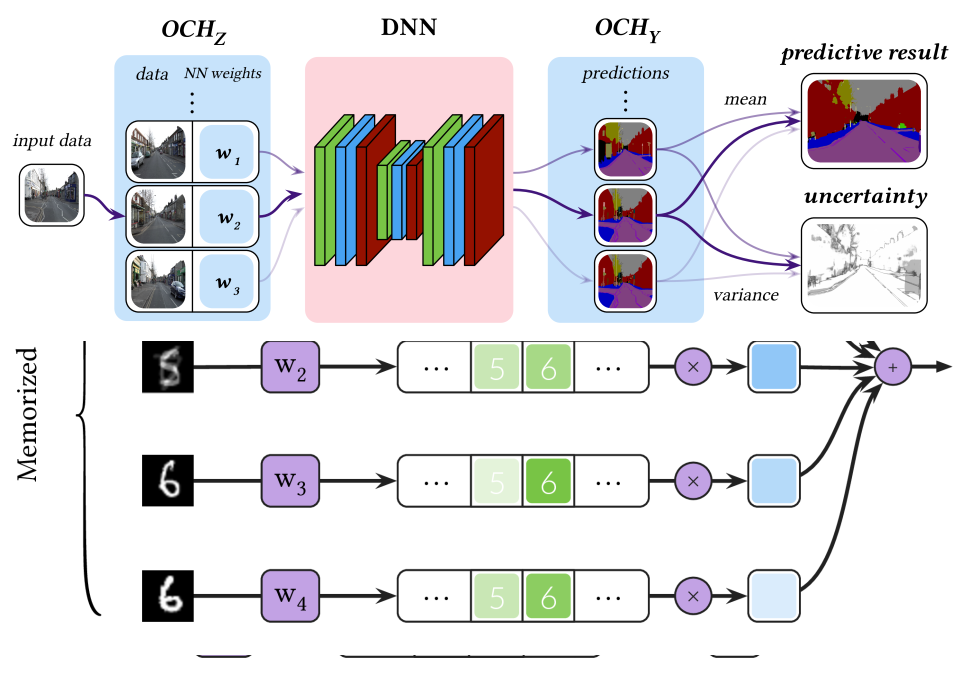

Suppose we have access to memorized input dataset consisting of similar data and corresponding predictions with different weights in the process of inference. Then, the predictive distribution of BNN can be approximated by combining these predictions. Based on this idea, we propose novel predictive distribution called vector quantized BNN (VQ-BNN) inference that approximates BNN inference by using the quantized vectors to speed up calculating the predictive distribution.
In order to reduce the computational burden, VQ-BNN inference performs NN prediction for the observed input only once. Then, it compensates the result with previously memorized predictions. We expect that the predictive distribution of VQ-BNN is analogous to that of BNN, since NN produces similar predictions for similar inputs. For a more sophisticated approximation, the importance of the prediction in the predictive distribution is determined based on the similarity between the observed input and the prediction’s input . To sum up, VQ-BNN inference is as follows:
| (3) |
where and is an importance of with respect to . To estimate this predictive distribution, only needs to be calculated, since remainders are obtained from memorized predictions. This makes the computational performance of VQ-BNN comparable to that of deterministic NN.
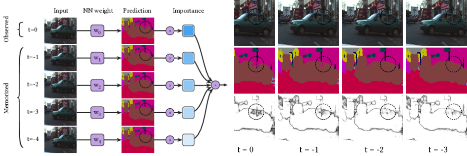
VQ-BNN inference requires memorizing input vectors, similar to the observed input data , and corresponding predictions. To obtain them, we suppose that most of the time-varying data streams are continuously changing. Based thereupon, we prepare the proximate data sequence for VQ-BNN inference on data streams by memorizing the last few data and NN predictions. Also, we propose the importance of a previous data that decreases exponentially over time, i.e., where is hyperparameter and is the time difference between and . In conclusion, VQ-BNN inference for data streams is temporal smoothing with exponentially decaying importance of recent predictions. We summarize VQ-BNN inference in Figure 1.
Results.
We evaluate VQ-BNN with computer vision tasks namely semantic segmentation and depth estimation on a variety of high-dimensional video sequence datasets. The results show that VQ-BNN has almost no degradation in computational performance compared to deterministic NNs. The predictive performance of VQ-BNN is comparable to or superior to that of BNN in various situations.
Contributions.
The main contributions of this work are as follows.
-
•
We propose vector quantized Bayesian neural network (VQ-BNN) inference as an approximation of Bayesian neural network inference to enhance the computational performance.
-
•
We propose temporal smoothing of predictions with exponentially decaying importance by applying VQ-BNN inference to data streams.
-
•
We empirically show that the computational performance of VQ-BNN is almost the same as that of deterministic NN and the predictive performance is comparable to or better than that of BNN on real-world data streams.
2 Vector Quantized
Bayesian Neural Network Inference
Let be a set of data points generated by a source and be an estimated probability distribution of the set of data. The data points are also known as prototypes because they represent the probability. When the source is stationary, the estimated probability represents the observation noise.
We propose a predictive distribution for as an alternative to the predictive distribution of BNN for one data point :
| (4) | ||||
| (5) |
For simplicity, we introduce and in this expression. We call data uncertainty and model uncertainty.
In general, Eq. 5 cannot be solved analytically. We obtain VQ-BNN inference, i.e.,
| (6) |
by approximating . In this equation, we use the following quantized vector samples with importances:
| (7) |
where is a joint of a prototype and a random NN weight sample , i.e., . Then, is a NN prediction for with a random weight. is the importance of with . In Eq. 6, we assume that because is i.i.d.. VQ-BNN inference implies that importances and predictions are required to obtain the predictive distribution. Equation 6 is equivalent to Eq. 3 except that the set of prototypes is denoted by instead of .
Consider the case where the prototypes are given from a noiseless stationary source, i.e., . In this case, all prototypes and importances are the same, and all predictions become . As a result, VQ-BNN inference which is Eq. 6 reduces to BNN inference which is Eq. 2. In the same manner, when consists of data proximate to , the predictive distribution of VQ-BNN is similar to that of BNN.
We can improve the computational performance of calculating predictive distribution by using VQ-BNN inference. Without loss of generality, let be the observed input data. Also, suppose that we have access to memorized prototypes and the corresponding predictions . To calculate the predictive distribution of VQ-BNN, for all prototypes and only for are required since the remainders are obtained from the memorized predictions. Because the time to calculate importances and to aggregate memorized predictions are negligible, it takes almost the same amount of time to perform VQ-BNN inference and to perform NN prediction once.
The case of data stream.
In order to use VQ-BNN as the approximation theory of BNN, we have to take the proximate dataset as prototypes and derive the importances of the prototypes. To calculate the predictive distribution for data streams, VQ-BNN exploits the fact that most real-world data streams change continuously.
Thanks to the temporal proximity of data stream, we take the latest data and the recent subsequence from the data stream as proximate prototypes as follows:
| (8) |
where is integer timestamp and is non-negative number of prototypes from old data streams. In most cases, we need to derive the NN predictions for every data points from the data stream, and it is easy to memorize the sequence of NN predictions .
We define the importance in a similar way as above. Temporal proximity of data stream implies that older data contributes less to the estimated probability distribution for a data stream. Based on this idea, we propose a model in which the importance decreases exponentially over time as follows:
| (9) |
where is given non-negative parameter. is determined experimentally depending on the characteristics of model and data stream. As approaches , the latest prototypes will mainly contribute to the results. As approaches , old prototypes also will equally contribute to the results. In summary, VQ-BNN inference for data stream is temporal smoothing of recent predictions of BNN with exponentially decaying importances.
We have to mention that if the input vector is high-dimensional, VQ-BNN might need a very large number of prototypes to represent the probability of a dataset. The more prototypes are required, the more memory is required, which makes VQ-BNN inference impractical. Despite these concerns, VQ-BNN achieve high prediction performance by using a very small number of prototypes. This is because the relevant data in the data stream are concentrated in a short time interval. Appendix C shows that the semantic segmentation task on a real-world video sequence requires the recent 5 frames to obtain high predictive performance.
There are more complex algorithms that can be used to estimate prototypes from a data stream. For example, (Xu, Shen, and Zhao 2012; Frezza-Buet 2014; Ghesmoune, Lebbah, and Azzag 2016) proposed algorithms that change prototypes depending on data stream. However, these algorithms are not suitable for VQ-BNN since they are too complicated and slow. It is an important drawback because VQ-BNN is developed to achieve high computational performance to process data. The experimental results shows that this simple importance model can achieve high predictive performance.
Implementation.
In order to calculate VQ-BNN inference, we have to determine the prediction parameterized by NN. For classification tasks, we set as a categorical distribution parameterized by the softmax of NN logit:
| (10) |
where is logit of NN, is given by Eq. 8, , and is given by Eq. 9. For regression tasks, are usually modeled to have a Gaussian distribution with the mean of the NN’s result:
| (11) |
where is a given parameter.
For stream processing, we further simplify the VQ-BNN inference with exponentially decaying importance. Let be the predictive distribution for prototypes in . Then, we rewrite as follows:
| (12) | ||||
| (13) |
where . According to this equation, the predictive distribution is the mixture of the latest prediction and the previous predictive distribution.
Training.
The loss function of a BNN, such as evidence lower bound (ELBO) or negative log-likelihood (NLL), depends on a predictive distribution. Therefore, we can calculate the loss function by using VQ-BNN inference instead of by using BNN inference when training NNs.
However, we obtain the posterior distribution in the same way as BNN training for some practical limitations. First, VQ-BNN inference depends on the order of the input data stream. It increases the implementation complexity of training with VQ-BNN inference. Next, many training datasets do not have all the labels corresponding to the input data stream. To derive the predictive distribution for an input with a label, VQ-BNNs have to predict the result for the previous inputs without a label. It significantly increases the time required for the NN training process. Experiments show that VQ-BNN inference achieves high predictive performance even though it uses the posterior distribution by BNN training.
3 Experiments
| Method | Bat Thr (Img/Sec) | Str Thr (Img/Sec) | NLL | Acc (%) | Acc90 (%) | Unc90 (%) | IoU (%) | IoU90 (%) | Freq90 (%) | ECE (%) |
|---|---|---|---|---|---|---|---|---|---|---|
| DNN | 27.5 | 10.5 | 0.314 | 91.1 | 96.1 | 61.3 | 66.1 | 77.7 | 86.4 | 4.31 |
| BNN | 0.824 | 0.788 | 0.276 | 91.8 | 96.5 | 63.0 | 68.1 | 79.9 | 86.8 | 3.71 |
| VQ-BNN | 25.5 | 9.41 | 0.253 | 92.0 | 97.4 | 72.4 | 68.6 | 83.7 | 83.1 | 2.24 |
This section evaluates the performance of VQ-BNN in three sets of experiments. The first experiment visualizes the characteristics of VQ-BNN with simple linear regression on synthetic data. The second experiment performs semantic segmentation on high-dimensional real-world video sequences. This classification task compares the performances of VQ-BNN with other baselines of deep NNs in a practical situation. The last experiment performs monocular depth estimation on high-dimensional real-world video sequences. This experiment compares the performance of VQ-BNN in a regression task.
Baselines.
We compare the following three methods in the experiments:
-
•
DNN. Let be predictive probability of deterministic NN (DNN) where is NN logits for classification tasks. It is easy to implement, but it deviates from the true classification probability when the NN is deepened, broadened, and regularized well (Guo et al. 2017).
-
•
BNN. BNNs use the MC estimator Eq. 2 to calculate a predictive distribution. It is difficult to analytically determine the sufficient number of NN weight samples to converge predictive distribution. Instead, we experimentally set the number of the samples to 30—i.e., BNNs with MC dropout (Gal and Ghahramani 2016) layers predict results with 30 forward passes in Section 3.2 and Section 3.3—so that the negative log-likelihood (NLL) converge. Appendix B shows the predictive performance of BNN for different numbers of forward passes.
-
•
VQ-BNN. As explained in Section 2, VQ-BNN inference uses the same model and weight distribution as BNN. In all experiments, we use the same hyperparameters, and , which implies that VQ-BNN is not overly sensitive to hyperparameter selection. See Appendix C for performance changes according to hyperparameters.
3.1 Simple Linear Regression
This experiment uses a linear regression model to find out the characteristics of VQ-BNN. The posteriors for BNN and VQ-BNN are given by and . The weights for DNN are expected values of the posteriors, i.e., and . The distribution of time-varying input data streams is given by where is integer timestamp from and .
Results.
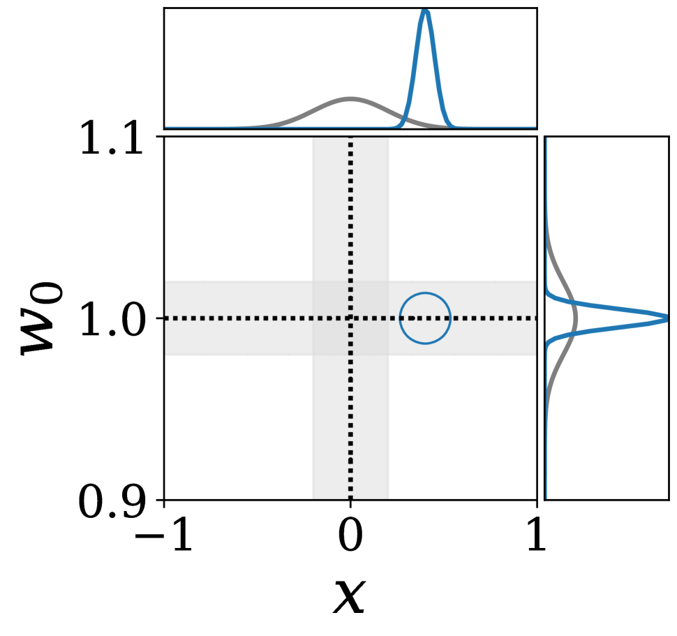
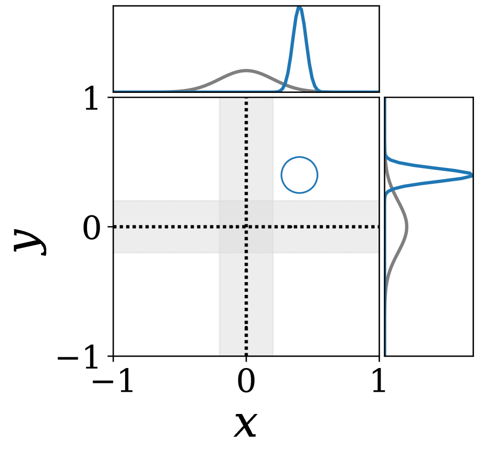
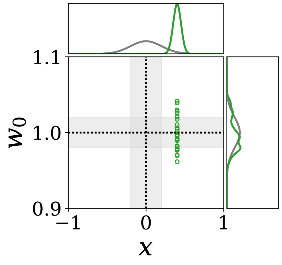
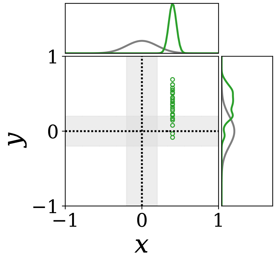
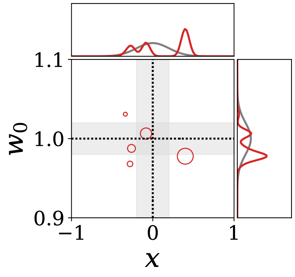
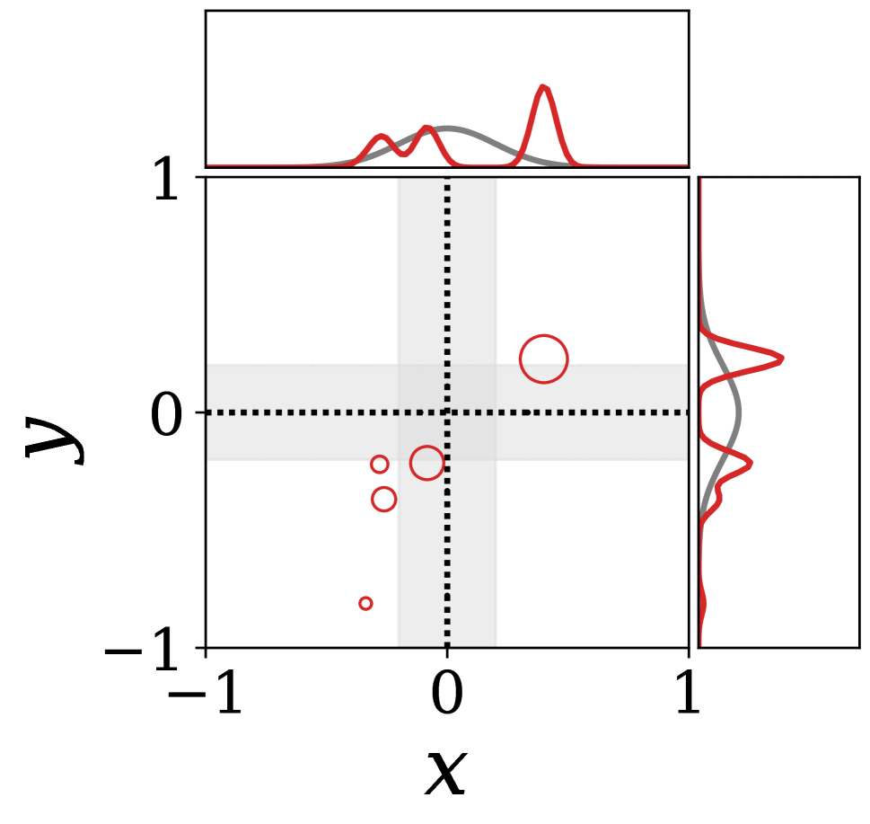
Figure 2 shows the probability distributions approximated by prototypes at . In this figure, the upper row displays approximated distributions of input and NN weight prototypes, i.e., , and the lower row shows approximated distributions of output prototypes with data, i.e., . The sizes of the circle indicate the importances of each prototype. It also show the three kinds of marginal distributions: the probability distribution of data , the posterior distribution of NN weight , and the predictive distribution . is omitted from in these figures, but it behaves like .
To make a prediction, DNN uses a data point and a point-estimated NN weight. BNN uses a data point and a NN weight distribution, instead of point-estimated weight. VQ-BNN estimates predictive distribution by using the NN weight distribution and the set of data from the past to now that represents the probability distribution of data. In other words, VQ-BNN without distribution of is equivalent to BNN, and BNN without distribution of is equivalent to DNN.
In this experiment, the most recent data sample is . It is a noisy value because the expected value of at is . Since DNN and BNN only use the most recent data point to predict results, their predictive distributions are highly dependent on the noise of the data. As a result, an unexpected data makes the predictive distributions of DNN and BNN inaccurate. In contrast, VQ-BNN smoothen the predictive distribution by using predictions with respect to past data. Therefore, the predictive distributions of VQ-BNN are robust to the noise of data and its prediction.
Implications.
These results imply that VQ-BNN may give a more accurate predictive result than BNN when the input and its prediction are noisy. Also, VQ-BNN is less likely to be overconfident than BNN since VQ-BNN uses both NN weight distribution and a probability distribution of data. For this reason, VQ-BNN might be better calibrated than BNN.
3.2 Semantic Segmentation
Semantic segmentation experiment, which is a pixel-wise classification, evaluates the computational and predictive performance of VQ-BNN with a modern deep NN in practical situation. We use the CamVid dataset (Brostow, Fauqueur, and Cipolla 2009) consisting of 360480 pixels 30 frame-per-second (fps) video sequences of real-world day and dusk road scenes. We use U-Net (Ronneberger, Fischer, and Brox 2015) as the backbone architecture. Bayesian U-Net, similar to (Kendall, Badrinarayanan, and Cipolla 2015), contains six MC dropout layers. For more information about experimental settings, see Section A.1. See Section D.1 for experiments on a different dataset and model.
Computational performance.
The throughput (Bat Thr, 111We use arrows to indicate which direction is better.) column of Table 1 shows the number of video frames processed by each model per second in batch processing. In this table, VQ-BNN processes 25.5 images per second, which is only 7% slower than DNN, and 33 faster than BNN. Likewise, the throughput column for stream processing (Str Thr, ) shows that VQ-BNN processes 9.41 images per second in stream processing, which is only 10% slower than DNN, and 12 faster than BNN.
In conclusion, the computational performance of VQ-BNN is comparable to that of DNN and significantly better than that of BNN. See Section D.1 for more information.
Predictive performance.
We use global pixel accuracy (Acc, ) and mean Intersection over Union (IoU, ) to evaluate predictive results. We also use NLL (), Expected Calibration Error (ECE, ) (Naeini, Cooper, and Hauskrecht 2015; Guo et al. 2017), and the following metrics to measure predictive uncertainty:
-
•
Accuracy-90 (Acc90, ). If NN is confident in its prediction, it must be accurate. Therefore, we select predictions with confidence higher than 90% and measure the accuracy, i.e., . Likewise, we measure IoU for the confident predictions (IoU90, ).
-
•
Unconfidence-90 (Unc90, ). If the prediction of NN is incorrect, NN should not be confident in it. Therefore, we measure the probability of prediction which is not confident for incorrect prediction, i.e., .
-
•
Frequency-90 (Freq90, ). Even if NN derives reliable uncertainty, the model is ineffectual if it rarely predicts high-confidence results. Therefore, we measure the percentage of predictions with confidence, i.e., .
The NLL to ECE columns of the Table 1 show the quantitative comparison of the predictive performance for each method. This table shows that the predictive performance of BNN is better than that of DNN. Also, according to uncertainty metrics, VQ-BNN predict uncertainty better than BNN. Moreover, Acc and IoU show that VQ-BNN predicts more accurate results than BNN, which is beyond our expectations.
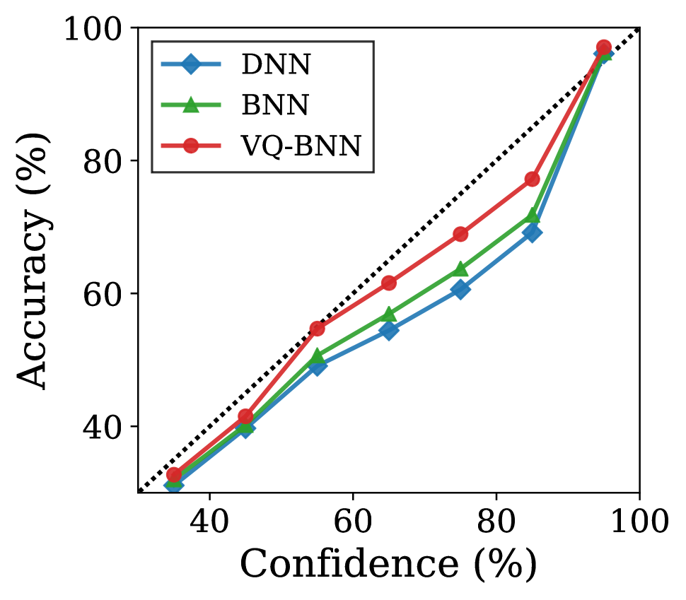
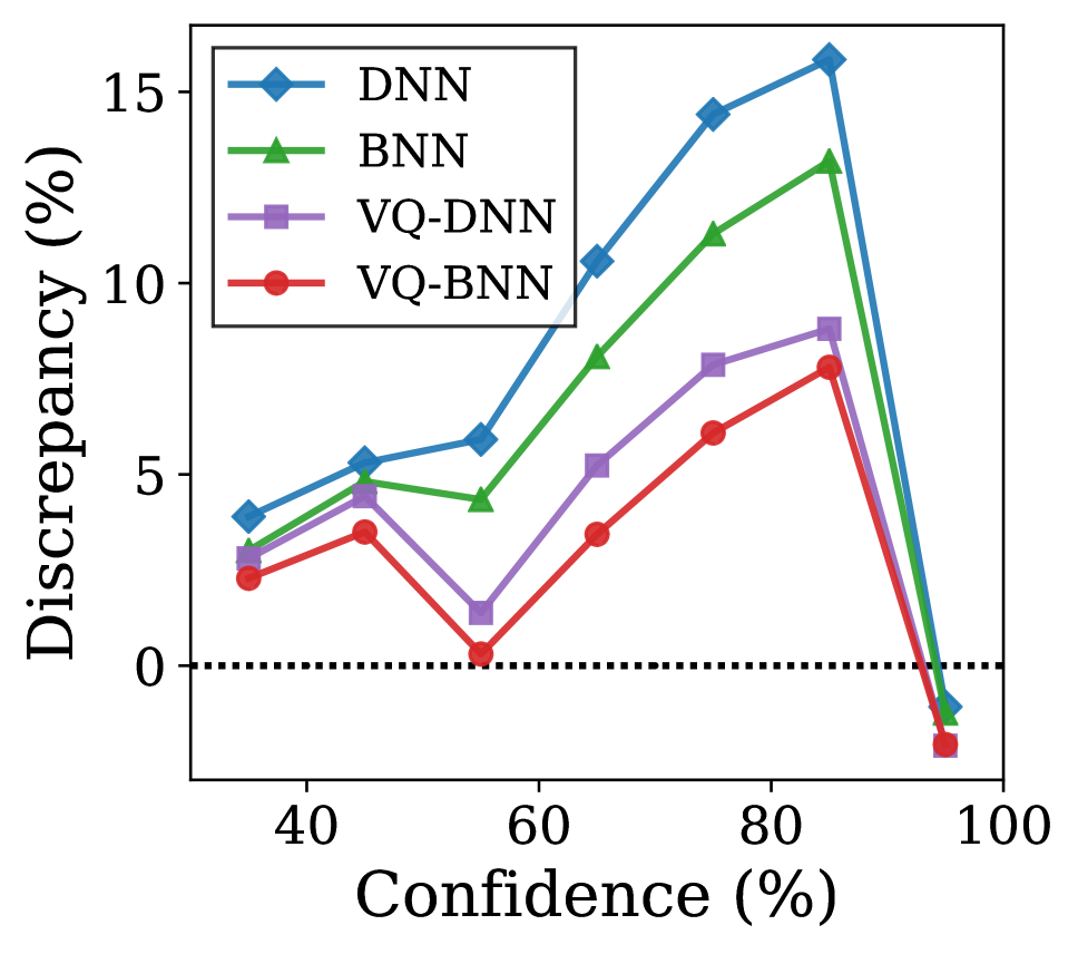
Figure 3 shows the reliability diagram (Niculescu-Mizil and Caruana 2005; Naeini, Cooper, and Hauskrecht 2015; Guo et al. 2017). As shown in this figure, DNN is miscalibrated; there is significant discrepancy between confidence and accuracy. In contrast, VQ-BNN is better calibrated than DNN, and surprisingly better than BNN.
According to these results, VQ-BNN is the most appropriate method not only to distinguish uncertain predictions but also to predict accurate results. Table 5 in Section D.1 shows the predictive performance of VQ-BNN in various situations. Section D.1 also evaluates VQ-DNN, which is the temporal smoothing of DNN’s predictions. Its predictive performance is better than that of DNN, but worse than that of VQ-BNN.
Analysis.
The results of Section 3.1 imply that VQ-BNN is effective in compensating for noisy predictions. For semantic segmentation task, the data that derives inaccurate results mainly correspond to the edges of objects.
VQ-BNN smoothens the predictive distribution by using past predictions. Because objects move slowly every frame, the uncertainty predicted by VQ-BNN is located at the edges of the objects. Even if VQ-BNN accidentally predicts a wrong result for the most recent frame, the past predictions compensate for this error. Figure 4 shows that predictive uncertainty of VQ-BNN is mainly located at the edge of the car, and past predictions correct the most recent incorrect predictions for the car.
We quantitatively show that VQ-BNN achieves higher predictive performance than other methods at the edges of objects. We measure predictive performance for pixels representing the object edges, and we call it edge predictive performance. The results of this experiment show that the edge predictive performance lags behind the predictive performance for all pixels. It implies that there are many inaccurate predictions on object edges. In addition, the difference in the edge predictive performance between VQ-BNN and BNN is greater than the difference in the predictive performance between VQ-BNN and BNN. This implies that VQ-BNN works well for edge pixels. See Section D.1 and Table 6 for more details on the edge predictive performance.
VQ-BNN relies on temporal consistency of data streams. Section D.1 evaluate the sensitivity to the temporal consistency, and the result show that the predictive performance is degraded when temporal consistency decreases.
3.3 Depth Estimation
| Method | Bat Thr (Img/Sec) | Str Thr (Img/Sec) | NLL | RMSE (m) |
|---|---|---|---|---|
| DNN | 54.0 | 14.5 | 1.55 | 0.804 |
| BNN | 1.59 | 1.61 | 1.10 | 0.705 |
| VQ-BNN | 50.8 | 13.6 | 1.09 | 0.700 |
Monocular depth estimation experiment shows the performance of VQ-BNN with a deep NN in a regression task on a real-world dataset. We use the NYUDv2 dataset (Nathan Silberman and Fergus 2012), which consists of 240320 pixels 20-30 fps video sequences from a variety of indoor scenes. As in Section 3.2, we use U-Net and Bayesian U-Net as backbone architectures. For more information about experimental settings, see Section A.2.
Computational performance.
The throughput for batch processing (Bat Thr, ) of Table 2 shows the number of video frames processed by each model per second. In this table, VQ-BNN processes 54.0 images per second, which is only 6% slower than DNN, and 32 faster than BNN. Similarly, the throughput for stream processing (Str Thr, ) shows that VQ-BNN processes 13.6 images per second in stream processing, which is only 6% slower than that of DNN, and 8 faster than that of BNN. These results are consistent with the results in Section 3.2; the computational performance of VQ-BNN is significantly better than that of BNN, and is similar to that of DNN. See Section D.2 for more information.
Predictive performance.
We use root-mean-square error (RMSE, ) to evaluate predictive results for depth estimation. We use NLL to evaluate predictive uncertainty.
RMSE and NLL columns of Table 2 show predictive performances for each method. This table shows that both RMSE and NLL of VQ-BNN are the lowest among those of the three methods. In conclusion, VQ-BNN is the most appropriate method for predicting accurate predictive results as well as reliable uncertainty in the regression task. See Section D.2 for more information on depth regression experiment.
4 Related Work
Several sampling-free BNNs, e.g. (Hernández-Lobato and Adams 2015; Wang, Xingjian, and Yeung 2016; Wu et al. 2018), were proposed recently and they might be a solution to the problem that BNNs require multiple NN predictions. Sampling-free BNNs approximate the posterior and the probability of layer’s outputs using a simple type of parametric distribution such as Gaussian distribution or exponential family. Therefore, they predict results with one or two forward passes.
However, neural networks used in real world situations have dozens or more of layers, and sampling-free BNNs are not suitable for deep NNs. To the best of our knowledge, most sampling-free BNN have been evaluated only with a couple of layers on low-dimensional data such as UCI datasets. One of the reasons is that the Gaussian approximation in sampling-free BNNs can be inaccurate to represent real-world probabilities. Since the discrepancy between true values and approximate values accumulates in every NN layer, the error of deep sampling-free BNNs becomes not negligible. Moreover, in many cases, sampling-free BNN can not use variational inference to obtain a posterior because ELBO is not amenable. For these reasons, we mainly consider sampling-based BNNs for comparison in this paper. Recently, (Gast and Roth 2018) and (Haußmann, Hamprecht, and Kandemir 2020) applied sampling-free BNNs to LeNet. (Postels et al. 2019) applied it to SegNet; however, the neural network does not predict well-calibrated results. See Appendix E for more details on the sampling-free BNN.
(Riquelme, Tucker, and Snoek 2018) and (Kohl et al. 2018), which utilize Bayesian methods only in the last layer, predict results efficiently. However, this approach generally achieves poor predictive performance and are not robust to corrupted inputs (Ovadia et al. 2019).
A temporal smoothing has been widely used to reduce noise for accurate time-series forecasting (Pai and Lin 2005; Ediger and Akar 2007; Benvenuto et al. 2020). (Zhang 2003; Khashei and Bijari 2010; Chan et al. 2011) combined it with NN to improve accuracy for forecasting tasks on low-dimensional data streams. In this paper, we show that the temporal smoothing can significantly improve the computational performance of BNNs on high-dimensional data streams.
5 Conclusion
We present VQ-BNN inference, which is a novel approximation of BNN inference, to improve the computational performance of BNN inference for data streams. BNN inference iteratively executes NN prediction for a data, which makes it dozens of times slower. In contrast, VQ-BNN inference executes NN prediction only once for the latest data from the data stream, and compensate the result with previously memorized predictions. Specifically, VQ-BNN inference for data streams is temporal smoothing of recent predictions with exponentially decaying importance, and it is easy to implement. This method results in an order of magnitude times improvement in computational performance compared to BNN. Experiments with computer vision tasks such as semantic segmentation on various real-world datasets show that the computational performance of VQ-BNN is almost the same as that of deterministic NN, and the predictive performance is comparable to or even superior to that of BNN. Since the computational performance of deterministic NN is the best we can expect, VQ-BNN is an efficient method to estimate uncertainty.
Acknowledgement
This work was supported by Samsung Research Funding Center of Samsung Electronics under Project Number SRFC-IT1801-10.
References
- Abadi et al. (2016) Abadi, M.; Agarwal, A.; Barham, P.; Brevdo, E.; Chen, Z.; Citro, C.; Corrado, G. S.; Davis, A.; Dean, J.; Devin, M.; et al. 2016. Tensorflow: Large-scale machine learning on heterogeneous distributed systems. arXiv preprint arXiv:1603.04467 .
- Badrinarayanan, Kendall, and Cipolla (2017) Badrinarayanan, V.; Kendall, A.; and Cipolla, R. 2017. Segnet: A deep convolutional encoder-decoder architecture for image segmentation. IEEE transactions on pattern analysis and machine intelligence 39(12): 2481–2495.
- Benvenuto et al. (2020) Benvenuto, D.; Giovanetti, M.; Vassallo, L.; Angeletti, S.; and Ciccozzi, M. 2020. Application of the ARIMA model on the COVID-2019 epidemic dataset. Data in brief 105340.
- Brostow, Fauqueur, and Cipolla (2009) Brostow, G. J.; Fauqueur, J.; and Cipolla, R. 2009. Semantic object classes in video: A high-definition ground truth database. Pattern Recognition Letters 30(2): 88–97.
- Chan et al. (2011) Chan, K. Y.; Dillon, T. S.; Singh, J.; and Chang, E. 2011. Neural-network-based models for short-term traffic flow forecasting using a hybrid exponential smoothing and Levenberg–Marquardt algorithm. IEEE Transactions on Intelligent Transportation Systems 13(2): 644–654.
- Cordts et al. (2016) Cordts, M.; Omran, M.; Ramos, S.; Rehfeld, T.; Enzweiler, M.; Benenson, R.; Franke, U.; Roth, S.; and Schiele, B. 2016. The cityscapes dataset for semantic urban scene understanding. In Proceedings of the IEEE conference on computer vision and pattern recognition, 3213–3223.
- Ediger and Akar (2007) Ediger, V. Ş.; and Akar, S. 2007. ARIMA forecasting of primary energy demand by fuel in Turkey. Energy policy 35(3): 1701–1708.
- Finn, Xu, and Levine (2018) Finn, C.; Xu, K.; and Levine, S. 2018. Probabilistic model-agnostic meta-learning. In Advances in Neural Information Processing Systems, 9516–9527.
- Fortunato, Blundell, and Vinyals (2017) Fortunato, M.; Blundell, C.; and Vinyals, O. 2017. Bayesian recurrent neural networks. arXiv preprint arXiv:1704.02798 .
- Frezza-Buet (2014) Frezza-Buet, H. 2014. Online computing of non-stationary distributions velocity fields by an accuracy controlled growing neural gas. Neural Networks 60: 203–221.
- Gal and Ghahramani (2016) Gal, Y.; and Ghahramani, Z. 2016. Dropout as a Bayesian Approximation - Representing Model Uncertainty in Deep Learning. ICML .
- Gast and Roth (2018) Gast, J.; and Roth, S. 2018. Lightweight probabilistic deep networks. In Proceedings of the IEEE Conference on Computer Vision and Pattern Recognition, 3369–3378.
- Ghesmoune, Lebbah, and Azzag (2016) Ghesmoune, M.; Lebbah, M.; and Azzag, H. 2016. A new growing neural gas for clustering data streams. Neural Networks 78: 36–50.
- Guo et al. (2017) Guo, C.; Pleiss, G.; Sun, Y.; and Weinberger, K. Q. 2017. On calibration of modern neural networks. In Proceedings of the 34th International Conference on Machine Learning-Volume 70, 1321–1330. JMLR. org.
- Haußmann, Hamprecht, and Kandemir (2020) Haußmann, M.; Hamprecht, F. A.; and Kandemir, M. 2020. Sampling-free variational inference of bayesian neural networks by variance backpropagation. In Uncertainty in Artificial Intelligence, 563–573. PMLR.
- Hernández-Lobato and Adams (2015) Hernández-Lobato, J. M.; and Adams, R. P. 2015. Probabilistic Backpropagation for Scalable Learning of Bayesian Neural Networks. NIPS stat.ML.
- Kahn et al. (2017) Kahn, G.; Villaflor, A.; Pong, V.; Abbeel, P.; and Levine, S. 2017. Uncertainty-aware reinforcement learning for collision avoidance. arXiv preprint arXiv:1702.01182 .
- Kendall, Badrinarayanan, and Cipolla (2015) Kendall, A.; Badrinarayanan, V.; and Cipolla, R. 2015. Bayesian segnet: Model uncertainty in deep convolutional encoder-decoder architectures for scene understanding. arXiv preprint arXiv:1511.02680 .
- Kendall and Gal (2017) Kendall, A.; and Gal, Y. 2017. What uncertainties do we need in bayesian deep learning for computer vision? In Advances in neural information processing systems, 5574–5584.
- Kendall, Gal, and Cipolla (2018) Kendall, A.; Gal, Y.; and Cipolla, R. 2018. Multi-task learning using uncertainty to weigh losses for scene geometry and semantics. In Proceedings of the IEEE Conference on Computer Vision and Pattern Recognition, 7482–7491.
- Khashei and Bijari (2010) Khashei, M.; and Bijari, M. 2010. An artificial neural network (p, d, q) model for timeseries forecasting. Expert Systems with applications 37(1): 479–489.
- Kohl et al. (2018) Kohl, S.; Romera-Paredes, B.; Meyer, C.; De Fauw, J.; Ledsam, J. R.; Maier-Hein, K.; Eslami, S.; Jimenez Rezende, D.; and Ronneberger, O. 2018. A probabilistic u-net for segmentation of ambiguous images. Advances in neural information processing systems 31: 6965–6975.
- Naeini, Cooper, and Hauskrecht (2015) Naeini, M. P.; Cooper, G.; and Hauskrecht, M. 2015. Obtaining well calibrated probabilities using bayesian binning. In Twenty-Ninth AAAI Conference on Artificial Intelligence.
- Nathan Silberman and Fergus (2012) Nathan Silberman, Derek Hoiem, P. K.; and Fergus, R. 2012. Indoor Segmentation and Support Inference from RGBD Images. In ECCV.
- Niculescu-Mizil and Caruana (2005) Niculescu-Mizil, A.; and Caruana, R. 2005. Predicting good probabilities with supervised learning. In Proceedings of the 22nd international conference on Machine learning, 625–632. ACM.
- Osband, Aslanides, and Cassirer (2018) Osband, I.; Aslanides, J.; and Cassirer, A. 2018. Randomized prior functions for deep reinforcement learning. In Advances in Neural Information Processing Systems, 8617–8629.
- Ovadia et al. (2019) Ovadia, Y.; Fertig, E.; Ren, J.; Nado, Z.; Sculley, D.; Nowozin, S.; Dillon, J.; Lakshminarayanan, B.; and Snoek, J. 2019. Can you trust your model’s uncertainty? Evaluating predictive uncertainty under dataset shift. In Advances in Neural Information Processing Systems, 13991–14002.
- Pai and Lin (2005) Pai, P.-F.; and Lin, C.-S. 2005. A hybrid ARIMA and support vector machines model in stock price forecasting. Omega 33(6): 497–505.
- Postels et al. (2019) Postels, J.; Ferroni, F.; Coskun, H.; Navab, N.; and Tombari, F. 2019. Sampling-free Epistemic Uncertainty Estimation Using Approximated Variance Propagation. In Proceedings of the IEEE International Conference on Computer Vision, 2931–2940.
- Riquelme, Tucker, and Snoek (2018) Riquelme, C.; Tucker, G.; and Snoek, J. 2018. Deep bayesian bandits showdown: An empirical comparison of bayesian deep networks for thompson sampling. arXiv preprint arXiv:1802.09127 .
- Ronneberger, Fischer, and Brox (2015) Ronneberger, O.; Fischer, P.; and Brox, T. 2015. U-net: Convolutional networks for biomedical image segmentation. In International Conference on Medical image computing and computer-assisted intervention, 234–241. Springer.
- Simonyan and Zisserman (2014) Simonyan, K.; and Zisserman, A. 2014. Very deep convolutional networks for large-scale image recognition. arXiv preprint arXiv:1409.1556 .
- Wang, Xingjian, and Yeung (2016) Wang, H.; Xingjian, S.; and Yeung, D.-Y. 2016. Natural-parameter networks: A class of probabilistic neural networks. In Advances in Neural Information Processing Systems, 118–126.
- Wu et al. (2018) Wu, A.; Nowozin, S.; Meeds, E.; Turner, R. E.; Hernandez-Lobato, J. M.; and Gaunt, A. L. 2018. Deterministic variational inference for robust bayesian neural networks. arXiv preprint arXiv:1810.03958 .
- Xu, Shen, and Zhao (2012) Xu, Y.; Shen, F.; and Zhao, J. 2012. An incremental learning vector quantization algorithm for pattern classification. Neural Computing and Applications 21(6): 1205–1215.
- Yoon et al. (2018) Yoon, J.; Kim, T.; Dia, O.; Kim, S.; Bengio, Y.; and Ahn, S. 2018. Bayesian model-agnostic meta-learning. In Advances in Neural Information Processing Systems, 7332–7342.
- Zhang (2003) Zhang, G. P. 2003. Time series forecasting using a hybrid ARIMA and neural network model. Neurocomputing 50: 159–175.
Appendix A Experimental Setup and Datasets
| Dataset | |||
| CamVid | 3604803 | 36048011 | 421 |
| CityScape | 51210243 | 512102419 | 2975 |
| NYUDv2 | 2403203 | 2403201 | 47584 |
We conduct all the experiments with the Intel Xeon W-2123 Processor, 32GB memory, and a single GeForce RTX 2080 Ti. NN models are implemented in TensorFlow (Abadi et al. 2016).
A.1 Semantic Segmentation
Section 3.2, Section D.1, and Appendix E conduct semantic segmentation experiments. In these experiments, we use two different kinds of neural network architectures: U-Net (Ronneberger, Fischer, and Brox 2015) based on VGG-16 (Simonyan and Zisserman 2014) and SegNet (Badrinarayanan, Kendall, and Cipolla 2017). We also use Bayesian U-Net and Bayesian SegNet (Kendall, Badrinarayanan, and Cipolla 2015) as baselines. Bayesian U-Net, similar to (Kendall, Badrinarayanan, and Cipolla 2015), contains six MC dropout (Gal and Ghahramani 2016) layers behind the layers that receive the smallest feature map sizes.
We use the CamVid dataset (Brostow, Fauqueur, and Cipolla 2009) and the CityScape dataset (Cordts et al. 2016) in the semantic segmentation experiments. For the CamVid dataset, we resize images to 360480 pixels bilinearly from 720960 pixels. For the CityScape dataset, we resize images to 5121024 pixels from 10242048 pixels. For the CityScape dataset, we use validation set as test set because only the video sequence corresponding to the validation set has been disclosed. We use reduced label lists on both datasets. Table 3 summarizes the information of datasets.
NNs are trained using categorical cross-entropy loss, with Adam optimizer with a constant learning rate of 0.001, , and . Batch size is limited to 3 because of memory limitation. We consider basic data augmentation techniques: random cropping and horizontal flipping. Since the datasets are imbalanced, we consider median frequency balancing. For the CamVid dataset and the CityScape dataset, we train NNs for 100 epochs and 500 epochs, respectively.
We set as a categorical distribution parameterized by the softmax of NN logit, then the predictive distribution of BNN is where is number of NN weight samples and is logit of NN. The predictive distribution of VQ-BNN is Eq. 10. The reported metrics are the mean values and standard deviations of five evaluations. For the CityScape, the metrics are the mean and standard deviations from the final five epochs. To optimize the predictive performances, we set hyperparameters of VQ-BNN and to and , respectively. We report how NLL changes across various hyperparameters in Appendix C.
A.2 Depth Estimation
Section 3.3 and Section D.2 conduct monocular depth estimation experiments. In these experiment, we use the same U-Net, SegNet, Bayesian U-Net, and Bayesian SegNet as above.
We use NYU Depth Dataset V2 (NYUDv2) (Nathan Silberman and Fergus 2012) that resizes 480640 pixels to 240320 pixels in the experiments. NYUDv2 contains 464 scenes, and 249 scenes are used for training. We use the remaining 215 scenes for evaluation.
NNs are optimized with mean squared error loss function and Adam optimizer with a constant learning rate of 0.001, , and . Batch size is limited to 3. We consider simple data augmentation techniques: random cropping and horizontal flipping. We train NN for 6 epochs.
Since depth estimation is a pixel-wise regression task, we set as a normal distribution where is hyperparameter. Then, the predictive distribution of BNN is . The predictive distribution of VQ-BNN is given by Eq. 11 in theory, but this expression is a bit tricky to implement. Instead, we rewrite the distribution as where and . Then, we use normal distribution to approximate the distribution of as follows:
| (14) | ||||
| (15) |
where and are weighted mean and weighted variance of , i.e.,
| (16) | ||||
| (17) |
The reported metrics are the mean and standard deviations from , , and epochs. We set to , which is the value that minimizes NLL on validation set. We set hyperparameters of VQ-BNN and to and , respectively, as above.
Appendix B Predictive Performance of BNN for Different Numbers of Forward Passes
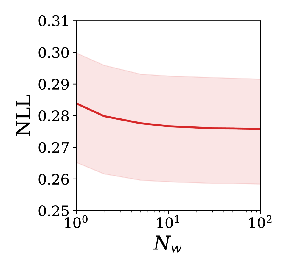
BNNs in experiments contain MC dropout layers and require multiple forward passes to predict result. Figure 5 shows the predictive performance represented by NLL of the Bayesian U-Net for the number of forward passes on the CamVid dataset.
This figure shows that the predictive performance of BNN improves up to 30 forward passes. However, there is little difference between the predictive performance for 30 forward passes and 50 forward passes. According to this result, BNN requires at least 30 forward passes to get the best predictive performance, so we execute 30 predictive inference in all experiments.
Appendix C Effects of Hyperparameters
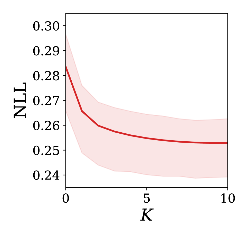
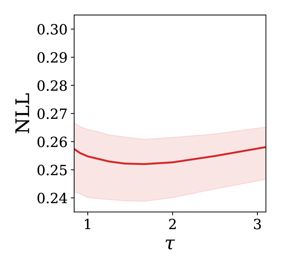
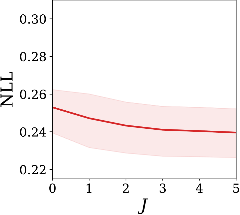
VQ-BNN has two independent hyperparameters: and . Figure 6 shows how NLL changes over the variuos hyperparameters in the semantic segmentation experiment on the CamVid dataset. As shown in this figure, as increases, NLL decreases, and the NLL stagnates when goes over 5. The higher the , the lower the NLL, until 1.25.
With high and , VQ-BNN uses more previous predictions to derive the predictive distribution. In this case, past predictions compensate for the most recent prediction as shown in this paper. As a result, with high and , VQ-BNN exhibits lower NLL. However, when gets higher than a certain point ( in this figure), the data uncertainty is too high to estimate results. NLL is minimized when model uncertainty and data uncertainty are balanced.
Appendix D Extended Informations of Experiments
Section 3 makes a computer vision experiments namely semantic segmentation and depth estimation to show the performance of VQ-BNN. This section shows additional information on these experiments.
We use the additional method in the experiments:
-
•
VQ-DNN. VQ-DNN is temporal exponential smoothing of DNN’s predictions. In other words, it is almost the same as VQ-BNN inference, but it uses deterministic NN weight obtained from DNN, instead of probabilistic NN weights. This method shows the effect of data uncertainty, when it is applied to the DNN. This technique is particularly useful when BNN is not accessible. The experimental results show that VQ-DNN achieves better predictive performance than vanilla DNNs in computer vision tasks.
D.1 Semantic Segmentation
| Dataset & Model | Method | Bat Thr (Img/Sec) | Str Thr (Img/Sec) | NLL | Acc (%) | Acc90 (%) | Unc90 (%) | IoU (%) | IoU90 (%) | Freq90 (%) | ECE (%) |
|---|---|---|---|---|---|---|---|---|---|---|---|
| CamVid & U-Net | DNN | 27.51.2 | 10.51.7 | 0.3140.021 | 91.11.3 | 96.10.3 | 61.36.4 | 66.12.7 | 77.70.6 | 86.43.5 | 4.310.37 |
| BNN | 0.8240.003 | 0.7880.033 | 0.2760.012 | 91.80.3 | 96.50.2 | 63.03.0 | 68.10.7 | 79.90.5 | 86.81.2 | 3.710.23 | |
| VQ-DNN | 27.01.6 | 10.31.3 | 0.2840.023 | 91.21.2 | 97.00.2 | 71.05.2 | 66.62.7 | 81.70.6 | 83.03.5 | 3.000.33 | |
| VQ-BNN | 25.51.1 | 9.410.84 | 0.2530.009 | 92.00.2 | 97.40.2 | 72.52.8 | 68.60.8 | 83.70.8 | 83.11.3 | 2.240.30 | |
| CamVid & SegNet | DNN | 37.01.5 | 11.91.6 | 0.6050.090 | 86.20.7 | 92.61.2 | 55.16.4 | 51.61.3 | 60.93.1 | 83.72.3 | 8.381.17 |
| BNN | 1.130.01 | 1.120.03 | 0.4260.026 | 86.80.8 | 96.10.5 | 78.52.1 | 53.71.1 | 71.21.8 | 73.61.5 | 4.020.75 | |
| VQ-DNN | 35.82.6 | 11.41.3 | 0.4830.099 | 86.70.8 | 94.61.3 | 68.36.6 | 52.31.4 | 65.34.1 | 78.82.5 | 6.141.38 | |
| VQ-BNN | 34.82.0 | 11.31.2 | 0.4330.027 | 86.20.9 | 96.50.9 | 81.85.6 | 52.71.2 | 72.42.2 | 70.65.9 | 3.551.71 | |
| CityScape & U-Net | DNN | 9.200.22 | 7.440.80 | 0.3250.057 | 91.41.6 | 96.20.4 | 60.94.9 | 60.05.9 | 71.74.1 | 87.53.9 | 4.300.29 |
| BNN | 0.2850.003 | 0.2850.003 | 0.2780.051 | 92.41.3 | 97.30.3 | 68.54.0 | 60.73.9 | 75.31.7 | 86.83.8 | 2.950.23 | |
| VQ-DNN | 9.090.34 | 7.390.68 | 0.2960.050 | 91.71.5 | 97.50.4 | 75.55.2 | 60.65.7 | 75.53.9 | 78.75.8 | 2.000.56 | |
| VQ-BNN | 8.590.25 | 6.530.50 | 0.2820.048 | 92.21.5 | 97.90.2 | 78.13.1 | 60.43.9 | 76.51.5 | 80.03.9 | 1.530.23 | |
| CityScape & SegNet | DNN | 12.40.7 | 8.890.55 | 0.3610.011 | 89.60.4 | 96.00.2 | 67.61.0 | 54.40.6 | 69.30.5 | 83.90.5 | 4.800.29 |
| BNN | 0.3930.006 | 0.3930.005 | 0.3280.004 | 89.40.2 | 97.80.1 | 84.40.3 | 53.30.3 | 77.60.4 | 75.80.3 | 1.790.10 | |
| VQ-DNN | 12.30.8 | 8.770.49 | 0.3270.008 | 90.40.3 | 97.60.1 | 80.80.6 | 55.00.5 | 73.50.3 | 77.30.7 | 1.880.11 | |
| VQ-BNN | 11.70.6 | 8.050.677 | 0.3440.004 | 89.10.2 | 98.10.1 | 87.70.2 | 52.40.2 | 77.30.6 | 71.30.3 | 0.7840.040 |
| Dataset & Model | Method | Bat Thr (Img/Sec) | Str Thr (Img/Sec) | NLL | RMSE (m) | Rel | |||
|---|---|---|---|---|---|---|---|---|---|
| NYUDv2 & U-Net | DNN | 54.02.6 | 14.52.1 | 1.550.36 | 0.8040.073 | 0.2980.034 | 0.5600.029 | 0.8380.011 | 0.9390.010 |
| BNN | 1.590.02 | 1.610.03 | 1.100.03 | 0.7040.018 | 0.2930.012 | 0.5730.023 | 0.8340.016 | 0.9410.005 | |
| VQ-DNN | 52.82.8 | 13.91.5 | 1.140.07 | 0.7500.081 | 0.2990.037 | 0.5650.034 | 0.8380.016 | 0.9400.012 | |
| VQ-BNN | 50.83.1 | 13.61.4 | 1.090.03 | 0.7000.016 | 0.2890.007 | 0.5810.014 | 0.8390.010 | 0.9420.003 | |
| NYUDv2 & SegNet | DNN | 68.80.3 | 15.00.3 | 1.180.06 | 0.7400.028 | 0.3350.026 | 0.5290.031 | 0.8070.024 | 0.9250.009 |
| BNN | 2.070.00 | 2.090.00 | 1.190.09 | 0.7620.045 | 0.3480.024 | 0.5180.013 | 0.7970.017 | 0.9170.011 | |
| VQ-DNN | 67.60.7 | 14.90.2 | 1.130.08 | 0.7170.042 | 0.3250.032 | 0.5380.033 | 0.8130.027 | 0.9290.010 | |
| VQ-BNN | 69.60.1 | 14.20.2 | 1.150.01 | 0.7440.014 | 0.3290.020 | 0.5190.006 | 0.8120.015 | 0.9270.011 |
Section 3.2 shows the performance of U-Net with semantic segmentation on the CamVid dataset. This section uses SegNet additionally, and shows the performances on the CityScape dataset, which is another real-world road scene video sequence. Furthermore, we analyze the predictive performances of DNN, BNN, VQ-DNN, and VQ-BNN in more details.
| Threshold (Percentage, %) | Method | NLL | Acc (%) | Acc90 (%) | Unc90 (%) | IoU (%) | IoU90 (%) | Freq90 (%) | ECE (%) |
|---|---|---|---|---|---|---|---|---|---|
| 0.0 (100%) | DNN | 0.314 | 91.1 | 96.1 | 61.3 | 66.1 | 77.7 | 86.4 | 4.31 |
| BNN | 0.276 | 91.8 | 96.5 | 63.0 | 68.1 | 79.9 | 86.8 | 3.71 | |
| VQ-DNN | 0.284 | 91.3 | 97.1 | 72.1 | 66.6 | 82.1 | 82.4 | 2.72 | |
| VQ-BNN | 0.256 | 92.0 | 97.3 | 72.3 | 68.5 | 83.5 | 83.0 | 2.27 | |
| 0.5 (14.2%) | DNN | 0.599 | 82.6 | 91.5 | 64.0 | 55.3 | 68.6 | 73.0 | 8.47 |
| BNN | 0.530 | 83.7 | 92.7 | 67.4 | 56.4 | 70.7 | 72.5 | 6.53 | |
| VQ-DNN | 0.546 | 82.9 | 93.5 | 74.5 | 55.7 | 73.6 | 66.1 | 5.56 | |
| VQ-BNN | 0.492 | 84.1 | 94.3 | 76.3 | 57.1 | 75.7 | 66.6 | 4.64 | |
| 1.0 (5.76%) | DNN | 0.665 | 80.9 | 90.1 | 62.7 | 52.7 | 64.3 | 71.6 | 9.66 |
| BNN | 0.588 | 82.0 | 91.5 | 66.7 | 53.6 | 66.6 | 70.8 | 8.28 | |
| VQ-DNN | 0.604 | 81.3 | 92.4 | 74.1 | 53.3 | 68.4 | 63.4 | 6.21 | |
| VQ-BNN | 0.543 | 82.4 | 93.6 | 77.0 | 54.2 | 70.2 | 62.8 | 4.93 |
Computational and predictive performances.
Table 5 shows the computational and predictive performance of various methods with U-Net and SegNet on the CamVid and the CityScape dataset. As in Section 3.2, we measure the metrics for predictive results and predictive uncertainties.
In general, we improves the computational performance with larger batch size. In batch processing, we use batch sizes of 10 and 5 on the CamVid and the CityScape dataset, respectively. In contrast, in stream processing, data is given one by one; we predict results for one input data per execution. DNN, VQ-DNN, and VQ-BNN use a batch size of 1 to predict a result for one data. Therefore, the throughput of these methods in stream processing is lower than that in batch processing. BNN uses a batch size of 10 or 5 since it executes 30 NN predictions to derive a result for one data. Thus, the throughput of BNN is almost the same in both situations. Nevertheless, BNN is always significantly slower than other methods.
In Table 5, the metrics to measure predictive uncertainty show that VQ-BNN achieves the best performance in most cases. To be specific, we observe that the predictive performance of VQ-BNN in terms of NLL is comparable to that of BNN, and is always significantly better than that of DNN. Moreover, VQ-BNN is always better calibrated than other methods.
Qualitative results.


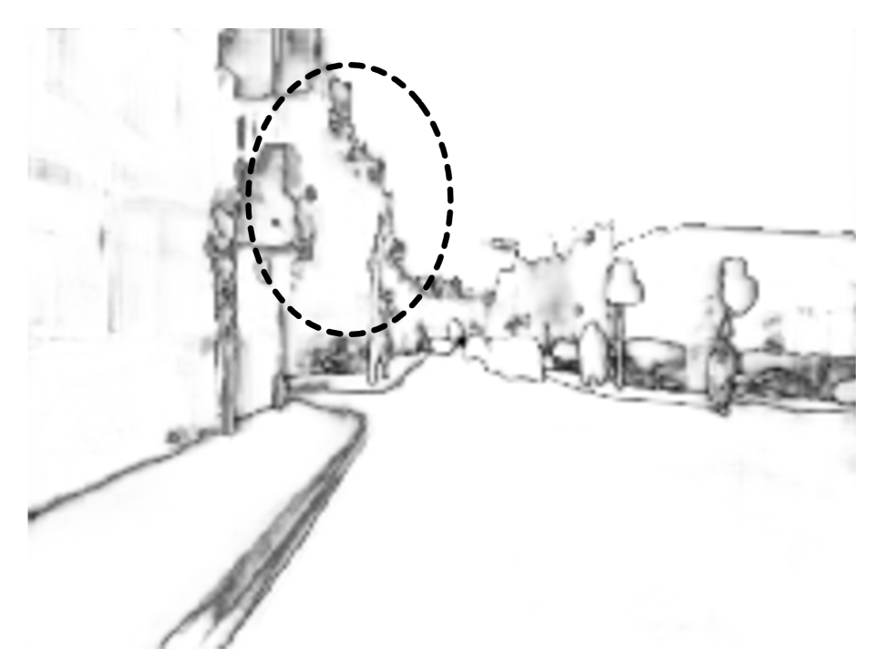


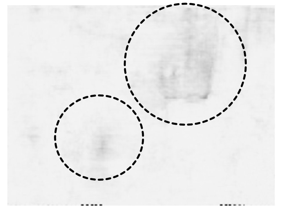


Figure 8 shows the qualitative comparison of the predictions for each method. In this figure, DNN is overconfident, i.e., confidence is high even when the prediction is wrong, and uncertainty is mostly distributed at the edge of the objects. The uncertainty of BNN is distributed on the edge as in the case of the DNN, but is also distributed in the misclassified areas. VQ-DNN is less overconfident compared to DNN. Also, although VQ-DNN does not identify all of the misclassifications compared to BNN, it sometimes estimates high uncertainty in the misclassified areas. The uncertainty of VQ-BNN is similar to the BNN as we expected. This figure is a comparison on a static image sequence; see Figure 4 for a comparison on a dynamic image sequence.
Edge predictive performance.
In Section 3.2, we argue that misclassification in semantic segmentation frequently occurs at the edge of the object, and VQ-BNN shows high predictive performance at the edge of the object. To demonstrate these, we propose edge predictive performance, which is the predictive performance for the pixel of the object edge. We use the Sobel operator to detect the object edge and find a pixel that satisfies the following conditions:
| (18) |
where and are the pixel-wise results of the Sobel operator of - and -coordinate for input image, respectively, and is non-negative threshold. For example, if is 0, all pixels will be edge pixels. We obtain the edge predictive performance by measuring the performance for the pixel corresponding to this condition.
Table 6 shows the edge predictive performance of each method when thresholds are 0.0, 0.5, and 1.0 in the case of CamVid & U-Net. The results of this table support our claims. See Section 3.2 for analysis on this table.
Temporal consistency.
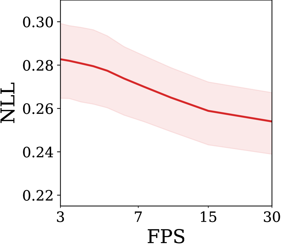
As described in Section 2, VQ-BNN relies on temporal consistency of data streams. To evaluate the sensitivity to the temporal consistency, we conduct an experiment of reducing frame rate, which decreases temporal consistency. In this experiment, we subsample 30fps CamVid image sequences every 2 to 10 frames; then, we evaluate VQ-BNN on these 3 to 15 fps video streams.
Figure 10 shows the NLL of VQ-BNN for the video frame rates. According to the result, when the frame rate is reduced, the predictive performance in terms of NLL is degraded. For the frame rate is 10fps or higher, VQ-BNN significantly improves the predictive performance, whereas for the frame rate is 5fps or less, it provides only a marginal performance improvement.
Improving performance by using future predictions.
Section 2 discusses that VQ-BNN improves predictive performance by using past predictions. Similarly, VQ-BNN allows us to improve predictive performance by using not only past predictions but also future predictions. For example, for a classification task such as semantic segmentation, Eq. 10 is modified as follows:
| (19) |
where is the number of future predictions. In other words, the predictive distribution is the sum of one prediction for the input data, past predictions, and future predictions.
Figure 11 shows the predictive performance of VQ-BNN in terms of NLL for the number of future frames with semantic segmentation on the CamVid. In this experiment, VQ-BNN uses 5 past predictions. According to the result, as increases until 5, the predictive performance improves.
In stream processing, VQ-BNN cannot estimate predictions for future inputs that are not given. Instead, VQ-BNN calculates the predictive distribution by using Eq. 19 after inputs are given. As a result, future predictions improves predictive performance, but increases latency. For example, if VQ-BNN uses one future frame to process 30fps video, the latency increases by 1/30 second. For this reason, we recommend using one or two future predictions in a practical situation.
D.2 Depth Estimation
Section 3.3 shows the performance of VQ-BNN with depth estimation. This section uses SegNet additionally, and provides detailed information and experimental results on this experiment.
Computational and predictive performances.
Table 5 shows the computational and predictive performance of various methods. We measure Bat Thr with batch size of 10. For other setups, we follow Section D.1.
We use additional metrics commonly used for depth estimation to measure predictive accuracy: mean relative error (Rel, ) and thresholded accuracies (, ). In the case of NYUDv2 & U-Net, all these metrics show that the predictive performance of VQ-BNN is the best. In the case of NYUDv2 & SegNet, the predictive performance of VQ-DNN and VQ-BNN are better then that of DNN and BNN, respectively. However, it might be an unusual result that VQ-DNN is better than VQ-BNN. The reason for the result is that DNN is better than BNN in this case.
| Method | Bat Thr (Img/Sec) | Str Thr (Img/Sec) | NLL | Acc (%) | Acc90 (%) | Unc90 (%) | IoU (%) | IoU90 (%) | Freq90 (%) | ECE (%) |
|---|---|---|---|---|---|---|---|---|---|---|
| DNN | 30.7 | 24.1 | 0.787 | 78.2 | 90.4 | 73.4 | 47.9 | 63.6 | 60.7 | 8.00 |
| BNN | 2.42 | 0.833 | 0.509 | 83.6 | 94.9 | 81.4 | 51.8 | 72.5 | 59.6 | 2.00 |
| VQ-BNN | 30.4 | 23.7 | 0.552 | 82.4 | 93.7 | 78.0 | 49.6 | 68.5 | 61.6 | 4.12 |
| AVP | 10.5 | 8.31 | 0.894 | 78.2 | 88.4 | 62.6 | 47.9 | 60.3 | 70.2 | 11.5 |
Qualitative results.
Figure 9 shows the qualitative comparison of the predictions for each method. DNN predicts uniform uncertainty in the regression task; the uncertainty estimated by DNN is meaningless. BNN estimates high uncertainty at the misestimation areas. In this example, NNs incorrectly estimate the depth of the corridor window, and BNN estimates high uncertainty at the window area. VQ-DNN does not exactly find out which results are incorrectly estimated, but exhibits high uncertainty at the object edge. Since it is difficult to estimate the depth of object edges, the predictive performance of VQ-DNN is better than that of DNN. VQ-BNN represents both types of the uncertainties, so the uncertainty of VQ-BNN is reliable.
Appendix E Comparison with Sampling-free BNN
As mentioned in Section 4, most sampling-free BNNs only work well for shallow NNs with several layers or less. (Postels et al. 2019) concurrently proposed Approximated Variance Propagation (AVP), and, to the best of our knowledge, it is the only sampling-free BNN with enough layers for practical tasks such as semantic segmentation. AVP transforms the trained BNN with MC dropout into an approximate neural network that predicts a Gaussian distribution with a diagonal covariance matrix. This section compares the performance of VQ-BNN and AVP.
In principle, if our understanding is correct, AVP is not designed for classification tasks such as semantic segmentation, and (Postels et al. 2019) did not provide a quantitative comparison with semantic segmentation experiment in the paper. Neural networks for semantic segmentation have to predict categorical distributions. However, the neural network transformed by AVP predicts the means and standard deviations of the Gaussian distribution, and standard deviations are not applicable to categorical distribution.
To solve this problem, we use a method to convert the standard deviations of the Gaussian distribution to the confidences of the categorical distribution. We follow the (Postels et al. 2019) and derive the standard deviation of BNN’s predictions. Subsequently, we generate a one-to-one correspondence between standard deviation and confidence based on the original BNN predictions. We only use Bayesian SegNet (Kendall, Badrinarayanan, and Cipolla 2015) in this experiment because (Postels et al. 2019) does not provide a transformation for skip layers. We follow (Postels et al. 2019) for other experimental setups.
Table 7 shows the quantitative comparison of DNN, BNN, VQ-BNN, and AVP, on the CamVid dataset. The results shows that the predictive result of AVP is more inaccurate than that of BNN and VQ-BNN, and is comparable to that of DNN. Moreover, AVP shows less accurate estimation of uncertainty than BNN and VQ-BNN. The throughput of AVP is 34 of that of DNN while the throughput of VQ-BNN is 98.
In conclusion, AVP has the following limitations: First, as (Postels et al. 2019) mentioned in the paper, “the magnitude of the approximated uncertainty (by AVP) is much lower than the sampling-based uncertainty”, i.e., AVP is not well-calibrated. To achieve high predictive performance, it seems essential to calibrate the results of AVP at a granular level. Second, AVP can transform a limited kind of neural network. AVP only deals with BNNs that contain noise injection layers such as MC dropout and layers for which the transformation rules are known. Third, AVP predicts only Gaussian distribution with diagonal covariance matrix. As in this section, AVP requires additional methods to convert standard deviations to apt uncertainty to solve discrete problems such as classification tasks. Finally, AVP is considerably slower than VQ-BNN because AVP predicts mean and standard variance separately.