Coverage Sampling Planner for UAV-enabled Environmental Exploration and Field Mapping
Abstract
Unmanned Aerial Vehicles (UAVs) have been implemented for environmental monitoring by using their capabilities of mobile sensing, autonomous navigation, and remote operation. However, in real-world applications, the limitations of on-board resources (e.g., power supply) of UAVs will constrain the coverage of the monitored area and the number of the acquired samples, which will hinder the performance of field estimation and mapping. Therefore, the issue of constrained resources calls for an efficient sampling planner to schedule UAV-based sensing tasks in environmental monitoring. This paper presents a mission planner of coverage sampling and path planning for a UAV-enabled mobile sensor to effectively explore and map an unknown environment that is modeled as a random field. The proposed planner can generate a coverage path with an optimal coverage density for exploratory sampling, and the associated energy cost is subjected to a power supply constraint. The performance of the developed framework is evaluated and compared with the existing state-of-the-art algorithms, using a real-world dataset that is collected from an environmental monitoring program as well as physical field experiments. The experimental results illustrate the reliability and accuracy of the presented coverage sampling planner in a prior survey for environmental exploration and field mapping.
I INTRODUCTION
Automated sensing systems that can carry out in-situ sampling, real-time processing, and remote deployment have been widely deployed in environmental monitoring programs. Although sensing systems with static sensors have been widely implemented to provide on-line measurements (e.g., [1, 2]), their applications have been impeded by the inadequacy and inflexibility in area surveillance. In contrast, unmanned aerial vehicles (UAVs) can offer flexibility, efficiency, and effectiveness in information gathering on the spatial scale. Consequently, UAV-enabled robotic sensors are being implemented in exploring and monitoring of environmental processes [3].
Depending on the monitoring goals, a UAV is equipped with appropriate sensors to measure the necessary variables/parameters (physical, chemical, biological, etc.). A specific type of sensor may be able to acquire data from multiple geographical locations simultaneously. For example, a thermal camera can capture the temperature distribution over a large spatial area. Many other types of sensors, however, may only acquire data from a single location at one time. For example, an air quality probe measures the target parameter concentration (e.g., PM2.5, CO, or SO2 [4]) at just one site at a time. These sensors are termed “point sensors” in the present paper. The measurements from them can provide the information pertaining to the corresponding sampling locations only. Then, to obtain the spatial information, the mobile sensing robots with point sensors have to navigate to sampling locations in the study area to take necessary measurements. The observations made in this manner are utilized to estimate the spatial field or predict the physical quantity of any unobserved locations.
Exploring and mapping an area of interest with point sensors have been actively studied in applications such as geostatistics, robotics, wireless sensor networks, and environmental monitoring. Observations from the sampled sites are utilized to characterize the spatial profile, estimate the underlying environmental model, predict the information at unobserved locations, or reconstruct the scalar field of the monitored area. Sites to be measured are generated following a sampling design, which affects the estimation and mapping performance. To investigate an unknown field of interest, a preliminary coverage sampling phase is required through a prior survey, which is called an exploratory survey phase [5]. A coverage sampling design is required that can distribute plots densely and evenly over the measured area. Subsequently, knowledge-based strategies and implementations can be further performed by using the gathered information.
In a UAV-enabled mobile sensing process, a robot navigates to different locations for carrying out automated sampling and data acquisition. It is evident that sampling at a higher resolution that covers the overall spatial field will provide estimations that are closer to the ground truth of the underlying environmental phenomenon. However, UAVs in the field have limited on-board resources, especially limited energy storage and power supply (batter, fuel, etc.), which restrict the number of collected data samples as well as the associated area of coverage. Accordingly, the major challenge for UAV-based sensing applications resides on how to schedule an effective and efficient sampling mission to visit and measure at different sites over the monitored area.
This paper presents a sampling planner for UAV-based mobile sensing that integrates both coverage sampling design and associated path planning for exploration and mapping of an unknown environment. The proposed scheduling framework generates a hexagonal grid-based sampling design that provides spatially balanced sampling sites and the sampling path cycle to visit them. The planned sampling mission results in an optimal coverage density for exploratory sampling, subject to a limited power supply budget. The robotic sensor travels along the assigned sampling path to collect data samples. Subsequently, the data is used to estimate a statistical model of the underlying environmental phenomenon in the form of a random field represented by a Gaussian process (GP) with a spatial trend. A robust Kriging method is utilized to estimate the GP structure and construct the scalar map of the monitored parameter. The experimental results are presented and compared with the existing approaches, while highlighting the superior performances of the proposed coverage sampling planner. The rest of the paper is organized as follows. Section II introduces the related work. In Section III, the problem formulation of the present work is addressed. The proposed mission planner for coverage sampling and path planning is detailed in Section IV. Section V presents the experiments and discusses the experimental results. The final section concludes the paper.
II Related Work
Environmental field estimation and mapping through mobile sensing is an active research topic. Model-based approaches have attracted attention of researchers for spatial data analysis since they can estimate the underlying structure of the data generating process and provide the spatial characteristics and global information of the environment. For example, by generalizing a Gaussian distribution in a finite vector space, to a Gaussian process in a function space of infinite dimension, the GP framework can be used to model various physical phenomena and estimate values at any location in the sensing domain [6].
A distribution of sampling locations provides a pattern across the study area, which indicates the estimation performance of the underlying field. Many frameworks have been proposed to select the target locations for constructing the scalar field. Among them, the experimental design theory has been studied to find the optimum sensor deployment plan by optimizing an information gain that is determined by using an established model. In the research, strategies were addressed to select the locations with high “informativeness” to achieve adaptive sensing (e.g., [7]). However, these strategies rely on prior knowledge of the environmental model structure. Deviations of the assumptions will lead to model misspecification and unacceptable estimation performance. In other words, the field estimation results will not be robust against misspecification of the established model. In many circumstances, the assumptions may not be practically feasible. For instance, the assumption of a known and constant mean of the environmental model (e.g., [8]) can cause inferior estimation performance in a practical situation where unknown spatial trends exist.
For an unknown environment, the underlying environmental model is learned by utilizing observations that are taken across the study area. Coverage sampling that is done to relax unrealistic assumptions is called an exploratory design, which provides sufficient flexibility to explore an unknown field [5]. Such designs have been adopted in spatial mapping without rigid prior assumptions, for initial collection of prior knowledge, exploratory survey for long-term design improvement, or combination with optimum designs for improved estimation performance. In most existing monitoring programs, the exploratory sampling is required to learn the underlying field. Regular grid-based sampling approaches accomplish such objectives as exploratory designs [9, 10]. These approaches distribute sampling sites by decomposing the field into a grid of cells (e.g., squares, triangles, hexagons) where the samples are taken in the grid tessellation. In the absence of prior knowledge, a regular grid ensures overall coverage of the surveillance area. In particular, it provides a simple frame to distribute spatially balanced data samples across the study area for prior survey.
For carrying out a sampling mission with a robotic sensor, a path to visit target sites is planned. The traveling salesman problem (TSP) [11] has been widely applied by connecting all the target locations directly. It finds the path by visiting each location exactly once and leads to the shortest route for mobile sensing. However, the TSP solvers are nondeterministic polynomial-time hard (NP-hard) [12]; thus the computational cost is extremely high for a large scale problem. Most critically, these methods do not provide freedom to iteratively adjust the sampling pattern for better estimation performance while ensuring that the cost of the resultant path does not exceed the available power. In contract, many other planners try to generate a coverage path first and then plot the samples along the path. In the literature, cellular decomposition methods, such as Boustrophedon path [13], lawnmower path [14], and their variants [15, 16], have been studied to generate a transect survey pattern consisting of a series of parallel linear transects to cover the study regions. Then data samples are taken while traveling back and forth along the generated coverage path. The work in [17] reviews the strategies that can plan a coverage path. Although these planners can generate coverage paths, most of them focus on the problem of sweeping over the area without analyzing the effect of the resulting sampling frames on spatial field mapping. Additionally, a constrained total travel length has not been addressed or emphasized in these planners.
To the best of our knowledge, scheduling of a UAV-enabled robotic sensor under an energy constraint in field exploration and mapping has not been adequately investigated. The present work introduces a scheme that integrates both coverage sampling design and path planning, which guides the sensing agent to take measurements for estimating and mapping an unknown environment more effectively. The proposed method can plan a path cycle with an optimal coverage density for sampling under a power supply budget.
III Problem Formulation
III-A Random Field & Environmental Model
Environmental phenomena are reflected by complex interactions of ecological processes. The variation of an environmental property appears to be random, which is commonly modeled as a random variable in spatial statistics. A set of random variables can be represented as a random field. The associated nomenclature of the present paper is given as follows. The region of interest is a 2-dimensional plane that is denoted by the set with its contour . The continuous plane is discretized as a set of locations with the possible sampling locations. Let denote a 2-dimensional coordinate vector of a sampling location in the surveyed field. A random field is a set of random variables indexed by its associated locations . A physical quantity can be observed from a random variable at its sampled location. In the present work, the random variable is represented by the model:
| (1) |
where is a regression function that defines the mean value of the process (spatial trend over space) and is a stochastic function that defines the random variation. Consider the finite random variables at the locations in , the model in Equation (1) is vectorized as:
| (2) |
Equation (2) represents the underlying environmental model.
To study the random field , it is required to take finite realizations at some sampled locations and make inferences on other unobserved random variables using these data samples and the environmental model. Given any set of sampled locations , the corresponding realizations are denoted as , referring to the set of observations at these locations.
III-B Sampling Design & Mobile Sensing Model
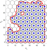
Statistical model and its characteristics of a random field are interpreted according to the distribution of sampling locations over the field. In the present work, a hexagonal grid framework is used to generate the locations of interest for coverage sampling and plan the associated coverage path. Specifically, the sensing domain of the continuous planar area is first decomposed into a grid of hexagonal cells. The cells that have their centroids within the study area are designated as the sub-regions of interest (SRoIs). These cell centroids are the sampling locations of interest (SLoIs), , for collecting data samples. An execution example of the proposed design of coverage sampling in a hexagonal tessellation is shown in Fig. 1(a).
In the sampling design, denotes the edge length of a hexagon in the grid; and and denote the point set and the total number of the generated SLoIs, respectively. In the context of mobile sensing with a UAV, let the sequence represent a planned path, where denotes a sampling location (waypoint) that is visited within the path . denotes the total path length. The UAV visits and operates the measuring process at the locations by following the order in the sequence. Let the set and represent the set and the number of sampling locations that are visited along this path, respectively. Let and represent the distance and energy cost when traveling from location to , respectively. In the measuring process, the UAV hovers at a SLoI to carry out the in-situ measurement using a point sensor. Let represent the energy consumption of the entire measurement process at a SLoI. The total energy cost of traveling along the path is expressed as:
| (3) |
The objective of the present planner is to generate a sampling mission for scheduling a UAV-enabled sensor to collect data samples at the target locations in with the densest sampling resolution under the power supply budget of the UAV. The data acquired in this manner can be utilized to estimate the underlying field model and map the scalar field . The objective is formulated as:
| (4) |
IV Coverage Sampling Planner
IV-A Coverage Path Planning
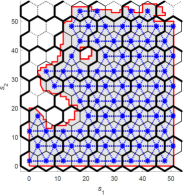
To carry out the sampling design, an ordered sequence is generated that indicates the sequential SLoIs to be visited. A coverage path is planned to visit each SLoI in the order of the sequence. This task is carried out by finding the effective edges (path segments) between the neighboring SLoI pairs to form the final path cycle. The edge candidates between the adjacent SLoIs compose a triangular grid pattern (see Fig. 1(b)). The planning goal is to determine the effective edges among the candidates to form a path cycle that visits each location only once and ends at the starting position.
To determine the effective edges, an auxiliary coarse cell (ACC) decomposition method is proposed. In this decomposition, each coarse cell contains four neighboring regular hexagons (fine cells). The target edges are constructed by examining the number and the positions of the SLoIs within and surrounding an ACC. An execution example of the edge candidates and the ACC decomposition is shown in Fig. 1(b).
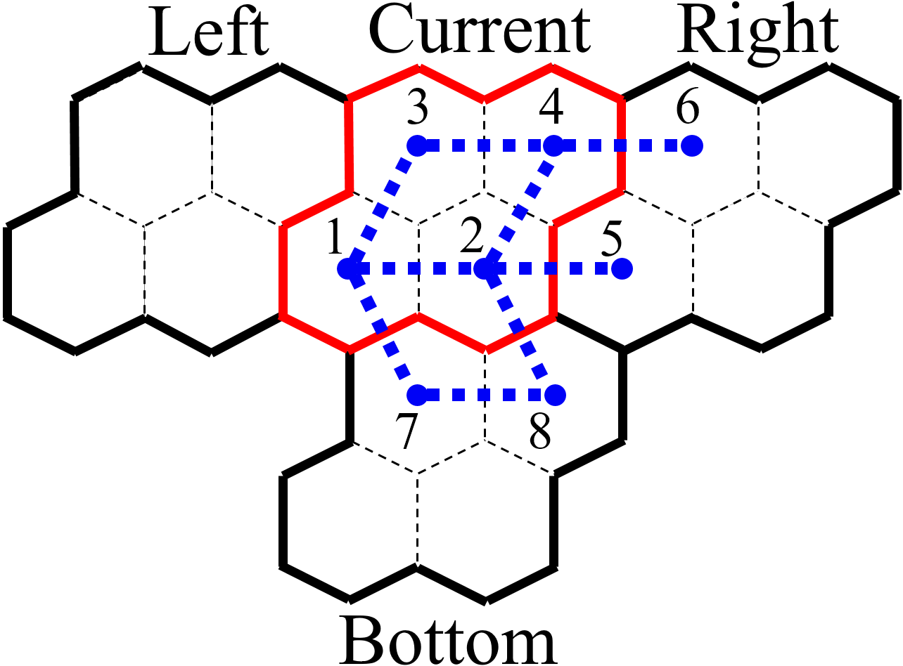
The proposed planner traverses the ACCs one by one to generate the path segments depending on the conditions (number and position) of the SLoIs in the current ACC and its surrounding ACCs. In a coarse cell, the bottom left, bottom right, top left, and top right hexagonal polygons are designated as the fine-cells 1, 2, 3, and 4, respectively. The current coarse cell is considered as a full cell if it contains four fine cells. The neighboring four fine cells in its right and bottom neighboring coarse cells are defined as the cells 5, 6 and cells 7, 8, respectively. The related SLoIs of an ACC for the path segment generation is shown in Fig. 2(a). In the figure, the SLoIs of the current and its neighboring coarse cells are labeled with the corresponding numbers. The dashed blue lines show the possible path segments to be generated. When traversing ACCs, for a selected coarse cell that is full, the segment paths are constructed by the following rules:
-
•
If the left neighboring ACC is full, generate the edge ; otherwise, generate the edges and .
-
•
If the right neighboring ACC is full, generate the edges and ; otherwise, generate the edge .
-
•
If the bottom ACC is full and the current ACC row has not been connected to the bottom ACC row, generate the edges and , and remove the existing edge ; otherwise, generate the edge .
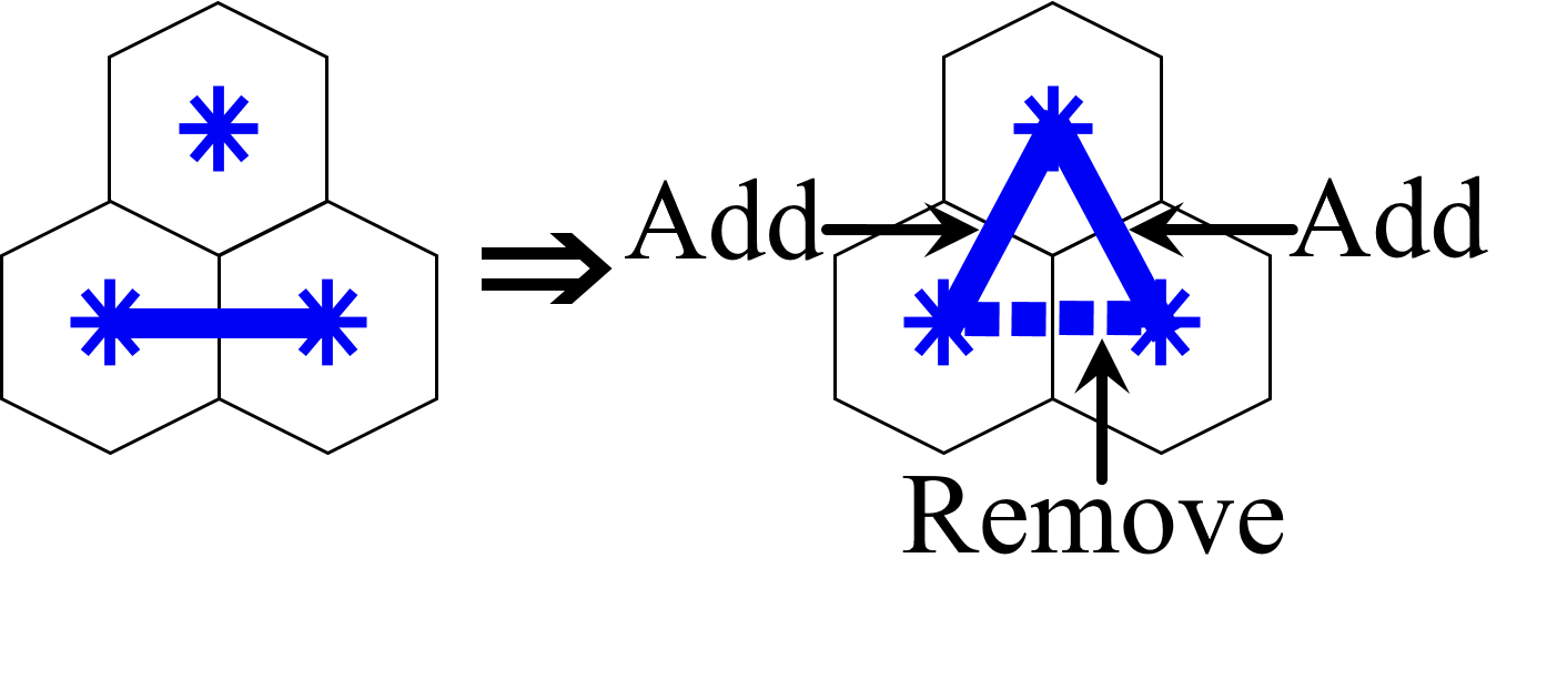
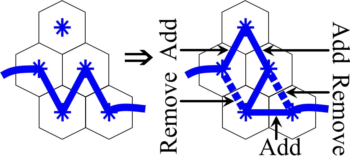
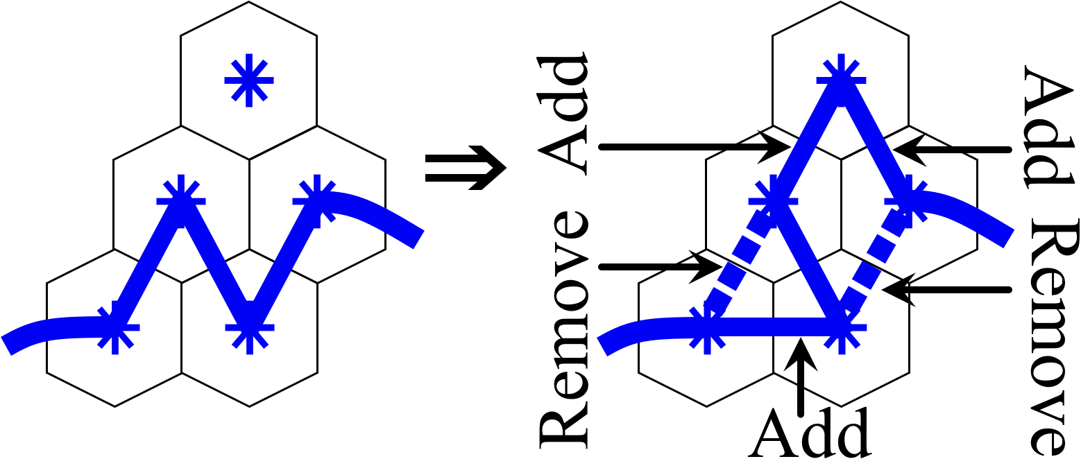
After executing these procedures, a path cycle is generated to visit all the full ACCs. However, there are still unvisited SLoIs within the area contour whose ACCs are not full. To visit them, several strategies for path segment generation are applied. First of all, for an unvisited SLoI, if there is a pair of neighboring SLoIs with a constructed edge between them, add two new edges connecting the current SLoI to the two neighbors, and then remove the edge between the neighbors (see Fig. 2(b)). In addition, if there are four neighboring SLoIs with two possible “Z” shaped patterns in Fig. 2(c), then the modification rules of the path segments are shown in the figure. The above-mentioned strategies are referred as the - and -modifications in the work of Arkin et al. [18]. The coverage path is updated by iteratively checking and implementing these strategies on all unvisited SLoIs. It is noted that the planned results may form more than one path cycle. Then, any two neighboring cycles can be combined to form one cycle by a simple edge adjustment (see Fig. 2(d)).
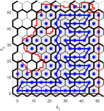
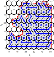
When compared with the work in [18], the proposed scheme is more robust for dealing with a triangular grid graph. The compared work requires that the planner starts from a boundary cycle of a 2-connected polygonal triangular grid. In contrast, the proposed method tackles the path cycle from inside to outside. There are no specific requirements on the characteristics of the input triangular grid graph. The proposed hexagonal grid-based coverage (HGC) sampling planner is summarized by the pseudo code in Algorithm 1. The code from line 1 to 21 generates the coverage path to visit all full ACCs. The code from line 22 to 32 deals with the unvisited ACCs. The algorithm generates a coverage path cycle to travel among the expected sampling sites. Fig. 3 shows the execution examples of the proposed method.

IV-B Optimal Sampling Density
The distances between any neighboring SLoI pairs are equal, which indicates the spatial sampling resolution. Given an edge length of the fine cells in the hexagonal grid, the distance is given by . For the area contour , the total number of SLoIs to by surveyed, , can be determined as a dependent variable of as well as . In view of the equal distances between SLoI pairs, the total path length of the generated coverage path can be determined as , . Given an energy budget , finding the maximum point set , , that the coverage path can achieve provides the most dense coverage sampling and further improves the exploration performance of field estimation and mapping. The optimal sampling density is determined by the optimal edge length as:
| (5) |
A decreasing grid spacing intuitively increases the resultant number of SLoIs, , inside the study area. However, there is no analytical expression for determining given , since the shape of the study area is generally irregular and complex. The dependent variable has to be determined by executing the ACC decomposition for a given . The optimal is chosen as the optimal coverage density of sampling to generate the final path. The efficiency of finding the optimal can be operated by using the binary search to determine such that .
The proposed planner guarantees that the total length of the generated path is bounded and indicative referring to the cell size. There is no need to execute the path generation algorithm before determining the optimal edge length . It considerably reduces the computational complexity and the corresponding processing time when finding the optimal coverage density. The coverage sampling path can be obtained by the planner in Algorithm 1. The proposed hexagonal grid-based coverage (HGC) sampling planner is summarized by the pseudo code in Algorithm 2.
IV-C Model Estimation & Field Mapping
The data samples taken along the planned path are used to estimate the underlying environmental model and build the field map. In the present work, the universal Kriging method [19] is implemented to estimate the unknown field. In the universal Kriging model, the regression function of the environmental model in Equation (2) is treated as a multivariate polynomial; that is:
| (6) |
where represents the basis function (e.g., the power base for a polynomial), represents the coefficients of the regression function. Meanwhile, the stochastic function in Equation (2) is modeled as a GP: with zero mean, variance , and a covariance function . The covariance function is also known as a kernel, describes the spatial dependence between the locations and , , where denotes the hyperparameters. As a result, the random field can be expressed as a GP: .
Given a set of samples with the corresponding observations , the prediction mean and variance are derived by utilizing the Kriging framework at the locations as follows:
| (7) | |||
| (8) |
where is the attribute matrix for , is derived by generalized least squares, defines the correlations between and the locations in , and .
Consider rare prior knowledge of the underlying field, the blind Kriging approach [20] is adopted in the present paper to identify the regression function. It makes approximation by extending the general universal Kriging model [19] with additional candidate functions in the regression analysis. The regression function is designated by unknown basis functions in the multivariate polynomial utilizing a Bayesian feature selection method; that is:
| (9) |
where denotes the set of candidate functions, and denotes the corresponding scores of the candidate functions. More details of the blind Kriging method are found in [21]. For the stochastic term, the Matérn 5/2 kernal is selected as the covariance function, which is expressed as:
| (10) |
where denotes the Euclidean distance between and , denotes the characteristic length-scale parameter. The hyperparameters are identified through the maximum likelihood estimation (MLE) [22]. In the next section, the performance of the proposed scheme is demonstrated through experiments.
V Experimental Results
This section presents the simulation and field tests by implementing the proposed method in field estimation and mapping. The proposed approach is also compared with the existing methods for coverage sampling design and path planning, including square grid-based spanning tree coverage (SGSTC) planner [23], discrete monotone polygonal partitioning-based (DMPP) planner [16], and hexagonal grid-based TSP (HGTSP) planner. The SGSTC method was originally designed for sweep coverage planning, which is adopted to coverage sampling for comparison in the experiment. The DMPP method, a variant of the Boustrophedon survey was designed to generate coverage path for sampling and field mapping. The HGTSP method utilizes the same sampling design as the present work but they plan the coverage path by a TSP solver. Note that in these methods different parameters are used to adjust the coverage density of sampling. Specifically, the edge length of a fine square cell is set to control the spacing in SGSTC. The distance between the spaced transects determines the spacing in DMPP. The edge length of a hexagonal cell defines the coverage density in HGTSP and HGC. These parameters are defined as the sampling density regulator (SDR) in the present experiments. Consequently, the optimal SDR (OSDR) is the corresponding parameter in Equation (5).
V-A Simulation
V-A1 Real-world dataset
In the simulation, a ground truth map over a surveillance area is chosen from a real-world dataset, NOAA operational model archive and distribution system (NOMADS) [24] provided by the National Oceanic and Atmospheric Administration (NOAA). The dataset records area measurements of surface salinity of the Caribbean Sea using a radiometer. In the dataset, an estuary area (latitude: 28.4339N-30.4155N, longitude: 87.6968W-89.7512W) with apparent spatial variation is chosen as the study area to evaluate the performance of the planners. A ground truth map is shown in Fig. 5(a), where the colors indicate the surface salinity concentrations in units of psu.
V-A2 Mapping performance
The mapping performance is evaluated by comparing the prediction values with the ground truth values at the unobserved locations. The root mean square error (RMSE) and the average Kriging variance (AKV) are utilized as measures to determine the mapping performance, which are defined as:
| (11) |
where denotes the set of grid nodes for spatial interpolation, , denotes the element number of the set, and denotes the ground truth value at locations . A smaller RMSE indicates a more accurate prediction at the unobserved locations of the field. A smaller AKV indicates a lower estimation uncertainty.
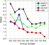
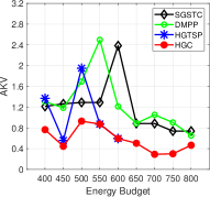
The power supply budget determines the total distance a mobile robot can travel. For simplicity, the budget is designated in a unit of length rather than energy in the simulation. To investigate the mapping performance with respect to the power constraint, different energy budgets are assigned when planning the sampling paths. Fig. 4 shows the simulation results of the compared methods with respect to the different energy budgets. For brevity, some OSDR and field mapping results are presented in Table I and displayed in Fig. 5. The configuration of the binary search for the OSDR is set as , , , and , .
| Budget | Metric | SGSTC | DMPP | HGTSP | HGC |
|---|---|---|---|---|---|
| 5.36 | 5.52 | 4.74 | 4.58 | ||
| 400 | 2.8272 | 2.2149 | 1.7870 | 1.7960 | |
| 1.2134 | 1.3072 | 1.3704 | 0.7662 | ||
| 4.51 | 4.84 | 3.78 | 3.68 | ||
| 500 | 2.5179 | 1.9065 | 2.1930 | 1.4064 | |
| 1.2907 | 1.6925 | 1.9507 | 0.9302 | ||
| 4.05 | 4.16 | 3.10 | 3.10 | ||
| 600 | 1.9496 | 1.4642 | 1.1765 | 1.1765 | |
| 2.3832 | 1.2136 | 0.5967 | 0.5967 | ||
| 3.76 | 3.68 | N/A | 2.91 | ||
| 700 | 1.6517 | 1.4064 | N/A | 1.1358 | |
| 0.8850 | 1.0521 | N/A | 0.2921 | ||
| 3.25 | 3.35 | N/A | 2.51 | ||
| 800 | 1.7153 | 1.6199 | N/A | 0.9214 | |
| 0.7389 | 0.6521 | N/A | 0.4666 |
N/A: Execution did not complete within the time limit of 15 min.
Grey color highlights the best prediction results.
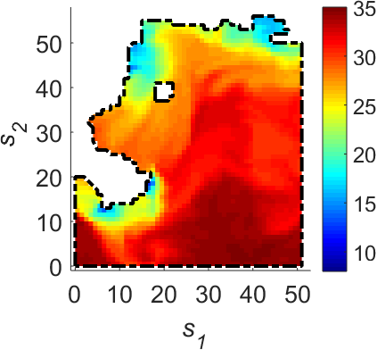
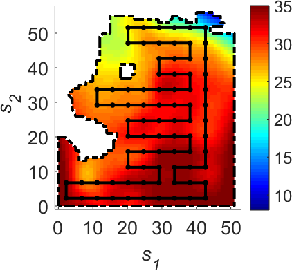
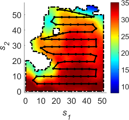
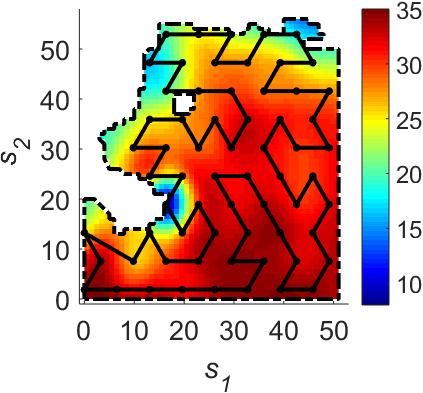
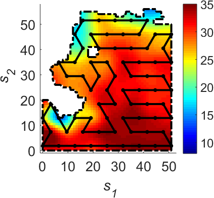
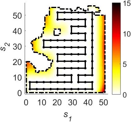
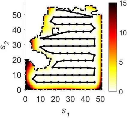
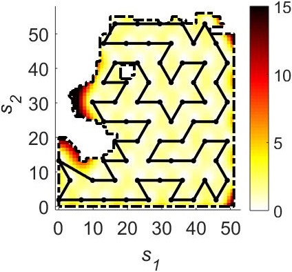
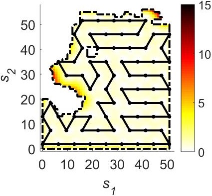
As clear from Fig. 4 and Table I, the proposed method provides more accurate results of field estimation and mapping when compared with the other approaches, as expressed by the RMSE and the AKV results with different power supply budgets. In the limited number of simulation results, the HGTSP method may provide the lowest RMSE. However, for a larger sampling density, the HGTSP methods were unable to find a plan due to its NP-hard solution. In Fig. 5, the figures display the sampled locations, the generated coverage path, and the mapping results by making use of the observations at the sampled sites. The solid black dots and lines denote the planned SLoIs and the sampling paths, respectively. The colors in Fig. 5(b)-(e) indicate the corresponding predicted values at the unobserved locations in the study area. The colors in Fig. 5(f)-(i) display the corresponding estimated Kriging variances at the unobserved locations, which indicate estimation uncertainty in the monitored field. Fig. 5 demonstrate that the HGC method outperforms the other sampling planners on field estimation and mapping.
V-B Field Tests
The proposed planner was further evaluated by physical field tests. It was implemented on a UAV-enabled mobile sensor for aquatic environmental monitoring. The mobile sensor was built upon a DJI Phantom 4 quadrotor with a Libelium Waspmote board and a Raspberry Pi 3 microcomputer mounted on the UAV for data acquisition and onboard processing, respectively. A conductivity probe was equipped to measure electrical conductivity of water source in an in-situ manner, which connected to the data acquisition board to provide scalar readings with units of S/cm. The system has been deployed at the Yosef Wosk Reflecting Pool, which is a natural pool at University of British Columbia, Canada. The UAV-enabled mobile sensor and the study area of the monitored aquatic environment are shown in Fig. 6.
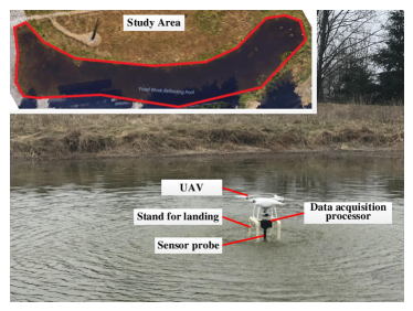
In each field test, one UAV was implemented by applying one of the planners to carry out the corresponding sampling mission. Meanwhile, another UAV was deployed to collect data at some unobserved locations, which was used as a validation dataset to evaluate the performance of field estimation and mapping. The fully charged battery (81.3 Wh) enabled the USV to fly for roughly 20 minutes at the average speed of 1 m/s. The hovering time for carrying out a measurement at each target location was set to 10 seconds (energy cost of about 2 Wh). The mapping results of the different planners were based on the underlying environmental models that were learned by the observations from the first UAV. The measurements taken by the second UAV were utilized as the ground truth to validate the mapping results.
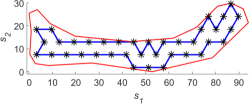
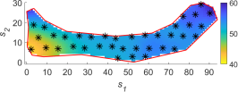
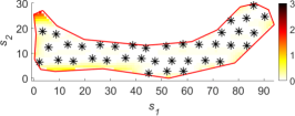
Table II shows the performance of the RMSE and AKV by implementing the proposed and compared planners. The proposed planner demonstrated its superior prediction performance compared to the other planners. To further display the mapping results, Fig. 7 provides the planning, prediction, and estimation results at the monitored pool by making use of the observations from the generated HGC sampling planner. The experimental results of the field tests further validated the conclusion in the numerical simulation that the proposed planner outperforms the state-of-the-art methods on environmental field estimation and mapping.
| Metric | SGSTC | DMPP | HGTSP | HGC |
|---|---|---|---|---|
| 2.5155 | 1.0760 | 0.6821 | 0.6754 | |
| 1.4196 | 0.8083 | 0.1961 | 0.1072 |
VI CONCLUSIONS
In the present paper, a hexagonal grid-based coverage sampling planner was proposed for spatial exploration, random field estimation, and environmental mapping. The proposed planning strategies provided a reliable and efficient coverage sampling mission for USV-enabled mobile sensing with a in-situ sensor, to make an effective prior survey of an unknown environment under a power constraint. The proposed planner could distribute coverage sampling densely and evenly across the overall study area while generating the corresponding coverage path to visit the target sampling sites. The experimental results on the real-world dataset and field tests validated the planner performance on mapping accuracy. In practical applications, the proposed scheme satisfies many circumstances in environmental monitoring, such as building an field map of an unknown environment, scheduling an initial deployment to gather sufficient useful information that can be exploited for further implementation or long-term monitoring. In future work, since the planned sampling path forms a path cycle, it can be divided into multiple optimal sub-paths to schedule multiple robotic sensors for sensing according to their power supply conditions.
References
- [1] S. Fang, L. Da Xu, Y. Zhu, J. Ahati, H. Pei, J. Yan, and Z. Liu, “An integrated system for regional environmental monitoring and management based on internet of things,” IEEE Transactions on Industrial Informatics, vol. 10, no. 2, pp. 1596–1605, 2014.
- [2] G. Mois, S. Folea, and T. Sanislav, “Analysis of three iot-based wireless sensors for environmental monitoring,” IEEE Transactions on Instrumentation and Measurement, vol. 66, no. 8, pp. 2056–2064, 2017.
- [3] M. Dunbabin and L. Marques, “Robots for environmental monitoring: Significant advancements and applications,” IEEE Robotics & Automation Magazine, vol. 19, no. 1, pp. 24–39, 2012.
- [4] Y. Yang, Z. Zheng, K. Bian, L. Song, and Z. Han, “Real-time profiling of fine-grained air quality index distribution using uav sensing,” IEEE Internet of Things Journal, vol. 5, no. 1, pp. 186–198, 2018.
- [5] W. G. Müller, Collecting spatial data: optimum design of experiments for random fields. Springer Science & Business Media, 2007.
- [6] Y. Xu, J. Choi, S. Dass, and T. Maiti, Bayesian prediction and adaptive sampling algorithms for mobile sensor networks: Online environmental field reconstruction in space and time. Springer, 2015.
- [7] L. V. Nguyen, S. Kodagoda, R. Ranasinghe, and G. Dissanayake, “Adaptive placement for mobile sensors in spatial prediction under locational errors,” IEEE Sensors Journal, vol. 17, no. 3, pp. 794–802, 2017.
- [8] W. C. Evans, D. Dias, S. Roelofsen, and A. Martinoli, “Environmental field estimation with hybrid-mobility sensor networks,” in Robotics and Automation (ICRA), 2016 IEEE International Conference on. Ieee, 2016, pp. 5301–5308.
- [9] L. Paull, S. Saeedi, M. Seto, and H. Li, “Sensor-driven online coverage planning for autonomous underwater vehicles,” IEEE/ASME Transactions on Mechatronics, vol. 18, no. 6, pp. 1827–1838, 2013.
- [10] M. J. De Smith, M. F. Goodchild, and P. Longley, Geospatial analysis: a comprehensive guide to principles, techniques and software tools. 5th ed. Winchelsea Press, 2015.
- [11] D. L. Applegate, The traveling salesman problem: a computational study. Princeton university press, 2006.
- [12] G. Gutin and A. P. Punnen, The traveling salesman problem and its variations. Springer Science & Business Media, 2006, vol. 12.
- [13] C. Fang and S. Anstee, “Coverage path planning for harbour seabed surveys using an autonomous underwater vehicle,” in OCEANS 2010 IEEE-Sydney. IEEE, 2010, pp. 1–8.
- [14] T. Somers and G. A. Hollinger, “Human–robot planning and learning for marine data collection,” Autonomous Robots, vol. 40, no. 7, pp. 1123–1137, 2016.
- [15] A. Mora, C. Ho, and S. Saripalli, “Analysis of adaptive sampling techniques for underwater vehicles,” Autonomous Robots, vol. 35, no. 2-3, pp. 111–122, 2013.
- [16] T. Wilson and S. B. Williams, “Adaptive path planning for depth-constrained bathymetric mapping with an autonomous surface vessel,” Journal of Field Robotics, 2017.
- [17] E. Galceran and M. Carreras, “A survey on coverage path planning for robotics,” Robotics and Autonomous systems, vol. 61, no. 12, pp. 1258–1276, 2013.
- [18] E. M. Arkin, S. P. Fekete, K. Islam, H. Meijer, J. S. Mitchell, Y. Núñez-Rodríguez, V. Polishchuk, D. Rappaport, and H. Xiao, “Not being (super) thin or solid is hard: A study of grid hamiltonicity,” Computational Geometry, vol. 42, no. 6-7, pp. 582–605, 2009.
- [19] N. Cressie, Statistics for spatial data. John Wiley & Sons, 2015.
- [20] V. R. Joseph, Y. Hung, and A. Sudjianto, “Blind kriging: A new method for developing metamodels,” Journal of mechanical design, vol. 130, no. 3, p. 031102, 2008.
- [21] I. Couckuyt, A. Forrester, D. Gorissen, F. De Turck, and T. Dhaene, “Blind kriging: Implementation and performance analysis,” Advances in Engineering Software, vol. 49, pp. 1–13, 2012.
- [22] C. M. Bishop, Pattern recognition and machine learning. Springer-Verlag New York, 2006.
- [23] A. C. Kapoutsis, S. A. Chatzichristofis, and E. B. Kosmatopoulos, “Darp: Divide areas algorithm for optimal multi-robot coverage path planning,” Journal of Intelligent & Robotic Systems, vol. 86, no. 3-4, pp. 663–680, 2017.
- [24] NOAA. (2018) Noaa operational model archive and distribution system (oceannomads) @ONLINE. [Online]. Available: http://ecowatch.ncddc.noaa.gov/