Time delay estimation in satellite imagery time series of precipitation and NDVI: Pearson’s cross correlation revisited

Abstract.

In order to describe more accurately the time relationships between daily satellite imagery time series of precipitation and NDVI we propose an estimator which takes into account the sparsity naturally observed in precipitation. We conducted a series of simulation studies and show that the proposed estimator’s variance is smaller than the canonical’s (Pearson-based), in particular, when the signal-to-noise ratio is rather low. Also, the proposed estimator’s variance was found smaller than the canonical’s one when we applied them to stacks of images (2002-2016) taken on some ecological regions of Mexico. Computations for this paper are based on functions implemented in our new R package geoTS (available here).

1. Introduction and Dataset

Time delay estimation consists of approximating the apparent shift between an emmited signal (also known as reference signal) and another one which is received in a different point in time and space (delayed signal).

Estimating this apparent delay between general signals has been a subject of study in fields as diverse as time series (Hamon and Hannan, (1974), Hannan and Thomson, (1988)), signal processing (Knapp and Carter, (1976), Carter, (1981)), radar, sonar and seismology Benesty et al., (2004), and remote sensing. Indeed, considering time series of satellite imagery as discretized signals, Vicente-Serrano et al., (2013), Barbosa et al., (2015) and Colditz et al., (2017), among others, have conducted global and regional studies seeking to determine the time relations between precipitation and vegetation growth (described, e.g. by the NDVI, which will also be used here). Naturally, precipitation is a sparse variable, that is, it may have prolonged periods of dry days (zero precipitation), and this characteristic has not been taken into consideration in the aforementioned studies.

In this paper we revisit the canonical tool to estimate the delay between discrete signals, the Pearson’s product moment association and propose to incorporate the precipitation’ sparsity, through solving a LASSO regression problem, in determining the delay. The resulting time delay estimator ($\mathsf{TDE}$) has proven to reduce the variance of the canonical estimator in many cases, see Section 3 for several simulation studies.

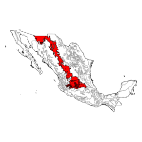
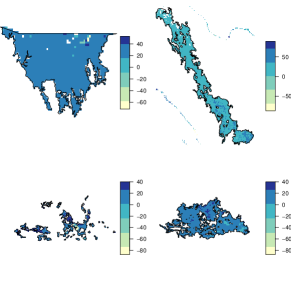
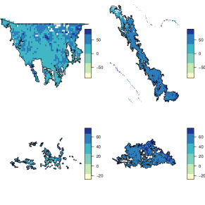
We have applied our approach to daily time series of precipitation and NDVI (from 2002 to 2016) taken on the Semi-arid Southern Uplands eco-region located in the Mexican Territory, see Fig.1. This eco-region is comprised by areas whose precipitation and vegetation show similar dynamics although they may include more than one ecosystem, cf. Ch.3 p.104 of CONABIO, (2008). This feature adds variability to any $\mathsf{TDE}$ and to the best of our knowledge an assessment of this variability still remains elusive and is one of the contributions of this work, see Section 4.

We utilize the Climate Hazards Group InfraRed Precipitation with Station (CHIRPS) dataset (ver. 2.0), see Funk et al., (2015). The NDVI used in this paper was derived from NASA’s product MCD43C4 (ver.6), cf. Schaaf and Wang, (2015). The spatial resolution of these two products is $0.05^{\circ}$. We re-sampled the eco-region shapefile, available online INEGI-CONABIO-INE, (2007), so that its spatial resolution coincide with the other two.

Notation: An $l$-dimensional vector full with zeros will be denoted as $\boldsymbol{0}_{l}$; for a generic vector we write ${\boldsymbol{v}}_{[i:j]}=\begin{pmatrix}v_{i},\ldots,v_{j}\end{pmatrix}^{\top}$, $i<j$.

[figure]style=plain, subcapbesideposition = top

[][][]

Figure 1. (A) Semiarid Southern Uplands eco-region (red). (B) Median of significant (at 5%) $\textnormal{LASSO}^{\tt CV}_{\tt trim}$ time delay estimates obtained from satellite imagery time series of daily precipitation and NDVI from 2002 to 2016 in regions (highlighted in (A), from top-left to bottom-right) Madrense, Mezquital, Interior Plains and Plateau Plains. (C) Median of significant (at 5%) ${\bf Pn}$ time delay estimates obtained from same products, time and regions described in (B).

2. Methodology

Let us introduce the time delay estimation problem based on the Pearson’s product moment association function. Let ${\boldsymbol{x}}=(x_{1},\ldots,x_{n})^{\top}$ and ${\boldsymbol{y}}=(y_{1},\ldots,y_{n})^{\top}$ denote the time series of precipitation and vegetation index, respectively; $n$ denotes the sample size. Let $\mathcal{G}_{n}$ denote the grid of $2n-1$ points $\{-(n-1),\ldots,-1,0,1,\ldots,n-1\}$. For $l\in\mathcal{G}_{n}$ the general Pearson’s product moment association between $\boldsymbol{x}$ and $\boldsymbol{y}$ is defined as

$$~{}\gamma_{l}=\begin{cases}\frac{1}{n-|l|}\,\sum_{k=1}^{n-|l|}\,M(x_{|l|+k};{\boldsymbol{x}})\,M(y_{k};{\boldsymbol{y}}),&l<0\\ \frac{1}{n-l}\,\sum_{k=1}^{n-l}\,M(x_{k};{\boldsymbol{x}})\,M(y_{k+l};{\boldsymbol{y}}),&l\geq 0\end{cases},$$ (1)

where $M(x_{k};\boldsymbol{x})$ can be equal to either $x_{k}$ (unscaled), $(x_{k}-\bar{\boldsymbol{x}})/\widehat{\sigma}_{\boldsymbol{x}}$ (standard) or $(x_{k}-\bar{\boldsymbol{x}}_{trim})/\widehat{\sigma}_{\boldsymbol{x}}^{trim}$ (trimmed). Above, $\bar{\boldsymbol{x}}$ and $\widehat{\sigma}_{\boldsymbol{x}}$ are the arithmetic mean and a standard deviation (s.d.) estimate of ${\boldsymbol{x}}$. Similarly, $\bar{\boldsymbol{x}}_{trim}$ and $\widehat{\sigma}_{\boldsymbol{x}}^{trim}$ denote mean and s.d., respectively, of $\boldsymbol{x}_{[(|l|+1):n]}$ for $l<0$ or $\boldsymbol{x}_{[1:(n-l)]}$ for $l\geq 0$. This generality in the computation of the empirical product mean between ${\boldsymbol{x}}$ and ${\boldsymbol{y}}$ allows us to study Pearson’s correlation and other popular forms of association considered in the literature of the time delay problem. In what follows we will assume that ${\boldsymbol{x}}$ and ${\boldsymbol{y}}$ have been standardized.

Let $\boldsymbol{\Gamma}=\begin{pmatrix}\gamma_{-(n-1)},\ldots,\gamma_{-1},\gamma_{0},\gamma_{1},\ldots,\gamma_{n-1}\end{pmatrix}^{\top}$. Note that (1) can be written in a matricial form. Indeed,

$$~{}\boldsymbol{\mathcal{S}}^{\top}\,\boldsymbol{x}=\boldsymbol{J}_{n}\,\boldsymbol{\Gamma},$$ (2)

where $\boldsymbol{J}_{n}$ is a $2n-1$ squared diagonal matrix with main diagonal equal to $(1,2,\ldots,n-1,n,n-1,\ldots,2,1)$ and $\boldsymbol{\mathcal{S}}\in\mathbb{R}^{n\times(2n-1)}$ is the sparse matrix whose $i$-th column is,

$$\boldsymbol{\mathcal{S}}[\cdot,i]=\begin{cases}\boldsymbol{a}_{i,n}^{\top}&1\leq i\leq n,\\ \boldsymbol{b}_{i,n}^{\top}&n+1\leq i\leq 2n-1\end{cases},$$

$\boldsymbol{a}_{i,n}=(\boldsymbol{0}_{n-i},\boldsymbol{y}_{[1:i]})$ and $\boldsymbol{b}_{i,n}=(\boldsymbol{y}_{[(i+1-n):n]},\boldsymbol{0}_{i-n})$. The $\mathsf{TDE}$ between ${\boldsymbol{x}}$ and ${\boldsymbol{y}}$ is by definition,

$$~{}\widehat{l}_{n}=\mathsf{argmax}_{l\in\mathcal{G}_{n}}\,{\gamma}_{l}^{2}.$$ (3)

In the last two decades the least absolute shrinkage and selection operator (LASSO) has been applied to myriads of practical problems in a wide range of the sciences, cf. Tibshirani, (2011). Now we argue that this operator can be used in the context of time delay estimation and, as it is shown in our simulations, the use of LASSO improves the precision of the resulting $\mathsf{TDE}$. In a nutshell, LASSO is regression with an $\ell_{1}$-norm penalty and this constraint induces sparsity in the estimated coefficients of the regression, i.e., the LASSO solution is a vector with a fair amount of entries which are identically zero. Although ${\boldsymbol{x}}$ is already a sparse vector, as it contains measurements of a precipitation process, we argue that by fitting a LASSO regression we can write ${\boldsymbol{x}}$ in a far more sparse representation and this will ease the solution of (3). Namely, we assume that there exists a highly sparse vector ${\boldsymbol{s}}\in\mathbb{R}^{2n-1}$, such that

$$\boldsymbol{x}=\boldsymbol{\mathcal{S}}{\boldsymbol{s}}+{\boldsymbol{\varepsilon}},$$

where ${\boldsymbol{\varepsilon}}=\begin{pmatrix}\varepsilon_{1},\ldots,\varepsilon_{n}\end{pmatrix}^{\top}$ contains error terms (possibly correlated). Then, we seek a vector $\boldsymbol{s}_{\ell_{1}}\in\mathbb{R}^{2n-1}$, which minimizes the penalized least squares problem

$$\sum_{i=1}^{n}(x_{i}-{\boldsymbol{\mathcal{S}}}[i,\cdot]\boldsymbol{s})^{2}+\lambda_{n}\sum_{j=1}^{2n-1}|s_{j}|,$$ (4)

for a given tuning parameter $\lambda_{n}$. Having determined $\boldsymbol{s}_{\ell_{1}}$, let $\widetilde{\boldsymbol{x}}=\boldsymbol{\mathcal{S}}\boldsymbol{s}_{\ell_{1}}$ and plug it into (1) to produce a new $\mathsf{TDE}$. That is, in this paper we propose

$$~{}\widetilde{l}_{n}=\mathsf{argmax}_{l\in\mathcal{G}_{n}}\,{\gamma}_{l}^{2}(\widetilde{\boldsymbol{x}},{\boldsymbol{y}})$$ (5)

as an estimator which takes into account the sparse nature of the original precipitation process ${\boldsymbol{x}}$.

2.1. On the penalization parameter

In order to solve (4) we need to provide a tuning parameter $\lambda_{n}$. Note that the larger the value of $\lambda_{n}$ the more sparsity we impose in the solution $\boldsymbol{s}_{\ell_{1}}$ so that this parameter must be carefully selected to avoid an overpenalization leading to meaningless estimators, e.g. the vector zero as the new representation of ${\boldsymbol{x}}$.

The standard algorithm to solve (4) provides an entire solution path (a set of values for $\lambda_{n}$ and its corresponding LASSO estimate), cf. Efron et al., (2004). As leave-one-out cross validation produces a tuning parameter whose LASSO estimate achieves the least predictive error we suggest its use to select $\lambda_{n}$. Another, less time consuming, empirical strategies will be discussed in Section 3.

2.2. On the search grid

We introduced problems (3)-(5) considering the general grid $\mathcal{G}_{n}$ but it is not recommended to optimize $\gamma_{l}^{2}$ over the entire grid. Indeed, note that at the left and right extremes of $\mathcal{G}_{n}$, $\gamma_{l}^{2}$ exhibits a great fluctuation as at those extremes only a small amount of observations are used to calculate the association between ${\boldsymbol{x}}$ and ${\boldsymbol{y}}$. Therefore it is common to utilize a smaller grid to solve (3) or (5).

In studies involved in assessing the time relationships between daily precipitation and vegetation growth, over a year, a grid of $\pm 3$ months has been used, e.g. Vicente-Serrano et al., (2013) and Barbosa et al., (2015); effectively, this represents to using only 25% of $\mathcal{G}_{n}$. In our applications we used grids of $\pm 2$, $\pm 3$ and $\pm 4$ months without finding major differences between the estimates. See Section 3.4 for comments on the relationship of signal-to-noise ratio ($\mathsf{SNR}$) and grid length.

3. Simulations

In this section we assess the performance of the $\mathsf{TDE}$s proposed in Section 2. Now we introduce notation for each of the methods under comparison.

$\boldsymbol{\vartheta}_{\tt option}^{\tt type}$ denotes a $\mathsf{TDE}$ in which the association function and tuning parameter are settled by ${\tt option}$ and ${\tt type}$, respectively. We used $\boldsymbol{\vartheta}=({\bf Pn},\textnormal{LASSO})$, i.e., a Pearson-based (via (3)) or a LASSO-based (via (5)) estimator. For ${\tt option}$ we consider trim and standard, see (1); the unscaled case is also consider (we simply leave a blank space). When ${\tt type}=0.1$ we selected the $10\%$ quantile of the tuning parameter ($\lambda_{n}$) distribution (a very fast procedure) and when ${\tt type=CV}$ we used $\lambda_{n}$ provided by cross validation. Each simulation setup will be repeated 1,000 times and we assess the behavior of these estimators through their mean and s.d.

3.1. Simulation of the precipitation process

In order to simulate easily a realistic daily precipitation time series of arbitrary length we use an occurrence and amount model. We simulate occurrences through a discrete Markov chain model with 2 states (dry day / wet day). In order to implement this model we need estimates of matrices of transition probabilities; further details are given below. We simulate rainfall amount from an exponentially distributed random variable (r.v.) as this is known to be appropriate and allows us to assess the performance of $\mathsf{TDE}$s as a function of the $\mathsf{SNR}$. Now we explain how we estimate the necessary parameters to execute our simulations.

$\mathsf{TDE}$s	$\tau=37$				$\tau=110$				$\tau=183$
	Exp($\lambda$) errors				Exp($\lambda$) errors				Exp($\lambda$) errors
	$\lambda=0.125$	$\lambda=0.5$	$\lambda=2.5$		$\lambda=0.125$	$\lambda=0.5$	$\lambda=2.5$		$\lambda=0.125$	$\lambda=0.5$	$\lambda=2.5$
Madrense
${\bf Pn}$	37.001 (0.032)	37.108 (0.524)	38.55 (3.516)		110.001 (0.032)	110.045 (0.315)	110.903 (2.164)		183 (0)	182.998 (0.045)	182.981 (0.25)
${\bf Pn}_{\tt trim}$	37 (0)	38.01 (10.3)	40.97 (18.586)		110 (0)	110.001 (0.152)	110.038 (1.335)		183 (0)	182.992 (0.089)	181.695 (18.586)
${\bf Pn}_{\tt standard}$	37 (0)	37.062 (0.395)	38.068 (5.473)		110 (0)	110.02 (0.199)	110.142 (1.396)		183 (0)	182.996 (0.063)	182.944 (0.464)
$\textnormal{LASSO}^{0.1}$	37 (0)	37.047 (0.345)	38.532 (3.504)		110 (0)	110.019 (0.197)	110.886 (2.098)		183 (0)	182.996 (0.063)	182.982 (0.248)
$\textnormal{LASSO}_{\tt trim}^{0.1}$	37 (0)	37.012 (0.189)	50.383 (34.935)		110 (0)	109.993 (0.114)	110.01 (1.177)		183 (0)	182.992 (0.089)	182.882 (0.876)
$\textnormal{LASSO}^{{\tt CV}}$	37 (0)	37.099 (0.497)	38.405 (3.374)		110.001 (0.032)	110.045 (0.315)	110.811 (2.085)		183 (0)	182.998 (0.045)	182.978 (0.279)
$\textnormal{LASSO}^{\tt CV}_{\tt trim}$	37 (0)	37.342 (5.967)	39.505 (14.78)		110 (0)	109.993 (0.114)	109.986 (1.072)		183 (0)	182.993 (0.083)	182.89 (0.82)
Mezquital
${\bf Pn}$	37 (0)	37.007 (0.217)	37.469 (3.58)		110.003 (0.055)	110.171 (0.671)	111.499 (3.366)		183 (0)	182.998 (0.045)	182.932 (0.337)
${\bf Pn}_{\tt trim}$	37 (0)	41.772 (22.373)	48.541 (33.669)		110 (0)	110.02 (0.286)	110.394 (2.444)		183 (0)	182.97 (0.182)	182.079 (11.197)
${\bf Pn}_{\tt standard}$	37 (0)	36.983 (0.207)	39.332 (16.903)		110 (0)	110.054 (0.333)	110.588 (2.466)		183 (0)	182.991 (0.094)	182.829 (0.736)
$\textnormal{LASSO}^{0.1}$	37 (0)	36.985 (0.225)	37.462 (3.573)		110 (0)	110.045 (0.295)	111.489 (3.301)		183 (0)	182.994 (0.077)	182.936 (0.341)
$\textnormal{LASSO}_{\tt trim}^{0.1}$	37 (0)	36.971 (0.224)	67.231 (48.797)		110 (0)	110.003 (0.239)	110.179 (2.025)		183 (0)	182.973 (0.174)	182.711 (1.098)
$\textnormal{LASSO}^{{\tt CV}}$	37 (0)	37.005 (0.207)	37.329 (2.878)		110.003 (0.055)	110.161 (0.646)	111.242 (3.133)		183 (0)	182.997 (0.055)	182.933 (0.347)
$\textnormal{LASSO}^{\tt CV}_{\tt trim}$	37 (0)	37.515 (7.683)	45.953 (30.083)		110 (0)	110.007 (0.226)	110.036 (1.68)		183 (0)	182.975 (0.162)	182.719 (1.064)
Interior Plains
${\bf Pn}$	37 (0)	37.056 (0.37)	38.11 (5.152)		110.001 (0.032)	110.124 (0.691)	111.282 (3.852)		183 (0)	182.992 (0.089)	182.803 (0.885)
${\bf Pn}_{\tt trim}$	37 (0)	44.61 (27.828)	54.721 (42.69)		110 (0)	109.968 (0.419)	107.534 (19.156)		182.999 (0.032)	182.919 (0.423)	177.286 (31.137)
${\bf Pn}_{\tt standard}$	37 (0)	37.004 (0.276)	39.63 (24.871)		110 (0)	110.007 (0.315)	109.849 (2.701)		182.999 (0.032)	182.976 (0.172)	182.46 (1.785)
$\textnormal{LASSO}^{0.1}$	37 (0)	37.007 (0.239)	38.041 (4.901)		110 (0)	110.016 (0.303)	111.276 (3.813)		182.999 (0.032)	182.983 (0.144)	182.829 (0.861)
$\textnormal{LASSO}_{\tt trim}^{0.1}$	37 (0)	36.966 (0.348)	70.346 (56.706)		110 (0)	109.957 (0.368)	108.045 (16.355)		182.999 (0.032)	182.94 (0.347)	181.412 (9.817)
$\textnormal{LASSO}^{{\tt CV}}$	37 (0)	37.048 (0.352)	37.854 (4.757)		110 (0)	110.116 (0.667)	110.944 (3.406)		183 (0)	182.991 (0.105)	182.818 (0.88)
$\textnormal{LASSO}^{\tt CV}_{\tt trim}$	37 (0)	37.738 (9.088)	50.527 (37.889)		110 (0)	109.96 (0.356)	109.418 (2.476)		182.999 (0.032)	182.942 (0.345)	181.809 (7.141)
Plateau Plains
${\bf Pn}$	37 (0)	37.051 (0.665)	37.655 (4.619)		110.001 (0.032)	110.122 (0.536)	111.345 (3.529)		183 (0)	182.996 (0.063)	182.883 (0.984)
${\bf Pn}_{\tt trim}$	37 (0)	42.109 (23.085)	47.679 (34.075)		110 (0)	110.002 (0.279)	110.271 (3.008)		183 (0)	182.96 (0.297)	182.196 (6.279)
${\bf Pn}_{\tt standard}$	37 (0)	37.003 (0.247)	39.885 (20.761)		110 (0)	110.022 (0.286)	110.481 (2.905)		183 (0)	182.982 (0.209)	182.761 (1.468)
$\textnormal{LASSO}^{0.1}$	37 (0)	37.007 (0.239)	37.615 (4.562)		110 (0)	110.028 (0.299)	111.355 (3.57)		183 (0)	182.991 (0.094)	182.897 (0.973)
$\textnormal{LASSO}_{\tt trim}^{0.1}$	37 (0)	36.975 (0.273)	69.22 (51.076)		110 (0)	109.989 (0.23)	109.971 (6.053)		183 (0)	182.965 (0.264)	182.627 (1.71)
$\textnormal{LASSO}^{{\tt CV}}$	37 (0)	37.047 (0.661)	37.548 (4.43)		110.001 (0.032)	110.105 (0.496)	111.105 (3.289)		183 (0)	182.996 (0.063)	182.896 (0.974)
$\textnormal{LASSO}^{\tt CV}_{\tt trim}$	37 (0)	37.416 (6.89)	46.662 (31.429)		110 (0)	109.992 (0.228)	109.854 (6.005)		183 (0)	182.966 (0.263)	182.645 (1.636)

Table 1. Mean and s.d. (in parenthesis). 

3.2. Parameters to simulate precipitation processes by eco-region

We utilize the characteristics of occurrences and rainfall amount from the time series of precipitation taken on the eco-region shown in Fig.1 as this datacube will be further analyzed in Section 4.

We utilize the 2004 images as this stack has the best quality data. We have grouped the pixels of these images by region and fitted an exponential density to each monthly precipitation distribution. Overall, the exponential fit seems to be appropriate for low precipitation whereas tends to underestimate slightly the remaining part of the distribution.

We use each region’s pixels to calculate the corresponding transition probability matrix. At a given pixel, we compute the frequency at which the precipitation time series transitions from a dry day (zero precipitation) to a wet day (nonzero precipitation); a similar calculation is done to account for the events (dry/dry), (wet/dry) and (wet/wet).

3.3. Basic impulse and exponentially distributed rainfall

We found the use of basic impulse functions as an effective tool to generate signals and control the apparent delay between them. An impulse function will take the value zero everywhere except in a finite interval where the function will equal the unity. For example, let $\tau\geq 0$ and define $f(t)$ equal to zero for $t\in(-\infty,110)\cup[183,366]$ and one for $t\in[110,183)$; also set $g(t)=f(t-\tau)$, note that $g$ is in essence $f$ when the latter function has walked $\tau$ time-points forward. That is, the time delay between $f$ and $g$ is the (known) parameter $\tau$. In one of our simulations we consider the functions just introduced with $\tau=37$; in other simulations we used $\tau=110,183$ with changes in the end-points of the finite interval where $f$ and $g$ are nonzero.

The next step consists of superimposing the realization of the precipitation process described above to the function $f$ whereas the function $g$ is perturbed by a normal r.v. with a small s.d.; we use $\sigma_{d}=0.0075$ throughout all our simulations as this value is in line with the variability of the NDVI analyzed in Section 4. As a result we end up with one time series with high variance (the superimposition of occurrences on $f$) and another with considerably lower variance ($g+\sigma_{d}^{2}$); this seeks to emulate the different levels of variability between a (real) time series of precipitation and its vegetation index counterpart.

The superimposition is done as follows. If $t_{\ast}$ corresponds to a wet day we set $f(t_{\ast})=1$. Observe that then $f$ is nonzero in the interval $[110,183)$ and in all those $t_{\ast}$ timepoints. Next we perturb $f$, additively, at each point where is nonzero by an exponentially distributed r.v. with rate $\lambda^{-1}$ where $\lambda=0.125,0.5,2.5$. Modeling the amount of rainfall with this r.v. allows us to assess $\mathsf{TDE}$s when the $\mathsf{SNR}$ varies from high to low. Indeed, since the variance of such r.v. is $\lambda^{-2}$ and the quadratic variation of the impulse function $f$ is a constant, $\kappa$ say, $\mathsf{SNR}=\kappa/\lambda$.

3.4. Discussion of simulation results

Our findings are summarized in Table 1. For $\tau=37,110$ the grid search was done over 40% of $\mathcal{G}_{n}$, see Section 2, whereas for $\tau=183$ we used 50%. For a high $\mathsf{SNR}$ ($\lambda=0.125$), as expected, any estimator works appropriately independently of delay and eco-region.

3.4.1. Cases $\tau=37,110$

For a moderate $\mathsf{SNR}$ ($\lambda=0.5$) and for a short delay ($\tau=37$), the trimmed estimators behave poorly as they exhibit a large variance, regardless of these estimators, the LASSO-based estimators seem to outperform the Pearson-based across the eco-regions. As the delay increases ($\tau=110$) the variance of the $\mathsf{TDE}$s seems to reduce and now $\textnormal{LASSO}^{\tt CV}_{\tt trim}$ is the best in Madrense, Mezquital and Plateau Plains whereas for Interior Plains the unscaled estimator $\textnormal{LASSO}^{0.1}$ is the best option.

In the difficult, yet interesting, case of low $\mathsf{SNR}$ ($\lambda=2.5$) once again the trimmed estimators exhibit poor accuracy and large variability when the delay is short; in this case $\textnormal{LASSO}^{{\tt CV}}$ seems to outperform all the other estimators. As in the paragraph above accuracy and variability improve as the delay increases and $\textnormal{LASSO}^{\tt CV}_{\tt trim}$ is the best option across the eco-regions.

3.4.2. Case $\tau=183$

For a moderate $\mathsf{SNR}$ and across all eco-regions any estimator seems appropriate although ${\bf Pn}$ and $\textnormal{LASSO}^{{\tt CV}}$ are marginally better. For a low $\mathsf{SNR}$ it seems that the best accuracy and smallest variance is achieved by the unscaled estimators ${\bf Pn}$, $\textnormal{LASSO}^{0.1}$ and $\textnormal{LASSO}^{{\tt CV}}$.

4. Applications

We have applied the estimators introduced in Section 3 to the time series presented in Section 1; we excluded the 2008 images from the analysis due to their poor quality; grid search was done over $\pm 3$ months.

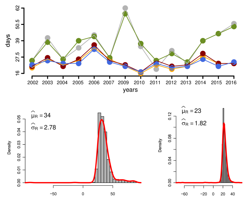
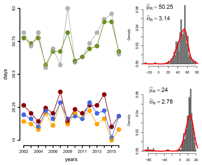
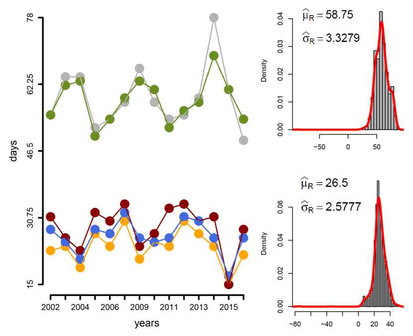
In addition to getting the optimal lag between daily precipitation and NDVI by year, via (3)-(5), we calculated the $p$-value associated to the null hypothesis of no correlation between these variables at the optimal lag. We ended up with 14 annual maps of significant delay estimates which are summarized, via the median (a well-known robust statistics), and shown in Fig.1 and 1 for the ${\bf Pn}$ and $\textnormal{LASSO}^{\tt CV}_{\tt trim}$ estimators, respectively. There are marked spatial differences between these estimators. For instance, their median and (a robust) s.d. estimate are different over the Mezquital eco-region, 28 (2.57) for $\textnormal{LASSO}^{\tt CV}_{\tt trim}$ and 58 (3.65) for ${\bf Pn}$. Observe also, Fig.2, the narrow that $\textnormal{LASSO}^{\tt CV}_{\tt trim}$’s distribution is about its center which contrast with the dispersion of ${\bf Pn}$’s distribution; their time dynamics is also different.

Figure 2. Mezquital eco-region. Left: Median of $\mathsf{TDE}$s ( ) ${\bf Pn}$, ( ) ${\bf Pn}_{\tt trim}$, ( ) ${\bf Pn}_{\tt standard}$, ( ) $\textnormal{LASSO}^{{\tt CV}}$, ( ) $\textnormal{LASSO}^{\tt CV}_{\tt trim}$. Top-right: Estimated density of ${\bf Pn}$ from 2002 to 2016 . Bottom-right: Estimated density of $\textnormal{LASSO}^{\tt CV}_{\tt trim}$ from 2002 to 2016.

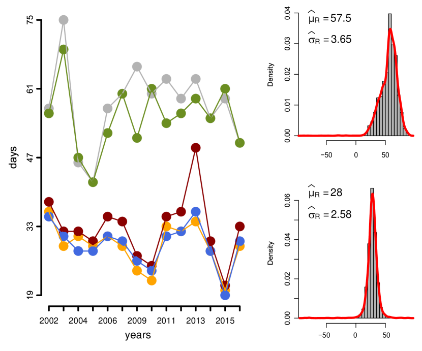
We show our analysis on Mezquital eco-region only but the differences between unscaled and trimmed $\mathsf{TDE}$s were found also in the other three eco-regions, see Supplementary Materials 7.

5. Conclusion

By incorporating sparsity we introduced a simple method to estimate the time delay between precipitation and NDVI satellite imagery time series aiming to reduce the variance of the canonical Pearson-based estimator. We showed that this goal was achieved first in simulations (and varying $\mathsf{SNR}$) and then in applications (across regions with different ecological characteristics). In practice, besides its variance reduction, the decision of (perhaps) favor the LASSO-based estimators over the canonical one should be weighted with prior information (more biophysical variables) on the characteristics of the region of interest; the interaction of more variables to describe time relationships requires further investigation.

6. Acknowledgements

The author would like to thank Rene Colditz with the Climate Action at the European Commission for introducing him to the topic of time relationships. This paper benefited also from helpful discussions with Carlos Troche, Isabel Cruz and Gabriela Villamil at CONABIO and Irina Gaynanova (Department of Statistics, Texas A&M University) and Michael Grabchak (Department of Mathematics and Statistics, UNC Charlotte).

7. Supplementary Materials

$\mathsf{TDE}$s	$\tau=37$				$\tau=110$				$\tau=183$
	Exp($\lambda$) errors				Exp($\lambda$) errors				Exp($\lambda$) errors
	$\lambda=0.125$	$\lambda=0.5$	$\lambda=2.5$		$\lambda=0.125$	$\lambda=0.5$	$\lambda=2.5$		$\lambda=0.125$	$\lambda=0.5$	$\lambda=2.5$
Madrense
${\bf Pn}$	0.001	0.286	14.754		0.001	0.101	5.495		0.000	0.002	0.063
${\bf Pn}_{\tt trim}$	0.000	106.998	360.854		0.000	0.023	1.782		0.000	0.008	346.795
${\bf Pn}_{\tt standard}$	0.000	0.160	31.066		0.000	0.040	1.966		0.000	0.004	0.218
$\textnormal{LASSO}^{0.1}$	0.000	0.121	14.610		0.000	0.039	5.182		0.000	0.004	0.062
$\textnormal{LASSO}_{\tt trim}^{0.1}$	0.000	0.036	1398.367		0.000	0.013	1.384		0.000	0.008	0.780
$\textnormal{LASSO}^{{\tt CV}}$	0.000	0.257	13.349		0.001	0.101	4.999		0.000	0.002	0.078
$\textnormal{LASSO}^{\tt CV}_{\tt trim}$	0.000	35.684	224.517		0.000	0.013	1.148		0.000	0.007	0.684
Mezquital
${\bf Pn}$	0.000	0.047	13.025		0.003	0.479	13.563		0.000	0.002	0.118
${\bf Pn}_{\tt trim}$	0.000	522.814	1265.681		0.000	0.082	6.124		0.000	0.034	126.105
${\bf Pn}_{\tt standard}$	0.000	0.043	290.854		0.000	0.114	6.420		0.000	0.009	0.571
$\textnormal{LASSO}^{0.1}$	0.000	0.051	12.970		0.000	0.089	13.101		0.000	0.006	0.120
$\textnormal{LASSO}_{\tt trim}^{0.1}$	0.000	0.051	3292.637		0.000	0.057	4.129		0.000	0.031	1.289
$\textnormal{LASSO}^{{\tt CV}}$	0.000	0.043	8.383		0.003	0.443	11.348		0.000	0.003	0.125
$\textnormal{LASSO}^{\tt CV}_{\tt trim}$	0.000	59.239	984.263		0.000	0.051	2.820		0.000	0.027	1.209
Interior Plains
${\bf Pn}$	0.000	0.140	27.744		0.001	0.492	16.470		0.000	0.008	0.821
${\bf Pn}_{\tt trim}$	0.000	831.560	2134.619		0.000	0.176	372.674		0.001	0.185	1001.198
${\bf Pn}_{\tt standard}$	0.000	0.076	624.842		0.000	0.099	7.313		0.001	0.030	3.476
$\textnormal{LASSO}^{0.1}$	0.000	0.057	25.079		0.000	0.092	16.156		0.001	0.021	0.769
$\textnormal{LASSO}_{\tt trim}^{0.1}$	0.000	0.122	4324.318		0.000	0.137	271.041		0.001	0.124	98.804
$\textnormal{LASSO}^{{\tt CV}}$	0.000	0.126	23.340		0.000	0.458	12.482		0.000	0.011	0.806
$\textnormal{LASSO}^{\tt CV}_{\tt trim}$	0.000	83.054	1617.145		0.000	0.128	6.464		0.001	0.122	52.359
Plateau Plains
${\bf Pn}$	0.000	0.445	21.739		0.001	0.302	14.249		0.000	0.004	0.981
${\bf Pn}_{\tt trim}$	0.000	558.475	1273.985		0.000	0.078	9.115		0.000	0.090	40.032
${\bf Pn}_{\tt standard}$	0.000	0.061	438.903		0.000	0.082	8.661		0.000	0.044	2.211
$\textnormal{LASSO}^{0.1}$	0.000	0.057	21.171		0.000	0.090	14.565		0.000	0.009	0.957
$\textnormal{LASSO}_{\tt trim}^{0.1}$	0.000	0.075	3644.262		0.000	0.053	36.607		0.000	0.071	3.061
$\textnormal{LASSO}^{{\tt CV}}$	0.000	0.439	19.910		0.001	0.257	12.025		0.000	0.004	0.958
$\textnormal{LASSO}^{\tt CV}_{\tt trim}$	0.000	47.604	1080.126		0.000	0.052	36.040		0.000	0.070	2.799

Table 2. Mean squared error corresponding to estimates shown in Table 1. 

Figure 3. Madrense eco-region. Left: Median of $\mathsf{TDE}$s ( ) ${\bf Pn}$, ( ) ${\bf Pn}_{\tt trim}$, ( ) ${\bf Pn}_{\tt standard}$, ( ) $\textnormal{LASSO}^{{\tt CV}}$, ( ) $\textnormal{LASSO}^{\tt CV}_{\tt trim}$. Top-right: Estimated density of ${\bf Pn}$ from 2002 to 2016 . Bottom-right: Estimated density of $\textnormal{LASSO}^{\tt CV}_{\tt trim}$ from 2002 to 2016.

Figure 4. Interior Plains eco-region. Left: Median of $\mathsf{TDE}$s ( ) ${\bf Pn}$, ( ) ${\bf Pn}_{\tt trim}$, ( ) ${\bf Pn}_{\tt standard}$, ( ) $\textnormal{LASSO}^{{\tt CV}}$, ( ) $\textnormal{LASSO}^{\tt CV}_{\tt trim}$. Top-right: Estimated density of ${\bf Pn}$ from 2002 to 2016 . Bottom-right: Estimated density of $\textnormal{LASSO}^{\tt CV}_{\tt trim}$ from 2002 to 2016.

Figure 5. Plateau Plains eco-region. Left: Median of $\mathsf{TDE}$s ( ) ${\bf Pn}$, ( ) ${\bf Pn}_{\tt trim}$, ( ) ${\bf Pn}_{\tt standard}$, ( ) $\textnormal{LASSO}^{{\tt CV}}$, ( ) $\textnormal{LASSO}^{\tt CV}_{\tt trim}$. Top-right: Estimated density of ${\bf Pn}$ from 2002 to 2016 . Bottom-right: Estimated density of $\textnormal{LASSO}^{\tt CV}_{\tt trim}$ from 2002 to 2016.

References

- Barbosa et al., (2015) Barbosa, H., Kumar, T. L., and Silva, L. (2015). Recent trends in vegetation dynamics in the south america and their relationship to rainfall. Natural Hazards, 77(2):883–899.
- Benesty et al., (2004) Benesty, J., Chen, J., and Huang, Y. (2004). Time-delay estimation via linear interpolation and cross correlation. IEEE Transactions on Speech and Audio Processing, 12(5):509–519.
- Carter, (1981) Carter, G. (1981). Time delay estimation for passive sonar signal processing. IEEE Transactions on Acoustics, Speech, and Signal Processing, 29(3):463–470.
- Colditz et al., (2017) Colditz, R. R., Villanueva, V. L. A., Tecuapetla-Gómez, I., and Mendoza, L. G. (2017). Temporal relationships between daily precipitation and NDVI time series in Mexico. In 2017 9th International Workshop on the Analysis of Multitemporal Remote Sensing Images (MultiTemp), pages 1–4.
- CONABIO, (2008) CONABIO (2008). Capital natural de México, vol. I : Conocimiento actual de la biodiversidad. Comisión Nacional para el Conocimiento y Uso de la Biodiversidad, México.
- Efron et al., (2004) Efron, B., Hastie, T., Johnstone, I., Tibshirani, R., et al. (2004). Least angle regression. The Annals of statistics, 32(2):407–499.
- Funk et al., (2015) Funk, C., Peterson, P., Landsfeld, M., Pedreros, D., Verdin, J., Shukla, S., Husak, G., Rowland, J., Harrison, L., Hoell, A., et al. (2015). The climate hazards infrared precipitation with stations — a new environmental record for monitoring extremes. Scientific Data, 2:150066.
- Hamon and Hannan, (1974) Hamon, B. and Hannan, E. (1974). Spectral estimation of time delay for dispersive and non-dispersive systems. J. R. Statist. Soc: Ser. C (Appl. Statist.), pages 134–142.
- Hannan and Thomson, (1988) Hannan, E. and Thomson, P. (1988). Time delay estimation. Journal of Time Series Analysis, 9(1):21–33.
- INEGI-CONABIO-INE, (2007) INEGI-CONABIO-INE (2007). Ecorregiones terrestres de México 2EP. Catálogo de metadatos geográficos. Comisión Nacional para el Conocimiento y Uso de la Biodiversidad, http://www.conabio.gob.mx/informacion/gis/.
- Knapp and Carter, (1976) Knapp, C. and Carter, C. (1976). The generalized correlation method for estimation of time delay. IEEE Transactions on Acoustics, Speech, and Signal Processing, 24(4):320–327.
- Schaaf and Wang, (2015) Schaaf, C. and Wang, Z. (2015). MCD43C4 MODIS/Terra+Aqua BRDF/Albedo Nadir BRDF-Adjusted Ref Daily L3 Global 0.05Deg CMG V006. Distributed by NASA EOSDIS Land Processes DAAC, https://doi.org/10.5067/MODIS/MCD43C4.006.
- Tibshirani, (2011) Tibshirani, R. (2011). Regression shrinkage and selection via the lasso: a retrospective. Journal of the Royal Statistical Society: Series B (Statistical Methodology), 73(3):273–282.
- Vicente-Serrano et al., (2013) Vicente-Serrano, S. M., Gouveia, C., Camarero, J. J., Beguería, S., Trigo, R., López-Moreno, J. I., Azorín-Molina, C., Pasho, E., Lorenzo-Lacruz, J., Revuelto, J., et al. (2013). Response of vegetation to drought time-scales across global land biomes. Proceedings of the National Academy of Sciences, 110(1):52–57.