Atomistic structure learning

Abstract

One endeavour of modern physical chemistry is to use bottom-up approaches to design materials and drugs with desired properties. Here we introduce an atomistic structure learning algorithm (ASLA) that utilizes a convolutional neural network to build 2D compounds and layered structures atom by atom. The algorithm takes no prior data or knowledge on atomic interactions but inquires a first-principles quantum mechanical program for physical properties. Using reinforcement learning, the algorithm accumulates knowledge of chemical compound space for a given number and type of atoms and stores this in the neural network, ultimately learning the blueprint for the optimal structural arrangement of the atoms for a given target property. ASLA is demonstrated to work on diverse problems, including grain boundaries in graphene sheets, organic compound formation and a surface oxide structure. This approach to structure prediction is a first step toward direct manipulation of atoms with artificially intelligent first principles computer codes.

The discovery of new materials for energy capture and energy storage and the design of new drugs with targeted pharmacological properties stand out as the ultimate goals of contemporary chemistry research and materials science Schneider and Fechner (2005); Tabor et al. (2018). The design spaces for these problems are immense Kirkpatrick and Ellis (2004) and do not lend themselves to brute force or random sampling McNally et al. (2011). This has led to the introduction of screening strategies in which computational chemistry is utilized to identify the more promising candidates before experimental synthesis and characterization is carried out Greeley et al. (2006). Machine learning techniques have further been introduced to speed up such screening approaches Gómez-Bombarelli et al. (2016). Unsupervised machine learning may serve to categorize substances whereby further search efforts can be focused on representative members of different categories Duan et al. (2010). Supervised machine learning may direct the searches even further as properties of unknown materials are predicted based on the properties of known materials Pilania et al. (2013). In recent years, there has been a move toward even more powerful use of machine learning, namely the employment of active learning schemes such as reinforcement learning Olivecrona et al. (2017); Popova et al. (2018).

In active learning, the computational search is self-directed. It thereby becomes independent on both the availability of large datasets as in big data approaches Saal et al. (2013) and on the formulation by the research team of a valid guiding hypothesis. In the chemistry domain, the power of active learning has been demonstrated in drug design. Schemes in which molecules may be built from encoding strings, e.g. the simplified molecular-input line-entry system (SMILES) strings, have led to artificial intelligence driven protocols, where a neural network based on experience spells the string for the most promising next drug to be tested Gómez-Bombarelli et al. (2018). For instance, generative adversarial networks (GANs) have been utilized for this Putin et al. (2018).

The strength of reinforcement learning was recently demonstrated by Google DeepMind in a domain accessible to the general public Mnih et al. (2015); Silver et al. (2016, 2017). Here Atari 2600 computer games and classical board games such as Chess and Go were tackled with techniques from computer vision and image recognition and performances were achieved that surpassed those of all previous algorithms and human champions.

Figure 1: The three phases of structure search in ASLA. In each step $t$ of the building phase for episode $i$, the atomistic structure $s^{(i)}_{t}$ is input to the CNN that outputs $Q$-values (blue raster plot) estimating the expected reward for the final structure, $s^{(i)}_{\mathrm{final}}$. $N$ consecutive actions, $a^{(i)}_{t}$, are taken according to an $\varepsilon$-greedy policy thereby building the final structure. In the evaluation phase, a structure property, $\mathcal{P}^{(i)}$, is calculated. All episode steps are stored in the replay buffer from which a training batch is extracted. Properties contained in the batch are then converted to rewards which represent $Q_{\mathrm{target}}$-values that the CNN is trained toward predicting.

I Atomistic reinforcement learning

In the present work, we aim at bringing the image recognition approach into the domain of quantum chemical guided materials search. I.e. we formulate a protocol for deep reinforcement learning in which a convolutional neural network (CNN) starts with zero knowledge and builds up its knowledge of optimal organisation of matter via self-guided recurring inquiries for its produced candidate structures. By optimal organisation of matter, we consider in this first application primarily the thermodynamical stability of a configuration as revealed by a quantum mechanical simulation. The network is fed a real-space image-like representation of the chemical structures and is trained by ”playing” against itself, striving to beat the properties of its ever best candidate. As a result, the blueprint for favourable atomic arrangements is directly searched for and learned by the network. This deviates from existing approaches that based on intricate descriptors of the atomic environments Huang and von Lilienfeld (2016); Faber et al. (2017) attempt to facilitate the calculation of quantum mechanical energy landscapes at a low cost Bartók et al. (2010); Behler and Parrinello (2007); Rupp et al. (2012); Li et al. (2015); Smith et al. (2017); Chmiela et al. (2017) and use them in traditional global structure optimisation methods Ouyang et al. (2015); Huang et al. (2018); Kolsbjerg et al. (2018). Technical details on our CNN architecture and training procedure are described in Methods.

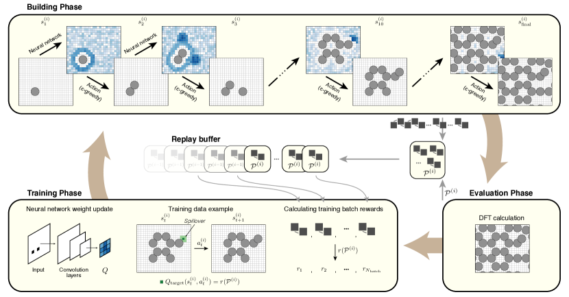
The goal of an ASLA structure search is to generate structures of a given stoichiometry which optimise a target structural property, $\mathcal{P}$. This is done by repeatedly generating candidate structures, evaluating a reward according to $\mathcal{P}$, and learning from these experiences, or episodes, how to generate the globally optimal structure. The three phases of an ASLA structure search, building, evaluation and training, are depicted in Fig. 1.

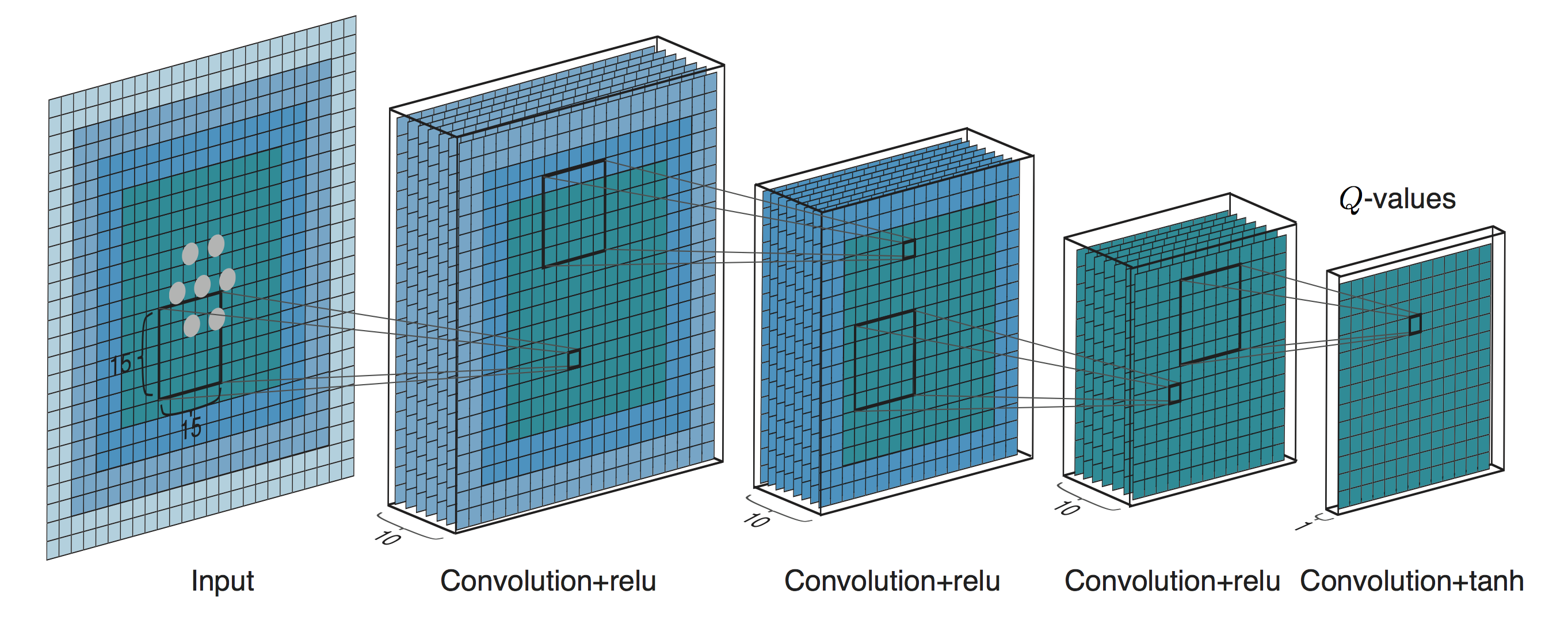
In the building phase, atoms are placed one at a time on a real space grid to form a structure candidate. $N$ atoms are placed in a sequence of actions $a_{t}\in\{a_{1},a_{2},...,a_{N}\}$. At each step of the candidate generation ASLA attempts to predict the expected reward of the final structure given the incomplete current structure. This information is stored in a CNN, which takes as input the incomplete, current configuration $s_{t}$, encoded in a simple one-hot tensor, and outputs the expected reward ($Q$-value) for each available action (see Extended Data Fig. 1). The action is chosen either as the one with the highest $Q$-value (greedy), or in $\varepsilon$-fraction of the time at random to encourage exploration. After the completion of a structure (episode $i$), the property $\mathcal{P}^{(i)}$ of that final structure $s^{(i)}_{\mathrm{final}}$ is calculated in the evaluation phase, e.g. as the potential energy according to density functional theory (DFT), $\mathcal{P}^{(i)}=E_{\mathrm{DFT}}(s^{(i)}_{\mathrm{final}})$, in which case ASLA will eventually identify the thermodynamically most stable structure at $T=0$ K.

In the training phase, the CNN parameters are updated via backpropagation, which lowers the root mean square error between predicted $Q$-values and $Q_{\mathrm{target}}$-values calculated according to:

$$Q_{\mathrm{target}}(s_{t}^{(i)},a_{t}^{(i)})=r(\mathcal{P}^{(i)}),$$ (1)

where $r\in\left[-1,1\right]$ is the reward of completing episode $i$ with property $\mathcal{P}^{(i)}$, where $1$ is considered the better reward (reflecting e.g. the lowest potential energy). Thus, the $Q$-value of action $a_{t}^{(i)}$ of step $t$ is converged toward the reward following the properties of the final configuration $s_{\mathrm{final}}^{(i)}$, an approach also taken in Monte Carlo reinforcement learning Sutton and Barto (2018). Equation 1 ensures that actions leading to desired structures will be chosen more often. A training batch of $N_{\mathrm{batch}}$ state-action-property tuples, $(s_{t}^{(i)},a_{t}^{(i)},\mathcal{P}^{(i)})$, is selected from the most recent episode, the best episode, and via experience replay Mnih et al. (2015) of older episode steps. The batch is augmented by rotation of structures on the grid. Rotational equivariance is thus learned by the CNN instead of encoded in a molecular descriptor as is done traditionally Rupp et al. (2012); Huang and von Lilienfeld (2016); Schütt et al. (2017); Faber et al. (2017). This allows the CNN to learn and operate directly on real space coordinates. We furthermore take advantage of the smoothness of the potential energy surface by smearing out the learning of $Q$-values to nearby grid points (spillover). See Methods for details.

Figure 2: ASLA learns to build a sheet of graphene. a, One example of predicted $Q$-values for $t=1$, $10$ and $20$ after 0, 200, 1000 and 2000 episodes respectively. b, An example of an agent which builds the globally optimal structure in a different sequence.

II Building graphene

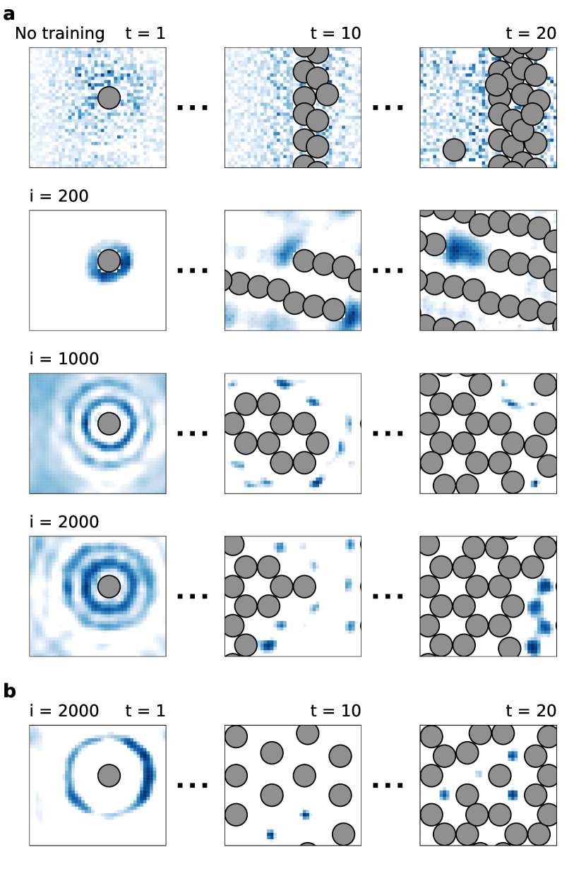
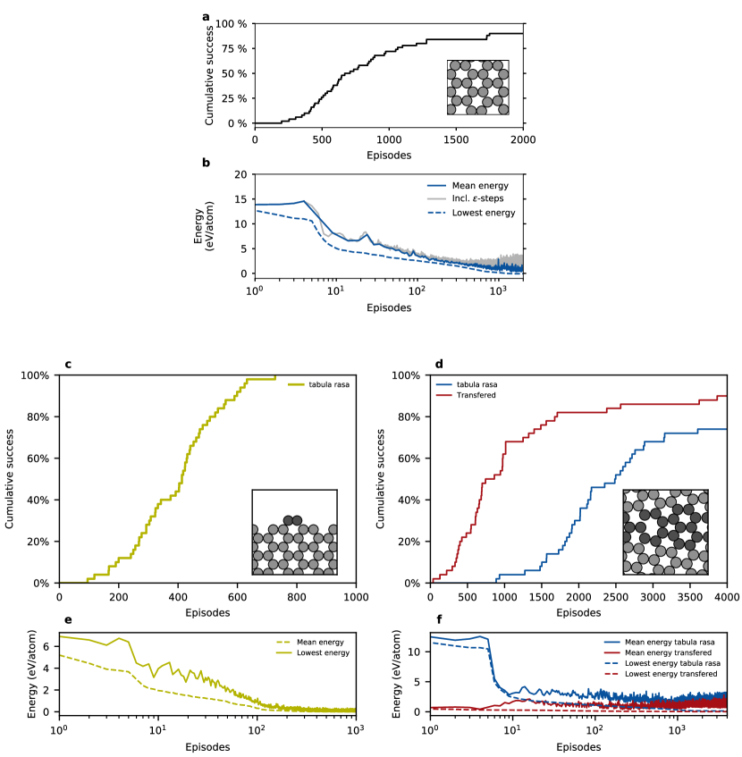
As a first demonstration, an instance of ASLA (an agent) learns how to build a sheet of pristine graphene. One carbon atom is present in an initial template structure, $s_{1}$, and $N=23$ carbon atoms are placed by the agent on a grid with periodic boundary conditions. Figure 2a presents one example of predicted $Q$-values for $t=1,10,20$ during the building phase of one agent (for statistics involving 50 independent agents, see Extended Data Fig. 2a+b). Values are shown for the tabula rasa agent (the untrained agent) and for the agent trained for 200, 1000 and 2000 episodes. At first, the untrained CNN outputs random $Q$-values stemming from the random initialization, and consequently a rather messy structure is built. After 200 episodes, the agent has found the suboptimal strategy of placing all the carbon atoms with reasonable interatomic distances, but more or less on a straight line. The angular preference at this point is thus to align all bonds. After 1000 episodes, the agent has realized that bond directions must alternate and now arrives at building the honeycomb pattern of graphene. After 2000 episodes, the agent still builds graphene, now in a slightly different sequence.

The evolution over the episodes of the overall ring-shaped patterns in the $Q$-values for $t=1$ show how the agent becomes aware of the correct interatomic distances. The barely discernible six-fold rotational symmetric modulation of the $Q$-values that develop within the rings ends up being responsible for the agent choosing bond directions that are compatible with accommodating graphene within the given periodic boundary conditions.

Interestingly, the agent may discover the optimal structure through different paths due to the random initialization and the stochastic elements of the search. In Fig. 2b, another agent has evolved into building the graphene structure in a different sequence. This time the agent has learned to first place all next-nearest atoms (half of the structure) in a simple, regular pattern. The remaining atoms can then be placed in the same pattern but shifted. One can imagine how this pattern is easily encoded in the CNN.

III Transfer learning

Figure 3: Demonstration of transfer learning. CPU hours required to solve the graphene grain boundary problem without and with transfer learning (left and right part, respectively). The transferred agents pay a small amount of computational resources on the cheap graphene edge problem to get a head start on the grain boundary problem, where they solve it 50% of the time using 57.2 CPU hours or less. However, the tabula rasa agents need 143.0 CPU hours to achieve the same.

Figure 4: $Q$-values (left) and relevance values (right) given by an agent trained on the graphene edge. a, The agent has learned that closing a six-membered carbon ring results in low potential energy and assigns high $Q$-values for these positions. b, Relevance values for the action ($\times$) reveal that nearby atoms are responsible for the high $Q$-values. c, If an atom is too close to an action ($\times$), this atom is responsible for low $Q$-values. d, The agent recognizes similar arrangements of atoms in the grain boundary (after 3 atoms have been added) and assigns high $Q$-values for corresponding actions. e and f, Although the agent has never seen this configuration, it applies the local knowledge learned in the graphene edge problem.

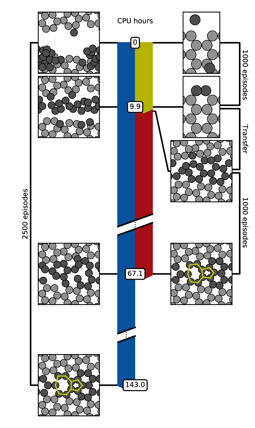
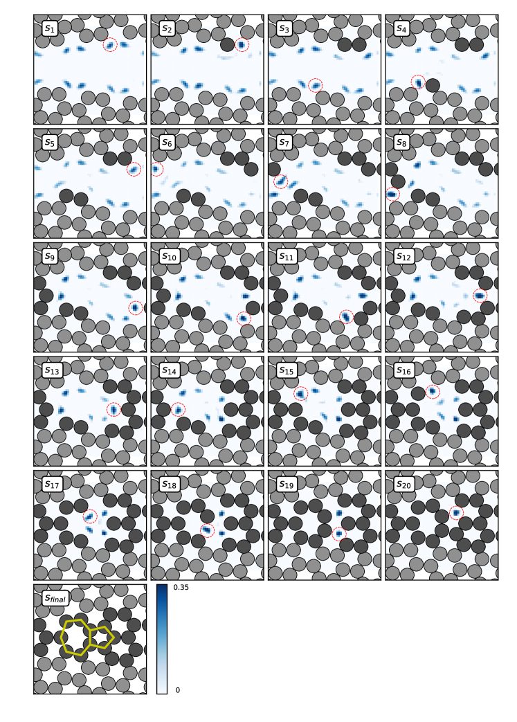
Moving on to a more complex problem, we consider a graphene grain boundary which has been studied by Zhang et al. Zhang et al. (2015). Here, an ASLA agent must place 20 atoms in between two graphene sheets that are misaligned by 13.17^∘, which induces a pentagon-heptagon (5-7) defect in the grain boundary. The complete structure under consideration is comprised of 80 atoms per cell. We first run an ensemble of 50 tabula rasa agents. Within $\sim$2500 episodes, half of the agents have found the 5-7 defect structure as the optimal structure (Fig. 3 and Extended Data Fig. 2d).

Figure 5: Building C₃H₄O₂ compounds. a, Predicted $Q$-values in the process of building ethylene + carbon dioxide. b, Distribution of molecular compounds of stoichiometry C₃H₄O₂, sorted by formation energy, as found by 25 agents during 10000 episodes. For all structures see Extended Data Fig. 6. The sum exceeds 100% as a punishing term is employed once a build has been found repeatedly (see Methods). c, Search results when rewarding O binding to 2$\times$C, coding for ether and epoxy groups. d, Search results when rewarding C binding to C and 2$\times$O, coding for epoxy and acidic groups. e, Search results when rewarding C binding to O and 2$\times$C, coding mainly for cyclic C₃ groups.

The number of required episodes can be lowered significantly with the use of transfer learning. Transfer learning is a widely used approach in many domains where knowledge is acquired for one problem and applied to another Pan and Yang (2010); Taylor and Stone (2009). Our CNN architecture allows us to utilize transfer learning, since each $Q$-value is evaluated based on the atomic-centered environment, which is independent of the cell size. The CNN may learn elements of how to discriminate favourable and unfavourable atomic arrangements in simple systems, and retain this knowledge when used in larger, more computationally expensive systems. To demonstrate this, we choose a simpler problem, namely that of placing two atoms at the edge of a graphene nanoribbon (see upper right corner of Fig. 3). Using our DFT setup this simple problem is cheaper to compute by a factor of $\sim$5 due to the smaller number of atoms. The agents trained on this problem are transferred to build the grain boundary. Although the graphene edge problem is too simple to immediately infer the full solution to the grain boundary problem (Extended Data Figs. 3+4), the pretrained agents hold a clear advantage over the tabula rasa agents. The average energies during the search reveal that the transferred agents produce structures close in energy to the globally optimal structure even before further training (Extended Data Fig. 2f), and now only about 1000 episodes are required for half of the agents to find the 5-7 defect.

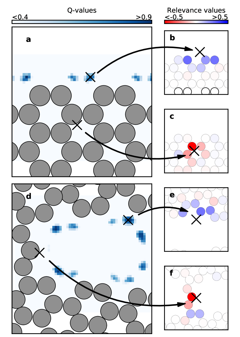
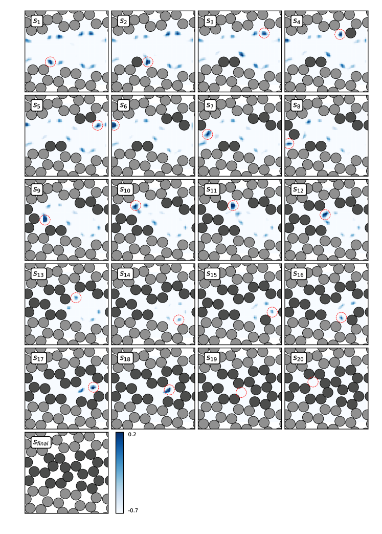
To inspect the agents’ motivation for predicting given $Q$-values, we employ a variant of the layer-wise relevance propagation method (see Methods). The relevance value of an atom indicates how influential that atom was in the prediction of the $Q$-value, where 1 is positive influence, $-1$ is negative influence and $0$ is no influence. We show the $Q$- and relevance values for the graphene edge and grain boundary problems in Fig. 4, as given by one of the agents that has only been trained on the graphene edge problem. In addition to solving the graphene edge problem by closing a six-membered ring, the agent recognizes similar local motifs (unclosed rings) in the grain boundary problem which lead to favourable actions even without further training (Fig. 4b+e). The relevance values in Fig. 4c+f also reveal that the agent has learned not to place atoms too close no matter the local environment.

IV Molecular design

The ability of ASLA to build multicomponent structures is easily accommodated by adding to the CNN input a dimension representing the atomic type. The CNN will then correspondingly output a map of $Q$-values for each atomic type. When building a structure, a greedy action now becomes that of choosing the next atom placement according to the highest $Q$-value across all atomic types.

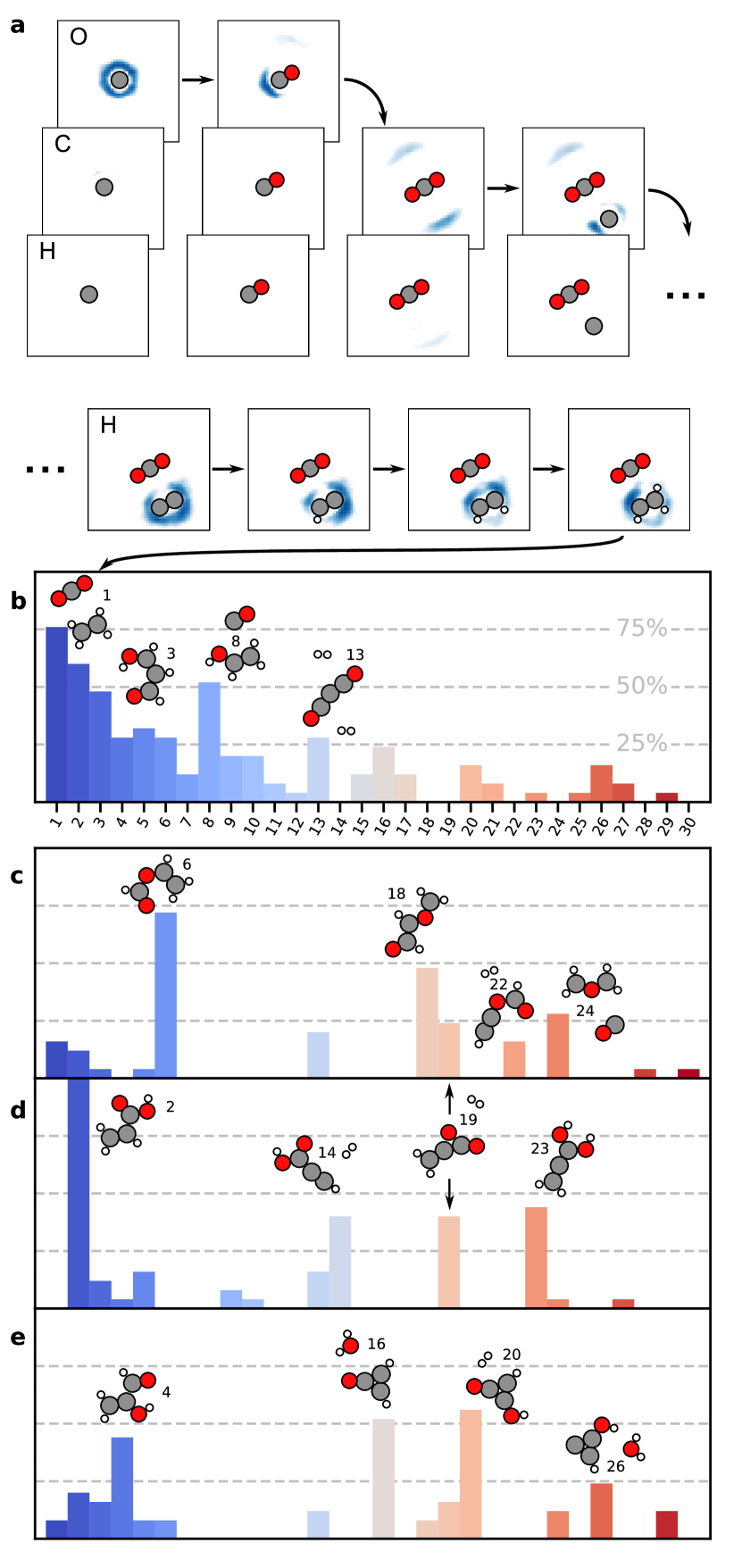
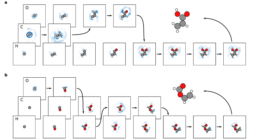
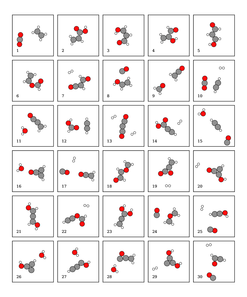
Figure 5a illustrates the building strategy of a self-trained ASLA agent assembling three carbon, four hydrogen and two oxygen atoms into one or more molecules. The agent identifies the combination of a carbon dioxide and an ethylene molecule as its preferred building motif. The reason for this build is the thermodynamic preference for these molecules with the chosen computational approach. Depending on the initial conditions and the stochastic elements of ASLA, we find that other agents may train themselves into transiently building a plethora of other chemically meaningful molecules given the present 2D constraint. The list of molecules built includes acrylic acid, vinyl formate, vinyl alcohol, formaldehyde, formic acid and many other well known chemicals (see Extended Data Figs. 5+6).

Figure 5b reveals the distribution of molecules built when 25 independent agents are run for 10000 episodes, and shows that ASLAs prolific production of different molecules has a strong preference for the thermodynamically most stable compounds (blue bars). This is in accordance with the reward function depending solely on the stability of the molecules. We find, however, that the building preference of ASLA may easily be nudged in particular directions exploiting the bottom-up approach taken by the method. To do this we modify the property function slightly (see Methods) rewarding structures that contain some atomic motif. The histogram in Fig. 5c shows the frequencies with which molecules are built once the reward is increased for structures that have an oxygen atom binding to two carbon atoms. No constraints on the precise bond lengths and angles are imposed, and ASLA consequently produces both ethers (structures 6, 18, 22 and 24) and an epoxy molecule (structure 19) at high abundance, while the building of other molecules is suppressed.

The production of the epoxy species intensifies as evidenced by Fig. 5d once the rewarding motif becomes that of a carbon atom bound to one carbon and two oxygen atoms. This motif further codes very strongly for acidic molecules (structures 2, 14 and 23). In fact, now every agent started eventually ends up building acrylic acid (structure 2) within the allowed number of episodes.

Figure 6: Learning to build a Ag₁₂O₆ overlayer structure. a, Scanning tunneling microscopy image of the Ag(111)-p(4 $\times$ 4)-O phase (adapted from Schnadt et al. (2006)). b, Experimental information on super cell, absence of atoms in corner regions and stoichiometry is used as input to ASLA. c, Transfer of ASLAs 2D structure to become a surface layer in a DFT slab calculation. d, Predicted $Q$-values for an episode where the agent has self-learned to build the globally optimal overlayer structure.

Switching to a rewarding motif consisting of a carbon atom binding to one oxygen and two carbon atoms we find the results of Fig. 5e. Now, the search builds almost twice as many 2-hydroxyacrylaldehyde molecules (structure 4) and adopts a clear preference for molecules with three carbon atoms in a ring, such as the aromatic cyclopropenone and related molecules (structures 16, 20 and 26).

The ability of ASLA to direct its search in response to variations in the reward function represents a simple illustration of how automated structure search may lead to design of molecules with certain properties. The present approach may be used in search for larger organic compounds with some given backbone building blocks or some assemblies of functional groups. It might also be directly applicable when searching for organo-metalic compounds where the malleable bonds mean that the desired motif may only be specified loosely as done here. However, for searches that target e.g. ionization potentials, HOMO-LUMO gaps, deprotonation energies, and other global properties of molecules, we envisage that more elaborate strategies for directing the searches must be implemented in order to truly conduct molecular design.

V Surface oxide on Ag(111)

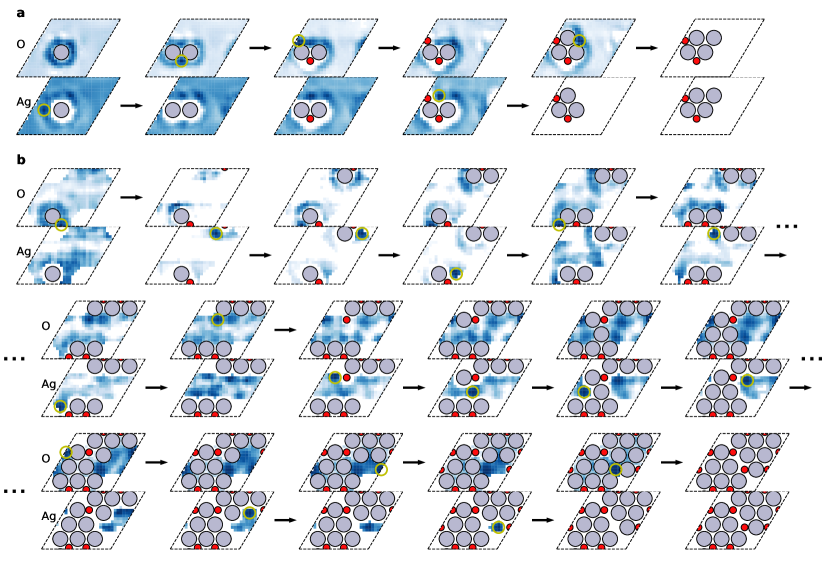
As a final, non-trivial example, the structure of oxidized silver, known to be an efficient catalyst for e.g. epoxidation reactions Michaelides et al. (2005), is considered. For this system, one particular surface oxide phase, Ag(111)-$p(4\times 4)$-O, has been subject to many studies since the 1970s resulting in several proposed structures Michaelides et al. (2005); Rovida et al. (1974); Carlisle et al. (2000); Schnadt et al. (2006); Schmid et al. (2006). Key experimental observations include STM images Carlisle et al. (2000); Schnadt et al. (2006); Schmid et al. (2006) (Fig. 6a) of a regular rhombic surface unit cell containing 12 Ag atoms and 6 O atoms per unit cell with void regions amounting to approximately 25% of the cell Schmid et al. (2006). Using this information, we prepare a grid (Fig. 6b) on which an agent can build a Ag₁₂O₆ overlayer structure. The property of a specific build is the DFT potential energy of the overlayer structure once placed on a single, fixed Ag(111) layer representing the silver crystal (Fig. 6c). Employing transfer learning, starting from an agent trained in forming Ag₄O₂ clusters (Extended Data Fig. 7) ASLA proves capable of learning by itself to build the intricate structure shown in Fig. 6d. In hindsight, this structure might appear highly intuitive to a trained inorganic surface chemist, yet despite many efforts Michaelides et al. (2005) this correct structure remained elusive for more than half a decade after the first characterization by STM imaging in 2000 until it was finally identified in 2006 Schnadt et al. (2006); Schmid et al. (2006). It is intriguing how such a puzzling structure may now emerge from a fully autonomous reinforcement learning setup and a CNN of a relatively modest size.

VI Outlook

In the present work, we have demonstrated how deep reinforcement learning can be used in conjunction with first principles computational methods to automate the prediction of 2D molecular and inorganic compounds of optimal stability. The work is readily generalized into handling 3D atomistic structures by turning to 3D convolution kernels and adding one more spatial dimension to the input grid and to the output $Q$-value tensor. This will increase the computation load of each $Q$-value prediction linearly in the number of grid points added in the 3rd dimension, which is manageable. It will, however, also open for more complex problems to be addressed which will require more episodes to converge.

As more complex 2D or even 3D problems are tackled with the method, we foresee the need for introducing further means of directing the global optimisation. The reinforcement protocol will be slow in detecting structures that require several favourable $\varepsilon$-moves to form and will suffer from conservatism, exploring mainly close to previously built structures. Here, adding e.g. a beam search strategy, Monte Carlo tree search and possibly combining the method with a property predictor network allowing for the screening of several orders of magnitude more structures than those handled with the first principles method may be viable strategies.

Finally, we note that agents trained to act on a variable number of atoms are desirable as they will be more versatile and capable of solving more diverse problems. Such agents may be obtained by introducing chemical potentials of atomic species. Notwithstanding such possible extensions, we consider the present work to represent a first peek into a rich research direction that will eventually bring about first principles computer codes for intelligent, bottom-up design and direct manipulation of atoms in chemical physics and materials science.

Acknowledgements We acknowledge support from VILLUM FONDEN (Investigator grant, project no. 16562).

Author contributions All authors contributed to conceiving the project, formulating the algorithms and writing the computer codes. KHS acted as scrum master. MSJ, ELK and TLJ established the first proof-of-concept implementation. MSJ conducted the pristine graphene calculations. HLM did the transfer/layer-wise relevance propagation calculations. SAM did the multi-component/design calculations, while BH did the AgO calculations. MSJ, HLM, SAM and BH wrote the paper.

VII Methods

Neural network architecture. In all presented applications, a plain CNN with three hidden layers of each ten filters implemented with Tensorflow Abadi et al. (2015) is used (see Extended Data Fig. 1). The number of weights in the network depends on the filter size, grid spacing and number of atomic species, but is independent on the computational cell size used and on the number of actions taken. Hidden layers are activated with leakyRELU functions, while the output is activated with a tanh function to get $Q\in[-1,1]$. The input is a one-hot encoded grid (1 at atom positions, 0 elsewhere), and the correct number of output $Q$-values (one per input grid point) is retained by adding padding to the input, with appropriate size and boundary conditions. Other layer types, such as a fully connected layer, would disrupt the spatial coherence between input and output and are thus not used. The filter dimensions depend on a user-chosen physical radius and the grid spacing. E.g. a filter of width 3 Å on a grid with spacing 0.2 Å has $15\times 15$ weights per convolution kernel.

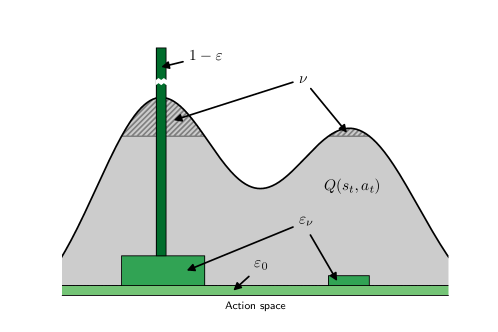
Search policy. An action is chosen with a modified $\varepsilon$-greedy sampling of the $Q$-values (see Extended Data Fig. 8). The highest $Q$-value is chosen with $(1-\varepsilon)$ probability, and a pseudo-random $Q$-value is chosen with $\varepsilon=\varepsilon_{0}+\varepsilon_{\nu}$ probability, where $\varepsilon\in\left[0,1\right]$. Two types of actions contribute to $\varepsilon$. There is an $\varepsilon_{0}$ probability that the action is chosen completely randomly, while the actions are chosen among a fraction $\nu$ of the best $Q$-values with $\varepsilon_{\nu}$ probability (hence a pseudo-random action), where $\nu\in\left[0,1\right]$. The selectivity parameter $\nu$ is introduced to avoid excessive exploration of actions estimated to result in low-reward structures. To ensure that greedy policy builds are included in the training, every $N_{p}=5$th episode is performed without $\varepsilon$-actions. Atoms cannot be placed within some minimum distance of other atoms (defined as a factor $c_{1}$ times the average of the involved covalent radii). This is to avoid numerical complications with the use of DFT implementations. A maximum distance, with factor $c_{2}$, is used for the C₃H₄O₂ system to avoid excessive placement of isolated atoms (Fig. 5, $c_{2}=2.5$).

Neural network training. In all results of the present work, the training batch contains $N_{\textrm{batch}}$ episode steps before augmentation. Among these are all steps building the optimal structure identified so far, and all steps building the most recent candidate structure. The remaining episodes are picked at random from the entire replay buffer. If any state-action pair appears multiple times in the replay buffer, only the episode step with the property that leads to the highest reward may be extracted.

The reward function scales all batch property values linearly to the interval $[-1,1]$, where 1 is considered the better reward. If the property values span a large interval, all values below a fixed property value is set to $-1$ in order to maintain high resolution of rewards close to 1. This is done for the graphene systems and the C₃H₄O₂ compounds, where the lower limit of $-1$ is fixed at an energy which is $\Delta E$ higher (less stable) than that of the energy corresponding to a reward of 1.

Spillover is incorporated into the backpropagation cost function by also minimizing the difference between $Q_{\mathrm{target}}$ and predicted $Q$-values of grid points within some radius $r_{\mathrm{spillover}}$ of the grid point corresponding to the action $a_{t}$. In all of the present work, $r_{\mathrm{spillover}}=0.3$ Å. The complete cost function is thus

$$J=\frac{1}{m}\sum_{i=1}^{m}\left[Q-Q_{\mathrm{target}}+\sum_{j}\eta_{j}(Q_{j}^{\mathrm{spillover}}-Q_{\mathrm{target}})\right]^{2},$$ (2)

where $m$ is the augmented batch size, and $\eta_{j}$ is a weight factor determining the amount of spillover for a grid point $j$ within the radius $r_{\mathrm{spillover}}$. Thus, the predicted $Q$-values of adjacent grid points, $Q_{j}^{\mathrm{spillover}}$, are also converged toward the $Q_{\mathrm{target}}$ value, but at a different rate determined by the factor $\eta_{j}$ ($\eta_{j}=0.1$ in the present work). CNN parameters are optimised with the ADAM gradient descent optimiser.

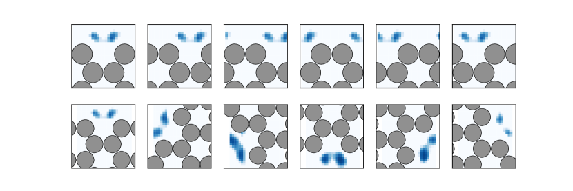
Rotational equivariance is learned from augmenting the batch by rotating produced configurations (see Extended Data Fig. 9). Similarly, to enable some spillover for AgO where the grid spacing used (0.5 Å) was larger than $r_{\mathrm{spillover}}$ we augmented the batch by ($s^{(i)}_{t}$, $\tilde{a}^{(i)}_{t}$, $\mathcal{P}^{(i)}$), where $\tilde{a}^{(i)}_{t}$ deviates from the actually tested action, $a^{(i)}_{t}$, by $\pm$ one pixel in the $x-$ and $y-$directions.

Layer-wise relevance propagation. Layer-wise relevance propagation seeks to decompose the CNN output, i.e. the $Q$-value, and distribute it onto the CNN input in a manner that assigns a higher share, or relevance, to more influential input pixels (Fig. 4). The outputs are distributed layer by layer, while conserving relevance, such that the sum of the relevance values in each layer equals the output. The relevances are computed by backwards propagating the output through the CNN. We compute the relevance of neuron $i$ in layer $l$ by

$$R_{i}^{l}=\sum_{j}\frac{x_{i}w_{ij}}{\sum_{i}x_{i}w_{ij}+\tau}R_{j}^{l+1}.$$ (3)

Here, $x_{i}$ is the activation of node $i$ connected to node $j$ by the weight $w_{ij}$, while $\tau$ is a small number to avoid numerical instability when the denominator becomes small. Equation 3 distributes relevance of neuron $j$ to neuron $i$ in the preceding layer according to the contribution to the pre-activation of neuron $j$ from neuron $i$ weighted by the total pre-activation of neuron $j$. Equation 3 implies that bias weights are not used whenever relevance values need to be calculated (i.e. in the graphene grain boundary and edge systems).

Exploration via punishment. The agent might settle in a local optimum, where a highly improbable series of $\varepsilon$-moves are needed in order to continue exploring for other optima. To nudge the agent onwards we introduce a punishment which is activated when the agent builds the same structure repeatedly, indicating that it is stuck (similar to count-based exploration strategies in reinforcement learning Xu et al. (2017)). The punishment term is added to the property value:

$$\tilde{\mathcal{P}}^{(i)}=\mathcal{P}^{(i)}+\sum_{m}A\exp\left(-\frac{|s^{(i)}_{\mathrm{final}}-s^{(m)}_{\mathrm{final}}|^{2}}{2\sigma^{2}}\right),$$ (4)

where $m$ runs over structures, $s^{(m)}_{\mathrm{final}}$, to be punished (repeated structures), and where $A$ and $\sigma$ are constants. The distance $|s^{(i)}_{\mathrm{final}}-s^{(m)}_{\mathrm{final}}|$ is evaluated using a bag-of-bonds representation Hansen et al. (2015) of the structures. Both C₃H₄O₂ and the AgO system utilize this technique.

Property function modification. To facilitate molecular design the property values are changed to

$$\mathcal{P}^{(i)}=E_{\mathrm{DFT}}(s^{(i)}_{\mathrm{final}})\cdot f(s^{(i)}_{\mathrm{final}}),\\$$ (5)

where $f$ artificially strengthens the potential energy for structures fulfilling some criterion $g$ according to:

$$f(s)=\left\{\begin{array}[]{ll}1+\lambda&\mathrm{if\ }s\mathrm{\ fullfills\ }g\\ 1&\mathrm{otherwise.}\end{array}\right.$$

For instance, $g$ may be the criterion that some oxygen atom in the structure is connected to two carbon atoms no matter the angle (two atoms are considered connected if they are within the sum of the covalent radii + 0.2 Å). In the present work, $\lambda=0.2$ is used.

DFT calculations. All calculations are carried out with the grid-based projector augmented-wave (GPAW Mortensen et al. (2005)) software package and the atomic simulation environment (ASE) Larsen et al. (2017). The Perdew-Burke-Ernzerhof (PBE) exchange-correlation functional Perdew et al. (1996) is used together with a linear combination of atomic orbitals (LCAO) for the graphene, and AgO surface reconstruction, and a finite difference method for the C₃H₄O₂ compound. All systems are modelled in vacuum. For further details on the system cell and grid dimensions, see Extended Data Table 1.

Hardware. All calculations were done on a Linux cluster with nodes having up to 36 CPU cores. Neural network and DFT calculations were parallelized over the same set of cores on one node. The CPU times given for the transfer learning problem presented in Fig. 3 were recorded when 4 CPU cores were used.

Hyperparameters. For all relevant hyperparameters, see Extended Data Table 1.

Extended Data Figure 1: Layout of the CNN architecture for one atom species. The input is atom positions mapped to a grid in a one-hot encoding with 1 at atom positions and 0 elsewhere. The input is forwarded through three convolution layers with 10 filters in each layer, arriving at the $Q$-values. We use convolution layers (i.e. no pooling, fully-connected layers, etc.) such that we can map each $Q$-value to a real space coordinate. We pad the input appropriately, taking periodic boundary conditions into account if needed. Notice that the network accepts grids of arbitrary size since the output size scales accordingly. The input can readily be expanded in the third dimension to accommodate systems of several atomic species.

Extended Data Figure 2: ASLA searches for graphene systems. a, The success of finding the structure of pristine graphene. After 2000 episodes with 50 independent ASLA agents, 90% have found the globally optimal structure (inset) within 0.05 eV per atom. b, The energy of produced structures averaged over 50 agents relative to the energy of the globally optimal structure. The decrease in energy is most significant in the first few hundred episodes, where ASLA learns to place atoms at reasonable interatomic distances. c, The success of finding the structure of the graphene edge. After $\sim$700 episodes all agents (a total of 50) find the solution within 0.05 eV per atom. d, The success of finding the graphene grain boundary within 0.15 eV per atom, with and without transfer learning. An ensemble of 50 agents are started tabula rasa, while the 50 agents from the graphene edge problem are reused for transfer.

Extended Data Figure 3: Transfered agent with no further training on the grain boundary problem. This agent has only been trained on the graphene edge problem. $Q$-values are displayed in blue, and the red dotted circle indicates the position of the highest $Q$-value. The agent recognizes the similar environment between the two problems and builds a reasonable first guess. However, it does not know the complete solution.

Extended Data Figure 4: Transfered agent with further training on the grain boundary. The same situation as in Extended Data Fig. 3, however, now the agent has been further trained on this problem for 555 episodes. The agent has learned to accommodate the 5-7 defect.

Extended Data Figure 5: Building a C₃H₄O₂ molecule. a, Example of an acrylic acid build. In contrast to the carbon dioxide + ethylene structure, all carbon atoms are now placed prior to oxygen atoms. b, A vinyl formate build. A hydrogen atom is placed to build the formate before ASLA completes the structure by attaching the vinyl group.

Extended Data Figure 6: Structures found for C₃H₄O₂. The 30 most stable structures found by the 4$\times$25 independent agents employed in Fig. 5b-e. For isomers that may appear in several conformational forms, only one conformer is depicted. The structures shown have been relaxed without the use of the grid. Structures were counted in Fig. 5b-e for greedy policy builds (every $N_{p}$’th episode) whenever (i) their graph was recognized as coinciding with those of the depicted structures, and (ii) their bond lengths and angles did not cause issues suggesting that they would not relax into the structures shown.

Extended Data Figure 7: Predicted $Q$-values for AgO structures. Examples of full builds for a, A silver surface, Ag(111), supported Ag₄O₂ cluster structure and b, The Ag₁₂O₆ overlayer structure reported in Schnadt et al. (2006); Schmid et al. (2006). The first Ag atom is placed at an fcc position with respect to the 2nd Ag layer. Other agents were trained for different choices of where the first Ag atom was placed but did not result in better structures. As in the entire work, the DFT total energy was evaluated without relaxation. The lateral separation of the two layers in the DFT calculation was chosen as 2.3 Å and any buckling within the AgO overlayer was thus neglected.

Extended Data Figure 8: Illustration of the pseudo-random $\varepsilon$-greedy policy. From the entire space of actions, the action with the highest $Q$-value is chosen with $1-\varepsilon$ probability, while a pseudo-random action is chosen with $\varepsilon=\varepsilon_{0}+\varepsilon_{\nu}$ probability. There is a probability $\varepsilon_{0}$ that it is chosen completely randomly, while the action is chosen among a fraction $\nu$ of the highest $Q$-values with $\varepsilon_{\nu}$ probability.

Extended Data Figure 9: $Q$-values in the graphene edge problem for an agent trained for 700 episodes. The top row demonstrates the translational equivariance of the $Q$-values directly inherited from the architecture of the CNN. The bottom row demonstrates the approximate rotational equivariance learned by the agent from augmenting the training data with rotated copies.

Extended Data Table 1: Relevant hyperparameters and system dimensions of all systems in this work.

Hyperparameter	Graphene (pristine)	Graphene (edge)	Graphene (grain)	C3H4O2	AgO
$\varepsilon$	0.10	0.70	0.10	0.20	0.125
$\varepsilon_{\nu}$	0.05	0.70	0.05	0.10	0.0625
$\nu$	0.02	0.05	0.02	0.10	0.02
$N_{\textrm{batch}}$	64	10	100	32	68
$\Delta E$ (eV/atom)	2.0	Not used	0.5	3.3	Not used
$c_{1}$	0.5	0.4	0.4	0.6	0.65
$c_{2}$	Not used	Not used	Not used	2.5	Not used
Learning rate	$10^{-3}$	$7.5\cdot 10^{-4}$	$10^{-3}$	$10^{-3}$	$10^{-3}$
Filter width (Å)	3	3	3	3	3
# Conv. layers	3	3	3	3	3
# Filters	10	10	10	10	10
System dimensions
Grid spacing (Å)	0.20	0.18	0.18	0.20	0.50
Grid dimensions (points)	$42\times 37$	$24\times 40$	$60\times 50$	$60\times 60$	$24\times 20$
DFT cell dimensions (Å)	$8.54\times 7.40$	$4.27\times 7.12$	$10.68\times 8.90$	$16.0\times 16.0$	$\left[\begin{array}[]{l}12\\ 0\end{array}\right]\times\left[\begin{array}[]{l}6.0\\ 10\end{array}\right]$
Periodic	Yes (2D)	Yes (1D)	Yes (1D)	No	Yes (2D)
$\mathbf{k}$-points	$1\times 1$	1	1	N/A	$1\times 1$

References

- Schneider and Fechner (2005) Gisbert Schneider and Uli Fechner, “Computer-based de novo design of drug-like molecules,” Nature Reviews Drug Discovery 4, 649–663 (2005).
- Tabor et al. (2018) Daniel P. Tabor, Loïc M. Roch, Semion K. Saikin, Christoph Kreisbeck, Dennis Sheberla, Joseph H. Montoya, Shyam Dwaraknath, Muratahan Aykol, Carlos Ortiz, Hermann Tribukait, Carlos Amador-Bedolla, Christoph J. Brabec, Benji Maruyama, Kristin A. Persson, and Alán Aspuru-Guzik, “Accelerating the discovery of materials for clean energy in the era of smart automation,” Nature Reviews Materials 3, 5–20 (2018).
- Kirkpatrick and Ellis (2004) Peter Kirkpatrick and Clare Ellis, “Chemical space,” Nature 432, 823 (2004).
- McNally et al. (2011) Andrew McNally, Christopher K. Prier, and David W. C. MacMillan, “Discovery of an α-amino c–h arylation reaction using the strategy of accelerated serendipity,” Science 334, 1114–1117 (2011).
- Greeley et al. (2006) Jeff Greeley, Thomas F. Jaramillo, Jacob Bonde, Ib Chorkendorff, and Jens K. Nørskov, “Computational high-throughput screening of electrocatalytic materials for hydrogen evolution,” Nature Materials 5, 909–913 (2006).
- Gómez-Bombarelli et al. (2016) Rafael Gómez-Bombarelli, Jorge Aguilera-Iparraguirre, Timothy D. Hirzel, David Duvenaud, Dougal Maclaurin, Martin A. Blood-Forsythe, Hyun Sik Chae, Markus Einzinger, Dong-Gwang Ha, Tony Wu, Georgios Markopoulos, Soonok Jeon, Hosuk Kang, Hiroshi Miyazaki, Masaki Numata, Sunghan Kim, Wenliang Huang, Seong Ik Hong, Marc Baldo, Ryan P. Adams, and Alán Aspuru-Guzik, “Design of efficient molecular organic light-emitting diodes by a high-throughput virtual screening and experimental approach,” Nature Materials 15, 1120–1127 (2016).
- Duan et al. (2010) L. L. Duan, Y. Mei, D. Zhang, Q. G. Zhang, and G. Z. H. Zhang, “Folding of a helix at room temperature is critically aided by electrostatic polarization of intraprotein hydrogen bonds,” J. Am. Chem. Soc. 132, 11159–11164 (2010).
- Pilania et al. (2013) G. Pilania, C. Wang, X. Jiang, S. Rajasekaran, and R. Ramprasad, “Accelerating materials property predictions using machine learning,” Sci. Rep. 3, 2810 (2013).
- Olivecrona et al. (2017) Marcus Olivecrona, Thomas Blaschke, Ola Engkvist, and Hongming Chen, “Molecular de-novo design through deep reinforcement learning,” J. Cheminformatics 9, 48 (2017).
- Popova et al. (2018) Mariya Popova, Olexandr Isayev, and Alexander Tropsha, “Deep reinforcement learning for de novo drug design,” Science Advances 4, eaap7885 (2018).
- Saal et al. (2013) James E. Saal, Scott Kirklin, Muratahan Aykol, Bryce Meredig, and C. Wolverton, “Materials design and discovery with high-throughput density functional theory: The open quantum materials database (oqmd),” JOM 65, 1501–1509 (2013).
- Gómez-Bombarelli et al. (2018) Rafael Gómez-Bombarelli, Jennifer N. Wei, David Duvenaud, José Miguel Hernández-Lobato, Benjamín Sánchez-Lengeling, Dennis Sheberla, Jorge Aguilera-Iparraguirre, Timothy D. Hirzel, Ryan P. Adams, and Alán Aspuru-Guzik, “Automatic chemical design using a data-driven continuous representation of molecules,” ACS Central Science 4, 268–276 (2018).
- Putin et al. (2018) Evgeny Putin, Arip Asadulaev, Yan Ivanenkov, Vladimir Aladinskiy, Benjamin Sanchez-Lengeling, Alán Aspuru-Guzik, and Alex Zhavoronkov, “Reinforced adversarial neural computer for de novo molecular design,” J. Chem. Inf. Model 58, 1194 (2018).
- Mnih et al. (2015) Volodymyr Mnih, Koray Kavukcuoglu, David Silver, Andrei A. Rusu, Joel Veness, Marc G. Bellemare, Alex Graves, Martin Riedmiller, Andreas K. Fidjeland, Georg Ostrovski, Stig Petersen, Charles Beattie, Amir Sadik, Ioannis Antonoglou, Helen King, Dharshan Kumaran, Daan Wierstra, Shane Legg, and Demis Hassabis, “Human-level control through deep reinforcement learning,” Nature 518, 529 (2015).
- Silver et al. (2016) David Silver, Aja Huang, Chris J. Maddison, Arthur Guez, Laurent Sifre, George van den Driessche, Julian Schrittwieser, Ioannis Antonoglou, Veda Panneershelvam, Marc Lanctot, Sander Dieleman, Dominik Grewe, John Nham, Nal Kalchbrenner, Ilya Sutskever, Timothy Lillicrap, Madeleine Leach, Koray Kavukcuoglu, Thore Graepel, and Demis Hassabis, “Mastering the game of go with deep neural networks and tree search,” Nature 529, 484 (2016).
- Silver et al. (2017) David Silver, Julian Schrittwieser, Karen Simonyan, Ioannis Antonoglou, Aja Huang, Arthur Guez, Thomas Hubert, Lucas Baker, Matthew Lai, Adrian Bolton, Yutian Chen, Timothy Lillicrap, Fan Hui, Laurent Sifre, George van den Driessche, Thore Graepel, and Demis Hassabis, “Mastering the game of go without human knowledge,” Nature 550, 354 (2017).
- Huang and von Lilienfeld (2016) B. Huang and O. A. von Lilienfeld, “Communication: Understanding molecular representations in machine learning: The role of uniqueness and target similarity,” J. Chem. Phys. 145, 161102 (2016).
- Faber et al. (2017) F. A. Faber, L. Hutchison, B. Huang, J. Gilmer, S. S. Schoenholz, G. E. Dahl, O. Vinyals, S. Kearnes, P. F. Riley, and O. A. von Lilienfeld, “Prediction errors of molecular machine learning models lower than hybrid dft error,” J. Chem. Theory Comput. 13, 5255–5264 (2017).
- Bartók et al. (2010) A. O. Bartók, M. C. Payne, R. Kondor, and G. Csányi, “Gaussian approximation potentials: The accuracy of quantum mechanics, without the electrons,” Phys. Rev. Lett. 104, 136403 (2010).
- Behler and Parrinello (2007) Jörg Behler and Michele Parrinello, “Generalized neural-network representation of high-dimensional potential-energy surfaces,” Phys. Rev. Lett. 98, 146401 (2007).
- Rupp et al. (2012) Matthias Rupp, Alexandre Tkatchenko, Klaus-Robert Müller, and O. Anatole von Lilienfeld, “Fast and accurate modeling of molecular atomization energies with machine learning,” Phys. Rev. Lett. 108, 058301 (2012).
- Li et al. (2015) Z. Li, J. R. Kermode, and A. De Vita, “Molecular dynamics with on-the-fly machine learning of quantum-mechanical forces,” Phys. Rev. Lett. 114, 096405 (2015).
- Smith et al. (2017) J. S. Smith, O. Isayev, and A. E. Roitberg, “Ani-1: an extensible neural network potential with dft accuracy at force field computational cost,” Chem. Sci. 8, 3192 (2017).
- Chmiela et al. (2017) S. Chmiela, A. Tkatchenko, H. E. Sauceda, I. Poltavsky, K. T. Schütt, and K.-R. Müller, “Machine learning of accurate energy-conserving molecular force fields,” Sci. Adv. 3, e1603015 (2017).
- Ouyang et al. (2015) R. Ouyang, Y. Xie, and D. Jiang, “Global optimization of gold clusters by combining neural network potentials and the basin-hopping method,” Nanoscale 7, 14817–14821 (2015).
- Huang et al. (2018) S.-D. Huang, C. Shang, P.-L. Kang, and Z.-P. Liu, “Atomic structure of boron resolved using machine learning and global sampling,” Chem. Sci. 9, 8644 (2018).
- Kolsbjerg et al. (2018) E. L. Kolsbjerg, A. A. Peterson, and B. Hammer, “Neural-network-enhanced evolutionary algorithm applied to supported meral nanoparticles,” Phys. Rev. B. 97, 195424 (2018).
- Sutton and Barto (2018) Richard Sutton and A Barto, Reinforcement Learning: An Introduction (MIT Press, 2018).
- Schütt et al. (2017) Kristof T. Schütt, Farhad Arbabzadah, Stefan Chmiela, Klaus R. Müller, and Alexandre Tkatchenko, “Quantum-chemical insights from deep tensor neural networks,” Nature Communications 8, 13890 (2017).
- Zhang et al. (2015) Xiuyun Zhang, Ziwei Xu, Qinghong Yuan, John Xin, and Feng Ding, “The favourable large misorientation angle grain boundaries in graphene,” Nanoscale 7, 20082–20088 (2015).
- Pan and Yang (2010) Sinno Jialin Pan and Qiang Yang, “A survey on transfer learning,” IEEE Trans. on Knowl. and Data Eng. 22, 1345–1359 (2010).
- Taylor and Stone (2009) Matthew E. Taylor and Peter Stone, “Transfer learning for reinforcement learning domains: A survey,” J. Mach. Learn. Res. 10, 1633–1685 (2009).
- Schnadt et al. (2006) J. Schnadt, A. Michaelides, K. Knudsen, R. T. Vang, K. Reuter, E. Lægsgaard, M. Scheffler, and F. Besenbacher, “Revisiting the structure of the p(4 4) surface oxide on ag(111),” Phys. Rev. Lett. 96, 146101 (2006).
- Michaelides et al. (2005) Angelos Michaelides, Karsten Reuter, and Matthias Scheffler, “When seeing is not believing: Oxygen on ag(111), a simple adsorption system?” J. Vac. Sci. Technol. A 23, 1487 (2005).
- Rovida et al. (1974) G. Rovida, F. Pratesi, M. Maglietta, and E. Ferroni, “Chemisorption of oxygen on the silver (111) surface,” Surf. Sci. 43, 230–256 (1974).
- Carlisle et al. (2000) C. I. Carlisle, D. A. King, M.-L. Bocquet, J. Cerdá, and P. Sautet, “Imaging the surface and the interface atoms of an oxide film on ag{111} by scaning tunneling microscopy: Experiment and theory,” Phys. Rev. Lett. 84, 3899 (2000).
- Schmid et al. (2006) M. Schmid, A. Reicho, A. Stierle, I. Costina, J. Klikovits, P. Kostelnik, O. Dubay, G. Kresse, J. Gustafson, E. Lundgren, J. N. Andersen, H. Dosch, and P. Varga, “Structure of ag(111)-p(4 4)-o: No silver oide,” Phys. Rev. Lett. 96, 146102 (2006).
- Abadi et al. (2015) Martín Abadi, Ashish Agarwal, Paul Barham, Eugene Brevdo, Zhifeng Chen, Craig Citro, Greg S. Corrado, Andy Davis, Jeffrey Dean, Matthieu Devin, Sanjay Ghemawat, Ian Goodfellow, Andrew Harp, Geoffrey Irving, Michael Isard, Yangqing Jia, Rafal Jozefowicz, Lukasz Kaiser, Manjunath Kudlur, Josh Levenberg, Dandelion Mané, Rajat Monga, Sherry Moore, Derek Murray, Chris Olah, Mike Schuster, Jonathon Shlens, Benoit Steiner, Ilya Sutskever, Kunal Talwar, Paul Tucker, Vincent Vanhoucke, Vijay Vasudevan, Fernanda Viégas, Oriol Vinyals, Pete Warden, Martin Wattenberg, Martin Wicke, Yuan Yu, and Xiaoqiang Zheng, “TensorFlow: Large-scale machine learning on heterogeneous systems,” (2015), software available from tensorflow.org.
- Xu et al. (2017) Z.-X. Xu, X.-L. Chen, L. Cao, and C.-X. Li, “A study of count-based exploration and bonus for reinforcement learning,” in 2017 IEEE 2nd International Conference on Cloud Computing and Big Data Analysis (ICCCBDA) (2017) pp. 425–429.
- Hansen et al. (2015) K. Hansen, F. Biegler, R. Ramakrishnan, W. Pronobis, O. A. von Lilienfeld, K.-R. Müller, and A. Tkatchenko, “Machine learning predictions of molecular properties: Accurate many-body potentials and nonlocality in chemical space,” J. Phys. Chem. Lett. 6, 2326–2331 (2015).
- Mortensen et al. (2005) J. J. Mortensen, L. B. Hansen, and K. W. Jacobsen, “Real-space grid implementation of the projector augmented wave method,” Phys. Rev. B 71, 035109 (2005).
- Larsen et al. (2017) Ask Hjorth Larsen, Jens Jørgen Mortensen, Jakob Blomqvist, Ivano E Castelli, Rune Christensen, Marcin Dułak, Jesper Friis, Michael N Groves, Bjørk Hammer, Cory Hargus, Eric D Hermes, Paul C Jennings, Peter Bjerre Jensen, James Kermode, John R Kitchin, Esben Leonhard Kolsbjerg, Joseph Kubal, Kristen Kaasbjerg, Steen Lysgaard, Jón Bergmann Maronsson, Tristan Maxson, Thomas Olsen, Lars Pastewka, Andrew Peterson, Carsten Rostgaard, Jakob Schiøtz, Ole Schütt, Mikkel Strange, Kristian S Thygesen, Tejs Vegge, Lasse Vilhelmsen, Michael Walter, Zhenhua Zeng, and Karsten W Jacobsen, “The atomic simulation environment—a python library for working with atoms,” J. Phys. Condens. Matter 29, 273002 (2017).
- Perdew et al. (1996) John P. Perdew, Kieron Burke, and Matthias Ernzerhof, “Generalized gradient approximation made simple,” Phys. Rev. Lett. 77, 3865–3868 (1996).