Linking lineage and population observables in biological branching processes
Abstract
Using a population dynamics inspired by an ensemble of growing cells, a set of fluctuation theorems linking observables measured at the lineage and population levels are derived. One of these relations implies specific inequalities comparing the population doubling time with the mean generation time at the lineage or population levels. While these inequalities have been derived before for age controlled models with negligible mother-daughter correlations, we show that they also hold for a broad class of size-controlled models. We discuss the implications of this result for the interpretation of a recent experiment in which the growth of bacteria strains has been probed at the single cell level.
I Introduction
The question of how a cell controls its size is a very old one Koch (2001), which despite decades of research is still under intense focus, because the old experiments have only provided incomplete answers while a new generation of experiments based on the observation and manipulation of single cells in microfluidic devices is becoming more and more mature Willis and Huang (2017). For instance, with time-lapse single cell video-microscopy, entire lineages of single cells such as E. coli can be traced over many generations. These experiments allow to investigate mechanisms of cell size control (cell size homeostasis) with unprecedented statistics both at the single cell level and at the level of a population.
Many policies of cell size control have been introduced: the “sizer” in which the cell divides when it reaches a certain size, the “timer” in which the cells grows for a specific amount of time before division, and the “adder” in which cells add a constant volume each generation Amir (2014). The adder principle is now favored by many experiments Robert et al. (2014); Taheri-Araghi et al. (2015); Grilli et al. (2017); Campos et al. (2014), yet there is no consensus on why a specific regulation emerges under certain conditions, and how it is implemented at the molecular level.
Another important question is how to relate measurements made at the lineage and at the population levels. A classical study revealed the discrepancy between the mean generation time and the population doubling time (Powell, 1956) in an age-dependent branching process with no mother-daughter correlations, called Bellmann-Harris process in the literature on branching processes Kimmel and Axelrod (2015). Importantly, it is still not known at present how to relate the mean generation time and the population doubling time in general models of cell size control.
Inspired by single-cell experiments with colonies of prokaryotic cells in microfluidic devices Hashimoto et al. (2016); Taheri-Araghi et al. (2015), we consider here continuous rate models (CRM), based on stochastic differential equations Hall (1991); Robert et al. (2014). The population dynamics generated by CSM has an interesting thermodynamic structure uncovered in Refs. Kobayashi and Sughiyama (2015); Sughiyama et al. (2015), which we also exploit here to derive new fluctuation relations. As usual with fluctuation theorems (Crooks, 2000), our results map typical behaviors in one ensemble (here the population level) to atypical behaviors in another one (here the single lineage level). A similar connection lies at the basis of an algorithm to measure large deviation functions using a population dynamics Nemoto et al. (2016); Giardinà et al. (2006). In the mathematical literature on branching processes, relations of this kind are known as Many-to-One formulas Bansaye et al. (2011); they explain the existence of a statistical biais, when choosing uniformly one individual in a population as opposed to following a lineage.
This paper is organized as follows: In the section II, we introduce two different averaging procedures for CRM dynamics, which we call the tree and the lineage averages. In section III, we define and study size-controlled models. This includes a derivation of a fluctuation relation in terms of a quantity which we call dynamical activity. Such a fluctuation relation maps the single lineage level and the population level. We test it numerically, and we show that it can be used to determine the population growth rate from lineage statistics. In section Sec. IV, we derive a second more general fluctuation relation. We explain why this result is related to the notion of “fitness landscape” introduced in Ref. Nozoe et al. (2017), and we derive from it important inequalities comparing the mean generation times at the lineage and tree levels with the population doubling time. We then discuss the implications of our results for the experiment carried out by Hashimoto et al. Hashimoto et al. (2016), in which these inequalities have been tested. Then, we analyze age models with and without correlations between mother and daughter cells in Sec. V. Finally, we conclude in Sec. VI, while some important technical details are given in the appendices.
II Tree and lineage averages in a population
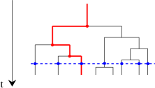
Let us consider a population of cells as shown in Fig. 1, which grow by division into only two offsprings at the end of each cell cycle. This population dynamics can be studied at three distinct levels : the lineage level (red), the population snapshot (blue) and the tree level which includes the complete phylogeny Lin and Amir (2017).
In the following, we shall introduce two different averages corresponding to the tree and lineage levels, which are defined for a fixed initial time and final time of the dynamics of the population. For a tree average, we consider all the branches of the tree including all the cells still present at time and which will divide only after the time . This tree distribution puts an equal weight on the lineages which end at time and from that point, it goes backward in time towards the original ancestor from which the population originated. For this reason, this distribution is known in the literature under the name of retrospective distribution Sughiyama et al. (2015) and is equivalently an average over histories, i.e. backward lineages Thomas (2017). In contrast to this, what we call in this paper a lineage average, corresponds to an average done over forward lineages, which go forward in time from the original ancestor of the colony towards its final state at time .
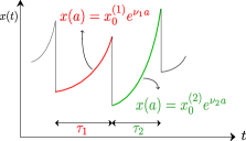
For bacteria such as E. coli growing in a rich medium, each cell cycle is well described by an exponential growth phase Brenner et al. (2015), which for the cell cycle can be parametrized by only three random variables shown in Fig. 2: the size at birth , the growth rate and the generation time .
III Results for size-controlled models
III.1 Definition of size-controlled models
Let us first consider a model with size-dependent division rate. The evolution of the number of cells of size and single cell growth rate at time , with , obeys the equation Hall (1991); Robert et al. (2014):
where is the division rate and is the probability for a newborn cell to have parameters y given that the mother cell has parameters . By integrating Eq. (III.1) over y using the condition , a deterministic equation of evolution of the total population is obtained.
The instantaneous growth rate of the population is defined as , while the growth rate of the total volume of the cells is with . When a steady state for the variable y is reached, both and become independent of time and equal to each other Lin and Amir (2017).
If instead of the full population, we consider the dynamics at the lineage level, the natural quantity to study is the probability density of the cell to have size and growth rate at time , , which satisfies the evolution equation
Note the difference with Eq. (III.1) due to the absence of the factor in front of the integral, rendering normalizable at any time, .
III.2 Fluctuation theorem for dynamical activity
We now address the problem of connecting lineage to tree or population snapshot statistics in models with size control. The evolution of a given cell from time 0 to the time is encoded in the trajectory .
For the case of size-controlled model, we derive in Appendices A, path probabilities representations at the population and lineage levels, which are given by (A.2) and (A.1) respectively. Comparing these two expressions, we see that a possible way to bring both distributions “closer” together, is to multiply the division rate at the lineage level by the factor , and to consider a lineage starting from the same initial condition as that of the population.
Then, we introduce the dynamical activity , which quantifies the activity of cell divisions, and the time averaged population growth rate
| (3) |
After multiplying the relation mentioned above between path probabilities by an arbitrary trajectory-dependent observable , and after taking the average, for the special case where , one obtains the following fluctuation relation :
| (4) |
where denotes a tree average generated by the original dynamics with a division rate while denotes a lineage average with a modified dynamics that has a division rate . The reason for this modified division rate is that each cell divides into cells, as a result a factor two appears at the population level in Eq. (III.1), which is absent for the corresponding equation at the lineage level. In the particular case where the observable only depends on instead of the full trajectory , Eq. (4) relates the lineage level to the population snapshot level instead of the tree level. The mapping also requires that the original and the modified dynamics start with the same initial condition , defined here in terms of cell size and growth rate.
For the specific choice , Eq. (4) leads to Crooks-like relation Crooks (2000):
| (5) |
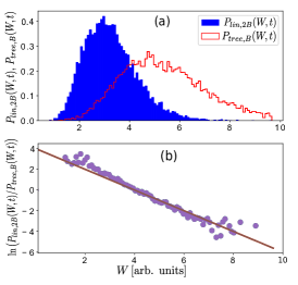
which relates the distribution of dynamical activity at time in a tree (resp. in a lineage): (resp. ). This relation is illustrated in Fig. 3 for a population of cells growing with a constant single cell growth rate . Numerically, instead of working directly with Eq. (III.1), we simulate an equivalent Langevin equation, which accounts for deterministic growth with the rate and stochastic cell divisions with a rate . In the simulation, the division has been assumed to be symmetric and the single cell growth constant, which corresponds to the particular choice of . Note that this dynamics bears some similarity to that of stochastic resetting introduced in Ref. Evans and Majumdar (2011), with the difference that in our case the resetting of the size is relative to the current size before division, while in this reference the resetting was to a constant position. Another important difference is the absence of diffusion in our model.
We have used normalized units of time and size, so that and in these units. Since , , the two distributions measured at the time cross as expected at (Fig. 3(a)). Fig. 3(b) confirms that the slope of the log-ratio of the two probability distributions is indeed as expected from Eq. (5).
Let us emphasize the following points concerning our first main result: This fluctuation relation is very general, it holds whether or not the single cell growth rate fluctuates, i.e., for arbitrary forms of the kernel and arbitrary division rate . There is no requirement that the population should be stationary neither at time nor at time . Further, it generalizes to the case that each cell has offsprings instead of two, provided that this number is independent on the state of the system y and that the modified lineage dynamics has a division rate , as shown in Appendix A.3.
The normalization of in (5) leads to the relation:
| (6) |
which could be used either to infer the population growth rate from lineage trajectories or to infer the form of the division rate using lineage and population trajectories Doumic et al. (2009). In the next subsection below, we provide such a numerical illustration.
III.3 Application to the determination of a population growth rate
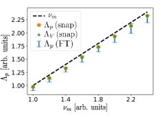
Since the variability of single cell growth rate is known to be important experimentally Brenner et al. (2015), we now discuss its role on the population growth rate in light of our results. A simple way to study this question in a simulation is to assume that the single cell growth rate is distributed according to a normal distribution of mean and variance . This is what we have done in Fig. 4, where a division rate of the form has been used. Although the values taken by are then uncorrelated from one division to the next, correlations between the mother and daugther generation times are still present due to the size dependence of the division rate. This figure compares several determinations of the population growth rate as function of . In the absence of variability where , we have , which is shown as a black dashed line in the figure. In the presence of variability, this figure confirms that the growth rate of the total volume equals the growth rate of the population where both of them have been measured from the statistics of the final population at a fixed time. Importantly, such a determination of the population growth rate also agrees (within errors bars) with the one based on Eq. (6) using lineage trajectories. Therefore, this shows that Eq. (6) could be used as a numerical method to determine a population growth rate based on lineage statistics.
Another striking feature of Fig. 4 is that regardless of the determination of , all the points are below the dashed line. The interpretation is that in a snapshot at time , it is less likely to see cells with a short generation time (corresponding to large single cell growth rates), therefore the distribution is biased towards small single cell growth rate Lin and Amir (2017). Since the population growth rate generally increases with respect to the single cell growth rate , this bias leads to a decrease of the population growth rate with respect to the case of no variability in the single cell growth rate.
As mentioned in the introduction, the fluctuation relation of Eq. (4) includes in itself a statistical biais: when choosing uniformly one individual in a population, an individual belonging to a lineage with prolific ancestors is more likely to be chosen, as a result, the jump rate on a lineage must be multiplied by the mean number of offsprings. Although variability in the single cell growth rate also introduces a form of statistical bias as explained above, the biais is not exactly the same one as that contained in the fluctuation relation. In any case, we would like to point out a comprehensive theoretical study on the effect of variability on the population growth rate, namely Olivier (2017). This study confirms that in the case of size models with i.i.d. single cell growth rates, variability indeed lowers the Malthusian growth rate as observed in figure 4. This work also discusses age models, with and without correlations in single cell growth rates, and concludes that in general, variability may lead to either a positive or negative trend on the population growth rate.
III.4 Consequences for the distribution of generation times
An important quantity in population dynamics is the distribution of generation times . This quantity can be evaluated from the observable Wakamoto et al. (2011):
| (7) |
where the index runs over all the cell cycles which have appeared in the trajectory that starts from to final time . This observable can be evaluated either on a lineage or on a tree. By reporting as the observable in Eq. (4), one deduces the relation
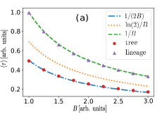
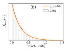
| (8) |
where a summation over the random variable and a dependence on the final time are implicit. In the particular case where the division rate is constant, and therefore . In this case, the generation time distribution in a lineage is the simple exponential with mean . It follows that with mean . Fig. 5 confirms that the distribution of generation times has the expected properties.
IV A second fluctuation theorem to relate lineage and tree statistics
When the division rate is not constant, the distribution of generation times will no longer be exponential, but we may still wonder how mean generation times observed at the lineage and tree levels compare to each other. In order to address this issue, we derive a different fluctuation theorem that connects this time the lineage and tree statistics with the same division rate . More precisely, it follows from a direct comparison of (A.2) and (A.1) taking again . Since the division rate is the same in both probability distributions, we stick to the notations introduced above, except that now the index will be omitted.
This allows to write
| (9) |
Now, by multiplying the above relation by an arbitrary trajectory-observable and taking , we obtain:
| (10) |
where counts as in Eq. (7) the number of divisions.
In the particular case where , Eq. (10) leads upon averaging, to a relation between the joint probability distributions of size, growth rate and number of divisions at the lineage and tree levels Nozoe et al. (2017):
| (11) |
which we call a local fluctuation relation. Averages over lineages within a population can be carried out with respect to either a chronological or to a retrospective distribution Sughiyama et al. (2015); Kobayashi and Sughiyama (2015); Wakamoto et al. (2011), which correspond respectively to our lineage and tree probability distributions. Let us briefly comment on a connection to a discussion presented in Ref. Nozoe et al. (2017). Elimination of in Eq. (11) leads to a fluctuation theorem only involving phenotypic traits and :
| (12) |
where we have introduced the probability of the number of division events conditioned on size and growth rate at the lineage level, and the equivalent of the “fitness landscape” of Ref. Nozoe et al. (2017) reads
| (13) |
By summing over in Eq. (11), one obtains
| (14) |
in terms of a function called “fitness landscape” in Ref. Nozoe et al. (2017). Eqs. (11)-(14) show that the knowledge of the two phenotypic probability distributions and can be used to infer a fitness function for size and growth rate.
IV.1 Inequalities for mean generation times
Let us also introduce the Kullback-Leibler divergence between two probabilities and :
| (15) |
Using the fluctuation relation of Eq. (9), we obtain
| (16) |
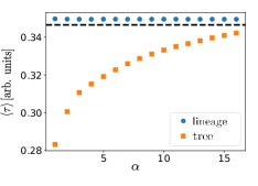
On large times , we can use the relation , which together with the definition of the population doubling time , leads to the right inequality in
| (17) |
while the left inequality follows very similarly using .
In the case that is constant shown in Fig. 5a, Eq. (17) is trivially satisfied. For non-constant of the form , the inequalities are verified numerically in Fig. 6. This figure shows that the mean generation time for lineage (resp. tree) approaches the doubling time in the limit of large , because in this limit the distribution of generation times becomes peaked at .
IV.2 Illustration of the inequalities based on experimental data
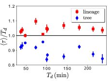
In this section, we present an illustration of the above inequalities, namely Eq. (17), using the experimental data of Hashimoto et al. Hashimoto et al. (2016). In this experiment, the single-cell growth dynamics of a population of E. coli placed in a constant environment has been tracked in a flow cytometer. From an analysis of single cell lineages, this experiment yields measurements of the population doubling time, together with the two mean generation times discussed above. The terminology used in this paper is different from the one we have introduced here but one can show that the distributions and introduced in that work correspond to what we call the lineage and tree distributions, respectively.
In the figure 3B of the main text of Hashimoto et al. (2016), the mean generation time along a lineage is shown as a function of the population doubling time for various bacteria strains, which illustrates the right inequality of Eq. (17). Fortunately, in the Suppl. Mat. of the paper, the data needed to plot the tree average is also given. For this reason, we show in Fig. 7, the combined data which illustrates both inequalities of Eq. (17).
This data has been interpreted in the framework of age-controlled model, assuming negligible mother-daughter correlations, which the authors have checked with their data Hashimoto et al. (2016). They have also shown theoretically, as we also find in the next section devoted to age models, that Eq. (17) hold for age-controlled model assuming no mother-daughter correlations. The important point we would like to make here is that this experimental data shown in Fig. 7 is also fully compatible with our predictions for size control models according to our Eq. (17). The strength of our derivation lies precisely in the fact that this result holds for a broad class of size-controlled models, without having to prescribe a precise form of the division rate or of the kernel .
V Results for age-controlled models
V.1 Definition of age-controlled models
When the division rate depends on the age of the cells instead of their size, the structure of the model is rather different from that of the previous subsection. Let us now introduce a further distinction between two types of age models. In the first type, the interdivision times of mother and daughter cells are uncorrelated, and the division rate is determined by the age of the cells only. Such a model is usually termed independent generation times (IGT) model or Bellmann-Harris process Kimmel and Axelrod (2015). In a second type of models, the division rate may depend on other variables besides the age, and as a result, mother-daughter correlations will be present. Although many results for IGT models have already appeared in the literature, it is needed to go through them in order to understand what changes when correlations are present.
In the case of the IGT type of models, the density of cells having age in the population at time , , satisfies the evolution equation
| (18) |
with the boundary condition:
| (19) |
As before, denotes the age-dependent division rate. The physical interpretation of the boundary condition (19) is clear: Each dividing cell gives rise to two newborn cells (i.e. two cells with age ). The total number of cells in the population at time follows by integration of the density, .
As in the case of size control, lineage dynamics can be directly encoded in the evolution of the age distribution. Such dynamics reads
| (20) |
which is complemented by the boundary condition:
| (21) |
so that probability is conserved and is normalized.
In a second type of models, correlations in the inter-division times are accounted for by adding an extra dependence of the division rate on the growth rate, , while introducing at the same time correlations between the growth rate of mother and daughter cells. The model then reads
| (22) |
| (23) |
at the population level, and
| (24) |
| (25) |
at the lineage level.
V.2 Generation time distribution
Beyond cell size control models, one can also consider age models, which may have or not mother-daughter correlations. Let us first consider the case where correlations are absent, the so-called IGT model, and let us focus on the distribution of generation times either in a lineage or in a population.
As in the case of size control, lineage dynamics of age-structured models can be directly encoded in the evolution of the age distribution, as prescribed by Eqs. (20) and (21). Let us consider steady-state conditions:
| (26) |
| (27) |
A nice feature of age models is that the generation-time distribution can be accessed directly. This is so because generation time distribution is the age distribution of the dividing cells. We proceed to compute this distribution for individual lineages in age-structured IGT models. First, note that from (26) immediately follows that
| (28) |
Relying on the relation between generation time distribution and age distribution of dividing cells, we can write
| (29) |
Now in order to obtain the distribution of generation times at the population level, we start from Eqs. (18) and (19). Again, we focus on stationary conditions for which the total number of cells in the population grows exponentially, as . In that case, de density can be written in terms of the stationary probability density of cells with a given age as , where is the stationary age distribution of the population. We have:
| (30) |
with the boundary condition:
| (31) |
It is worth noting that normalization of in (30), leads, using (31), to the following identity
| (32) |
We can now proceed to compute the generation time distribution, by computing the age distribution of dividing cells. We have first for the stationary distribution from (30):
| (33) |
where we have also used (32). On passing by, we highlight an important relation for IGT models obtained from the normalization of in Eq. (V.2):
| (34) |
We can now calculate the generation time distribution, which reads
| (35) |
Reading now from the result for the lineage, Eq. (V.2), we obtain :
| (36) |
which corresponds to the result derived in Ref Hashimoto et al. (2016) with the identification of their generation time distribution (resp. ) with our distributions (resp. ).
Using Eq. (36) we have, for instance:
| (37) |
where as usual the population doubling time reads . It is straightforward to prove the second inequality using the same technique. We then conclude that for IGT models, one has the same result as obtained for size structured populations in Eq. (17), i.e.,
| (38) |
V.3 Beyond uncorrelated age models
In view of the result of previous section, it is then natural to ask what happens in the more complex case in which mother-daughter correlations are present. In appendix B, we derived a generalization of Eq. (36) for that case, namely:
| (39) |
where (resp. ) represent the growth rate distributions of newborn cells at the lineage (resp. tree level). The presence of these two new probability distributions is entirely due to mother-daughter correlations. As a result, the inequalities (17) (identical to (38)) do not necessarily hold for age models with correlations. An example where they are indeed violated can be found in the model with correlated generation times studied in Ref. Amir and Lin (2018) in some range of parameters.
VI Conclusion
In conclusion, we have established several fluctuation relations which relate observables measured at the lineage and tree levels. We have deduced from the second fluctuation relation that mean generation times in a lineage are larger than the population doubling time, while mean generation times in a tree are smaller than the population doubling time. We have found that the experimental data of Hashimoto et al. fully confirm this observation Hashimoto et al. (2016). We conclude from this that this data is compatible either with the uncorrelated age-models used by these authors to analyze their data, or with the class of cell size control mechanisms considered in this paper.
Our approach being general, it could be extended to cover more complex cases such asymmetric divisions relevant for yeast cells, non-exponential regimes of growth, relevant for eukariots and other mechanisms of cell aging Stewart et al. (2005). While we have mainly focused on the control of the size variable, extension of this formalism to other variables not directly linked to cell size is possible, one choice being for instance the protein copy numbers Brenner et al. (2015); Thomas (2017).
We also find that the variability of single cell growth has a negative impact on the population growth rate in the absence of mother-daughter growth-rate correlations when the division rate is . A positive impact due to correlations in the inter-division times has been reported in some other study Amir and Lin (2018), while more generally a positive or negative impact should be expected depending on the form of the division rate Olivier (2017). All these recent results suggest that generation times are under a strong evolutionary pressure in which single cell variability and correlations over generations Rivoire and Leibler (2014) play an important role.
In the future, we would like to study systems where the division rate is controlled simultaneosly by the size and the age of the cell, which represents a situation of major biological relevance Osella et al. (2014). Finally, while this work was under review, two new studies of cell growth dynamics have appeared, which relate either to our pathwise formulation Sughiyama et al. (2019) or to our analysis of generation time distributions Jafarpour et al. (2018).
Acknowledgements.
R.G.G. was supported by the Agence Nationale de la Recherche (ANR-16-CE11-0026-03) and by Labex CelTisPhysBio (ANR-10-LBX-0038). We would like to thank E. Braun, L. Robert, A. Olivier, T. J. Kobayashi and Y. Wakamoto for stimulating discussions.Appendix A Path integral representation of the dynamics for size-controlled models
A.1 Population level
Let us start by building a path integral representation associated to the evolution of the number density of cells in the population case, Eq. (III.1). Here, we will allow for an arbitrary number of offsprings for generality, although only was considered above. We emphasize that should be independent of the state of the system. Let us treat the following term
| (40) |
in Eq. (III.1) as a perturbation. The growth propagator of the unperturbed dynamics is such that
| (41) |
with initial condition . Then using these equations, one can check that
| (42) |
is equivalent to the initial problem given in Eq. (III.1). By explicitly using the definition of from Eq. (40), one obtains
| (43) |
which allows to find an explicit solution for iteratively.
The explicit solution of Eq. (41) is
| (44) |
which allows us to write:
| (45) |
or more compactly:
| (46) |
where trajectories explicity appearing in the exponential in the r.h.s. of (A.1) are given as , and , for , while . In our notations, and . In addition, the transition matrix is given as .
The last step now consists in noticing that the object propagating trajectories from up to time in (A.1) is not yet a path probability because it is not properly normalized. To deal with this issue it is good to pass from number densisites to population-level probability densities, , and . We can now write in terms of these quantities:
| (47) |
where the object
| (48) |
is now properly normalized and can be identified with the correct path propability generating averages of all observables related to the number density at the population level. We have added a subscript to indicate that the division rate is given by . This will be important later in the derivation of fluctuation theorems. Note that when passing from densities to probability densities, a new term has appeared in the argument of the exponential namely , which is connected to the population growth rate, , by Eq. (3).
A.2 Lineage level
The starting point to derive the path probability for lineage observables is the evolution equation for the probability density of size and growth rate, Eq. (III.1) Except for the absence of the factor two in front of the integral, the structure of the equations are the same and the derivation follows along exactly as in the population case. We provide the final result:
| (49) |
which can be readily shown to be properly normalized. Here is the distribution of initial conditions for the lineage. Note that we have introduced , which could be different from the introduced earlier as the initial condition of the population.
A.3 Derivation of fluctuation relations
We can now compare path probabilities representations at the population and lineage levels given by (A.2) and (A.1) with each other. We see that a possible way to bring both distributions “closer” together, is to multiply the division rate at the lineage level by the factor , and to consider a lineage starting from the same initial condition as that of the population. A possible choice of this initial condition consists, for instance, in considering a population dynamics starting from a single cell.
Appendix B Fluctuation theorem for correlated age models
B.1 Lineage dynamics
We now consider models in which interdivision times are correlated. The natural way in which these correlations arise is by inter-cell-cycle growth-rate fluctuations, as given by Eqs. (24) and (25). Growth-rate correlations are encoded in , which is a properly normalized conditional probability. Again, we will focus on stationary conditions. It is simple to see from (24) that one can formally write the stationary distribution as:
| (52) |
To determine , we use (25) and (52):
| (53) |
from where we get the following integral equation:
| (54) |
The generation time distribution can now be determined, again, as the age-distribution of dividing cells. It is worth considering slightly more general object, i.e., the joint probability distribution of interdivision time and growth rate
| (55) |
This result can be written in a more illuminating way by noticing that the growth rate distribution of newborn cells can be identified as
| (56) |
Furthermore, due to the linearity of Eq. (54), and the fact that differs from only in a multiplicative constant, we have that satisfies
| (57) |
These observations then lead to the final result:
| (58) |
B.2 Population dynamics
Let us now consider the population level. The stationary equation for the population age distribution reads
| (59) |
with boundary condition
| (60) |
We then have
| (61) |
Note that the normalization of gives the following condition:
| (62) |
where we have used (61) and introduced the function
| (63) |
We can thus write for the growth rate of the population:
| (64) |
On the other hand, integrating directly in (61), we get
| (65) |
so we have
| (66) |
As before, we can find an equation for using (60) and the solution for , Eq. (61):
| (67) |
so, we then have
| (68) |
Let us now write the joint probability distribution of interdivision times and single-cell growth rate:
| (69) |
The condition (66) implies that , where
| (70) |
can be identified, as we did in the lineage case, with the growth rate distribution of newborn cells, now at the tree level. We then have:
| (71) |
Note once more that the linearity of Eq. (68) and the fact that and differ only on a multiplicative factor, lead to the equation satisfied by :
| (72) |
If we now compare (B.2) and (58), we readily obtain Eq. (39). Before closing this paragraph some comments are in order. First, note that as Eqs. (57) and (72) are clearly different, one has . Nevertheless, in absence of fluctuations, when , we have . To illustrate this, let us consider, for instance, a population starting from a single cell with growth rate . As the growth rate remains the same in all cell cycles, we have at all times. Then, Eq. (57) becomes tautological, while Eq. (72) leads to the identity
| (73) |
which is precisely the relation (34) found for IGT models (recall the definition of , (63)).
B.3 Inequalities in correlated age models
Let us now analyze the consequences of the generalized relation (39) for the inequalities. We have, for instance:
| (74) |
where is the marginal distribution of the growth rate of the dividing cells. This result implies, in particular, that
| (75) |
References
- Koch (2001) A. Koch, Bacterial growth and form (Springer, 2001).
- Willis and Huang (2017) L. Willis and K. Huang, Nat. Rev. Microbiol. 15, 606 (2017).
- Amir (2014) A. Amir, Phys. Rev. Lett. 112, 208102 (2014).
- Robert et al. (2014) L. Robert, M. Hoffmann, N. Krell, S. Aymerich, J. Robert, and M. Doumic, BMC Biol. 12, 17 (2014).
- Taheri-Araghi et al. (2015) S. Taheri-Araghi, S. Bradde, J. T. Sauls, N. S. Hill, P. A. Levin, J. Paulsson, M. Vergassola, and S. Jun, Curr. Biol. 25, 385 (2015).
- Grilli et al. (2017) J. Grilli, M. Osella, A. S. Kennard, and M. C. Lagomarsino, Phys. Rev. E 95, 032411 (2017).
- Campos et al. (2014) M. Campos, I. V. Surovtsev, S. Kato, A. Paintdakhi, B. Beltran, S. E. Ebmeier, and C. Jacobs-Wagner, Cell 159, 1433 (2014).
- Powell (1956) E. O. Powell, Microbiology 15, 492 (1956).
- Kimmel and Axelrod (2015) M. Kimmel and D. E. Axelrod, Branching Processes in Biology (Springer, 2015).
- Hashimoto et al. (2016) M. Hashimoto, T. Nozoe, H. Nakaoka, R. Okura, S. Akiyoshi, K. Kaneko, E. Kussell, and Y. Wakamoto, Proc. Natl. Acad. Sci. 113, 3251 (2016).
- Hall (1991) A. J. Hall, Steady Size Distributions in Cell Populations, Ph.D. thesis, Massey University (1991).
- Kobayashi and Sughiyama (2015) T. J. Kobayashi and Y. Sughiyama, Phys. Rev. Lett. 115, 238102 (2015).
- Sughiyama et al. (2015) Y. Sughiyama, T. J. Kobayashi, K. Tsumura, and K. Aihara, Phys. Rev. E 91, 032120 (2015).
- Crooks (2000) G. E. Crooks, Phys. Rev. E 61, 2361 (2000).
- Nemoto et al. (2016) T. Nemoto, F. Bouchet, R. L. Jack, and V. Lecomte, Phys. Rev. E 93, 062123 (2016).
- Giardinà et al. (2006) C. Giardinà, J. Kurchan, and L. Peliti, Phys. Rev. Lett. 96, 120603 (2006).
- Bansaye et al. (2011) V. Bansaye, J.-F. Delmas, L. Marsalle, and V. C. Tran, Ann. Appl. Probab. 21, 2263 (2011).
- Nozoe et al. (2017) T. Nozoe, E. Kussell, and Y. Wakamoto, PLoS Genet. 13, 1 (2017).
- Lin and Amir (2017) J. Lin and A. Amir, Cell Systems 5, 358 (2017).
- Thomas (2017) P. Thomas, J. R. Soc. Interface 14, 20170467 (2017).
- Brenner et al. (2015) N. Brenner, E. Braun, A. Yoney, L. Susman, J. Rotella, and H. Salman, Eur. Phys. J. E 38, 102 (2015).
- Evans and Majumdar (2011) M. R. Evans and S. N. Majumdar, Phys. Rev. Lett. 106, 160601 (2011).
- Doumic et al. (2009) M. Doumic, B. Perthame, and J. P. Zubelli, Inverse Probl. 25, 045008 (2009).
- Olivier (2017) A. Olivier, Am. Inst. of Math. Sci. 10, 481 (2017).
- Wakamoto et al. (2011) Y. Wakamoto, A. Y. Grosberg, and E. Kussell, Evolution 66, 115 (2011).
- Amir and Lin (2018) A. Amir and J. Lin, “Population growth with correlated generation times at the single-cell level,” (2018), arxiv: 1806.02818.
- Stewart et al. (2005) E. J. Stewart, R. Madden, G. Paul, and F. Taddei, PLOS Biology 3 (2005).
- Rivoire and Leibler (2014) O. Rivoire and S. Leibler, Proc. Natl. Acad. Sci. U.S.A. 111, 1940 (2014).
- Osella et al. (2014) M. Osella, E. Nugent, and M. Cosentino Lagomarsino, Proc. Natl. Acad. Sci. U.S.A. 111, 3431 (2014).
- Sughiyama et al. (2019) Y. Sughiyama, S. Nakashima, and T. J. Kobayashi, Phys. Rev. E 99, 012413 (2019).
- Jafarpour et al. (2018) F. Jafarpour, C. S. Wright, H. Gudjonson, J. Riebling, E. Dawson, K. Lo, A. Fiebig, S. Crosson, A. R. Dinner, and S. Iyer-Biswas, Phys. Rev. X 8, 021007 (2018).