A Monte Carlo Framework for Rendering Speckle Statistics in Scattering Media
Abstract.
We present a Monte Carlo rendering framework for the physically-accurate simulation of speckle patterns arising from volumetric scattering of coherent waves. These noise-like patterns are characterized by strong statistical properties, such as the so-called memory effect, which are at the core of imaging techniques for applications as diverse as tissue imaging, motion tracking, and non-line-of-sight imaging. Our framework allows for these properties to be replicated computationally, in a way that is orders of magnitude more efficient than alternatives based on directly solving the wave equations. At the core of our framework is a path-space formulation for the covariance of speckle patterns arising from a scattering volume, which we derive from first principles. We use this formulation to develop two Monte Carlo rendering algorithms, for computing speckle covariance as well as directly speckle fields. While approaches based on wave equation solvers require knowing the microscopic position of wavelength-sized scatterers, our approach takes as input only bulk parameters describing the statistical distribution of these scatterers inside a volume. We validate the accuracy of our framework by comparing against speckle patterns simulated using wave equation solvers, use it to simulate memory effect observations that were previously only possible through lab measurements, and demonstrate its applicability for computational imaging tasks.
1. Introduction
Scattering refers to the propagation of radiation (for instance, light or sound) in non-uniform media, composed of small discrete scatterers, usually particles of varying refractive properties: As an incident wave propagates through the medium, it will interact with scatterers multiple times, and each such interaction will change the wave’s shape. Scattering is commonly encountered when visible light interacts with a large variety of materials, for instance biological tissues, minerals, the atmosphere and clouds, cosmetics, and many industrial chemicals. As a result of the ubiquity of scattering, its study has attracted numerous research efforts in computer graphics and vision, and much more broadly in medical imaging, remote sensing, seismic imaging, and almost any field of natural science.
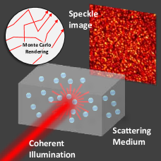
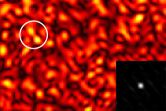
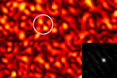
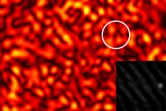
The appearance of scattering materials is qualitatively very different, depending on whether they are imaged under incoherent or coherent conditions. In the incoherent case, scaterring results in images with smoothly-varying intensity distributions, often referred to as translucent appearance. By contrast, under coherent imaging conditions, the appearance of scattering materials is characterized by speckles, that is, pseudo-random high variations in the output waves and captured intensity images. Speckles have been the subject of multiple textbooks (Goodman, 2007; Erf, 1978; Jacquot and Fournier, 2000; Kaufmann, 2011), as despite their random structure, they have strong statistical properties that are characteristic of the underlying material. For example, a remarkable property of speckles is the memory effect: speckle fields produced under small perturbations in imaging parameters (e.g., change in illumination direction) are highly correlated shifted versions of each other (see Fig. 1). These speckle statistics have received strong attention since the invention of coherent laser illumination (Li and Genack, 1994; Berkovits and Feng, 1994; Feng et al., 1988; Freund et al., 1988), and are at the core of a large array of imaging techniques, with applications as diverse as motion tracking, estimating blood flow, looking around the corner, and seeing through scattering layers.
Unfortunately, and in stark contrast with the incoherent case, our ability to accurately simulate scattering in the coherent case is severely limited. Available algorithms generally fall into two categories. The first category consists of algorithms that compute output waves by numerically solving Maxwell’s equations (Thierry et al., 2015; Yee, 1966; Treeby and Cox., 2010). These algorithms are physically accurate, but require as input the microscopic structure of the scattering medium, that is, knowledge of the exact (at sub-wavelength accuracy) locations of all scatterers in the medium. Even when such a microscopic characterization is available (e.g., specific samples examined with a microscope, or volumes with hallucinated scatterer locations), the high computational complexity of wave equation solvers makes them inapplicable for volumes larger than a few hundred cubic wavelengths, or containing more than a few hundred scatterers. The second category consists of approximate Monte Carlo rendering algorithms (Xu, 2004; Sawicki et al., 2008), which accumulate the complex throughput (amplitude and phase) of paths sampled using standard volumetric path tracing. These algorithms are efficient, but cannot reproduce statistical properties of real speckles such as the memory effect. The lack of speckle rendering algorithms that are both physically accurate and computationally efficient is a significant obstacle in the wide range of fields interested in coherent imaging of scattering volumes. Symptomatic of these shortcomings of existing rendering tools is the fact that the only reliable way for estimating the memory effect has been by conducting painstaking optical lab experiments (Schott et al., 2015).
In this paper, we change this state of affairs by developing a Monte Carlo framework for rendering speckles in volumetric scattering. Our framework builds on the following insight: Due to the central limit theorem, speckles are instances of a multivariate Gaussian distribution (Goodman, 2007). Therefore, it is sufficient to model their (scene and material-dependent) mean and covariance. To achieve this, we draw inspiration from Monte Carlo volume rendering algorithms for the incoherent case: These algorithms treat the scattering medium as a continuous volume, inside which light can scatter randomly at any location. Given bulk parameters characterizing the statistical distribution of scatterers in the medium, Monte Carlo algorithms synthesize images corresponding to the average distribution of scattered light across all scatterer instantiations that can be generated from the bulk parameters (Moon et al., 2007). This macroscopic view of the medium enables efficient rendering, without the need to know and simulate the medium’s microscopic structure.
To extend this approach to the coherent case, we begin by deriving from first principles a new path-integral formulation (Veach, 1997) for the propagation of coherent light inside a scattering medium, which accurately encapsulates the first-order and second-order statistics of resulting speckle patterns. From this formulation, we derive two Monte Carlo rendering algorithms. The first algorithm estimates speckle covariance, which, together with an estimate of speckle mean obtained using a closed-form expression, can be subsequently used to sample multiple speckle images. The second algorithm directly simulates a physically-accurate speckle image, and operates by having sampled paths contribute to multiple pixels in a way that produces accurate speckle statistics. Both algorithms take as input only bulk macroscopic scattering parameters, as in the incoherent case. We validate our theory and algorithms in a few ways: First, we show that our approach can closely match “groundtruth” speckle estimates, obtained by averaging solutions of the wave equation across multiple particle instantiations, while also being orders of magnitude faster. Second, we show that our approach agrees with analytical formulas for speckle correlations derived for specific cases (e.g., diffusion). Finally, we show that our approach can accurately reproduce well-documented properties of speckles, such as the memory effect and coherent backscattering. We show example applications of our framework, including simulating speckle-based computational imaging techniques, and evaluating the extent of their applicability.
1.1. Why render speckle patterns?
There exist several imaging techniques that directly leverage second-order speckle statistics. Example applications include motion tracking (Jacquot and Rastogi, 1979; Jakobsen et al., 2012; Smith et al., 2017), looking around the corner (Freund, 1990; Katz et al., 2012; Batarseh et al., 2018), and seeing through (Katz et al., 2014; Bertolotti et al., 2012) or focusing through (Mosk et al., 2013; Nixon et al., 2013; Osnabrugge et al., 2017; Vellekoop and Aegerter, 2010) tissue and other scattering layers. Most of these imaging techniques rely on the memory effect of speckles, a fact that has motivated significant research on quantifying this effect for different materials. Existing computational approaches generally attempt to derive closed-form expressions for the memory effect (Akkermans and Montambaux, 2007; Baydoun et al., 2016; Dougherty et al., 1994; Osnabrugge et al., 2017; Freund and Eliyahu, 1992; Berkovits and Feng, 1994; Fried, 1982; Feng et al., 1988). Unfortunately, these expressions only hold under assumptions such as diffusion or the Fokker-Planck limits, restricting their applicability. As a result, it has generally been necessary to measure the memory effect empirically using involved optical setups (Schott et al., 2015; Yang et al., 2014; Mesradi et al., 2013). Our algorithm allows quantifying the memory effect for arbitrary scattering materials computationally, through accurate yet efficient simulations. This can significantly enhance our understanding of the applicability of memory effect techniques to different materials. Additionally, this new simulation capability can save considerable lab effort for tasks such as discovering optimal settings for computational imaging systems, and evaluating new imaging configurations.
The ability to efficiently render speckle patterns can facilitate the widespread adoption of data-driven approaches in fields where coherent imaging of scattering is common, such as tissue imaging and material science. Previously, the lack of physically-accurate simulation tools meant that training datasets had to be collected using lab measurements, an approach that is not scalable.
Finally, speckle statistics can be beneficial for inverse rendering, that is, retrieving material parameters from image measurements. While previous approaches use intensity measurements (Gkioulekas et al., 2013; Gkioulekas et al., 2016; Holodovski et al., 2016; Levis et al., 2015), measurements of speckle statistics may capture additional information and allow inverse rendering techniques to be applied in finer scales, where it is not possible to image without coherent effects.
2. Related Work
Monte Carlo rendering of wave optics effects has recently attracted increased attention in computer graphics. A primary focus has been on rendering diffraction and speckle effects generated by surface microgeometry (Yan et al., 2018; Stam, 1999; Cuypers et al., 2012; Werner et al., 2017; Yeh et al., 2013; Bergmann et al., 2016), without tackling volumetric scattering. Some approaches focusing on scattering and speckle effects can be found in the optics literature (Pan et al., 1995; Schmitt and Knüttel, 1997; Lu et al., 2004). For instance, Xu et al. (2004; 2008) modify volumetric path tracing, by tracking complex phase as a path is traced through the volume. By aggregating complex contributions from paths on the sensor, this technique produces images that resemble speckle patterns. However, because every pixel is rendered independently, this approach cannot reproduce spatial correlations between pixels. Additionally, it is impossible to use these approaches to reproduce correlations that exist across multiple illumination directions as in the memory effect.
There have been attempts to use Monte Carlo algorithms to evaluate various properties of coherence and partial coherence of light after propagating through a scattering tissue (Shen et al., 2017; Pierrat et al., 2005). Often these are based on using the radiative transfer equation (RTE) and intensity-based Monte Carlo rendering, then applying a Fourier transform on its result. Such approaches can be justified as a special case of our algorithm.
An important result in the study of speckle statistics, which can be used to derive Monte Carlo rendering algorithms, is the correlation transfer equation (CTE) (Ishimaru, 1999; Twersky, 1964; Dougherty et al., 1994). This integral equation extends the RTE, by modeling correlation of fields at different space points. As we show in Sec. 6.1, there are physical phenomena that are not accounted for by the CTE, such as coherent backscattering. While there exist some Monte Carlo rendering algorithms that take this effect into account (Sawicki et al., 2008; Ilyushin, 2012), they only simulate intensity and not general covariance. We revisit the derivation of the CTE and its underlying assumptions, aiming to derive a more general rendering framework that accurately models both covariance and coherent backscattering.
Our derivation is fundamentally based on supplanting the true scattering volume, consisting of multiple discrete scatterers at fixed locations, with a continuous volume where scattering can happen randomly at any location. This macroscopic treatment of scattering underlies all current Monte Carlo volume rendering algorithms, and has also been used to accelerate rendering of so-called discrete random media, where the scatterers can be arbitrarily large or dense (Moon et al., 2007; Müller et al., 2016; Meng et al., 2015). More recently, a number of works have used this approach to derive generalized versions of the RTE and Monte Carlo rendering algorithms, for media where the distribution of scatterer locations has spatial correlations, so-called non-exponential media (Bitterli et al., 2018; Jarabo et al., 2018; d’Eon, 2018b, a). Even though we focus exclusively on exponential media, our work provides the foundations for future investigations of Monte Carlo rendering of speckles in non-exponential media.
Finally, there is also research on temporal correlations in the presence of scatterer motion, e.g., in liquid dispersions (Dougherty et al., 1994). Many established techniques use these temporal speckle correlations to estimate flow (e.g., blood flow (Durduran et al., 2010)) and liquid composition parameters. Example techniques include diffusing wave spectroscopy (Pine et al., 1988), laser speckle contrast imaging (Boas and Yodh, 1997), and dynamic light scattering (Goldburg, 1999). Here we focus on spatial speckle correlations leaving these temporal effects for future work.
3. Modeling speckle statistics
 |
 |
 |
 |
 |
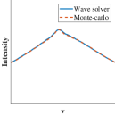 |
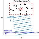
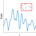
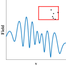
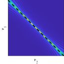
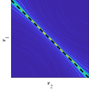
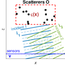
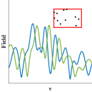
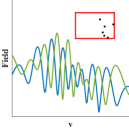
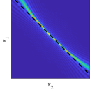
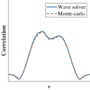
| (a) Setup with one illumination | (b) Sampled field 1 | (c) Sampled field 2 | (d) Wave solver cov | (e) MC covariance | (f) Diagonal plot from (d,e) |
 |
 |
 |
 |
 |
 |
| (g) Setup with two illuminations | (h) Sampled field 3 | (i) Sampled field 4 | (j) Wave solver cov | (k) MC covariance | (l) Diagonal plot from (j,k) |
Definitions and notation. We use bold letters for three-dimensional vectors (e.g., points ), with a circumflex for unit vectors (e.g., directions ). We also use for the unit vector from to . Illumination and imaging can be at either the near or the far field: Near-field illumination is an isotropic source at point , whereas far-field illumination is a directional plane wave source at direction ; and likewise for sensor points and directions . We often abuse the point notation for both the far-field and near-field cases, except where context requires otherwise. We also restrict discussion to unpolarized illumination.
We consider scattering volumes that satisfy four assumptions: First, they consist of scatterers with size comparable to the illumination wavelength, and which can therefore be considered infinitesimal. Second, the scatterers are far from each other, with an average pairwise distance (the mean free path) an order of magnitude larger than the wavelength. Third, the locations of scatterers are statistically independent. Fourth, scatterers scatter incident waves in a way that is invariant to rotation. These assumptions underly classical radiative transfer (Bitterli et al., 2018). To simplify notation, in the main paper we derive results assuming scatterers of a single type (same shape, size, and refractive index), and extend to the case of multiple types in Appendix 9.1. We denote by the, possibly spatially varying, density describing the distribution of scatterers in the medium. Finally, to simplify discussion, we do not model the interface of volume ; interface events (reflection and refraction) can generally be incorporated in our resulting rendering algorithms same as in regular volume rendering.
The scattered field. An incident wave of wavelength interacting with scatterers stimulates a scattered wave , which can be computed by solving the Helmholtz equation. When a single particle located at is illuminated from direction , the scattered wave at distance is,
| (1) |
The complex function is the scattering amplitude function, describing scattering at different angles. The scalar is known as the scattering cross-section, and accounts for the total energy scattered by the scatterer. Both quantities are a function of the wavelength and the scatterer’s shape, size, interior and exterior refractive index; for spherical scatterers, they can be computed using Mie theory (Bohren and Huffman, 1983; Frisvad et al., 2007). We note that the scattering amplitude function is often defined as the product . Here we separate the two terms and assume that integrates to 1.
We now consider the geometry illustrated in Fig. 2a: Scatterers are placed at locations , each sampled independently from the density . This configuration is illuminated from a source , and imaged with a sensor . Knowing the exact scatterer locations, we can solve the wave equation to obtain the complex-valued scattered field , which typically contains large fluctuations with a semi-random noise structure known as speckles (see flatland speckles in Fig. 2b,c).
Speckle statistics. Images modeled using the radiative transfer equation correspond to the intensity of the scattered field, averaged over all particle instantiations sampled from , as in Fig. 2f:
| (2) |
These incoherent intensity images are typically smooth, without speckles. This is because of the incoherent addition in Eq. (2): The expectation is formed by averaging intensities of waves, whereas speckles are the result of coherent addition of complex valued waves. To capture speckle statistics, we can begin with the speckle mean,
| (3) |
We can similarly define higher-order statistics of speckles. Of particular importance will be the speckle covariance,
| (4) |
where denotes complex conjugation. In this case, are two speckle fields generated by the same scatterer configuration , when illuminated by two incident waves from , and measured at two sensors . When the term from Eqs. (3) and (4) reduces to the intensity of Eq. (2). As we discuss in Sec. 4.1, the speckle mean can be computed using a closed-form expression; in fact, because the speckle mean is the aggregate of complex numbers of essentially randomly-varying phase, it is typically zero. Therefore, when characterizing speckle statistics, the most challenging part is computing the covariance.
Gaussianity of speckles. Before we discuss ways to compute the speckle mean and covariance, one may wonder whether it is necessary to consider higher-order speckle statistics. The answer, in general, is negative: Classical results in optics (Goodman, 2007) state that the space of solutions of the wave equation, for all particle configurations sampled from , follows a multivariate Gaussian distribution with scene-dependent mean and covariance. The Gaussianity results from the central limit theorem, as the particle locations are independent random variables. Consequently, the multivariate mean and covariance of Eqs. (3) and (4) provide sufficient statistics for speckle, and can be used to sample speckle patterns that are indistinguisable from patterns generated by specifying exact particle positions and solving the wave equation.
Computing speckle statistics. A straightforward approach for computing the speckle mean and covariance is to sample different scatterer configurations , solve the wave equation for each configuration, and then compute the empirical moments:
| (5) | |||
| (6) |
Fig. 2(d,k) shows speckle covariances evaluated with this procedure. Solving the wave equation is only tractable for very small number of particles (a few thousands), and this computational cost is further exacerbated by the need to repeat this process multiple times. Our goal is to devise Monte Carlo algorithms that can compute speckle covariance directly and much more efficiently.
Bulk parameters. Unlike wave equation solvers, our algorithms are not tied to a specific position of scatterers. Instead, they rely only on the distribution of scatterers in the medium, as well as their size, shape, and refractive properties. As in the radiative transfer literature, we describe these using the scattering, absorption, and extinction coefficients, respectively, defined as
| (7) | |||
| (8) |
where are the scattering and absorption cross-sections, denoting the energy scattered or absorbed upon interaction with one particle, is the radius of the particles, is the expected number of particles in a unit volume, and is the absorption coefficient of the containing medium. We also use the phase function, defined as , explaining our earlier choice of normalization for the scattering amplitude function. The above definitions consider only particles of a single type, but it is not hard to extend them to multiple particle types, see Appendix 9.1.
4. Path-space view of speckle statistics
In this section, we derive path-space expressions for the speckle mean and covariance. These expressions will form the basis for the Monte Carlo rendering algorithms of Sec. 5. We note that, traditionally in computer graphics, path-space expressions are derived by recursively expanding integral equations such as the surface and volume rendering equations. Here, we start directly with a path-space view, and discuss the relationship with an integral equation known as the correlation transfer equation (CTE) in Appendix 9.5.
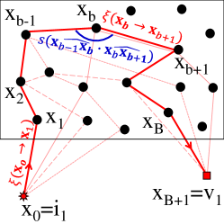
Fields as path sums. Our starting point is the classical theory of Twersky (1964): Given a configuration of particles, we can approximate the solution to the wave equation as the sum of contributions over all paths through . That is, consider the (enumerable) set of all ordered sequences:
| (9) |
where . Then, the scattered field can be expressed as
| (10) |
These paths are illustrated in Fig. 3. The complex throughput terms correspond to the amplitude and phase change at each segment on the path, accounting for the scattering amplitude and traveled length. They can be defined as
| (11) | ||||
| (12) |
The complex transmission terms account for phase change and radial decay between path vertices , defined for points at the near field and far field, respectively, as
| (13) |
Speckle statistics as path integrals. Using Eq. (10), we can now express the mean and covariance by averaging over all particle configurations that can be sampled from the density :
| (14) | |||
| (15) |
Note that, within the expectation, the summation is over paths through the same particle instantiation . By exchanging the order of expectation and summation in Eqs. (14) and (15), we have:
| (16) | |||
| (17) |
where now the space includes paths with vertices that can be anywhere in the volume , not only on fixed particle locations. Unlike , is not an enumerable space, thus summation is replaced with integration. The term is the probability that the path is included in the enumerable path space for some particle configuration sampled from ; similarly is the probability that all nodes on both are included in the same particle configuration .
In the following sections, we show that can be computed in closed form, and we greatly simplify the path integral for by characterizing the pairs of paths that have non-zero contributions.
4.1. The speckle mean
Evaluating the speckle mean is addressed by standard textbooks on scattering. We present these results here, starting from a more general case, which subsumes the computation of speckle mean. The general case will also be useful for computing speckle covariance in the next section.
We consider a particle at , illuminated from a wave with incident direction . As this wave scatters, we want to evaluate the average contribution of all paths starting at and arriving at a second point . The textbook result (Ishimaru, 1999; Mishchenko et al., 2006) states this average can be written as
| (18) |
where is defined as in Eq. (11). The term is defined in the near and far fields as the probability of getting from to without meeting other particles, and is equal to
| (19) |
For a homogeneous medium The factor in the exponent of Eq. (19) makes the square root of the attenuation term used in standard radiative transfer. Intuitively, this is because we deal with the field rather than intensity.
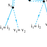
The main intuition behind Eq. (18) is that, as most paths contribute essentially random complex phases, they cancel each other out. Therefore, the total field from to equals the field that travels only along the direct path between the two points, attenuated by the exponentially decaying probability see Fig. 4(a).
Computing the speckle mean. We can now adapt this result for the case of the speckle mean of Eq. (16). If either the source or the sensor are at the near field, the speckle mean in Eq. (16) is a special case of Eq. (18). Being the mean of paths from to without conditioning on an incoming direction , we omit the term representing scattering, and express
| (20) |
compare Eq. (12) with Eq. (11) for the definition of . In Appendix 9.2, we show how to adjust this for the far field as well.
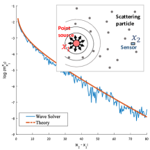
The main consequence of this section is that computing the speckle mean becomes a direct illumination problem, which can be solved analytically without the need for path integration. In Fig. 4(b), we numerically evaluate the speckle mean by averaging multiple solutions of the wave equation as in Eq. (5), showing a good agreement with the analytic formula of Eq. (20). We note that, as the speckle mean decays exponentially with the distance, in most cases it is negligible, making the computation of covariance the main challenge in simulating speckle. We discuss this next.
4.2. The speckle covariance
We have shown in Eq. (17) that the speckle covariance can be expressed as an integral over pairs of paths from to and from to . Unlike the mean, there is no closed-form expression for this integral. However, we can considerably simplify integration by characterizing the pairs of paths with non-zero integrand
| (21) |
and deriving a simple formula for for those pairs. Some of the arguments we use are also discussed in Mishchenko et al. (2006). Here, we formalize these arguments and extend them to accurately account for both speckle covariance and, as we see below, coherent back-scattering. Our end-product is a new path-integral expression for covariance that lends itself to Monte Carlo integration.
Valid pairs of paths. Intuitively, as is a complex number, if we aggregate contributions from different pairs of paths with very different phases, they will likely average to zero. The exception to this argument is cases where is not complex; this happens when every segment that appears in also appears in .
Consider, as in Fig. 5(a), the set of path pairs that have an arbitrary number of vertices, but share only vertices (in any order). Then, as in Sec. 4.1, we expect all the different path segments from to to average to the direct path between these points. In Appendix 9.3, we prove that indeed all path pairs with disjoint nodes collapse to their joint nodes, and the average contribution of all pairs of paths sharing nodes is
| (22) | |||
| (23) |
The complex volumetric throughput terms combine the volumetric attenuation of Eq. (19) with the complex throughput of Eqs. (11) and (12). They can be defined as
| (24) | ||||
| (25) |
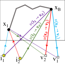
To recap, the complex volumetric throughput is a direct term, the product of three factors (i) the attenuation , (ii) the complex transmission , whose phase is the segment length, (iii) the scattering amplitude function of the direction turn (for paths of lengths ). The different terms are summarized in Fig. 6 .
We can therefore restrict the integration space of Eq. (17) to only pairs of paths that share all vertices except, perhaps, their endpoints. The contribution of such pairs, given by Eq. (22), is Markovian and can be computed analytically. Next, we further constrain the integration space, by examining when pairs of paths sharing the same vertices but in different order have non-zero contribution.
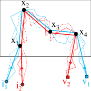
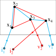
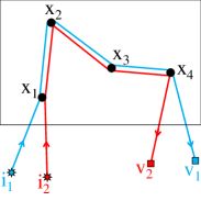
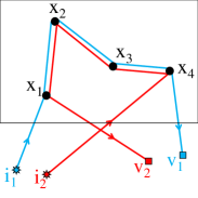
Vertex permutations. We now consider the contribution of a pair of paths sharing the same vertices , but in different permutations. The phase of the segment is proportional to the length of that segment. Permutations that do not trace the nodes in the same order have segments with different lengths (see Fig. 5b), and thus different phases. Intuitively, as in Sec. 4.1, they are likely to average to zero. However, for each ordered set of vertices , there is one important permutation for which this argument does not apply, as the central segments have the same length: the reversed permutation (Fig. 5c and 5d). Therefore, we need to consider contributions from pairs involving four paths (Mishchenko et al., 2006),
| (26) | |||||
The reversed paths are the cause of the well-documented phenomenon of coherent backscattering, which happens when one measures backscattering from a dense scattering volume, with far-field coherent illumination and sensing. When the backscattering and illumination directions are exactly equal, the scattered intensity is increased compared to nearby directions.
For intuition behind this effect, we first note that every particle instantiation that contains the path , also contains the reversed path ; that is, the forward and reversed paths are not independent events. Consequently, their contribution in Eq. (15) is rather than . We can compute the difference between these two terms, by considering the case , and neglecting the scattering amplitude . Then, the contribution of the forward and reversed paths becomes,
| (27) |
The shared intermediate segments have the same phase, therefore,
| (28) |
When is large, the average of the real term in Eq. (28) over all space points is low. However, when , as in coherent backscattering, the real term approaches unity, and therefore the total contribution is doubled. In other words, we get constructive interference between the forward and reversed paths.
Covariance path integral. We can now state concretely our path integral formulation for the speckle covariance: Consider the space of sub-paths , where each vertex can be everywhere in the volume , and . We write:
| (29) |
To define the integrand , we first form the four complete paths of Eq. (26), by connecting the forward and reversed versions of to the illumination and sensing conditions and . Then,
| (30) |
where the summands are defined in Eq. (22). By expanding the equations, and considering that now the pairs of paths have identical intermediate segments, we can rewrite this sum as
| (31) |
where is the standard radiometric throughput of , augmented by the scattering coefficients at the first and last vertices,
where the phase function was defined as . The 4 volumetric throughput connections of Eq. (31) are illustrated in Fig. 6, while is the volumetric throughput of the central segments (gray path in Fig. 6). As we see in the next section, the radiometric throughput term in Eq. (4.2) allows us to reuse path sampling algorithms from intensity rendering also for covariance rendering.
As the mean products are essentially the throughput contribution of paths from to and from to without shared nodes, we can drop this term from Eq. (29) by restricting the subpath space to paths of length , and define
| (33) |
We make two notes about the path integral formulation of Eq. (33). First, if one does not consider the reverse paths, then the resulting path-integral formulation is equivalent to what can be obtained from the correlation transfer equation (CTE). We discuss this in Appendix 9.5, and we also discuss how the Monte Carlo algorithms we derive in the next section compare to Monte Carlo algorithms derived from the CTE. In the evaluation of Sec. 6.1 we show that considering only forward paths can provide a good approximation in many cases; however, in cases where the sensor is close to collocated with the source, we should consider reversed paths as well.
Second, at the start of this section, we argued informally that pairs of paths with different permutations of do not contribute to covariance. In Appendix 9.4, we discuss this in more detail, and additionally show empirical evidence for ignoring these pairs. Likewise, the results in Sec. 6.1 show that accounting for only the forward and reversed path is accurate enough.
5. Monte Carlo rendering algorithms
We use the results of the previous section, to derive two Monte Carlo rendering algorithms. The first algorithm directly computes the speckle covariance, which we can use, together with an estimate of the speckle mean, to sample multiple speckle patterns. The second algorithm directly renders a speckle pattern, so that the empirical mean and covariance of multiple renderings is accurate.
5.1. Rendering speckle covariance
To approximate the covariance integral of Eq. (33), we define a strategy that samples sub-paths from a distribution that will be defined below. We use them to form a Monte Carlo estimate of the covariance as
| (34) |
The denominator of Eq. (34) is the sampling probability. As it is possible to independently sample both the forward and reserved version of a subpath, the total probability is .
|
|
The variance of the estimator in Eq. (34) reduces when is a good approximation to . As in Eq. (31) is Markovian, that is, expressed as a product of the contributions of individual segments, it lends itself to local sampling procedures. The sampling algorithm we use operates as follows: We sample the first vertex according to the volume density, using the probability distribution defined as:
| (35) |
For a homogeneous volume, reduces to the uniform density. Then, taking advantage of the fact that includes the radiometric throughput , we sample all other vertices of using volume path tracing (Veach, 1997; Dutré et al., 2006). Finally, as we trace , we perform next event estimation, connecting each vertex to the endpoints of the forward and reverse paths of Eq. (26), as illustrated in Fig. 6. The MC process is summarized in Algorithm 1, which also details how to handle single-scattering subpaths consisting of only one node.
5.2. Rendering speckle fields
As discussed in Sec. 3, the space of speckle images follows a multi-variate Gaussian distribution. Thus the mean and covariance provide sufficient statistics, which we can use to sample physically-correct speckle images, statistically indistinguishable from ones generated through an exact solution to the wave equation. However, with this approach, sampling an image of pixels requires that we first render an covariance matrix. While this is significantly more efficient than solving the wave equation, for large values this can still be costly. To address this, we present a second rendering algorithm that can synthesize speckle images directly.
Our starting point is the following observation: Let be the covariance matrix corresponding to all pairwise combinations of illumination and sensing conditions . Then, from Eqs. (33) and (31), we can write as an integral of rank-1 matrices,
| (37) |
where: is defined in Eq. (4.2), and is a vector with -th entry equal to the terms in Eq. (31) applied to and ,
| (38) |
Sampling a field from a multivariate Gaussian with a covariance as in Eq. (37) can be done by first initializing to the zero vector, then repeating the following: (i) Sample a subpath as in Algorithm 1. (ii) Sample a complex number of unit magnitude and random phase. (iii) Increment by (where is the square root of the scale in Eq. (36)). This is summarized in Algorithm 2, which also shows how to handle single-scattering subpaths consisting of length .
We elaborate on two details of the above procedure: First, a single sample drawn according to this algorithm has the right covariance, but may not follow a Gaussian distribution. By averaging multiple samples, the central limit theorem implies that their average will converge to a Gaussian distribution. To keep the total variance of the average independent of the number of samples , we scale each sample by . Second, we draw the random variable to ensure that the mean of the samples is zero; we subsequently add the desired mean (computed analytically as described in Section 4.1) to the final estimate.
Relationship to path tracing algorithms. This algorithm is similar to volumetric path tracing for rendering intensity: The weight is a complex square root of the next-event-estimation weight used in intensity estimation. We can see this from Eq. (24), where is defined as the product of three terms: (i) the amplitude function , which is the complex square root of the phase function ; (ii) the attenuation term , which is the square root of the attenuation term of intensity estimation; and (iii) the unit-magnitude phase term .
We note, however, an important difference: Every sampled subpath is used to update all sources and sensors. This is the key for generating speckle images with accurate second-order statistics, and is the fundamental difference with previously proposed speckle rendering algorithms (Xu, 2004; Sawicki et al., 2008): As those algorithms update different pixels independently, they cannot reproduce correlations between pixels or across different illumination conditions. We demonstrate this in Sec. 6.2.1.
6. Experiments and Applications
We perform two sets of experiments. First, we seek to validate the accuracy of our algorithm, by comparing with a wave equation solver. Second, we use our algorithm to quantify the memory effect of speckles, and replicate computational imaging techniques based on that effect.
6.1. Validation against a wave-solver
To validate the correctness of our rendering algorithms, we compare their outputs with “groundtruth” computed as in Eq. (6), by solving the wave equation for multiple particle instantiations.
MC, O.D.=2
angle [deg]
Wave Solver, O.D.=2
angle [deg]
MC, O.D.=0.5
angle [deg]

Wave Solver, O.D.=0.5
angle [deg]

angle [deg]
angle [deg]
angle [deg]
angle [deg]
Wave solvers: We have experimented with two popular approaches for solving the wave equation. The classical approach uses finite-difference time-domain (FDTD) methods (Yee, 1966; Treeby and Cox., 2010), relying on a sub-wavelength discretization of the target. As a result, the approach has high memory and CPU consumption and does not scale to a 2D cube that is more than a few dozen wavelengths wide. For the specific case of spherical particles, toolboxes such as -diff (Thierry et al., 2015) use the integral version of Helmholtz equation. This is significantly more efficient than FDTD approaches, but the complexity is still cubic in the number of scatterers. Therefore, even these approaches become impractical for volumes with more than a few thousand particles. For the purposes of validating our algorithms, we use the -diff solver. As it is restricted to 2D configurations, we run our comparison in 2D.
| (a) Cov. Rendering | (b) Field samples | (c) Independent | (d) Diagonal plot | ||
| angle [deg] |  |
 |
 |
 |
|
|---|---|---|---|---|---|
| angle [deg] | 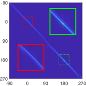 |
 |
 |
 |
|
| angle [deg] | angle [deg] | angle [deg] | angle [deg] |
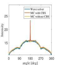
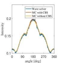
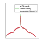
Coherent backscattering. Fig. 7 demonstrates coherent backscattering intensity, rendered using our algorithm with . We use a target of size , with a mean free path of , leading to an optical depth (that is, average number of scattering events) O.D.= 2. We simulate far-field sensors through all around the target, and near-field sensors located on a circle of diameter around the target. We compare the mean speckle intensity obtained from the electromagnetic solver with our Monte Carlo algorithm, considering forward and reversed paths, and with a simpler algorithm considering only forward paths derived in Appendix 9.5. For far-field sensors, we see that when the viewing direction approaches the inverse of the illumination direction, a narrow peak in brightness occurs, which is the manifestation of coherent backscattering. This peak is not predicted when using forward-only paths, but is indeed explained when using both forward and reversed paths. For near-field sensors, coherent backscattering is less pronounced and the two Monte Carlo algorithms are closer to each other.
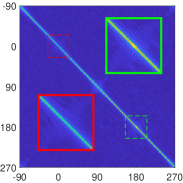
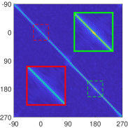
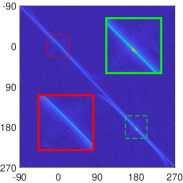
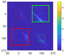
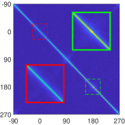
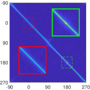
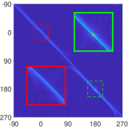
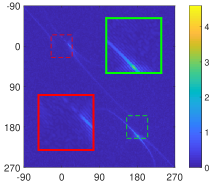
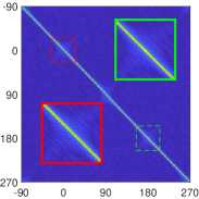
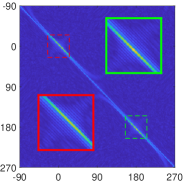
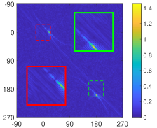
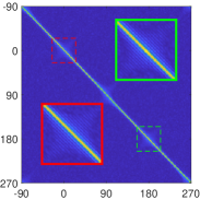
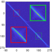
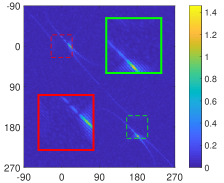
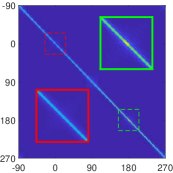
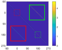
Memory effect. In Fig. 8, we show simulated covariance matrices for a target of size at O.D. and . We visualize covariance matrices of a target illuminated by two plane waves, measured at the far-field over viewing directions. In the covariance matrices, the memory effect is evident by the fact that, for small angles, the strongest correlation is obtained at a diagonal that is offset from the main diagonal, and the offset increases with the illumination angle difference. When the angle difference is large, the classical version of the memory effect no longer holds and the covariance is no longer a shifted diagonal. However, one can still observe some correlation along a curved set of viewing directions. To our best knowledge such correlations have not yet been explored, and provide an exciting direction of future research. In particular they may allow expanding the angular range of existing computational imaging techniques relying on the memory effect. We note also that, while the shape of the correlation curve is consistent, its exact value is a function of density, as seen from the two optical depths simulated in Fig. 8.
Runtime comparison. Overall, Figs. 7 and 8 illustrate that our Monte Carlo simulations provide useful and accurate predictions of speckle correlations, which is orders of magnitudes more efficiently than the approach based on the wave solver. To quantify the performance difference, in the small example of Fig. 8, simulating the covariance with the wave solver approach took 6 hours on a 50-core cluster, using the -diff solver (Thierry et al., 2015). By contrast, our Monte Carlo algorithm produced the same estimate in 45 minutes on a single core, using an unoptimized Matlab implementation. The difference in performance becomes even more drastic as the number of scatterers increases.
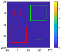
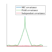
Field samples. We use Alg 2 to sample multiple speckle fields, as visualized in Fig. 1. Fig. 9 demonstrates their empirical covariance, showing good agreement with the covariance rendered directly by Alg. 1. We also compare with the simpler “electric field Monte Carlo” speckle rendering algorithm (Xu, 2004; Sawicki et al., 2008). This approach extends MC algorithms rendering intensities by using the length of the path as the phase. The main difference is that each sampled path is used to update only one sensor point, and therefore different illumination and viewing directions are updated independently. As a consequence, while this approach can accurately render intensity and even simulate coherent backscattering, it cannot reproduce spatial correlation. The target size and densities in Fig. 9 are equivalent to the setup of Fig. 8 at O.D. 2. It should be noted that (Xu, 2004; Sawicki et al., 2008) focus on modeling polarization correctly, while polarization is not addressed in our work.
6.2. Quantifying the memory effect of speckles
The memory effect of speckles is an active research area in optics, and has been a central property allowing researchers to develop techniques for seeing through scattering layers and around corners. Given its wide applicability, it is crucial to understand the range of illumination and viewing configurations for which we can indeed expect a high correlation between speckles.
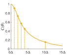
There have been multiple attempts (Osnabrugge et al., 2017; Berkovits and Feng, 1994; Fried, 1982) to derive closed-form formulas for speckle correlations. The complexity of multiple scattering means that this is only possible under various assumptions, which limit the approximation accuracy and the applicability of such formulas. The most commonly used result (Feng et al., 1988; Akkermans and Montambaux, 2007) is a formula derived under diffusion (i.e., high-order scattering) assumption,
| (39) |
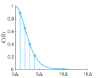
where is the angle between illumination and viewing directions, is the material thickness, and is the correlation between intensity images (rather than complex fields) and . The correlation of Eq. (39) decays to zero exponentially fast as soon as , hence the angular range at which the memory effect is valid is proportional to . In Sec. 6.2.3, we show that the Monte Carlo formulation can help understand this result.
The diffusion assumption used to derive Eq. (39) means that the formula applies only when the average number of scattering events on a path is large. However, empirical observations suggest that, in practice, the memory effect is valid through a much wider range. A few scenarios that have been observed to increase this range are (i) an average number of scattering events that is lower than the diffusive regime, (ii) absorption, (iii) forward scattering phase functions (Schott et al., 2015). Forward scattering is particularly important in practice, as tissue is known to be highly forward scattering and is usually described by an Henyey-Greenstein (HG) phase function with anisotropy parameter . Given the lack of analytic formulas and the practical importance of the problem, there have been multiple attempts to empirically measure the range of the memory effect of materials of interest in the lab (Schott et al., 2015; Yang et al., 2014; Mesradi et al., 2013).
Predicted correlation
…
…
…
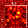
Indp. MC
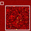
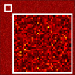
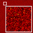
…
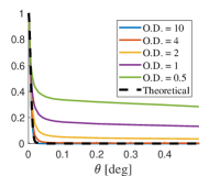
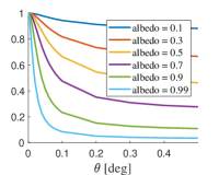
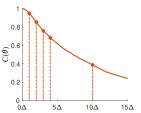
Our Monte Carlo algorithm can compute the expected correlations directly, without the need for approximations or lab measurements. Correlations are computed as a function of simple material parameters such as thickness, , and phase function. In Fig. 10, we show numerical calculations of the expected correlation as a function of angle . In Fig. 10b we use a forward scattering configuration, a sample of thickness at illumination wavelength , , isotropic phase function , and varying mean free path () values. For a high optical depth, the correlation computed by our algorithm agrees with the theoretical formula of Eq. (39), and as the optical depth decreases (mean free path increases) the range of the memory effect increases. In Fig. 10c we simulate a backscattering configuration for fixed , , , and varying albedo . As expected, the memory effect is stronger as absorption increases (albedo decreases).
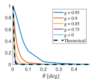
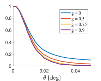
In Fig. 10d we keep the thickness and mean free path fixed to , and vary the anisotropy parameter of the phase function. As previous empirical observations report (Schott et al., 2015), increasing increases the transport mean free path, and thus the memory effect range expands. Finally, in Fig. 10e we investigate another common analytical approximation, the similarity theory (Wyman et al., 1989; Zhao et al., 2014), stating that scattering coefficient and phase functions satisfying should produce indistinguishable measurements. Using , , we set at a mean free path of (leading to ), and then vary and while maintaining the similarity relation. The graphs in Fig. 10e show that similarity theory is reasonably accurate, though low values have a somewhat heavier tail.
Our MC algorithm computes correlations of complex fields while Eq. (39) evaluates intensity correlations. Field covariances can be easily converted to intensity covariances using .
| (a) Source | (b) | (c) | |
|---|---|---|---|
| Illuminators | 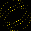 |
 |
 |
| Auto-corr | 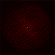 |
 |
 |
6.2.1. Sampling speckle images
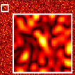
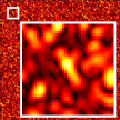
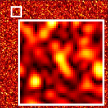
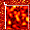
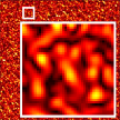
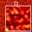
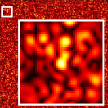
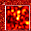
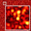
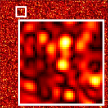
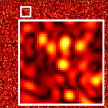
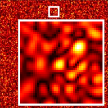
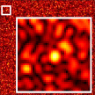
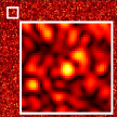
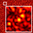
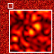
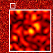
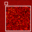
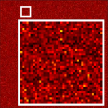
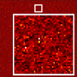
In Fig. 11 we use the sampling algorithm of Sec. 5.2 to sample speckle images as seen from a sensor at infinity over a viewing range of , when the illumination direction is shifting (from to , at intervals). As can be seen, these images reproduce the memory effect: For small changes in illumination angle the speckles appear as shifted versions of each other. When the illumination angle difference increases, the correlation decays. We show this simulation for a few anisotropy parameters and as illustrated in Fig. 10d, when the anisotropy increases the memory effect can be observed over a wider angular range. In the last row of Fig. 11 we show simulations using the electric field Monte Carlo approach (Xu, 2004; Sawicki et al., 2008), which updates different viewing and illumination directions independently. We observe that no joint speckle statistics are produced and the resulting images appear as independent noise.
6.2.2. Example application
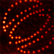
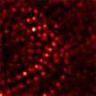
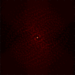
To demonstrate an application of speckle correlations, we reproduced the algorithm of Katz et al. (2014). This algorithm attempts to recover a set of incoherent light sources located behind a scattering layer. Remarkably, due to the memory effect, the auto-correlation of the speckle image should be equivalent to the auto-correlation of light sources positions. Thus, given the seemingly random speckle image, one can recover the position of light sources behind it by applying an iterative phase retrieval algorithm (Fienup, 1982). In Fig. 12 we show the result of this reconstruction applied on speckle images rendered with Algorithm 2. We use two of the materials in Fig. 10d, with anisotropy parameters . The hidden source is placed over an angular range of . As evaluated in Figs. 10d and 11, for this angular range the correlation for is high, but for we are already outside the memory effect range. Indeed the speckle auto-correlation at the bottom of Fig. 12b is almost equivalent to the source auto-correlation (Fig. 12a[bottom]), while the auto-correlation of speckles rendered with is darker due to the lower correlation (Fig. 12c[bottom]). As a result, phase retrieval with the speckles provides a good reconstruction of the original illuminator arrangement (Fig. 12b[top]). For (Fig. 12c[top]) only a cropped version of the illuminator pattern is recovered (along with background noise), as within this subset of illuminators the angular differences are smaller and the correlation is stronger. Experiments of this kind can be used to evaluate the applicability of the imaging technique of Katz et al. (2014) under different conditions, and to select optimal values for various parameters involved in an optical implementation of the technique.
6.2.3. Understanding the memory effect bounds
Before concluding this section, it is worth mentioning that the MC path integral formulation can provide an intuitive way to understand the memory effect range derived in Eq. (39). Consider two pairs of illumination and viewing directions s.t. , and consider a path starting at and ending at . Dropping attenuation, the phase contributed by this path to the correlation is
| (40) |
If tis complex number can have highly varying phases, than summing over multiple random paths averages to zero. The different paths interfere constructively only if the phase difference is negligible, roughly when . Intuitively, the average distance between an entrance point and an exit point on the target scales with the target depth, and it is reasonable to expect that is proportional to . This implies that the memory effect holds when , in agreement with Eq. (39).
7. Single-scattering approximation for covariance rendering
Before we conclude, we report an interesting property of speckle covariance, which can be used to accelerate its estimation under certain illumination and imaging conditions.
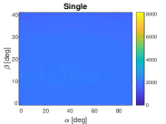
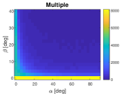
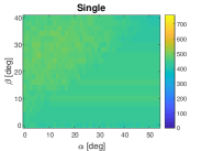
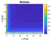
When simulating covariance using Monte Carlo rendering, we can separate contributions from paths of different numbers of bounces . For example, in Fig. 13, we show simulations for a cube volume of dimensions , and with O.D.=5, resulting in strong multiple scattering. We simulate the covariance for multiple pairs of illumination and imaging sets satisfying , for some target 3D vector . In each simulation, we decompose the rendered speckle covariance into two components, one accounting for contributions from paths that scattered once (), and another accounting for paths that scattered two or more times (). Within each rendered covariance matrix, the bottom left corner corresponds to rendering intensity.
 |
 |
 |
 |
| (a) | (b) | ||
We observe that, for the intensity case, the multiple-scattering component is dominant. By contrast, for cases where the difference between the two illumination or the two viewing directions is more than some small amount, the multiple-scattering component becomes negligible. This happens because, as the angle difference becomes large enough to bring us outside the range of the memory effect, multiply-scattered paths have complex contributions with randomly-varying phase, and therefore average to zero.
We conclude that, whenever the imaging and illumination conditions are such that we are outside the memory effect range, speckle covariance can be computed using only single scattering. This evaluation can be done in closed-form, avoiding the need for computationally-expensive Monte Carlo rendering. Namely, from a short derivation we can obtain the formula:
| (41) |
where .
The above discussion indicates that, whenever we are outside the memory effect range, we can accelerate the computation of speckle covariance by using the single-scattering approximation, without significant loss in accuracy. This is analogous to the use of the single-scattering approximation for accelerating intensity rendering (Sun et al., 2005; Walter et al., 2009), with an important difference: In the case of intensity the single-scattering approximation is valid only for very optically-thin volumes (Narasimhan et al., 2006). By contrast, in the case of covariance, the approximation can be accurate even for optically thick materials, given appropriate illumination and viewing conditions, making it more broadly applicable.
8. Discussion and Future Prospects
We conclude with a discussion of our contributions and possible future directions. We presented a path-integral formulation for the covariance of speckle fields generated by the interaction of coherent light with scattering volumes. Using this formulation, we derived two Monte Carlo rendering algorithms, one for directly estimating covariance, and another for directly generating speckle patterns. As we demonstrated in Section 6, our algorithms provide a unique combination of physical accuracy (closely matching solutions of the wave equation, reproducing known physical phenomena such as memory effect and coherent backscattering), computational efficiency (outperforming wave equation solvers by orders of magnitude), and parsimony (using only bulk macroscopic parameters of a volume, instead of requiring knowledge of its microscopic structure).
We note that our path-integral formulation for speckle covariance can potentially provide the foundation for deriving more sophisticated path sampling algorithms for rendering speckles, analogous to how the path-integral formulation for intensity spurred the invention of algorithms such as bidirectional path tracing and Metropolis light transport (Veach, 1997). In this context, we observe that our formulation is reciprocal, and therefore lends itself to the development of bidirectional path sampling algorithms.
In this paper we chose to focus on spatial speckle correlations. In doing so, we ignored another important class of second-order speckle statistics, temporal correlations resulting from moving scatterers. We hope that our results will motivate the development of analogous theoretical and simulation tools for temporal correlations. For instance, our rendering algorithms allow us to study the memory effect and related applications in cases where common assumptions (diffusion, Fokker-Planck limit) do not hold. Likewise, rendering algorithms for temporal correlations can allow extending related applications such as dynamic light scattering to cases where the common assumption of Brownian motion of scatterers is invalid (Duncan and Kirkpatrick, 2008).
The ability to render physically correct speckles can be highly beneficial for incorporating machine learning techniques into optics problems, where the collection of training data has been a major burden.
Last but not least, the findings of Sec. 7 suggest that measuring and rendering speckle covariance holds promise for inverse rendering applications. The fact that speckle covariance measurements are dominated by single scattering for a much larger class of materials than intensity measurements can potentially drastically simplify the volumetric inverse rendering problem, e.g., by potentially allowing us to replace the complex differentiable rendering of Gkioulekas et al. (2013; 2016) with simple analytic algorithms of Narasimhan et al. (2006). In addition to simplifying computation, it will be interesting to examine whether speckle covariance measurements can be used to relax previously reported ambiguities between scattering parameters (Wyman et al., 1989; Zhao et al., 2014).
References
- (1)
- Akkermans and Montambaux (2007) Eric Akkermans and Gilles Montambaux. 2007. Mesoscopic Physics of Electrons and Photons. Cambridge University Press.
- Batarseh et al. (2018) M. Batarseh, S. Sukhov, Z. Shen, H. Gemar, R. Rezvani, and A. Dogariu. 2018. Passive sensing around the corner using spatial coherence. Nature Communications.
- Baydoun et al. (2016) Ibrahim Baydoun, Diego Baresch, Romain Pierrat, and Arnaud Derode. 2016. Radiative transfer of acoustic waves in continuous complex media: Beyond the Helmholtz equation. Physical Review E.
- Bergmann et al. (2016) Stephan Bergmann, Mahsa Mohammadikaji, Stephan Irgenfried, Heinz Worn, Jürgen Beyerer, and Carsten Dachsbacher. 2016. A Phenomenological Approach to Integrating Gaussian Beam Properties and Speckle into a Physically-Based Renderer. In Vision, Modeling & Visualization.
- Berkovits and Feng (1994) Richard Berkovits and Shechao Feng. 1994. Correlations in coherent multiple scattering. Physics Reports (1994). https://doi.org/10.1016/0370-1573(94)90079-5
- Bertolotti et al. (2012) Jacopo Bertolotti, Elbert G. van Putten, Christian Blum, Ad Lagendijk, Willem L. Vos, and Allard P. Mosk. 2012. Non-invasive imaging through opaque scattering layers. Nature 491(7423), 232.
- Bitterli et al. (2018) Benedikt Bitterli, Srinath Ravichandran, Thomas Müller, Magnus Wrenninge, Jan Novák, Steve Marschner, and Wojciech Jarosz. 2018. A radiative transfer framework for non-exponential media. In SIGGRAPH Asia. ACM, 225.
- Boas and Yodh (1997) David A Boas and Arjun G. Yodh. 1997. Spatially varying dynamical properties of turbid media probed with diffusing temporal light correlation. J. Opt. Soc. Am. A.
- Bohren and Huffman (1983) Craig F. Bohren and Donald R. Huffman. 1983. Absorption and scattering of light by small particle. John Wiley & Sons.
- Cuypers et al. (2012) Tom Cuypers, Tom Haber, Philippe Bekaert, Se Baek Oh, and Ramesh Raskar. 2012. Reflectance Model for Diffraction. ACM Trans. Graph. 31, 5, Article 122, 11 pages. https://doi.org/10.1145/2231816.2231820
- d’Eon (2018a) Eugene d’Eon. 2018a. A Reciprocal Formulation of Non-Exponential Radiative Transfer. 2: Monte Carlo Estimation and Diffusion Approximation. arXiv preprint arXiv:1809.05881.
- d’Eon (2018b) Eugene d’Eon. 2018b. A reciprocal formulation of non-exponential radiative transfer with uncorrelated sources, detectors and boundaries. 1: Sketch and motivation. arXiv preprint arXiv:1803.03259.
- Dougherty et al. (1994) Ronald L. Dougherty, Bruce J. Ackerson, N.M. Reguigui, F. Dorri-Nowkoorani, and Ulf Nobbmann. 1994. Correlation transfer: Development and application. J. of Quantitative Spectroscopy and Radiative Transfer.
- Duncan and Kirkpatrick (2008) Donald D. Duncan and Sean J. Kirkpatrick. 2008. Can laser speckle flowmetry be made a quantitative tool? J. Opt. Soc. Am. A 25, 8, 2088–2094. https://doi.org/10.1364/JOSAA.25.002088
- Durduran et al. (2010) Turgut Durduran, Regine Choe, Wesley B. Baker, and Arjun G. Yodh. 2010. Diffuse optics for tissue monitoring and tomography. Reports on Progress in Physics.
- Dutré et al. (2006) Philip Dutré, Kavita Bala, and Philippe Bekaert. 2006. Advanced global illumination. AK Peters, Ltd.
- Erf (1978) Robert Erf. 1978. Speckle Metrology. Elsevier.
- Feng et al. (1988) Shechao Feng, Charles Kane, Patrick A Lee, and A Douglas Stone. 1988. Correlations and fluctuations of coherent wave transmission through disordered media. Physical review letters 61, 7, 834.
- Fienup (1982) James R. Fienup. 1982. Phase retrieval algorithms: a comparison. Appl. Opt. 21, 15, 2758–2769.
- Freund (1990) Isaac Freund. 1990. Looking through walls and around corners. Physica: Statistical Mechanics and its App.
- Freund and Eliyahu (1992) Isaac Freund and Danny Eliyahu. 1992. Surface correlations in multiple-scattering media. Phys Rev A (1992).
- Freund et al. (1988) Isaac Freund, Michael Rosenbluh, and Shechao. Feng. 1988. Memory Effects in Propagation of Optical Waves through Disordered Media. Phys. Rev. Lett. 61, 2328–2331. Issue 20. https://doi.org/10.1103/PhysRevLett.61.2328
- Fried (1982) David L. Fried. 1982. Anisoplanatism in adaptive optics. J. Opt. Soc. Am. 72, 1, 52–61. https://doi.org/10.1364/JOSA.72.000052
- Frisvad et al. (2007) Jeppe Revall Frisvad, Niels Jørgen Christensen, and Henrik Wann Jensen. 2007. Computing the scattering properties of participating media using Lorenz-Mie theory. SIGGRAPH.
- Gkioulekas et al. (2016) Ioannis Gkioulekas, Anat Levin, and Todd Zickler. 2016. An Evaluation of Computational Imaging Techniques for Heterogeneous Inverse Scattering.
- Gkioulekas et al. (2013) I. Gkioulekas, S. Zhao, K. Bala, T. Zickler, and A. Levin. 2013. Inverse Volume Rendering with Material Dictionaries. ACM Transactions on Graphics (Proc. ACM SIGGRAPH Asia) (2013).
- Goldburg (1999) W. I. Goldburg. 1999. Dynamic light scattering. American Journal of Physics (1999).
- Goodman (2007) Goodman. 2007. Speckle Phenomena in Optics: Theory and Applications. Roberts and Company Pub.
- Holodovski et al. (2016) Vadim Holodovski, Yoav Y. Schechner, Anat Levin, Aviad Levis, and Amit Aides. 2016. In-situ multi-view multi-scattering stochastic tomography. In ICCP.
- Ilyushin (2012) Y.A. Ilyushin. 2012. Coherent backscattering enhancement in highly anisotropically scattering media: Numerical solution. Journal of Quantitative Spectroscopy and Radiative Transfer (2012).
- Ishimaru (1999) Akira Ishimaru. 1999. Wave propagation and scattering in random media. Vol. 12. John Wiley & Sons.
- Jacquot and Fournier (2000) P. Jacquot and J. M. Fournier. 2000. Interferometry in Speckle Light. Springer.
- Jacquot and Rastogi (1979) Pierre Jacquot and Pramod K. Rastogi. 1979. Speckle motions induced by rigid-body movements in free-space geometry: an explicit investigation and extension to new cases. Appl. Opt. (1979).
- Jakobsen et al. (2012) M. L. Jakobsen, H. T. Yura, and S. G. Hanson. 2012. Spatial filtering velocimetry of objective speckles for measuring out-of-plane motion. Appl. Opt. (2012).
- Jarabo et al. (2018) Adrian Jarabo, Carlos Aliaga, and Diego Gutierrez. 2018. A Radiative Transfer Framework for Spatially-Correlated Materials. ACM Transactions on Graphics 37, 4 (2018).
- Katz et al. (2014) O. Katz, P. Heidmann, M. Fink, and S. Gigan. 2014. Non-invasive single-shot imaging through scattering layers and around corners via speckle correlation. Nat. Photonics (2014).
- Katz et al. (2012) O. Katz, E. Small, and Y. Silberberg. 2012. Looking around corners and through thin turbid layers in real time with scattered incoherent light. Nature (2012).
- Kaufmann (2011) Guillermo H. Kaufmann. 2011. Advances in Speckle Metrology and Related Techniques. Wiley.
- Levis et al. (2015) Aviad Levis, Yoav Y. Schechner, Amit Aides, and Anthony B. Davis. 2015. Airborne three-dimensional cloud tomography. In ICCV.
- Li and Genack (1994) J. H. Li and A. Z. Genack. 1994. Correlation in laser speckle. Phys. Rev. E 49 (May 1994), 4530–4533. Issue 5. https://doi.org/10.1103/PhysRevE.49.4530
- Lu et al. (2004) Qiang Lu, Xiaosong Gan, Min Gu, and Qingming Luo. 2004. Monte Carlo modeling of optical coherence tomography imaging through turbid media. Applied optics 43, 8 (2004), 1628–1637.
- Meng et al. (2015) Johannes Meng, Marios Papas, Ralf Habel, Carsten Dachsbacher, Steve Marschner, Markus H Gross, and Wojciech Jarosz. 2015. Multi-scale modeling and rendering of granular materials. ACM Trans. Graph. 34, 4 (2015), 49–1.
- Mesradi et al. (2013) M. Mesradi, A. Genoux, V. Cuplov, D. Abi Haidar, S. Jan, I. Buvat, and F. Pain. 2013. Experimental and analytical comparative study of optical coefficient of fresh and frozen rat tissues. Journal of Biomedical Optics (Nov. 2013). https://doi.org/10.1117/1.JBO.18.11.117010.
- Mishchenko et al. (2006) M.I. Mishchenko, L.D. Travis, and A.A. Lacis. 2006. Multiple scattering of light by particles: radiative transfer and coherent backscattering. Cambridge Univ Pr.
- Moon et al. (2007) Jonathan T Moon, Bruce Walter, and Stephen R Marschner. 2007. Rendering discrete random media using precomputed scattering solutions. In Proceedings of the 18th Eurographics conference on Rendering Techniques. Eurographics Association, 231–242.
- Mosk et al. (2013) Allard P. Mosk, Ad Lagendijk, Geoffroy Lerosey, and Mathias Fink. 2013. Controlling waves in space and time for imaging and focusing in complex media. Nat. Photonics (2013).
- Müller et al. (2016) Thomas Müller, Marios Papas, Markus H Gross, Wojciech Jarosz, and Jan Novák. 2016. Efficient rendering of heterogeneous polydisperse granular media. ACM Trans. Graph. 35, 6 (2016), 168–1.
- Narasimhan et al. (2006) S.G. Narasimhan, M. Gupta, C. Donner, R. Ramamoorthi, S.K. Nayar, and H.W. Jensen. 2006. Acquiring scattering properties of participating media by dilution. ACM Trans. Graph. 25, 3 (2006).
- Nixon et al. (2013) Micha Nixon, Ori Katz, Eran Small, Yaron Bromberg, Asher A. Friesem, Yaron Silberberg, and Nir Davidson. 2013. Real-time wavefront shaping through scattering media by all-optical feedback. Nat. Photonics (2013).
- Osnabrugge et al. (2017) Gerwin Osnabrugge, Roarke Horstmeyer, Ioannis N. Papadopoulos, Benjamin Judkewitz, and Ivo M. Vellekoop. 2017. Generalized optical memory effect. Optica (2017).
- Pan et al. (1995) Yingtian Pan, Reginald Birngruber, Jürgen Rosperich, and Ralf Engelhardt. 1995. Low-coherence optical tomography in turbid tissue: theoretical analysis. Applied optics 34, 28 (1995), 6564–6574.
- Pierrat et al. (2005) Romain Pierrat, Jean-Jacques Greffet, Rémi Carminati, and Rachid Elaloufi. 2005. Spatial coherence in strongly scattering media. J. Opt. Soc. Am. A 22, 11 (Nov 2005), 2329–2337.
- Pine et al. (1988) DJ Pine, DA Weitz, PM Chaikin, and E Herbolzheimer. 1988. Diffusing wave spectroscopy. Physical review letters 60, 12 (1988), 1134.
- Sawicki et al. (2008) John Sawicki, Nikolas Kastor, and Min Xu. 2008. Electric field Monte Carlo simulation of coherent backscattering of polarized light by a turbid medium containing Mie scatterers. Opt. Express 16, 8 (Apr 2008), 5728–5738.
- Schmitt and Knüttel (1997) Joseph M Schmitt and A Knüttel. 1997. Model of optical coherence tomography of heterogeneous tissue. JOSA A 14, 6 (1997), 1231–1242.
- Schott et al. (2015) Schott, Bertolotti, Léger, Bourdieu, and Gigan. 2015. Characterization of the angular memory effect of scattered light in biological tissues. Opt. Express (2015).
- Shen et al. (2017) Zhean Shen, Sergey Sukhov, and Aristide Dogariu. 2017. Monte Carlo method to model optical coherence propagation in random media. J. Opt. Soc. Am. A 34, 12 (Dec 2017), 2189–2193. https://doi.org/10.1364/JOSAA.34.002189
- Smith et al. (2017) Brandon M. Smith, Pratham Desai, Vishal Agarwal, and Mohit Gupta. 2017. CoLux: Multi-object 3D Micro-motion Analysis Using Speckle Imaging. ACM Trans. Graph. (2017).
- Stam (1999) J. Stam. 1999. Diffraction shaders. In SIGGRAPH.
- Sun et al. (2005) Bo Sun, Ravi Ramamoorthi, Srinivasa G Narasimhan, and Shree K Nayar. 2005. A practical analytic single scattering model for real time rendering. In ACM Transactions on Graphics (TOG), Vol. 24. ACM, 1040–1049.
- Thierry et al. (2015) B. Thierry, X. Antoine, C. Chniti, and H. Alzubaidi. 2015. -diff: An open-source Matlab toolbox for computing multiple scattering problems by disks. Computer Physics Communications 192 (2015), 348 – 362. https://doi.org/10.1016/j.cpc.2015.03.013
- Treeby and Cox. (2010) B. E. Treeby and B. T. Cox. 2010. k-Wave: MATLAB toolbox for the simulation and reconstruction of photoacoustic wave-fields,. J. Biomed. Opt. (2010).
- Twersky (1964) V. Twersky. 1964. On propagation in random media of discrete scatterers. Am. Math. Sot. Symp. Stochastic Processes in Mathematical Physics and Engineering, Vol. 16, p. 84 (1964).
- Veach (1997) E. Veach. 1997. Robust Monte Carlo methods for light transport simulation. Ph.D. Dissertation. PhD thesis, Stanford University.
- Vellekoop and Aegerter (2010) Ivo M. Vellekoop and Christof M. Aegerter. 2010. Scattered light fluorescence microscopy: imaging through turbid layers. Opt. Lett. 35, 8 (Apr 2010), 1245–1247. https://doi.org/10.1364/OL.35.001245
- Walter et al. (2009) Bruce Walter, Shuang Zhao, Nicolas Holzschuch, and Kavita Bala. 2009. Single scattering in refractive media with triangle mesh boundaries. In ACM Transactions on Graphics (TOG), Vol. 28. ACM, 92.
- Werner et al. (2017) Sebastian Werner, Zdravko Velinov, Wenzel Jakob, and Matthias B. Hullin. 2017. Scratch Iridescence: Wave-Optical Rendering of Diffractive Surface Structure. ACM SIGGRAPH Asia (2017).
- Wyman et al. (1989) Douglas R Wyman, Michael S Patterson, and Brian C Wilson. 1989. Similarity relations for anisotropic scattering in Monte Carlo simulations of deeply penetrating neutral particles. J. Comput. Phys. 81, 1 (1989), 137–150.
- Xu (2004) Min Xu. 2004. Electric field Monte Carlo simulation of polarized light propagation in turbid media. Opt. Express 12, 26 (Dec 2004), 6530–6539.
- Yan et al. (2018) Ling-Qi Yan, Miloš Hašan, Bruce Walter, Steve Marschner, and Ravi Ramamoorthi. 2018. Rendering specular microgeometry with wave optics. ACM Transactions on Graphics (TOG) 37, 4 (2018), 75.
- Yang et al. (2014) Xin Yang, Ye Pu, and Demetri Psaltis. 2014. Imaging blood cells through scattering biological tissue using speckle scanning microscopy. Opt. Express 22, 3 (Feb 2014), 3405–3413. https://doi.org/10.1364/OE.22.003405
- Yee (1966) K. Yee. 1966. Numerical solution of initial boundary value problems involving Maxwell’s equations in isotropic media. EEE Trans. on Antennas and Propagation (1966).
- Yeh et al. (2013) Hengchin Yeh, Ravish Mehra, Zhimin Ren, Lakulish Antani, Dinesh Manocha, and Ming Lin. 2013. Wave-ray Coupling for Interactive Sound Propagation in Large Complex Scenes. ACM Trans. Graph. (2013).
- Zhao et al. (2014) Shuang Zhao, Ravi Ramamoorthi, and Kavita Bala. 2014. High-order similarity relations in radiative transfer. ACM Transactions on Graphics (TOG) 33, 4 (2014), 104.
9. Appendix
9.1. Bulk parameters with multiple particle types
For the simplicity of the exposition our algorithm was derived in the main paper assuming particles of a single type. Here we show that with small adjustments we can handle any mixture of particle types. We index the particle type with a subscript . We assume we are given as input a possibly spatially varying distribution of the density of each type of particle, denoted by . For each particle type we denote its scattering and absorption cross sections by its radius by , and its normalized amplitude function by .
We start by defining the bulk parameters that summarize the density and scattering amplitude of all particle types using some mean statistics. Then we revisit some equations in the main text that should be readjusted when more than one type of particles is involved.
First let us denote by the mean number of particles from type in a unit volume. For spherical particles, this can be computed by dividing the density by the volume of a particle with radius
| (42) |
To account for the fact that we work with normalized amplitude and phase functions, we define the scattering and absorption coefficients as the expected energy scattered/absorbed from a unit sized volume, namely the expected number of particles in a unit volume times the cross section
| (43) |
where is the attenuation coefficient of the leading medium. extinction coefficient is defined via .
We define the bulk outer product of amplitude functions as
| (44) |
and as a special case of the above, define the phase function as .
We will also define a bulk amplitude function as
| (45) |
However, in most cases the product of scattering amplitude at two angles is defined via Eq. (44) and not as , since two paths scattering at a single point also scatter at a particle of the same type.
To see how this quantity folds into the speckle covariance derivation, let us start with the speckle mean.
9.2. The speckle mean
Eq. (18) for the mean of all paths from a near field point to a point (near field or far field) should be conditioned on the type of particle at , and should be expressed as:
| (46) |
where we scale by because, while is defined using the normalized scattering amplitude function, the total energy scattered by a particle is a function of its size.
If either the source or the sensor are at the near field (i.e. points rather than directions), the mean of all speckle fields given a source at and a sensor at is a special case of Eq. (46), omitting the term representing the direction change
| (47) |
When both source and sensor are at the far field, we need to integrate Eq. (46) through all possible scattering points in space.
Claim 1.
The mean of all paths from a far field source to a far field sensor is
| (48) |
As this integral involves the phase of the paths from to and from to , it reduces quickly if paths with multiple phases are involved and it is non zero mostly for the forward scattering direction .
Proof.
To justify this equation let us divide the space of all paths from to to sets , defined as the set of all paths whose first scattering event happens at point . To average the contribution of all paths in this group, let us assume that we know point includes a particle of type . Note that the path phase from the beginning at to is given by . From to there are many paths, since they all start at the same point we can use Eq. (46) implying that their average contribution is . Thus the contribution of all paths in the set integrates to
| (49) |
To get from here to Eq. (48) we need to weight Eq. (49) by the expected number of particles in a unit volume.
9.3. Integrals in path space
Having derived the mean let us move to the covariance. Our goal here is to derive expectations of path contributions and justify Eq. (22). For this we introduce the notation
| (50) |
with defined in Eq. (44), and where is the equivalent of with an amplitude function of particle type :
| (51) |
The term should replace all terms of the form in the definition of the speckle covariance, and the resulting changes to the MC process are summarised in Alg 3. Effectively this is encoding the fact that when two paths scatter at the same particle they scatter at a particle from the same type, so the same should apply to both.
To analyze the path contributions we will divide the space of all path pairs from to to sets defined by the nodes they have in common. Let denote a set of nodes and two possibly different permutations of these nodes. We look at the set of all paths that share exactly the nodes in in the orders:
| (52) |
where any occurrence of in Eq. (52) can be replaced with any sequence of nodes, as long as they are different from each other. With this definition we can divide the space of all paths to disjoint sets. Below we argue that the throughput contribution from each set averages to the volumetric throughput contribution of the direct paths .
In the following we use the notation , for the nodes before and after in the permuted sequence , and similarly for , , .
Claim 2.
| (53) |
with
| (54) |
Proof.
Let us start by drawing an independent set of nodes . According to the target density, the probability for these particles is the last term of Eq. (53), . For each position we draw a particle type . Given the type of all particles on the paths we decompose the path probabilities.
Let denote the set of all disjoint paths from to and from to , and let denote the end direction of (i.e. the direction at which the last segment is entering or ). While the only constraint on is that they are disjoint, we will make the approximation that they are independent. (Mishchenko et al., 2006) shows that the error introduced by this approximation is where is the expected number of particles in the medium. Thus we can write
| (55) |
Using Eq. (18):
| (56) | |||||
Since all paths in the set integrate to the direct path, we know that the end directions when entering are , . Given the end direction of the first segment we can apply Eq. (18) to the second segment, and in a similar way, to all successive segments:
| (57) |
Concatenating Eqs. (56) and (57) assuming the particle position and type is given, and permuting the order of nodes accordingly, provides
| (58) |
If we now sum Eq. (58) for all all possible assignment of particle types and consider also the probability of sampling the nodes themselves, we get Eq. (53).
9.4. Path permutations
As mentioned in Sec. 4.2, Claim 2 significantly simplifies the path sampling algorithm, since the fact that all paths collapse to their joint nodes allows us to largely reduce the sampling space. However, Claim 2 does not imply that the joint paths appear at the same order. Since every particle instantiation that contains a set of nodes contains all its permutations, paths pairs tracing the same set of nodes at different orders are not independent. If we want to derive a MC algorithm which accounts for all permutations, we can use the update rule defined below.
Let be a set of nodes sampled according to some path probability . Let be a set of permutations on entries, and let (for ) denote a permuted version of connected to the start and end nodes
| (59) |
To account for all permutations, we redefine from Eq. (31) as
| (60) |
and the next event estimation should update the correlation by
| (61) |
where the numerator sums over all path pairs in all permutations, and in the denominator we divide by the probability of sampling these paths, since for every path we add all permutations, there are multiple ways to sample it. In practice the update rules of Eq. (34) is a special case of Eq. (61) when the permutation set was taken to include the identity and reversed permutations.
For materials whose optical depth is low and the average number of scattering events in a path is not high, we could implement the accurate update rule of Eq. (61). For large path lengths , the factor is computationally prohibiting.
As mentioned in the main text, our simulations show that considering the forward and reversed permutations only is accurate enough, as it agrees very well with the covariances produced by the exact wave solver.
 |
 |
 |
 |
|
 |
 |
 |
 |
|
| (a) Forward | (b) Reversed | (c) Permutation 1 | (d) Permutation 2 |
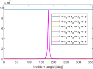
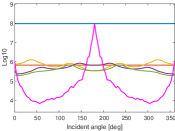
The reason most permutations can be ignored is that the phase of the path throughput is equivalent to the path length and for permutations that do not trace the nodes in the same order the segment lengths are different (Fig. 5b), hence we are summing complex numbers with different phases that quickly integrate to zero. To see this we considered paths of 3 nodes , which is the smallest path length with non trivial permutations. In Fig. 14 we used , fixed the nodes while varying the third node over a area. We evaluated the path throughput contributions for various permutations on 3 nodes. When is the identity permutations and have the same length, hence is always a positive number. If is the reversed permutation leading to the path we get a fixed phase only for the backscattering direction . For other directions one can see in Fig. 14b lower row that perturbing the position of changes the phase, hence it is clear that by averaging the pairwise path throughput over all positions of averages to zero
| (62) |
For all other permutations, there is not even a single configuration of illumination and viewing directions leading to a fixed phase, and as can be seen in Fig. 14c, varying the position of one of the nodes locally quickly changes the phase, hence averaging different path contributions over a local window integrates to zero. There are some rare path selections leading to a locally stationary phase, as can be seen in Fig. 14d. However, the probability of selecting such paths is low, and therefore the contribution to the overall covariance is negligible. In Fig. 15 we numerically evaluated the integral of all 6 permutations of 3 numbers when varying two of the scatterers positions through a 2D square
| (63) |
One can see that except of the forward and reversed permutations the throughput of all permutations integrates to a contribution that is about two order of magnitude lower than the forward contribution.
9.5. The correlation transfer equation
MC algorithms evaluating scattering intensity were historically derived in computer graphics based on the radiative transfer equation (RTE), which is an integral equation expressing the intensity at one point using the intensity at other points in space. A MC is then defined as a recursive evaluation of the RTE. One of the main results in the speckle correlation literature is an analogues correlation transfer equation (CTE) (Ishimaru, 1999; Twersky, 1964). This is an integral equation that expresses the correlation through the light field intensity at other points in space. In contrary to the way this was developed in computer graphics, textbooks like (Mishchenko et al., 2006) derive the CTE and RTE starting from electro-magnatic equations and express their solution as a summation of path-pairs contributions.
The CTE (Ishimaru, 1999; Twersky, 1964) considers speckles at different spatial points under the same illumination direction, and express their second order moments. In our notations is the speckle covariance that relates to the second order moments as: . The CTE states that:
| (64) |
Where is the “light field” as used traditionally in computer graphics, namely the intensity arriving point from direction .
The important observation made by the CTE is that to compute correlations between the fields at sensor points , we need to integrate only intensity from other space points, and there is no need to memorize any other correlations. The intensity at other space points is weighted by the volumetric throughput , namely the probability and phase of making a “single scattering” step from to and . For the case the covariance reduces to intensity and indeed Eq. (64) reduces to the integral version of the RTE assuming zero emission inside the target. The is basically the attenuation and phase function part of the RTE, and the term is the attenuation of the direct source.
It is not hard to show that for the case a forward-only MC version summarized in Algorithm 3 is basically a recursive evaluation of this CTE integral. This variant is derived by approximating the covariance as
| (65) |
Rather than as
| (66) |
The derivation of the CTE e.g. in (Mishchenko et al., 2006) follows an expression of the solution to the wave equation as a sum of path contributions as we have presented in the previous sections. Making the simplifying assumption that only forward path pairs need to be considered they reorganize all the paths in the summation in a more compact recursive formula which is essentially the CTE, or the RTE in the case. The fact that only forward paths are considered is an inherent assumption necessary for the compactness of the CTE, namely that one needs to memorize only the last node on a path and the rest of its history does not matter. However, this is also its main drawback, as it does not allow it to explain physical phenomena such as coherent backscattering, which is an interference effect generated by the full path and not only by the last event. Due to this problem we chose to derive our covariance rendering directly from a path space formulation and not through an integral equation.
9.6. Sampling a speckle image with multiple particle types
Before concluding we note that sampling a speckle image as defined in Alg. 2 should also adjust when multiple types of particles are available. The covariance in the multiple type case is expressed as:
| (67) |
With
| (68) |
Therefore, for every node sample we should also sample a particle type . We summarize the changes in Alg. 4.
