Non-Gaussian Geostatistical Modeling using (skew) t Processes

Abstract

We propose a new model for regression and dependence analysis when addressing spatial data with possibly heavy tails and an asymmetric marginal distribution. We first propose a stationary process with $t$ marginals obtained through scale mixing of a Gaussian process with an inverse square root process with Gamma marginals. We then generalize this construction by considering a skew-Gaussian process, thus obtaining a process with skew-t marginal distributions. For the proposed (skew) $t$ process we study the second-order and geometrical properties and in the $t$ case, we provide analytic expressions for the bivariate distribution. In an extensive simulation study, we investigate the use of the weighted pairwise likelihood as a method of estimation for the $t$ process. Moreover we compare the performance of the optimal linear predictor of the $t$ process versus the optimal Gaussian predictor. Finally, the effectiveness of our methodology is illustrated by analyzing a georeferenced dataset on maximum temperatures in Australia.

Keywords: Heavy-tailed processes; Hypergeometric functions; Multivariate skew-normal distribution; Scale mixing; Pairwise likelihood.

1 Introduction

The geostatistical approach models data coming from a limited number of monitoring stations as a partial realization from a spatial stochastic process (or random field) defined on the continuum space. Gaussian stochastic processes are among the most popular tools for analyzing spatial data because a mean structure and a valid covariance function completely characterized the associated finite dimensional distribution. Additionally, optimal prediction at an unobserved site depends on the knowledge of the covariance function of the process. Unfortunately, in many geostatistical applications, including climatology, oceanography, the environment and the study of natural resources, the Gaussian framework is unrealistic because the observed data have specific features such as negative or positive asymmetry and/or heavy tails.

The focus of this work is on non-Gaussian models for stochastic processes that vary continuously in the euclidean space, even if the proposed methodology can be easily extended to the space-time framework or to the spherical space. In particular, we aim to accommodate heavier tails than the ones induced by Gaussian processes and wish to allow possible asymmetry. In recent years, different approaches have been proposed in order to analyze these kind of data. Transformation of Gaussian (trans-Gaussian) processes is a general method to model non-Gaussian spatial data obtained by applying some nonlinear transformations to the original data (De Oliveira et al., 1997; Allcroft and Glasbey, 2003; De Oliveira, 2006). Then statistical analyses can be carried out on the transformed data using any techniques available for Gaussian processes. However, it can be difficult to find an adequate nonlinear transformation and some appealing properties of the latent Gaussian process may not be inherited by the transformed process. A flexible trans-Gaussian process based on the Tukey $g-h$ distribution has been proposed in Xua and Genton (2017).

Wallin and Bolin (2015) proposed non-Gaussian processes derived from stochastic partial differential equations to model non-Gaussian spatial data. However this approach is restricted to the Matérn covariance model with integer smoothness parameter and its statistical properties are much less understood than those of the Gaussian process.

The copula framework (Joe, 2014) has been adapted in the spatial context in order to account for possible deviations from the Gaussian distribution. Even though which copula model to use for a given analysis is not generally known a priori, the copula based on the multivariate Gaussian distribution has gained a general consensus (Kazianka and Pilz, 2010; Masarotto and Varin, 2012; Gräler, 2014) since the definition of the multivariate dependence relies again on the specification of the correlation function. However, Gaussian copula could be too restrictive in some cases since it expresses a symmetrical and elliptical dependence.

Convolution of Gaussian and non-Gaussian processes is an appealing strategy for modeling spatial data with skewness. For instance, Zhang and El-Shaarawi (2010) proposed a Gaussian-Half Gaussian convolution in order to construct a process with marginal distributions of the skew-Gaussian type (Azzalini and Capitanio, 2014). Zareifard et al. (2018) developed bayesian inference for the estimation of a process with asymmetric marginal distributions obtained through convolution of Gaussian and Log-Gaussian processes. Mahmoudian (2017) proposed a skew-Gaussian process using the skew-model proposed in Sahu et al. (2003). The resulting process is not mean-square continuous and as a consequence it is not a suitable model for data exhibiting smooth behavior of the realization.

On the other hand, mixing of Gaussian and non-Gaussian processes is a useful strategy for modeling spatial data with heavy tails. For instance, Palacios and Steel (2006) and Zareifard and Khaledi (2013) proposed a (skew) Gaussian-Log-Gaussian scale mixing approach in order to accommodate the presence of possible outliers for spatial data.

The $t$ distribution is a parametric model that is able to accommodate flexible tail behavior, thus providing robust estimates against extreme data and it has been studied extensively in recent years (Arellano-Valle and Bolfarine, 1995; Lange et al., 1989; Fonseca et al., 2008; Ferrari and Arellano-Valle, 1996; Arellano-Valle et al., 2012). Stochastic processes with marginal $t$ distributions have been introduced in Røislien and Omre (2006), Ma (2009), Ma (2010a) and DeBastiani et al. (2015), but as outlined in Genton and Zhang (2012), these models are not be identifiable when only a single realization is available (which is typically the case for spatial data).

In this paper, we propose a process with marginal $t$ distributions obtained though scale mixing of a standard Gaussian process with an inverse square root process with Gamma marginals. The latter is obtained through a rescaled sum of independent copies of a standard squared Gaussian process. Although this can be viewed as a natural way to define a $t$ process, the associated second-order, geometrical properties and bivariate distribution are somewhat unknown to the best of our knowledge. Some results can be found in Heyde and Leonenko (2005) and Finlay and Seneta (2006). We study the second-order and geometrical properties of the $t$ process and we provide analytic expressions for the correlation and the bivariate distribution. It turns out that both depend on special functions, particularly the Gauss hypergeometric and Appell function of the fourth type (Gradshteyn and Ryzhik, 2007). In addition, the bivariate distribution is not of elliptical type.

We then focus on processes with asymmetric marginal distributions and heavy tails. We first review the skew Gaussian process proposed in Zhang and El-Shaarawi (2010). For this process we provide an explicit expression of the finite dimensional distribution generalizing previous results in Alegría et al. (2017). We then propose a process with marginal distribution of the skew-$t$ type (Azzalini and Capitanio, 2014) obtained through scale mixing of a skew-Gaussian with an inverse square root process with Gamma marginals.

Our proposals for the $t$ and skew-$t$ processes have two main features. First, they allow removal of any problem of identifiability (Genton and Zhang, 2012), and as a consequence, all the parameters can be estimated using one realization of the process. Second, the $t$ and skew-$t$ processes inherit some of the geometrical properties of the underlying Gaussian process. This implies that the mean-square continuity and differentiability of the $t$ and skew-$t$ processes can be modeled using suitable parametric correlation models as the Matérn model (Matèrn, 1986) or the Generalized Wendland model (Gneiting, 2002; Bevilacqua et al., 2019).

For the $t$ process estimation we propose the method of weighted pairwise likelihood (Lindsay, 1988; Varin et al., 2011; Bevilacqua and Gaetan, 2015) exploiting the bivariate distribution given in Theorem 2.3. In an extensive simulation study we investigate the performance of the weighted pairwise likelihood ($wpl$) method under different scenarios including when the degrees of freedom are supposed to be unknown. We also study the performance of the $wpl$ estimation by assuming a Gaussian process in the estimation step with correlation function equal to the correlation function of the $t$ process. It turns out that the Gaussian misspecified $wpl$ (see Gouriéroux et al. (2017) with the references therein) leads to a less efficient estimator, as expected. However, the method has some computational benefits.

Additionally, we compare the performance of the optimal linear predictor of the $t$ process with the optimal predictor of the Gaussian process. Finally we apply the proposed methodology by analyzing a real data set of maximum temperature in Australia where, in this case, we consider a $t$ process defined on a portion of the sphere (used as an approximation of the planet Earth) and use a correlation model depending on the great-circle distance (Gneiting, 2013).

The methodology considered in this paper is implemented in the R package GeoModels (Bevilacqua and Morales-Oñate, 2018). The remainder of the paper is organized as follows. In Section 2 we introduce the $t$ process, study the second-order and geometrical properties and provide an analytic expression for the bivariate distribution. In Section 3, we first study the finite dimensional distribution of the skew Gaussian process, and then we study the second-order properties of the skew-$t$ process. In Section 4, we present a simulation study in order to investigate the performance of the (misspecified) $wpl$ method when estimating the $t$ process and the performance of the associated optimal linear predictor versus the optimal Gaussian predictor. In Section 5, we analyze a real data set of maximum temperature in Australia. Finally, in Section 6, we give some conclusions. All the proofs has been deferred to the Appendix.

2 A stochastic process with $t$ marginal distribution

For the rest of the paper, given a process $Q=\{Q(\bm{s}),\bm{s}\in A\}$ with $\operatorname{E}(Q(\bm{s}))=\mu(\bm{s})$ and $Var(Q(\bm{s}))=\sigma^{2}$, we denote by $\rho_{Q}(\bm{h})=Corr(Q(\bm{s}_{i}),Q(\bm{s}_{j}))$ its correlation function, where $\bm{h}=\bm{s}_{i}-\bm{s}_{j}$ is the lag separation vector. For any set of distinct points $(\bm{s}_{1},\ldots,\bm{s}_{n})^{T}$, $n\in\mathcal{N}$, we denote by $\bm{Q}_{ij}=(Q(\bm{s}_{i}),Q(\bm{s}_{j}))^{T}$, $i\neq j$, the bivariate random vector and by $\bm{Q}=(Q(\bm{s}_{1}),\ldots,Q(\bm{s}_{n}))^{T}$ the multivariate random vector. Moreover, we denote with $f_{Q(\bm{s})}$ and $F_{Q(\bm{s})}$ the marginal probability density function (pdf) and cumulative distribution function (cdf) of $Q(\bm{s})$ respectively, with $f_{\bm{Q}_{ij}}$ the pdf of $\bm{Q}_{ij}$ and with $f_{\bm{Q}}$ the pdf of $\bm{Q}$. Finally, we denote with $Q^{*}$ the standardized weakly stationary process, $i.e.$, $Q^{*}(\bm{s}):=(Q(\bm{s})-\mu(\bm{s}))/\sigma$.

As outlined in Palacios and Steel (2006), given a positive process $M=\{M(\bm{s}),\bm{s}\in A\}$ and an independent standard Gaussian process $G^{*}=\{G^{*}(\bm{s}),\bm{s}\in A\}$, a general class of non-Gaussian processes with marginal heavy tails can be obtained as scale mixture of $G^{*}$, $i.e.$ $\mu(\bm{s})+\sigma M(\bm{s})^{-\frac{1}{2}}G^{*}(\bm{s})$, where $\mu(\bm{s})$ is the location dependent mean and $\sigma>0$ is a scale parameter. A typical parametric specification for the mean is given by $\mu(\bm{s})=X(\bm{s})^{T}\bm{\beta}$ where $X(\bm{s})\in\mathbb{R}^{k}$ is a vector of covariates and $\bm{\beta}\in\mathbb{R}^{k}$ but other types of parametric or nonparametric functions can be considered.

Henceforth, we call $G^{*}$ the ‘parent’ process and with some abuse of notation we set $\rho(\bm{h}):=\rho_{G^{*}}(\bm{h})$ and $G:=G^{*}$. Our proposal considers a mixing process $W_{\nu}=\{W_{\nu}(\bm{s}),\bm{s}\in A\}$ with marginal distribution $\Gamma(\nu/2,\nu/2)$ defined as $W_{\nu}(\bm{s}):=\sum_{i=1}^{\nu}G_{i}(\bm{s})^{2}/\nu$ where $G_{i}$, $i=1,\ldots\nu$ are independent copies of $G$ with $\operatorname{E}(W_{\nu}(\bm{s}))=1$, $Var(W_{\nu}(\bm{s}))=2/\nu$ and $\rho_{W_{\nu}}(\bm{h})=\rho^{2}(\bm{h})$ (Bevilacqua et al., 2018). If we consider a process $Y^{*}_{\nu}=\{Y^{*}_{\nu}(\bm{s}),\bm{s}\in A\}$ defined as

$$Y^{*}_{\nu}(\bm{s}):=W_{\nu}(\bm{s})^{-\frac{1}{2}}G(\bm{s}),$$ (2.1)

then, by construction, $Y^{*}_{\nu}$ has the marginal $t$ distribution with $\nu$ degrees of freedom with pdf given by:

$$f_{Y^{*}_{\nu}(\bm{s})}(y;\nu)=\frac{\Gamma\left(\frac{\nu+1}{2}\right)}{\sqrt{\pi\nu}\Gamma\left(\frac{\nu}{2}\right)}\left(1+\frac{y^{2}}{\nu}\right)^{-\frac{(\nu+1)}{2}}.$$ (2.2)

Then, we define the location-scale transformation process $Y_{\nu}=\{Y_{\nu}(\bm{s}),\bm{s}\in A\}$ as:

$$Y_{\nu}(\bm{s}):=\mu(\bm{s})+\sigma Y^{*}_{\nu}(\bm{s})$$ (2.3)

with $\operatorname{E}(Y_{\nu}(\bm{s}))=\mu(\bm{s})$ and $Var(Y_{\nu}(\bm{s}))=\sigma^{2}\nu/(\nu-2)$, $\nu>2$.

Remark 1: A possible drawback for the Gamma process $W_{\nu}$ is that it is a limited model due to the restrictions to the half-integers for the shape parameter. Actually, in some special cases, it can assume any positive value greater than zero. This feature is intimately related to the infinite divisibility of the squared Gaussian process $G^{2}=\{G^{2}(\bm{s}),\bm{s}\in A\}$ as shown in Krishnaiah and Rao (1961). Characterization of the infinite divisibility of $G^{2}$ has been studied in Vere-Jones (1997), Bapat (1989), Griffiths (1970) and Eisenbaum and Kaspi (2006). In particular Bapat (1989) provides a characterization based on $\Omega$, the correlation matrix associated with $\rho(\bm{h})$. Specifically, $\nu>0$ if and only if there exists a matrix $S_{n}$ such that $S_{n}\Omega^{-1}S_{n}$ is an $M$-matrix (Plemmons, 1977), where $S_{n}$ is a signature matrix, $i.e$., a diagonal matrix of size $n$ with entries either $1$ or $-1$. This condition is satisfied, for instance, by a stationary Gaussian random process $G$ defined on $A=\mathbb{R}$ with an exponential correlation function. The $t$ process $Y^{*}_{\nu}$ inherits this feature with the additional restriction $\nu>2$. This implies that $Y^{*}_{\nu}$ is well defined for $\nu=3,4,\ldots$ and for $\nu>2$ under non-infinite divisibility of $G^{2}$.

Remark 2: The finite dimensional distribution of $Y^{*}_{\nu}$ is unknown to the best of our knowledge, but in principle, it can be derived by mixing the multivariate density associated with $W^{-\frac{1}{2}}_{\nu}$ with the multivariate standard Gaussian density. The multivariate Gamma density $f_{\bm{W}_{\nu}}$ was first discussed by Krishnamoorthy and Parthasarathy (1951) and its properties have been studied by different authors (Royen, 2004; Marcus, 2014). In the bivariate case, Vere-Jones (1967) showed that the bivariate Gamma distribution is infinite divisible, $i.e.$ $\nu>0$ in (A.2), irrespective of the correlation function. Note that this is consistent with the characterization given in Bapat (1989) since, given an arbitrary bivariate correlation matrix $\Omega$, there exists a matrix $S_{2}$ such that $S_{2}\Omega^{-1}S_{2}$ is a $M$-matrix. In Theorem 2.3 we provide the bivariate distribution of $Y^{*}_{\nu}$

Note that, both $W_{\nu}$ and $G$ in (2.3) are obtained through independent copies of the ‘parent’ Gaussian process with correlation $\rho(\bm{h})$. For this reason, henceforth, in some cases, we will call $Y^{*}_{\nu}$ a standard $t$ process with underlying correlation $\rho(\bm{h})$.

In what follows, we make use of the Gauss hypergeometric function defined by (Gradshteyn and Ryzhik, 2007):

$${}_{2}F_{1}(a,b,c;x)=\sum\limits_{k=0}^{\infty}\frac{(a)_{k}(b)_{k}}{(c)_{k}}\frac{x^{k}}{k!},\;\;\;$$ (2.4)

with $(s)_{k}=\Gamma(s+k)/\Gamma(s)$ for $k\in\mathbb{N}\cup\{0\}$ being the Pochhammer symbol and we consider the restrictions $a>0$, $b>0$, $c>0$ and $x\geq 0$. If $c>a+b$ the radius of convergence of (2.4) is $0\leq x\leq 1$ and, in particular (2.4) is convergent at $x=1$ trough the identity:

$${}_{2}F_{1}\left(a,b;c;1\right)=\frac{\Gamma(c)\Gamma(c-a-b)}{\Gamma(c-a)\Gamma(c-b)}.$$ (2.5)

We also consider the Appell hypergeometric function of the fourth type (Gradshteyn and Ryzhik, 2007) defined as:

$$F_{4}(a,b;c,c^{\prime};w,z)=\sum\limits_{k=0}^{\infty}\sum\limits_{m=0}^{\infty}\frac{(a)_{k+m}(b)_{k+m}w^{k}z^{m}}{k!m!(c)_{k}(c^{\prime})_{m}},\;\;\;\;|\sqrt{w}|+|\sqrt{z}|<1.$$

The following Theorem gives an analytic expression for $\rho_{Y^{*}_{\nu}}(\bm{h})$ in terms of the Gauss hypergeometric function.

Theorem 2.1.

Let $Y^{*}_{\nu}$ be a standardized $t$ process with underlying correlation $\rho(\bm{h})$. Then:

$$\rho_{Y^{*}_{\nu}}(\bm{h})=\frac{(\nu-2)\Gamma^{2}\left(\frac{\nu-1}{2}\right)}{2\Gamma^{2}\left(\frac{\nu}{2}\right)}\left[{}_{2}F_{1}\left(\frac{1}{2},\frac{1}{2};\frac{\nu}{2};\rho^{2}(\bm{h})\right)\rho(\bm{h})\right].$$ (2.6)

The following Theorem depicts some features of the $t$ process. It turns out that nice properties such as stationarity, mean-square continuity and degrees of mean-square differentiability can be inherited from the ‘parent’ Gaussian process $G$. Further, the $t$ process has long-range dependence when the ‘parent’ Gaussian process has long-range dependence and this can be achieved when the correlation has some specific features. For instance, the generalized Cauchy (Gneiting and Schlather, 2004; Lim and Teo, 2009) and Dagum (Berg et al., 2008) correlation models can lead to a Gaussian process with long range dependence. Finally, an appealing and intuitive feature is that the correlation of $Y^{*}_{\nu}$ approaches the correlation of $G$ when $\nu\to\infty$.

Theorem 2.2.

Let $Y^{*}_{\nu}$, $\nu>2$ be a standardized $t$ process with underlying correlation $\rho(\bm{h})$. Then:

1. $Y^{*}_{\nu}$ is also weakly stationary;

2. $Y^{*}_{\nu}$ is mean-square continuous if and only if $G$ is mean-square continuous;

3. Let $G$ $m$-times mean-square differentiable, for $m=0,1,\ldots$

   • If $\nu>2(2m+1)$ then $Y^{*}_{\nu}$ is $m$-times mean-square differentiable;

   • If $\nu\leq 2(2m+1)$ then $Y^{*}_{\nu}$ is $(m-k)$-times mean-square differentiable if $2(2(m-k)+1)<\nu\leq 2(2(m-k)+3)$, for $k=1,\ldots,m$.

4. $Y^{*}_{\nu}$ is a long-range dependent process if and only if $G$ is a long-range dependent process

5. $\rho_{Y^{*}_{\nu}}(\bm{h})\leq\rho(\bm{h})$ and $\lim\limits_{\nu\to\infty}\rho_{Y^{*}_{\nu}}(\bm{h})=\rho(\bm{h})$.

One implication of Theorem (2.2) point c) is that the process $Y^{*}_{\nu}$ inherits the mean square differentiability of $G$ under the condition $\nu>2(2m+1)$. Otherwise, the mean square differentiability depends on $\nu$. For instance, if $G$ is one time mean square differentiable then $Y^{*}_{\nu}$ can be zero or one time differentiable depending if $\nu>6$ or not.

Remark 3: A simplified version of the $t$ process in Equation (2.1), can be obtained assuming $W_{\nu}(\bm{s}_{i})\perp W_{\nu}(\bm{s}_{j}),i\neq j$. Under this assumption, $Y^{*}_{\nu}$ is still a process with $t$ marginal distribution but, in this case, the geometrical properties are not inherited from the ‘parent’ Gaussian process $G$. In particular, it can be shown that the resulting correlation function exhibits a discontinuity at the origin and, as a consequence, the process is not mean-square continuous. A not mean-square continuous version of the $t$ process in Equation (2.1), can be obtained by introducing a nugget effect, i.e., a discontinuity of $\rho_{Y^{*}_{\nu}}(\bm{h})$ at the origin. This can be easily achieved by replacing $\rho(\bm{h})$ in (2.6) with $\rho^{*}(\bm{h})=1$ if $\bm{h}=\bm{0}$ and $\rho^{*}(\bm{h})=(1-\tau^{2})\rho(\bm{h})$ otherwise, where $0\leq\tau^{2}<1$ represents the underlying nugget effect.

Since the $t$ process inherits some of the geometrical properties of the ‘parent’ Gaussian process, the choice of the covariance function is crucial. Two flexible isotropic models that allow parametrizing in a continuous fashion the mean square differentiability of a Gaussian process and its sample paths are as follows:

1. the Matérn correlation function (Matèrn, 1986)

   $${\cal M}_{\alpha,\psi}(\bm{h})=\frac{2^{1-\psi}}{\Gamma(\psi)}\left({||\bm{h}||}/{\alpha}\right)^{\psi}{\cal K}_{\psi}\left({||\bm{h}||}/{\alpha}\right),$$ (2.7)

   where ${\cal K}_{\psi}$ is a modified Bessel function of the second kind of order $\psi$. Here, $\alpha>0$ and $\psi>0$ guarantee the positive definiteness of the model in any dimension.

2. the Generalized Wendland correlation function (Gneiting, 2002), defined for $\psi>0$ as:

   $${\cal GW}_{\alpha,\psi,\delta}(\bm{h}):=\begin{cases}\frac{\int_{||\bm{h}||/\alpha}^{1}u\left(u^{2}-(||\bm{h}||/\alpha)^{2}\right)^{\psi-1}\left(1-u\right)^{\delta}du}{{\operatorname{B}(2\psi,\delta+1)}}&||\bm{h}||<\alpha\\ 0&\text{otherwise}\end{cases},$$ (2.8)

   and for $\psi=0$ as:

   $${\cal GW}_{\alpha,0,\delta}(\bm{h}):=\begin{cases}\left(1-||\bm{h}||/\alpha\right)^{\delta}&||\bm{h}||<\alpha\\ 0&\text{otherwise}\end{cases}.$$ (2.9)

   Here $\operatorname{B}(\cdot,\cdot)$ is the Beta function and $\alpha>0$, $\delta\geq(d+1)/2+\psi$ guarantee the positive definiteness of the model in $\mathbb{R}^{d}$.

In particular for a positive integer $k$, the sample paths of a Gaussian process are $k$ times differentiable if and only if $\psi>k$ in the Matérn case (Stein, 1999) and if and only if $\psi>k-1/2$ in the Generalized Wendland case (Bevilacqua et al., 2019). Additionally, the Generalized Wendland correlation is compactly supported, an interesting feature from computational point of view (Furrer et al., 2013), which is inherited by the $t$ process since $\rho(\bm{h})=0$ implies $\rho_{Y^{*}_{\nu}}(\bm{h})=0$.

In order to illustrate some geometric features of the $t$ process, we first compare the correlation functions of the Gaussian and $t$ processes using an underlying Matérn model. In Figure 1 (left part) we compare $\rho_{Y^{*}_{\nu}}(\bm{h})$ when $\nu=3,7$ with the correlation of the ‘parent’ Gaussian process $\rho(\bm{h})={\cal M}_{1.5,\alpha^{*}}(\bm{h})$ where $\alpha^{*}$ is chosen such that the practical range is $0.2$. It is apparent that when increasing the degrees of freedom $\rho_{Y^{*}_{\nu}}(\bm{h})$ approaches $\rho(\bm{h})$ and that the smoothness at the origin of $\rho_{Y^{*}_{\nu}}(\bm{h})$ is inherited by the smoothness of the Gaussian correlation $\rho(\bm{h})$ when $\nu=7$ and if $\nu=3$ then $\rho_{Y^{*}_{\nu}}(\bm{h})$ is not differentiable at the origin. On the right side of Figure (1) we compare a kernel nonparametric density estimation of a realization of $G$ and a realization of $Y^{*}_{7}$ (approximately 10000 location sites in the unit square) using $\rho(\bm{h})={\cal M}_{1.5,\alpha^{*}}(\bm{h})$.

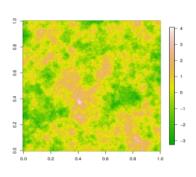
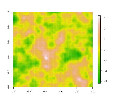
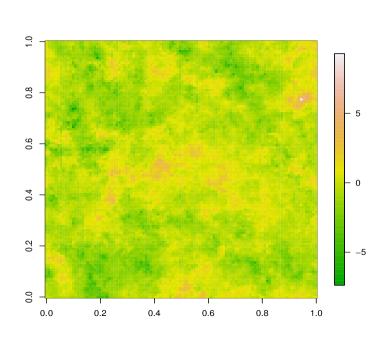
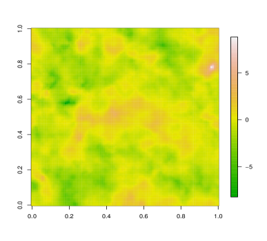
In Figure 2 (a) and (b), we compare, from left to right, two realizations of $G$ with $\rho(\bm{h})={\cal M}_{0.5,\alpha^{*}}(\bm{h})$ and $\rho(\bm{h})={\cal M}_{1.5,\alpha^{*}}(\bm{h})$ where $\alpha^{*}$ is chosen such that the practical range is $0.2$. In this case, the sample paths of $G$ are zero and one times differentiable. From the bottom part of Figure 2 (c) and (d) it can be appreciated that this feature is inherited by the associated realizations of $Y^{*}_{7}$.

Figure 1: Left part: comparison of $\rho_{Y^{*}_{\nu}}(\bm{h})$, $\nu=3,7$ with the correlation $\rho(\bm{h})$ of the ‘parent’ Gaussian process $G$ when $\rho(\bm{h})={\cal M}_{1.5,\alpha^{*}}(\bm{h})$ with $\alpha^{*}$ such that the practical range is $0.2$. Right part: a comparison of a nonparametric kernel density estimation of realizations from $G$ and from the $t$ process $Y^{*}_{7}$.

(a)	(b)
(c)	(d)

Figure 2: Upper part: two realizations of the ‘parent’ Gaussian process $G$ on $[0,1]^{2}$ with (a) $\rho(\bm{h})={\cal M}_{0.5,\alpha^{*}}(\bm{h})$ and (b) $\rho(\bm{h})={\cal M}_{1.5,\alpha^{*}}(\bm{h})$ (from left to right) with $\alpha^{*}$ such that the practical range is approximatively $0.2$. Bottom part: (c) and (d) associated realizations of the $t$ process $Y^{*}_{7}$.

We now consider the bivariate random vector associated with $Y^{*}_{\nu}$ defined by:

$$\bm{Y}^{*}_{\nu;ij}=\bm{W}^{-\frac{1}{2}}_{\nu;ij}\circ\bm{G}_{ij}$$

where $\circ$ denotes the Schur product vector. The following Theorem gives the pdf of $\bm{Y}^{*}_{\nu;ij}$ in terms of the Appell function $F_{4}$. It can be viewed as a generalization of the generalized bivariate $t$ distribution proposed in Miller (1968).

Theorem 2.3.

Let $Y^{*}_{\nu}$, $\nu>2$ be a standard $t$ process with underlying correlation $\rho(\bm{h})$. Then:

$$f_{\bm{Y}^{*}_{\nu;ij}}(y_{i},y_{j}) =\frac{\nu^{\nu}l_{ij}^{-\frac{(\nu+1)}{2}}\Gamma^{2}\left(\frac{\nu+1}{2}\right)}{\pi\Gamma^{2}\left(\frac{\nu}{2}\right)(1-\rho^{2}(\bm{h}))^{-(\nu+1)/2}}F_{4}\left(\frac{\nu+1}{2},\frac{\nu+1}{2},\frac{1}{2},\frac{\nu}{2};\frac{\rho^{2}(\bm{h})y_{i}^{2}y_{j}^{2}}{l_{ij}},\frac{\nu^{2}\rho^{2}(\bm{h})}{l_{ij}}\right)$$

$$+\frac{\rho(\bm{h})y_{i}y_{j}\nu^{\nu+2}l_{ij}^{-\frac{\nu}{2}-1}}{2\pi(1-\rho^{2}(\bm{h}))^{-\frac{(\nu+1)}{2}}}F_{4}\left(\frac{\nu}{2}+1,\frac{\nu}{2}+1,\frac{3}{2},\frac{\nu}{2};\frac{\rho^{2}(\bm{h})y_{i}^{2}y_{j}^{2}}{l_{ij}},\frac{\nu^{2}\rho^{2}(\bm{h})}{l_{ij}}\right)$$ (2.10)

where $l_{ij}=[(y_{i}^{2}+\nu)(y_{j}^{2}+\nu)]$.

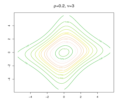
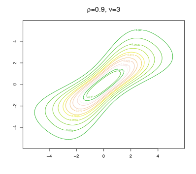
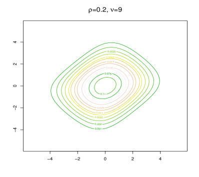
Figure 3: Contour plots of the bivariate $t$ distribution (2.3) when $\rho(\bm{h})=0.2,0.9$ and $\nu=3,9$.

Remark 4: Note that $f_{\bm{Y}^{*}_{\nu;ij}}(y_{i},y_{j})$ is defined for $\nu>2$ irrespectively of the correlation function since it is obtained from a bivariate Gamma distribution (see Remark 2). Moreover, when $\rho(\bm{h})=0$, according to (4.3) and using the identity ${}_{2}F_{1}(a,b;c^{\prime};0)=1$, we obtain $F_{4}(a,b;c,c^{\prime};0,0)=1$, and as a consequence, $f_{\bm{Y}^{*}_{\nu;ij}}(y_{i},y_{j})$ can be written as the product of two independent $t$ random variables with $\nu$ degrees of freedom. Thus, zero pairwise correlation implies pairwise independence, as in the Gaussian case. Figure (3) show the contour plots of (2.3) when $\nu=3,9$ and $\rho(\bm{h})=0.2,0.9$. It turns out that the bivariate $t$ distribution is not elliptical and when increasing $\nu$ the contour plots tend towards an elliptical form. Finally, the bivariate density of the process $Y_{\nu}$ is easily obtained from (2.3):

$$f_{\bm{Y}_{\nu;ij}}(y_{i},y_{j})=\frac{1}{\sigma^{2}}f_{\bm{Y}^{*}_{\nu;ij}}\left(\frac{y_{i}-\mu_{i}}{\sigma},\frac{y_{j}-\mu_{j}}{\sigma}\right).$$ (2.11)

3 A stochastic process with skew-t marginal distribution

In this section we first review the skew-Gaussian process proposed in Zhang and El-Shaarawi (2010). For this process, we provide an explicit expression for the finite dimensional distribution generalizing previous results in Alegría et al. (2017). Then, using this skew-Gaussian process, we propose a generalization of the $t$ process $Y_{\nu}$ obtaining a new process with marginal distribution of the skew-t type (Azzalini and Capitanio, 2014).

Following Zhang and El-Shaarawi (2010) a general construction for a process with asymmetric marginal distribution is given by:

$$U_{\eta}(\bm{s}):=g(\bm{s})+\eta|X_{1}(\bm{s})|+\omega X_{2}(\bm{s}),\;\;\;\bm{s}\in A\subset\mathbb{R}^{d}$$ (3.1)

where $\eta\in\mathbb{R}$, $\omega>0$ and $X_{i}$ $i=1,2$ are two independents copies of a process $X=\{X(\bm{s}),\bm{s}\in A\}$ with symmetric marginals. The parameters $\eta$ and $\omega$ allow modeling the asymmetry and variance of the process simultaneously.

Zhang and El-Shaarawi (2010) studied the second-order properties of $U_{\eta}$ when $X\equiv G$. In this case, $U_{\eta}$ has skew Gaussian marginal distributions (Azzalini and Capitanio, 2014) with pdf given by:

$$f_{U_{\eta}(\bm{s})}(u)=\frac{2}{(\eta^{2}+\omega^{2})^{1/2}}\phi\left(\frac{(u-g(\bm{s}))}{(\eta^{2}+\omega^{2})^{1/2}}\right)\Phi\left(\frac{\eta(u-g(\bm{s}))}{\omega(\eta^{2}+\omega^{2})^{1/2}}\right)$$ (3.2)

with $\operatorname{E}(U_{\eta}(\bm{s}))=g(\bm{s})+\eta(2/\pi)^{1/2}$, $Var(U_{\eta}(\bm{s}))=\omega^{2}+\eta^{2}(1-2/\pi)$ and with correlation function given:

$$\rho_{U_{\eta}}(\bm{h})=\frac{2\eta^{2}}{\pi\omega^{2}+\eta^{2}(\pi-2)}\left((1-\rho^{2}(\bm{h}))^{1/2}+\rho(\bm{h})\arcsin(\rho(\bm{h}))-1\right)+\frac{\omega^{2}\rho(\bm{h})}{\omega^{2}+\eta^{2}(1-2/\pi)}.$$ (3.3)

The following theorem generalizes the results in Alegría et al. (2017) and gives an explicit closed-form expression for the pdf of the random vector $\bm{U}_{\eta}$.

Theorem 3.1.

Let $U_{\eta}(\bm{s})=g(\bm{s})+\eta|X_{1}(\bm{s})|+\omega X_{2}(\bm{s})$ where $X_{i}$ $i=1,2$ are two independent copies of $G$ the ‘parent’ Gaussian process. Then:

$$f_{\bm{U}_{\eta}}(\bm{u})=2\sum\limits_{l=1}^{2^{n-1}}\phi_{n}(\bm{u}-\bm{\alpha};\bm{A}_{l})\Phi_{n}(\bm{c}_{l};\bm{0},\bm{B}_{l})$$ (3.4)

where

$$\bm{A}_{l} =\omega^{2}\Omega+\eta^{2}\Omega_{l}$$

$$\bm{c}_{l} =\eta\Omega_{l}(\omega^{2}\Omega+\eta^{2}\Omega_{l})^{-1}(\bm{u}-\bm{\alpha})$$

$$\bm{B}_{l} =\Omega_{l}-\eta^{2}\Omega_{l}(\omega^{2}\Omega+\eta^{2}\Omega_{l})^{-1}\Omega_{l}$$

$$\bm{\alpha} =[g(\bm{s}_{i})]_{i=1}^{n}$$

and the $\Omega_{l}$’s are correlation matrices that depend on the correlation matrix $\Omega$.

Some comments are in order. First, note that $f_{\bm{U}}$ can be viewed as a generalization of the multivariate skew-Gaussian distribution proposed in Azzalini and Dalla-Valle (1996). Second, using Theorem (3.1), it can be easily shown that the consistency conditions given in Mahmoudian (2018) are satisfied. Third, it is apparent that likelihood-based methods for the skew-Gaussian process are impractical from computational point of view even for a relatively small dataset.

To obtain a process with skew-$t$ marginal distributions (Azzalini and Capitanio, 2014), we replace the process $G$ in (2.3) with the process $U_{\eta}$. Specifically, we consider a process $S_{\nu,\eta}=\{S_{\nu,\eta}(\bm{s}),\bm{s}\in A\}$ defined as

$$S_{\nu,\eta}(\bm{s}):=\mu(\bm{s})+\sigma W_{\nu}(\bm{s})^{-\frac{1}{2}}U_{\eta}(\bm{s})$$ (3.5)

where $W_{\nu}$ and $U_{\eta}$ are supposed to be independent. In (3.1) we assume $g(\bm{s})=0$ and $\eta^{2}+\omega^{2}=1$. The pdf of the marginal distribution of $S^{*}_{\nu,\eta}$ is given by:

$$f_{S^{*}_{\nu,\eta}(\bm{s})}(g)=2f_{Y^{*}_{\nu}(\bm{s})}(g;\nu)F_{Y^{*}_{\nu}(\bm{s})}\left(\eta g\sqrt{\frac{\nu+1}{\nu+g^{2}}};\nu+1\right)$$ (3.6)

with $\operatorname{E}(S^{*}_{\nu,\eta}(\bm{s}))=\frac{\sqrt{\nu}\Gamma\left(\frac{\nu-1}{2}\right)\eta}{\sqrt{\pi}\Gamma\left(\frac{\nu}{2}\right)}$, and $Var(S^{*}_{\nu,\eta}(\bm{s}))=\left[\frac{\nu}{\nu-2}-\frac{\nu\Gamma^{2}\left(\frac{\nu-1}{2}\right)\eta^{2}}{\pi\Gamma^{2}\left(\frac{\nu}{2}\right)}\right]$.

If $\eta=0$, (3.6) reduces to a marginal $t$ density given in (2.2) and if $\nu\to\infty$, (3.6) converges to a skew-normal distribution. Moreover, coupling (2.6) and (3.3) the correlation function of the skew-$t$ process is given by:

$$\rho_{S^{*}_{\nu,\eta}}(\bm{h}) =a(\nu,\eta)\left[{}_{2}F_{1}\left(\frac{1}{2},\frac{1}{2};\frac{\nu}{2};\rho^{2}(\bm{h})\right)\left\{(1+\eta^{2}(1-\frac{2}{\pi}))\rho_{U_{\eta}}(\bm{h})+\frac{2\eta^{2}}{\pi}\right\}-\frac{2\eta^{2}}{\pi}\right],$$ (3.7)

where $a(\nu,\eta)=\frac{\pi(\nu-2)\Gamma^{2}\left(\frac{\nu-1}{2}\right)}{2\left[\pi\Gamma^{2}\left(\frac{\nu}{2}\right)(1+\eta^{2})-\eta^{2}(\nu-2)\Gamma^{2}\left(\frac{\nu-1}{2}\right)\right]}$. Note that $\rho_{S^{*}_{\nu,\eta}}(\bm{h})=\rho_{S^{*}_{\nu,-\eta}}(\bm{h})$ that is, as in the skew-Gaussian process $U_{\eta}$, the correlation is invariant with respect to positive or negative asymmetry and using similar arguments of Theorem 2.2 point e), it can be shown that $\lim\limits_{\nu\to\infty}\rho_{S^{*}_{\nu,\eta}}(\bm{h})=\rho_{U_{\eta}}(\bm{h})$.

Finally, following the steps of the proof of Theorem 2.2, it can be shown that properties $a)$, $b)$, $c)$ and $d)$ in Theorem 2.2 are true for the skew-t process $S^{*}_{\nu,\eta}$.

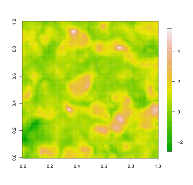
Figure 4, left part, compares $\rho_{S^{*}_{7,0.9}}(\bm{h})$ and $\rho_{S^{*}_{7,0}}(\bm{h})=\rho_{Y^{*}_{7}}(\bm{h})$ with the underlying correlation $\rho(\bm{h})={\cal GW}_{0.3,1,5}(\bm{h})$. The right part shows a realization of $S^{*}_{7,0.9}$.

Figure 4: From left to right: a) comparison between $\rho_{S^{*}_{7,0.9}}(\bm{h})$, $\rho_{S^{*}_{7,0}}(\bm{h})=\rho_{Y^{*}_{7}}(\bm{h})$ and the underlying correlation $\rho(\bm{h})={\cal GW}_{0.3,1,5}(\bm{h})$; b) a realization from $S^{*}_{7,0.9}(\bm{s})$.

4 Numerical examples

In this Section we analyze the performance of the $wpl$ method when estimating the $t$ process assuming $\nu$ known or unknown. Following Remark 1 in Section 2, we consider the cases when $\nu>2$ and $\nu=3,4,\ldots$. In the latter case, we give a practical solution for fixing the degrees of freedom parameter to a positive integer value through a two-step estimation.

We also compare the performance of the $wpl$ using the bivariate $t$ distribution (2.3) with a misspecified Gaussian standard and weighted pairwise likelihood. Finally, we compare the performance of the optimal linear predictor of the $t$ process using (2.6) versus the optimal predictor of the Gaussian process.

4.1 Weighted pairwise likelihood estimation

Let $(y_{1},\ldots,y_{n})^{T}$ be a realization of the $t$ random process $Y_{\nu}$ defined in equation (2.3) observed at distinct spatial locations $\bm{s}_{1},\ldots,\bm{s}_{n}$, $\bm{s}_{i}\in A$ and let $\bm{\theta}=(\bm{\beta}^{T},\nu,\sigma^{2},\bm{\alpha}^{T})$ be the vector of unknown parameters where $\bm{\alpha}$ is the vector parameter associated with the underlying correlation model. The method of $wpl$, (Lindsay, 1988; Varin et al., 2011) combines the bivariate distributions of all possible distinct pairs of observations. The pairwise likelihood function is given by

$$\operatorname{pl}(\bm{\theta}):=\sum_{i=1}^{n-1}\sum_{j=i+1}^{n}\log(f_{\bm{Y}_{\nu;ij}}(y_{i},y_{j};\bm{\theta})){c_{ij}}$$ (4.1)

where $f_{\bm{Y}_{\nu;ij}}(y_{i},y_{j};\bm{\theta})$ is the bivariate density in (2.11) and $c_{ij}$ is a nonnegative suitable weight. The choice of cut-off weights, namely

$$c_{ij}=\begin{cases}1&\|\bm{s}_{i}-\bm{s}_{j}\|\leq d_{ij}\\ 0&\text{otherwise}\end{cases},$$ (4.2)

for a positive value of $d_{ij}$, can be motivated by its simplicity and by observing that the dependence between observations that are distant is weak. Therefore, the use of all pairs may skew the information confined in pairs of near observations (Bevilacqua and Gaetan, 2015; Joe and Lee, 2009). The maximum $wpl$ estimator is given by

$$\widehat{\bm{\theta}}:=\operatorname{argmax}_{\bm{\theta}}\,\operatorname{pl}(\bm{\theta})$$

and, arguing as in Bevilacqua et al. (2012) and Bevilacqua and Gaetan (2015), under some mixing conditions of the $t$ process, it can be shown that, under increasing domain asymptotics, $\widehat{\bm{\theta}}$ is consistent and asymptotically Gaussian with the asymptotic covariance matrix given by $\mathcal{G}^{-1}_{n}(\bm{\theta})$ the inverse of the Godambe information $\mathcal{G}_{n}(\bm{\theta}):=\mathcal{H}_{n}(\bm{\theta})\mathcal{J}_{n}(\bm{\theta})^{-1}\mathcal{H}_{n}(\bm{\theta}),$ where $\mathcal{H}_{n}(\bm{\theta}):=\operatorname{E}[-\nabla^{2}\operatorname{pl}(\bm{\theta})]$ and $\mathcal{J}_{n}(\bm{\theta}):={\mbox{Var}}[\nabla\operatorname{pl}(\bm{\theta})]$. Standard error estimation can be obtained considering the square root diagonal elements of $\mathcal{G}^{-1}_{n}(\widehat{\bm{\theta}})$. Moreover, model selection can be performed by considering two information criterion, defined as

$$\mbox{PLIC}:=-2\operatorname{pl}(\hat{\bm{\theta}})+2\mathrm{tr}(\mathcal{H}_{n}(\hat{\bm{\theta}})\mathcal{G}^{-1}_{n}(\hat{\bm{\theta}})),\quad\mbox{BLIC}:=-2\operatorname{pl}(\hat{\bm{\theta}})+log(n)\mathrm{tr}(\mathcal{H}_{n}(\hat{\bm{\theta}})\mathcal{G}^{-1}_{n}(\hat{\bm{\theta}}))$$

which are composite likelihood version of the Akaike information criterion (AIC) and Bayesian information criterion (BIC) respectively (Varin and Vidoni, 2005; Gao and Song, 2010). Note that, the computation of standard errors, PLIC and BLIC require evaluation of the matrices $\mathcal{H}_{n}(\hat{\bm{\theta}})$ and $\mathcal{J}_{n}(\hat{\bm{\theta}})$. However, the evaluation of $\mathcal{J}_{n}(\hat{\bm{\theta}})$ is computationally unfeasible for large datasets and in this case subsampling techniques can be used in order to estimate $\mathcal{J}_{n}(\bm{\theta})$ as in Bevilacqua et al. (2012) and Heagerty and Lele (1998). A straightforward and more robust alternative is parametric bootstrap estimation of $\mathcal{G}^{-1}_{n}(\bm{\theta})$ (Bai et al., 2014). We adopt the second strategy in Section 5.

4.2 Performance of the weighted pairwise likelihood estimation

Following DiCiccio and Monti (2011) and Arellano-Valle and Azzalini (2013) we consider a reparametrization for the $t$ process by using the inverse of degrees of freedom, $\lambda=1/\nu$. In the standard i.i.d case this kind of parametrization has proven effective for solving some problems associated with the singularity of the Fisher information matrix associated to the original parametrization. Here we consider two possible scenarios i.e. a $t$ process observed on a subset of $\mathbb{R}$ and $\mathbb{R}^{2}$.

1. We consider points $s_{i}\in A=[0,1]$, $i=1,\ldots,N$ and an exponential correlation function for the ‘parent’ Gaussian process. Then, according to Remark 1 in section 2, the $t$ process is well-defined for $0<\lambda<1/2$ and in this specific case all the parameters can be jointly estimated. We simulate, using Cholesky decomposition, $500$ realizations of a $t$ process observed on a regular transect $s_{1}=0$, $s_{2}=0.002,\ldots,s_{501}=1$. We consider two mean regression parameters, that is, $\mu(s_{i})=\beta_{0}+\beta_{1}u(s_{i})$ with $\beta_{0}=0.5$, $\beta_{1}=-0.25$ where $u(s_{i})$ is a realization from a $U(0,1)$. Then we set $\lambda=1/\nu$, $\nu=3,6,9$ and $\sigma^{2}=1$.

   As correlation model we consider $\rho(h)={\cal M}_{\alpha,0.5}(h)=e^{-|h|/\alpha}$ with $\alpha=0.1/3$ and in the $wpl$ estimation we consider a cut-off weight function with $d_{ij}=0.002$. Table 1 shows the bias and mean square error (MSE) associated with $\lambda$, $\beta_{0}$, $\beta_{1}$, $\alpha$ and $\sigma^{2}$.

2. We consider points $\bm{s}_{i}\in A=[0,1]^{2}$, $i=1,\ldots,N$. Specifically, we simulate, using Cholesky decomposition, $500$ realizations of a $t$ process observed at $N=500$ spatial location sites uniformly distributed in the unit square. Regression, variance and (inverse of) degrees of freedom parameters have been set as in the first scenario. As an isotropic parametric correlation model, $\rho(\bm{h})={\cal GW}_{\alpha,0,4}(\bm{h})$ with $\alpha=0.2$ is considered. In the $wpl$ estimation we consider a cut-off weight function with $d_{ij}=0.05$ and for each simulation we estimate with $wpl$, assuming the degrees of freedom are fixed and known.

   We also consider the more realistic case when the (inverse of) degrees of freedom are supposed to be unknown. Recall that from Remark 1, $\nu$ must be fixed to a positive integer $\nu=3,4,\ldots$ in order to guarantee the existence of the $t$ process. A brute force approach considers different $wpl$ estimates using a fixed $\lambda=1/\nu$, $\nu=3,4,\ldots$. and then simply keeps the estimate with the best $PLIC$ or $BLIC$. We propose a computationally easier approach by considering a two-step method. In the first step, we estimate all the parameters including $0<\lambda<1/2$ maximizing the $wpl$ function. This is possible since the bivariate $t$ distribution is well defined for $0<\lambda<1/2$ (see Remark 4). In the second step $\nu$ is fixed equal to the rounded value of $1/\widehat{\lambda}_{1}$ where $\widehat{\lambda}_{1}$ is the estimation at first step. (If at the first step, the estimation of $1/\widehat{\lambda}_{1}$ is lower than $2.5$, then it is rounded to $3$). Table 2 shows the bias and MSE associated with $\beta_{0}$, $\beta_{1}$, $\alpha$ and $\sigma^{2}$ when estimating with $wpl$, assuming (the inverse of) degrees of freedom 1) known and fixed, and 2) unknown and fixed using a two-step estimation and Figure 5 shows the boxplots of the $wpl$ estimates for the case 1) and 2).

As a general comment, the distribution of the estimates are quite symmetric, numerically stable and with very few outliers for the three scenarios. In Scenario 1, the MSE of $\lambda=1/\nu$ slightly decreases when increasing $\nu$. Moreover, in Table 2, it can be appreciated that only the estimation of $\sigma^{2}$ is affected when considering a two step estimation. Specifically, the MSE of $\sigma^{2}$ slightly increases with respect to the one-step estimation, $i.e.$, when the degrees of freedom are supposed to be known.

$\lambda$	$1/3$		$1/6$		$1/9$
	Bias	MSE	Bias	MSE	Bias	MSE
$\hat{\lambda}$	$-0.01022$	$0.00321$	$-0.01033$	$0.00215$	$-0.00924$	$0.00172$
$\hat{\beta}_{0}$	$-0.01466$	$0.06585$	$-0.00559$	$0.06154$	$0.00028$	$0.06532$
$\hat{\beta}_{1}$	$-0.00099$	$0.00062$	$-0.00232$	$0.00049$	$-0.00193$	$0.00049$
$\hat{\alpha}$	$-0.00213$	$0.0006$	$-0.00278$	$0.0007$	$-0.00189$	$0.0008$
$\hat{\sigma}^{2}$	$-0.01064$	$0.07493$	$-0.05502$	$0.06902$	$-0.02677$	$0.07052$

Table 1: Bias and MSE when estimating with $wpl$ the $t$ process with $\lambda=1/\nu$, $\nu=3,6,9$ and exponential correlation function (Scenario 1).

$\lambda$	$1/3$				$1/6$				$1/9$
	1		2		1		2		1		2
	Bias	MSE	Bias	MSE	Bias	MSE	Bias	MSE	Bias	MSE	Bias	MSE
$\hat{\beta}_{0}$	$-0.00024$	$0.01261$	$-0.00037$	$0.01271$	$0.00712$	$0.01139$	$0.00712$	$0.01135$	$0.00638$	$0.01153$	$0.00646$	$0.0115$
$\hat{\beta}_{1}$	$-0.00702$	$0.00874$	$-0.00721$	$0.00881$	$0.00419$	$0.00697$	$0.00419$	$0.00696$	$-0.00089$	$0.00685$	$-0.00098$	$0.00694$
$\hat{\alpha}$	$-0.00233$	$0.00058$	$-0.00352$	$0.00058$	$-0.00115$	$0.00059$	$-0.00143$	$0.00061$	$-0.00425$	$0.00056$	$-0.0048$	$0.00058$
$\hat{\sigma}^{2}$	$-0.00971$	$0.01341$	$0.01768$	$0.01745$	$-0.01056$	$0.01142$	$-0.00461$	$0.01694$	$-0.01049$	$0.01148$	$-0.00015$	$0.01657$

Table 2: Bias and MSE when estimating with $wpl$ the $t$ process when the (inverse of) degrees of freedom ($\lambda=1/\nu$, $\nu=3,6,9$) are: 1) fixed and known, 2) unknown and fixed through a two-step estimation (Scenario 2).

Figure 5: Boxplots of $wpl$ estimates for $\beta_{0}=0.5$, $\beta_{1}=-0.25$, $\alpha=0.2$, $\sigma^{2}=1$ (from left to right) under Scenario 2 when estimating a $t$ process with $\lambda=1/\nu$, $\nu=6$ when 1) $\nu$ is assumed known, 2) $\nu$ is assumed unknown and it is fixed to a positive integer through a two-step estimation .

4.3 Performance of the misspecified (pairwise) Gaussian likelihood estimation

Weighted pairwise likelihood estimation requires the evaluation of the bivariate distribution (2.3) $i.e.$ the computation of the Appell $F_{4}$ function. Standard statistical software libraries for the computation of the $F_{4}$ function are unavailable to the best of our knowledge. In our implementation we exploit the following relation with the Gaussian hypergeometric function (Brychkov and Saad, 2017):

$$F_{4}(a,b;c,c^{\prime};w,z)=\sum\limits_{k=0}^{\infty}\frac{(a)_{k}(b)_{k}z^{k}}{k!(c^{\prime})_{k}}{}_{2}F_{1}(a+k,b+k;c;w),\;\;\;\;|\sqrt{w}|+|\sqrt{z}|<1,$$ (4.3)

truncating the series when the $k$-th generic element of the series is smaller than a fixed $\epsilon$ and where standard libraries for the computation of the ${}_{2}F_{1}$ function can be used (Pearson et al., 2017). Evaluation of the $F_{4}$ function can be time consuming depending of the speed of convergence of (4.3) and, as a consequence, if the number of location sites is large the computation of the $wpl$ estimator can be computationally demanding.

An estimator that require smaller computational burden can be obtained by considering a misspecified $wpl$. Specifically, if in the estimation procedure we assume a Gaussian process with mean equal to $\mu(\bm{s})$, variance equal to $\sigma^{2}\nu/(\nu-2)$ and correlation $\rho_{Y^{*}_{\nu}}(\bm{h})$, then a Gaussian $wpl$ only requires the computation of the Gaussian bivariate distribution and of the Gauss hypergeometric function in (2.6). Note that the misspecified Gaussian process matches mean, variance and correlation function of the $t$ process. To avoid identifiability problems, we need a reparametrization of the variance $i.e$ $\sigma_{*}^{2}:=\sigma^{2}\nu/(\nu-2)$. Then, maximization of the Gaussian $wpl$ function leads to the estimation of $\mu(\bm{s})$, $\sigma_{*}^{2}$, $\nu$ and the parameters of the underlying correlation model $\rho(\bm{h})$.

To investigate the performance of this kind of estimator, we consider $676$ points on a regular spatial grid $A=[0,1]^{2}$ that is $(x_{i},x_{j})^{T}$ for $i,j=1,\ldots,21$ with $x_{1}=0,x_{2}=0.04,\ldots x_{26}=1$ and we simulate, using Cholesky decomposition, $500$ realizations of a $t$ process setting $\mu(\bm{s})=\mu=0$, $\sigma^{2}=1$, $\nu=3,6,9$ and underlying correlation function $\rho(\bm{h})={\cal GW}_{\alpha,0,4}(\bm{h})$ with $\alpha=0.2$. Then we estimate the parameters $\mu$, $\sigma_{*}^{2}$, $\alpha$ (assuming $\nu$ known and fixed) with $wpl$ using the bivariate $t$ distribution (2.3) and with both misspecified Gaussian $wpl$ and standard likelihood. In the $wpl$ estimation we consider a cut-off weight function with $d_{ij}=0.05$.

Table 3 shows the bias and MSE associated with $\mu$, $\alpha$, and $\sigma^{2}$ for the three methods of estimation. Note that, for comparison, the results of the variance parameter are reported in terms of the original parametrization. It is apparent that $wpl$ with bivariate $t$ distribution show the best performance. In particular when $\lambda=1/3$ the gains in terms of efficiency are considerable. However, when increasing the degrees of freedom the gains tends to decrease and when $\nu=9$ the efficiencies of the three estimators are quite similar (see boxplots in Figure 6).

		$WPL_{T}$		$L_{G}$		$WPL_{G}$
$\lambda$	$Parameters$	Bias	MSE	Bias	MSE	Bias	MSE
$\lambda=1/3$	$\mu$	$0.0045$	$0.0088$	$0.0036$	$0.0154$	$0.0036$	$0.0158$
	$\alpha$	$-0.0016$	$0.0003$	$0.0084$	$0.0009$	$0.0129$	$0.0013$
	$\sigma^{2}$	$-0.0019$	$0.0102$	$-0.0577$	$0.0477$	$-0.0534$	$0.0478$
$\lambda=1/6$	$\mu$	$-0.0057$	$0.0096$	$-0.0053$	$0.0106$	$-0.0052$	$0.0110$
	$\alpha$	$-0.0020$	$0.0003$	$-0.0007$	$0.0003$	$-0.0014$	$0.0003$
	$\sigma^{2}$	$-0.0105$	$0.0075$	$-0.0150$	$0.0095$	$-0.0168$	$0.0098$
$\lambda=1/9$	$\mu$	$-0.0029$	$0.0091$	$-0.0038$	$0.0094$	$-0.0040$	$0.0096$
	$\alpha$	$-0.0019$	$0.0003$	$-0.0019$	$0.0003$	$-0.0022$	$0.0003$
	$\sigma^{2}$	$-0.0075$	$0.0081$	$-0.0089$	$0.0088$	$-0.0093$	$0.0088$

Table 3: Bias and MSE associated with $\mu$, $\alpha$ and $\sigma^{2}$ for $wpl$ with bivariate $t$ distribution ($WPL_{T}$), standard misspecified Gaussian likelihood ($L_{G}$) and $wpl$ with bivariate misspecified Gaussian distribution ($WPL_{G}$) when $\lambda=1/\nu$, $\nu=3,6,9$.

Figure 6: Upper part: boxplots of $\mu$, $\alpha$, $\sigma^{2}$ for $wpl$ using $t$ bivariate distribution ($WPL_{T}$), standard misspecified Gaussian likelihood ($L_{G}$) and $wpl$ using Gaussian misspecified bivariate distribution ($WPL_{G}$) when $\nu=3$. Bottom part: The same boxplots with $\nu=9$.

4.4 $t$ optimal linear prediction versus Gaussian optimal prediction

One of the primary goals of geostatistical modeling is to make predictions at spatial locations without observations. The optimal predictor for the $t$ process, with respect to the mean squared error criterion, is nonlinear and difficult to evaluate explicitly since it requires the knowledge of the finite dimensional distribution.

A practical and less efficient solution can be obtained using the optimal linear prediction. Assuming known mean, correlation and the degrees of freedom of the $t$ process, the predictor at an unknown location $\bm{s}_{0}$ is given by:

$$\widehat{y(\bm{s}_{0})}=\mu(\bm{s}_{0})+\bm{c}^{T}_{\nu}R_{\nu}^{-1}(\bm{Y}-\bm{\mu})$$ (4.4)

where $\bm{\mu}=(\mu(\bm{s}_{1}),\ldots,\mu(\bm{s}_{n}))^{T}$, $\bm{c}_{\nu}=[\rho_{Y^{*}_{\nu}}(\bm{s}_{0}-\bm{s}_{j})]_{i=1}^{n}$ and $R_{\nu}=[\rho_{Y^{*}_{\nu}}(\bm{s}_{i}-\bm{s}_{j})]_{i,j=1}^{n}$, and the associated variance is given by:

$$Var(\widehat{y(\bm{s}_{0})})=\sigma^{2}_{*}(1-\bm{c}^{T}_{\nu}R_{\nu}^{-1}\bm{c}_{\nu}).$$ (4.5)

As an Associate Editor pointed out, this is equivalent to perform optimal Gaussian prediction with covariance function equal to $\sigma^{2}_{*}\rho_{Y^{*}_{\nu}}(\bm{h})$. Similarly, using (3.7), the optimal linear predictor of the skew-t process can be obtained.

We investigate the performance of $(\ref{pyt})$ when compared with the Gaussian optimal predictor, assuming $\rho(\bm{h})={\cal GW}_{0.2,\psi,4}(\bm{h})$, $\psi=0,1,2$ as underlying correlation function, using cross-validation. With this goal in mind, we simulate $1000$ realizations from a $t$ process $Y^{*}_{\nu}$ with $\nu=3,7,11$ and a Gaussian process under the settings of Section 4.3 and for each realization, we consider $80\%$ of the data for prediction and leave $20\%$ as validation dataset.

For each model and for each realization, we compute the root mean square errors (RMSEs) that is:

$$RMSE_{l}=\left(\frac{1}{n_{l}}\sum_{i=1}^{n_{l}}\left(\widehat{y(\bm{s}_{i,l})}-y(\bm{s}_{i,l}))\right)^{2}\right)^{\frac{1}{2}},$$

where $y(\bm{s}_{i,l})$, $i=1,\ldots,n_{l}$ are the observation in the $l$-th validation set and $n_{l}$ is the associated cardinality ($n_{l}=135$ in our example).

Finally we compute the empirical mean of the $500$ RMSEs when the prediction is performed with the optimal linear predictor (4.4) $i.e.$ using $\rho_{Y^{*}_{\nu}}(\bm{h})$ with $\nu=3,7,11$ and the optimal Gaussian predictor with $\rho(\bm{h})$. Note that, from Theorem 2.2 (e), the prediction using $\rho(\bm{h})$ can be viewed as the prediction using $\rho_{Y^{*}_{\nu}}(\bm{h})$ when $\nu\to\infty$.

In Table 4 we report the simulation results in terms of relative efficiency that is, for a given process and a given $\psi=0,1,2$, the ratio between the mean RMSE of the best predictor and the mean RMSE associated with a competitive predictor. This implies that relative efficiency prediction is lower than 1 and it is equal to $1$ in the best case. From Table 4, it can be appreciated that under the $t$ process $Y^{*}_{\nu}$, the prediction with $\rho_{Y^{*}_{\nu}}(\bm{h})$, for $\nu=3,7,11$, performs overall better than the optimal Gaussian prediction using $\rho(\bm{h})$. As expected, the gain is more apparent when decreasing the degrees of freedom and increasing $\psi$. For instance, if $\nu=3$ and $\psi=2$ the loss of efficiency predicting with $\rho(\bm{h})$ is $19\%$ approximatively. It can also be noted that if $Y^{*}_{7}$, $Y^{*}_{11}$ or Gaussian are one or two mean squared differentiable ($\psi=1,2$), then the prediction using $\rho_{Y^{*}_{3}}(\bm{h})$ can be very inefficient. This is not surprising since from Theorem 2.2 (c), $Y^{*}_{3}$ is not mean square differentiable. Resuming, this numerical experiment study suggests that when predicting data exhibiting heavy tails the use of the correlation function $\rho_{Y^{*}_{\nu}}(\bm{h})$ should be preferred to the use of $\rho(\bm{h})$.

${\cal GW}_{0.2,\psi,4}(\bm{h})$	Simulation from	$Y^{*}_{3}$	$Y^{*}_{7}$	$Y^{*}_{11}$	Gaussian
	Prediction with
$\psi=0$	$\rho_{Y^{*}_{3}}(\bm{h})$	$1$	$0.9896$	$0.9870$	$0.9838$
	$\rho_{Y^{*}_{7}}(\bm{h})$	$0.9904$	$1$	$0.9998$	$0.9987$
	$\rho_{Y^{*}_{11}}(\bm{h})$	$0.9877$	$0.9998$	1	$0.9996$
	$\rho(\bm{h})$	$0.9836$	$0.9988$	$0.9996$	$1$
$\psi=1$	$\rho_{Y^{*}_{3}(\bm{h})}$	$1$	$0.9399$	$0.9180$	$0.8789$
	$\rho_{Y^{*}_{7}}(\bm{h})$	$0.9503$	$1$	$0.9984$	$0.9895$
	$\rho_{Y^{*}_{11}}(\bm{h})$	$0.9327$	$0.9984$	$1$	$0.9966$
	$\rho(\bm{h})$	$0.9095$	$0.9947$	$0.9969$	$1$
$\psi=2$	$\rho_{Y^{*}_{3}}(\bm{h})$	$1$	$0.8827$	$0.8263$	$0.7109$
	$\rho_{Y^{*}_{7}}(\bm{h})$	$0.9223$	$1$	$0.9936$	$0.9511$
	$\rho_{Y^{*}_{11}}(\bm{h})$	$0.8834$	$0.9947$	$1$	$0.9817$
	$\rho(\bm{h})$	$0.8169$	$0.9643$	$0.9848$	$1$

Table 4: Relative mean RMSEs prediction efficiency over 500 runs for a $t$ process with $\nu=3,7,11$ and a Gaussian process when predicting using $\rho_{Y^{*}_{\nu}}(\bm{h})$ for $\nu=3,7,11$ and $\rho(\bm{h})$. The underlying correlation model is $\rho(\bm{h})={\cal GW}_{0.2,\psi,4}(\bm{h})$ with $\psi=0,1,2.$

5 Application to Maximum Temperature Data

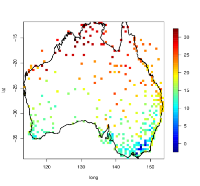
In this section, we apply the proposed $t$ process to a data set of maximum temperature data observed in Australia. Specifically, we consider a subset of a global data set of merged maximum daily temperature measurements from the Global Surface Summary of Day data (GSOD) with European Climate Assessment &Dataset (ECA&D) data in July 2011. The dataset is described in detail in Kilibarda et al. (2014) and it is available in the R package meteo. The subset we consider is depicted in Figure 7 (a) and consists of the maximum temperature observed on July 5 in $446$ location sites, $y(\bm{s}_{i})$, $i=1,\ldots,446$, in the region with longitude $[110,154]$ and latitude $[-39,-12]$.

(a)	(b)

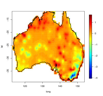
Figure 7: From left to right: a) spatial locations of maximum temperature in Australia in July 2011 and b) prediction of residuals of the estimated $t$ process.

Spatial coordinates are given in longitude and latitude expressed as decimal degrees and we consider the proposed $t$ process defined on the planet Earth sphere approximation $\mathbb{S}^{2}=\{\bm{s}\in\mathbb{R}^{3}:||\bm{s}||=6371\}$. The first process we use to model this dataset is a $t$ process:

$$Y_{\nu}(\bm{s})=\beta_{0}+\beta_{1}X(\bm{s})+\sigma Y^{*}_{\nu}(\bm{s}),\;\;\;\bm{s}\in\mathbb{S}^{2}$$ (5.1)

where $Y^{*}_{\nu}$ is a standard $t$ process. Here, $X(\bm{s})$ is a covariate called geometric temperature which represents the geometric position of a particular location on Earth and the day of the year (Kilibarda et al., 2014). As a comparison, we also consider a Gaussian process:

$$Y(\bm{s})=\beta_{0}+\beta_{1}X(\bm{s})+\sigma G(\bm{s}),\quad\bm{s}\in\mathbb{S}^{2}$$ (5.2)

where $G$ is a standard Gaussian process. We assume that the underlying geodesically isotropic correlation function (Gneiting, 2013; Porcu et al., 2016) is of the Matérn and generalized Wendland type. A preliminary estimation of the $t$ and Gaussian processes, including the smoothness parameters, highlights a multimodality of the (pairwise) likelihood surface, for both correlation models and a not mean-square differentiability of the process. For this reason, we fix the smoothness parameters and we consider the underlying correlation models ${\cal M}_{\alpha,0.5}(d_{GC})=e^{-d_{GC}/\alpha}$ and ${\cal GW}_{\alpha,0,5}(d_{GC})=(1-d_{GC}/\alpha)_{+}^{5}$ where, given two spherical points $\bm{s}_{i}=(\mbox{lon}_{i},\mbox{lat}_{i})$ and $\bm{s}_{j}=(\mbox{lon}_{j},\mbox{lat}_{j})$, $d_{GC}(\bm{s}_{i},\bm{s}_{j})=6371\theta_{ij},$ is the great circle distance. Here $\theta_{ij}=\arccos\{\sin a_{i}\sin a_{j}+\cos a_{i}\cos a_{j}\cos(b_{i}-b_{j})\}$ is the great circle distance on the unit sphere with $a_{i}=(\mbox{lat}_{i})\pi/180$, $a_{j}=(\mbox{lat}_{j})\pi/180$, $b_{i}=(\mbox{lon}_{i})\pi/180$, $b_{j}=(\mbox{lon}_{j})\pi/180$.

For the $t$ process the parameters were estimated using $wpl$ using the bivariate $t$ distribution with the two-step method described in Section 4 and using the weight function (4.2) with $d_{ij}=150$ Km. It turns out that the estimation at the first step leads to fix $\nu=4$ in the second step, irrespective of the correlation model. We also consider a Gaussian misspecified standard likelihood and $wpl$ estimation as described in Section 4.3 i.e. we estimate using the Gaussian process (5.2) with the $t$ correlation model 2.6 fixing $\nu=4$.

In addition, we compute the standard error estimation, PLIC and BLIC values through parametric bootstrap estimation of the inverse of the Godambe information matrix (Bai et al., 2014). For standard maximum likelihood we compute the standard errors as the square root of diagonal elements of the inverse of Fisher Information matrix (Mardia and Marshall, 1984). The results are summarized in Table 5. Note that the regression parameters estimates are quite similar for the $t$ and Gaussian processes, irrespective of the correlation model. Furthermore, we note that the standard Gaussian process assigns lower spatial dependence and stronger variance compared to the other cases. Finally, for each correlation model, both the (pairwise) likelihood information criterion PLIC and BLIC select for the pairwise case the $t$ model and for the standard case the Gaussian model with $t$ correlation function.

Matérn
	Method	$\hat{\beta}_{0}$	$\hat{\beta}_{1}$	$\hat{\alpha}$	$\hat{\sigma}^{2}$	PLIC	BLIC	RMSE	MAE	CRPS
$t$	Pairwise	$6.652$	$0.994$	$58.582$	$7.589$	$23906$	$24689$	$2.775$	$2.138$	$1.807$
		$(1.192)$	$(0.107)$	$(13.492)$	$(1.451)$
Missp-Gaussian	Pairwise	$5.656$	$1.064$	$72.435$	$7.062$	$24680$	$26172$	$2.743$	$2.112$	$1.809$
		$(1.514)$	$(0.130)$	$(18.303)$	$(2.024)$
Missp-Gaussian	Standard	$5.673$	$1.050$	$63.437$	$5.385$	$2228$	$2244$	$2.755$	$2.119$	$1.813$
		$(0.660)$	$(0.045)$	$(10.41)$	$(0.432)$
Gaussian	Standard	$5.508$	$1.060$	$40.484$	$10.762$	$2240$	$2257$	$2.812$	$2.155$	$1.815$
		$(0.558)$	$(0.039)$	$(5.346)$	$(0.813)$
Wendland
	Method	$\hat{\beta}_{0}$	$\hat{\beta}_{1}$	$\hat{\alpha}$	$\hat{\sigma}^{2}$	PLIC	BLIC	RMSE	MAE	CRPS
$t$	Pairwise	$6.6375$	$0.995$	$331.70$	$7.622$	$23890$	$24624$	$2.796$	$2.155$	$1.807$
		$(1.134)$	$(0.103)$	$(69.03)$	$(1.482)$
Missp-Gaussian	Pairwise	$5.647$	$1.065$	$404.81$	$7.080$	$24657$	$26100$	$2.760$	$2.127$	$1.810$
		$(1.446)$	$(0.124)$	$(92.99)$	$(2.032)$
Missp-Gaussian	Standard	$5.579$	$1.056$	$349.90$	$5.485$	$2232$	$2249$	$2.774$	$2.134$	$1.815$
		$(0.618)$	$(0.042)$	$(52.030)$	$(0.434)$
Gaussian	Standard	$5.400$	$1.066$	$225.89$	$11.081$	$2250$	$2266$	$2.846$	$2.177$	$1.820$
		$(0.530)$	$(0.038)$	$(27.72)$	$(0.835)$

Table 5: Estimates for the $t$ process using $wpl$ with bivariate $t$ distribution and misspecified (full and weighted pairwise) Gaussian likelihood and for the Gaussian process using standard likelihood with associated standard error (in parenthesis) and PLIC and BLIC values, when estimating the Australian maximum temperature dataset using two correlation models: ${\cal M}_{\alpha,0.5}$ and ${\cal GW}_{\alpha,0,5}$. Last three columns: associated empirical mean of RMSEs, MAEs and CRPSs.

Given the estimation of the mean regression and variance parameters of the $t$ process, the estimated residuals

$$\hat{{Y}}^{*}_{4}(\bm{s}_{i})=\frac{y(\bm{s}_{i})-(\hat{\beta}_{0}+\hat{\beta}_{1}X(\bm{s}_{i}))}{(\hat{\sigma}^{2})^{\frac{1}{2}}}\quad i=1,\ldots N$$

can be viewed as a realization of the process $Y^{*}_{4}$. Similarly we can compute the Gaussian residuals. For the $t$ process we use the $wpl$ estimates obtained with the bivariate $t$ distribution. Both residuals can be useful in order to check the model assumptions, in particular the marginal and dependence assumptions. In the top part of Figure 8 a $qq$-plot of the residuals of the Gaussian and $t$ processes (from left to right) is depicted for the Matérn case. It can be appreciated that the $t$ model overall fits better with respect the Gaussian model even if it seems to fail to model properly the right tail behavior. Moreover, the graphical comparison between the empirical and fitted semivariogram of the residuals (bottom part of Figure 8) highlights an apparent better fitting of the $t$ model.

(a)	(b)
(c)	(d)

Figure 8: Upper part: Q-Q plot of the residuals versus the estimated quantiles in the Gaussian and $t$ models ((a) and (b) respectively). Bottom part: Empirical semi-variogram (dotted points) of the residuals versus the estimated semivariogram (solid line) in the Gaussian and $t$ models ((c) and (d) respectively). Distances are expressed in Km.

We want to further evaluate the predictive performances of Gaussian and $t$ processes using RMSE and MAE as in Section 4.4. Specifically, we use the following resampling approach: we randomly choose 80% of the data to predict and we use the estimates previously obtained in order to compute RMSE and MAE values at the remaining 20% of the spatial locations. We repeat the approach for 2000 times and record all RMSEs and MAEs. Specifically, for each $j-th$ left-out sample $(y_{j}^{L}(\bm{s}_{1}),\ldots,\ldots,y_{j}^{L}(\bm{s}_{K}))$, we compute

$$\overline{\mathrm{RMSE}}_{j}=\left[\frac{1}{K}\sum_{i=1}^{K}\left(y_{j}^{L}(\bm{s}_{i})-\widehat{Y}_{j}^{L}(\bm{s}_{i})\right)^{2}\right]^{\frac{1}{2}}$$

and

$$\overline{\mathrm{MAE}}_{j}=\frac{1}{K}\sum_{i=1}^{K}|y_{j}^{L}(\bm{s}_{i})-\widehat{Y}_{j}^{L}(\bm{s}_{i})|,$$

where $\widehat{Y}_{j}^{L}(\bm{s}_{i})$ is the optimal or the best linear optimal prediction for the Gaussian and $t$ processes respectively. Finally, we compute the overall mean for both Gaussian and $t$ processes and for both correlation models, that is $\mathrm{RMSE}=\sum_{j=1}^{2000}\overline{\mathrm{RMSE}}_{j}/2000$ and $\mathrm{MAE}=\sum_{j=1}^{2000}\overline{\mathrm{MAE}}_{j}/2000$.

Additionally, to evaluate the marginal predictive distribution performance, we also consider, for each sample, the continuous ranked probability score (CRPS) (Gneiting and Raftery, 2007). For a single predictive cumulative distribution function $F$ and a verifying observation $y$, it is defined as:

$$\mathrm{CRPS}(F,y)=\int\limits_{-\infty}^{\infty}(F(t)-\bm{1}_{[y,\infty]}(t))^{2}dt.$$

Specifically, for each $j-th$ left-out sample, we consider the averaged $\mathrm{CRPS}$ for the Gaussian and $t$ distributions as:

$$\overline{\mathrm{CRPS}}_{j}=\frac{1}{K}\sum_{i=1}^{K}\mathrm{CRPS}(F,y_{j}^{L}(\bm{s}_{i}))\quad F=F_{G},F_{Y_{4}},$$ (5.3)

for $j=1,\ldots,2000$. In particular in the Gaussian case

$$CRPS(F_{G},y_{j}^{L}(\bm{s}_{i}))=\sigma\left(\frac{y_{j}^{L}(\bm{s}_{i})-\mu(\bm{s})}{\sigma}\right)\left[2F_{G^{*}(\bm{s})}\left(\frac{y_{j}^{L}(\bm{s}_{i})-\mu(\bm{s})}{\sigma}\right)-1\right]+2\sigma f_{G^{*}(\bm{s})}\left(\frac{y_{j}^{L}(\bm{s}_{i})-\mu(\bm{s})}{\sigma}\right)-\frac{\sigma}{\sqrt{\pi}},$$ (5.4)

and in the $t$ case with $4$ degrees of freedom:

$$CRPS(F_{Y_{4}},y_{j}^{L}(\bm{s}_{i})) =\sigma\left(\frac{y_{j}^{L}(\bm{s}_{i})-\mu(\bm{s})}{\sigma}\right)\left[2F_{Y^{*}_{4}(\bm{s})}\left(\frac{y_{j}^{L}(\bm{s}_{i})-\mu(\bm{s})}{\sigma}\right)-1\right]$$ (5.5)

$$+2\left[\frac{4\sigma^{2}+(y_{j}^{L}(\bm{s}_{i})-\mu(\bm{s}))^{2}}{3\sigma}\right]f_{Y^{*}_{4}(\bm{s})}\left(\frac{y_{j}^{L}(\bm{s}_{i})-\mu(\bm{s})}{\sigma}\right)-\frac{4\sigma B\left(\frac{1}{2},\frac{7}{2}\right)}{3B^{2}\left(\frac{1}{2},2\right)},$$

where $\mu(\bm{s})=\beta_{0}+\beta_{1}X(\bm{s})$. We compute the CRPS in (5.4) and (5.5) plugging-in the estimates of the pairwise and standard (misspecified) likelihood estimation methods of $\beta_{0}$, $\beta_{1}$ and $\sigma$ using the R package scoringRules (Jordan et al., 2019). Finally, we compute the overall mean for both Gaussian and $t$ processes and for both correlation models, that is $\mathrm{CRPS}=\sum_{j=1}^{2000}\overline{\mathrm{CRPS}}_{j}/2000$.

Table 5 reports the estimated RMSE, MAE and CRPS. As a general remark, the $t$ process outperforms the Gaussian process for the three measures of prediction performance irrespective of the method of estimation and for both correlation models. We point out that RMSE and MAE are computed using the optimal predictor in the Gaussian case and the linear optimal in the $t$ case. However, the RMSE and MAE results highlight a better performance for the $t$ process. In addition, a better RMSE and MAE for the Matérn correlation model with respect to the Wendland is apparent, irrespective of the type of process. The proposed $t$ process also leads to a clear better performance of the CRPS with respect to the Gaussian case. In this specific example, the use of the misspecified Gaussian $wpl$ estimates leads to the best results in terms of RMSE and MAE. On the other hand, the best CRPS results are achieved by using the $wpl$ estimates using the proposed $t$ bivariate distribution

Finally, one important goal in spatial modeling of temperature data is to create a high resolution map in a spatial region using the observed data. In Figure 7 (b), we plot a high resolution map of the predicted residuals using the $t$ process with underlying Matérn correlation model estimated with $wpl$.

6 Concluding remarks

We have introduced a new stochastic process with $t$ marginal distributions for regression and dependence analysis when addressing spatial with heavy tails. Our proposal allows overcoming any problem of identifiability associated with previously proposed spatial models with $t$ marginals and, as a consequence, the model parameters can be estimated with just one realization of the process. Additionally, the proposed $t$ process partially inherits some geometrical properties of the ‘parent’ Gaussian process, an appealing feature from a data analysis point of view. We have also proposed a possible generalization, obtaining a new process with the marginal distribution of the skew-$t$ type using the skew-Gaussian process proposed in Zhang and El-Shaarawi (2010).

In our proposal, a possible limitation is the lack of amenable expressions of the associated multivariate distributions. This prevents an inference approach based on the full likelihood and the computation of the optimal predictor. In the first case, our simulation study shows that an inferential approach based on $wpl$, using the bivariate $t$ distribution given in Theorem 2.3, could be an effective solution for estimating the unknown parameters. An alternative less efficient solution that requires smaller computational burden can be obtained by considering a misspecified Gaussian $wpl$ using the correlation function of the $t$ process. In the prediction case, our numerical experiments show that the optimal linear predictor of the $t$ process performs better than the optimal Gaussian predictor when working with spatial data with heavy tails.

Another possible drawback concerns the restriction of the degrees of freedom of the $t$ process to $\nu=3,4,\ldots$. under non-infinite divisibility of the associated Gamma process. This problem could be solved by considering a Gamma process obtained by mixing the proposed Gamma process with a process with beta marginals and using the results in Yeo and Milne (1991); however the mathematics involved with this approach are much more challenging.

The estimation of the skew-$t$ process has not been addressed in this paper since the bivariate distribution in this case is quite complicated. In principle, after a suitable parametrization, Gaussian misspecified $wpl$ can be performed using (3.7) to estimate the parameters of the skew-$t$ process. In this case an additional issue is the behavior of the information matrix when $\eta=0$ (Arellano-Valle and Azzalini, 2013). Finally, a $t$ process with asymmetric marginal distribution can also be obtained by considering some specific transformations of the proposed standard $t$ process as in J. F. Rosco and Pewsey (2011) or under the two-piece distribution framework (Arellano-Valle et al., 2005) and this will be studied in future work.

Appendix A Appendix

A.1 Proof of Theorem 2.1

Proof.

Set $R_{\nu}\equiv W^{-\frac{1}{2}}_{\nu}$. Then the correlation function of $Y^{*}_{\nu}$ is given by

$$\rho_{Y^{*}_{\nu}}(\bm{h})=\left(\frac{\nu-2}{\nu}\right)\left(\operatorname{E}(R_{\nu}(\bm{s}_{i})R_{\nu}(\bm{s}_{j}))\rho(\bm{h})\right).$$ (A.1)

To find a closed form for $\operatorname{E}(R_{\nu}(\bm{s}_{i})R_{\nu}(\bm{s}_{j})$, we need the bivariate distribution of $\bm{R}_{\nu;ij}$ that can be easily obtained from density of the bivariate random vector $\bm{W}_{\nu;ij}$ given by (Bevilacqua et al., 2018):

$$f_{\bm{W}_{\nu;ij}}(w_{i},w_{j})=\frac{2^{-\nu}\nu^{\nu}(w_{i}w_{j})^{\nu/2-1}e^{-\frac{\nu(w_{i}+w_{j})}{2(1-\rho^{2}(\bm{h}))}}}{\Gamma\left(\frac{\nu}{2}\right)(1-\rho^{2}(\bm{h}))^{\nu/2}}\left(\frac{\nu\sqrt{\rho^{2}(\bm{h})w_{i}w_{j}}}{2(1-\rho^{2}(\bm{h}))}\right)^{1-\nu/2}I_{\nu/2-1}\left(\frac{\nu\sqrt{\rho^{2}(\bm{h})w_{i}w_{j}}}{(1-\rho^{2}(\bm{h}))}\right)$$ (A.2)

where $I_{\alpha}(\cdot)$ denotes the modified Bessel function of the first kind of order $\alpha$. Vere-Jones (1967) show the infinite divisibility of $\bm{W}_{\nu;ij}$.

Then, for each $\nu>2$, the bivariate distribution of $\bm{R}_{\nu;ij}$ is given by:

$$f_{\bm{R}_{\nu;ij}}(\bm{r}_{ij})=\frac{2^{-\nu+2}\nu^{\nu}(r_{i}r_{j})^{-\nu-1}e^{-\frac{\nu}{2(1-\rho^{2}(\bm{h}))}\left(\frac{1}{r^{2}_{i}}+\frac{1}{r^{2}_{j}}\right)}}{\Gamma\left(\frac{\nu}{2}\right)(1-\rho^{2}(\bm{h}))^{\nu/2}}\left(\frac{\nu\rho(\bm{h})}{2(1-\rho^{2}(\bm{h}))r_{i}r_{j}}\right)^{1-\frac{\nu}{2}}I_{\frac{\nu}{2}-1}\left(\frac{\nu\rho(\bm{h})}{(1-\rho^{2}(\bm{h}))r_{i}r_{j}}\right)$$ (A.3)

Using the identity ${}_{0}F_{1}(;b;x)=\Gamma(b)x^{(1-b)/2}I_{b-1}(2\sqrt{x})$ and the series expansion of hypergeometric function ${}_{0}F_{1}$ in (A.3) we have

$$\operatorname{E}(R^{a}(\bm{s}_{i})R^{b}(\bm{s}_{j})) =\frac{2^{-\nu+2}\nu^{\nu}}{\Gamma^{2}\left(\frac{\nu}{2}\right)(1-\rho^{2}(\bm{h}))^{\nu/2}}\int\limits_{\mathbb{R}_{+}^{2}}r_{i}^{-\nu+a-1}r_{j}^{-\nu+b-1}e^{-\frac{\nu}{2(1-\rho^{2}(\bm{h}))r_{i}^{2}}}e^{-\frac{\nu}{2(1-\rho^{2}(\bm{h}))r_{j}^{2}}}$$

$$\times{}_{0}F_{1}\left(\frac{\nu}{2};\frac{\nu^{2}\rho^{2}(\bm{h})}{4(1-\rho^{2}(\bm{h}))^{2}r^{2}_{i}r^{2}_{j}}\right)d\bm{r}_{ij}$$

$$=\frac{2^{-\nu+2}\nu^{\nu}}{\Gamma^{2}\left(\frac{\nu}{2}\right)(1-\rho^{2}(\bm{h}))^{\nu/2}}\sum\limits_{k=0}^{\infty}\int\limits_{\mathbb{R}_{+}^{2}}r_{i}^{-\nu+a-2k-1}r_{j}^{-\nu+b-2k-1}e^{-\frac{\nu}{2(1-\rho^{2}(\bm{h}))r_{i}^{2}}}e^{-\frac{\nu}{2(1-\rho^{2}(\bm{h}))r_{j}^{2}}}$$

$$\times\frac{1}{k!\left(\frac{\nu}{2}\right)_{k}}\left(\frac{\rho^{2}(\bm{h})\nu^{2}}{4(1-\rho^{2}(\bm{h}))}\right)^{k}d\bm{r}_{ij}$$

$$=\frac{2^{-\nu+2}\nu^{\nu}}{\Gamma^{2}\left(\frac{\nu}{2}\right)(1-\rho^{2}(\bm{h}))^{\nu/2}}\sum\limits_{k=0}^{\infty}\frac{I(k)}{k!\left(\frac{\nu}{2}\right)_{k}}\left(\frac{\rho^{2}(\bm{h})\nu^{2}}{4(1-\rho^{2}(\bm{h}))}\right)^{k}$$ (A.4)

where, using Fubini’s Theorem

$$I(k)=\int\limits_{\mathbb{R}_{+}}r_{i}^{-\nu+a-2k-1}e^{-\frac{\nu}{2(1-\rho^{2}(\bm{h}))r_{i}^{2}}}dr_{i}\int\limits_{\mathbb{R}_{+}}r_{j}^{\nu+b-2k-1}e^{-\frac{\nu}{2(1-\rho^{2}(\bm{h}))r_{j}^{2}}}dr_{j}$$

Using the univariate density $f_{R_{\nu}(\bm{s})}(r)=2\left(\frac{\nu}{2}\right)^{\nu/2}r^{-\nu-1}e^{-\frac{\nu}{2r^{2}}}/\Gamma\left(\frac{\nu}{2}\right)$, we obtain

$$I(k) =\Gamma\left(\frac{\nu-a}{2}+k\right)\Gamma\left(\frac{\nu-b}{2}+k\right)2^{\frac{\nu-a}{2}+k-1}2^{\frac{\nu-b}{2}+k-1}\left(\frac{(1-\rho^{2}(\bm{h}))}{\nu}\right)^{\frac{\nu-a}{2}+k}\left(\frac{(1-\rho^{2}(\bm{h}))}{\nu}\right)^{\frac{\nu-b}{2}+k}$$ (A.5)

and combining equations (A.5) and (A.1), we obtain

$$\operatorname{E}(R^{a}(\bm{s}_{i})R^{b}(\bm{s}_{j})) =\frac{2^{-(a+b)/2}\nu^{(a+b)/2}(1-\rho^{2}(\bm{h}))^{(\nu-a-b)/2}\Gamma\left(\frac{\nu-a}{2}\right)\Gamma\left(\frac{\nu-b}{2}\right)}{\Gamma^{2}\left(\frac{\nu}{2}\right)}\sum\limits^{\infty}_{k=0}\frac{\left(\frac{\nu-a}{2}\right)_{k}\left(\frac{\nu-b}{2}\right)_{k}}{k!\left(\frac{\nu}{2}\right)_{k}}\rho^{2k}(\bm{h})$$

$$=\frac{2^{-(a+b)/2}\nu^{(a+b)/2}(1-\rho^{2}(\bm{h}))^{(\nu-a-b)/2}\Gamma\left(\frac{\nu-a}{2}\right)\Gamma\left(\frac{\nu-b}{2}\right)}{\Gamma^{2}\left(\frac{\nu}{2}\right)}{}_{2}F_{1}\left(\frac{\nu-a}{2},\frac{\nu-b}{2};\frac{\nu}{2};\rho^{2}(\bm{h})\right)$$

Then, using the Euler transformation, we obtain

$$\operatorname{E}(R_{\nu}^{a}(\bm{s}_{i})R_{\nu}^{b}(\bm{s}_{j})) =\frac{2^{-(a+b)/2}\nu^{(a+b)/2}}{\Gamma^{2}\left(\frac{\nu}{2}\right)}\Gamma\left(\frac{\nu-a}{2}\right)\Gamma\left(\frac{\nu-b}{2}\right){}_{2}F_{1}\left(\frac{a}{2},\frac{b}{2};\frac{\nu}{2};\rho^{2}(\bm{h})\right)$$ (A.6)

for $\nu>a$ and $\nu>b$. Finally, setting $a=b=1$ in (A.6) and using it in (A.1) we obtain (2.6). ∎

A.2 Proof of Theorem 2.2

Proof.

If $G$ is a weakly stationary Gaussian process with correlation $\rho(\bm{h})$ then from (2.6) it is straightforward to see that $Y^{*}_{\nu}$ is also weakly stationary. Points b) and c) can be shown using the relations between the geometrical properties of a stationary process and the associated correlation. Specifically, the mean-square continuity and the $m$-times mean-square differentiability of $Y^{*}_{\nu}$ are equivalent to the continuity and $2m$-times differentiability of $\rho_{Y^{*}_{\nu}}(\bm{h})$ at $\bm{h}=\bm{0}$, respectively (Stein, 1999). Recall that the correlation function of $Y^{*}_{\nu}$ is given by:

$$\rho_{Y^{*}_{\nu}}(\bm{h})=a(\nu)\left[{}_{2}F_{1}\left(\frac{1}{2},\frac{1}{2};\frac{\nu}{2};\rho^{2}(\bm{h})\right)\rho(\bm{h})\right].$$ (A.7)

with $a(\nu)=\frac{(\nu-2)\Gamma^{2}\left(\frac{\nu-1}{2}\right)}{2\Gamma^{2}\left(\frac{\nu}{2}\right)}$. Using (2.5) it can be easily seen that $\rho(\bm{\bm{0}})=1$ if and only if $\rho_{Y^{*}_{\nu}}(\bm{0})=1$. Then $Y^{*}_{\nu}$ is mean-square continuous if and only if $G$ is mean-square continuous.

For the mean square differentiability, let $G$ $m-$times mean square differentiable. Using iteratively the $n-$th derivative of the ${}_{2}F_{1}$ function with respect to $x$:

$${}_{2}F^{(n)}_{1}(a,b,c,x)=\frac{(a)_{n}(b)_{n}}{(c)_{n}}{}_{2}F_{1}(a+n,b+n,c+n,x),\qquad n=1,2,\ldots$$ (A.8)

and applying the convergence condition $c>b+a$ of identity (2.5), it can be shown that $\rho^{(2m)}_{Y^{*}_{\nu}}(\bm{h})|_{\bm{h}=\bm{0}}<\infty$ if $\nu>2(2m+1)$ and, as a consequence, $Y^{*}_{\nu}$ is $m-$times mean square differentiable under this condition. On the other hand if $\nu\leq 2(2m+1)$ then $Y^{*}_{\nu}$ is $(m-k)$-times mean-square differentiable if $2(2(m-k)+1)<\nu\leq 2(2(m-k)+3)$, for $k=1,\ldots,m$.

For instance, let assume that $G$ is $1-$times mean square differentiable. This implies that $\rho^{(i)}(\bm{h})|_{\bm{h}=\bm{0}}<\infty$, $i=1,2$. Applying (A.8) to (A.7), the second derivative of $\rho_{Y^{*}_{\nu}}(\bm{h})$ is given by:

$$\rho^{(2)}_{Y^{*}_{\nu}}(\bm{h}) =\frac{a(\nu)}{\nu(\nu+2)}\bigg{[}(6+3\nu){}_{2}F_{1}\left(1.5,1.5;1+\frac{\nu}{2};\rho^{2}(\bm{h})\right)\rho(\bm{h})\{\rho^{(1)}(\bm{h})\}^{2}$$

$$+9{}_{2}F_{1}\left(2.5,2.5;2+\frac{\nu}{2};\rho^{2}(\bm{h})\right)\rho^{3}(\bm{h})\{\rho^{(1)}(\bm{h})\}^{2}+\nu(2+\nu){}_{2}F_{1}\left(0.5,0.5;\frac{\nu}{2};\rho^{2}(\bm{h})\right)\rho^{(2)}(\bm{h})$$

$$+(2+\nu){}_{2}F_{1}\left(1.5,1.5;1+\frac{\nu}{2};\rho^{2}(\bm{h})\right)\rho^{2}(\bm{h})\rho^{(2)}(\bm{h})\bigg{]}$$

Then, applying the convergence condition of identity (2.5), $\rho^{(2)}_{Y^{*}_{\nu}}(\bm{h})|_{\bm{h}=\bm{0}}<\infty$ if $2+\nu/2>5$ that is $\nu>6$. Therefore $Y^{*}_{\nu}$ is $1-$times mean square differentiable if $\nu>6$ and $0-$times mean square differentiable if $2<\nu\leq 6$.

Point d) can be shown recalling that a process $F$ is long-range dependent if the correlation of $F$ is such that $\int_{\mathbb{R}^{n}_{+}}|\rho_{F}(\bm{h})|d^{n}\bm{h}=\infty$ (Lim and Teo, 2009). Direct inspection, using series expansion of the hypergeometric function, shows that $\int_{\mathbb{R}^{n}_{+}}|\rho_{Y^{*}_{\nu}}(\bm{h})|d^{n}\bm{h}=\infty$ if and only if $\int_{\mathbb{R}^{n}_{+}}|\rho(\bm{h})|d^{n}\bm{h}=\infty$ and, as a consequence, $Y^{*}_{\nu}$ has long-range dependence if and only if $G$ has long-range dependence.

Finally, note that if $\nu>2$ then $a(\nu){}_{2}F_{1}\left(\frac{1}{2},\frac{1}{2};\frac{\nu}{2};0\right)=a(\nu)$, $a(\nu){}_{2}F_{1}\left(\frac{1}{2},\frac{1}{2};\frac{\nu}{2};1\right)=1$ and $a(\nu){}_{2}F_{1}\left(\frac{1}{2},\frac{1}{2};\frac{\nu}{2};x^{2}\right)$ is not decreasing in $0\leq x\leq 1$. This implies $a(\nu){}_{2}F_{1}\left(\frac{1}{2},\frac{1}{2};\frac{\nu}{2};x^{2}\right)\leq 1$ that is $\rho_{Y^{*}_{\nu}}(\bm{h})\leq\rho(\bm{h})$. Moreover, $\lim\limits_{\nu\to\infty}a(\nu)=1$ and using series expansion of the hypergeometric function:

$$\lim\limits_{\nu\rightarrow\infty}{}_{2}F_{1}\left(\frac{1}{2},\frac{1}{2};\frac{\nu}{2};\rho(\bm{h})^{2}\right) =\lim\limits_{\nu\rightarrow\infty}\bigg{[}1+\frac{\left(\frac{1}{2}\right)^{2}_{1}\rho(\bm{h})^{2}}{1\left(\frac{\nu}{2}\right)_{1}}+\frac{\left(\frac{1}{2}\right)^{2}_{2}\rho(\bm{h})^{4}}{1\left(\frac{\nu}{2}\right)_{2}}+\ldots+\frac{\left(\frac{1}{2}\right)^{2}_{k}\rho(\bm{h})^{2k}}{1\left(\frac{\nu}{2}\right)_{k}}+\ldots\bigg{]}$$

$$=\lim\limits_{\nu\rightarrow\infty}\bigg{[}1+\frac{2\rho(\bm{h})^{2}}{\nu}+\frac{\left(\frac{1}{2}\right)^{2}\left(\frac{1}{2}+1\right)^{2}\rho(\bm{h})^{2}}{2!\left(\frac{\nu}{2}\right)\left(\frac{\nu}{2}+1\right)}$$

$$+\ldots+\frac{\left(\frac{1}{2}\right)^{2}\left(\frac{1}{2}+1\right)^{2}\cdots\left(\frac{1}{2}+k-1\right)^{2}\rho(\bm{h})^{2k}}{k!\left(\frac{\nu}{2}\right)\left(\frac{\nu}{2}+1\right)\cdots\left(\frac{\nu}{2}+k-1\right)}+\ldots\bigg{]}$$

$$=1.$$

This implies $\lim\limits_{\nu\to\infty}\rho_{Y^{*}_{\nu}}(\bm{h})=\rho(\bm{h})$. ∎

A.3 Proof of Theorem 2.3

Proof.

Using the identity ${}_{0}F_{1}(;b;x)=\Gamma(b)x^{(1-b)/2}I_{b-1}(2\sqrt{x})$ and the series expansion of hypergeometric function ${}_{0}F_{1}$, then under the transformation $g_{i}=y_{i}\sqrt{w_{i}}$ and $g_{j}=y_{j}\sqrt{w_{j}}$ with Jacobian $J((g_{i},g_{j})\to(y_{i},y_{j}))=(w_{i}w_{j})^{1/2}$, we have:

$$f_{\bm{Y}^{*}_{ij}}(\bm{y}_{ij}) =\int\limits_{\mathbb{R}_{+}^{2}}f_{\bm{G}_{ij}|\bm{W}_{ij}}(\bm{g}_{ij}|\bm{w}_{ij})f_{\bm{W}_{ij}}(\bm{w}_{ij})Jd\bm{w}_{ij}$$

$$=\frac{2^{-\nu}\nu^{\nu}}{2\pi\Gamma^{2}\left(\frac{\nu}{2}\right)(1-\rho^{2}(\bm{h}))^{(\nu+1)/2}}\int\limits_{\mathbb{R}^{2}_{+}}(w_{i}w_{j})^{(\nu+1)/2-1}e^{-\frac{1}{2(1-\rho^{2}(\bm{h}))}\left[w_{i}y_{i}^{2}+w_{j}y_{j}^{2}-2\rho(\bm{h})\sqrt{w_{i}w_{j}}y_{i}y_{j}\right]}$$

$$\times e^{-\frac{\nu(w_{i}+w_{j})}{2(1-\rho^{2}(\bm{h}))}}{}_{0}F_{1}\left(\frac{\nu}{2};\frac{\nu^{2}\rho^{2}(\bm{h})w_{i}w_{j}}{4(1-\rho^{2}(\bm{h}))^{2}}\right)d\bm{w}_{ij}$$

$$=\frac{2^{-\nu}\nu^{\nu}}{2\pi\Gamma^{2}\left(\frac{\nu}{2}\right)(1-\rho^{2}(\bm{h}))^{(\nu+1)/2}}\int\limits_{\mathbb{R}^{2}_{+}}(w_{i}w_{j})^{(\nu+1)/2-1}e^{-\frac{1}{2(1-\rho^{2}(\bm{h}))}\left[y_{i}^{2}-2\rho(\bm{h})\sqrt{\frac{w_{j}}{w_{i}}}y_{i}y_{j}+\nu\right]w_{i}}e^{-\frac{(y_{j}^{2}+\nu)w_{j}}{2(1-\rho^{2}(\bm{h}))}}$$

$$\times\sum\limits_{k=0}^{\infty}\frac{1}{k!\left(\frac{\nu}{2}\right)_{k}}\left(\frac{\nu^{2}\rho^{2}(\bm{h})w_{i}w_{j}}{4(1-\rho^{2}(\bm{h}))^{2}}\right)^{k}d\bm{w}_{ij}$$

$$=\frac{2^{-\nu}\nu^{\nu}}{2\pi\Gamma^{2}\left(\frac{\nu}{2}\right)(1-\rho^{2}(\bm{h}))^{(\nu+1)/2}}\sum\limits_{k=0}^{\infty}\frac{I(k)}{k!\left(\frac{\nu}{2}\right)_{k}}\left(\frac{\nu^{2}\rho^{2}(\bm{h})}{4(1-\rho^{2}(\bm{h}))^{2}}\right)^{k}$$ (A.9)

using (3.462.1) of Gradshteyn and Ryzhik (2007), we obtain

$$I(k) =\int\limits_{\mathbb{R}_{+}}w_{j}^{(\nu+1)/2+k-1}e^{-\frac{(y_{j}^{2}+\nu)w_{j}}{2(1-\rho^{2}(\bm{h}))}}\left[\int\limits_{\mathbb{R}_{+}}w_{i}^{(\nu+1)/2+k-1}e^{\left[-\frac{(y_{i}^{2}+\nu)}{2(1-\rho^{2}(\bm{h}))}w_{i}-\frac{\rho(\bm{h})\sqrt{w_{j}}y_{i}y_{j}}{(\rho^{2}(\bm{h})-1)}\sqrt{w_{i}}\right]}dw_{i}\right]dw_{j}$$

$$=2\left(\frac{y_{i}^{2}+\nu}{(1-\rho^{2}(\bm{h}))}\right)^{-\left(\frac{\nu+1}{2}+k\right)}\Gamma\left(\nu+1+2k\right)\int\limits_{\mathbb{R}_{+}}w_{j}^{(\nu+1)/2+k-1}e^{\left[\frac{\rho^{2}(\bm{h})y_{i}^{2}y_{j}^{2}}{4(1-\rho^{2}(\bm{h}))(y_{i}^{2}+\nu)}-\frac{(y_{j}^{2}+\nu)}{2(1-\rho^{2}(\bm{h}))}\right]w_{j}}$$

$$\times D_{-(\nu+1+2k)}\left(-\frac{\rho(\bm{h})y_{i}y_{j}\sqrt{w_{j}}}{\sqrt{(1-\rho^{2}(\bm{h}))(y_{i}^{2}+\nu)}}\right)dw_{j}$$

$$=2\left(\frac{y_{i}^{2}+\nu}{(1-\rho^{2}(\bm{h}))}\right)^{-\left(\frac{\nu+1}{2}+k\right)}\Gamma\left(\nu+1+2k\right)A(k)$$ (A.10)

where $D_{n}(x)$ is the parabolic cylinder function. Now, considering (9.240) of Gradshteyn and Ryzhik (2007):

$$D_{-(\nu+1+2k)}\left(-\frac{\rho(\bm{h})y_{i}y_{j}\sqrt{w_{j}}}{\sqrt{(1-\rho^{2}(\bm{h}))(y_{i}^{2}+\nu)}}\right) =b_{1}e^{-\frac{\rho^{2}(\bm{h})y^{2}_{i}y^{2}_{j}w_{j}}{4(1-\rho^{2}(\bm{h}))(y_{i}^{2}+\nu)}}$$

$$\times{}_{1}F_{1}\left(\frac{\nu+1}{2}+k;\frac{1}{2};\frac{\rho^{2}(\bm{h})y^{2}_{i}y^{2}_{j}w_{j}}{2(1-\rho^{2}(\bm{h}))(y_{i}^{2}+\nu)}\right)$$

$$+b_{2}\sqrt{w_{j}}e^{-\frac{\rho^{2}(\bm{h})y^{2}_{i}y^{2}_{j}w_{j}}{4(1-\rho^{2}(\bm{h}))(y_{i}^{2}+\nu)}}$$

$$\times{}_{1}F_{1}\left(\frac{\nu}{2}+k+1;\frac{3}{2};\frac{\rho^{2}(\bm{h})y^{2}_{i}y^{2}_{j}w_{j}}{2(1-\rho^{2}(\bm{h}))(y_{i}^{2}+\nu)}\right)$$ (A.11)

where $b_{1}=\frac{2^{-(\nu+1)/2+k}\sqrt{\pi}}{\Gamma\left(\frac{\nu}{2}+k+1\right)}$ and $b_{2}=\frac{2^{-\nu/2-k}\sqrt{\pi}\rho(\bm{h})y_{i}y_{j}}{\Gamma\left(\frac{\nu+1}{2}+k\right)\sqrt{(1-\rho^{2}(\bm{h}))(y_{i}^{2}+\nu)}}$. Replacing equations (A.3) in (A.3) and using (7.621.4) of Gradshteyn and Ryzhik (2007), we obtain

$$A(k) =b_{1}\int\limits_{\mathbb{R}_{+}}w_{j}^{(\nu+1)/2+k-1}e^{-\frac{(y^{2}_{j}+\nu)}{2(1-\rho^{2}(\bm{h}))}w_{j}}{}_{1}F_{1}\left(\frac{\nu+1}{2}+k;\frac{1}{2};\frac{\rho^{2}(\bm{h})y^{2}_{i}y^{2}_{j}w_{j}}{2(1-\rho^{2}(\bm{h}))(y_{i}^{2}+\nu)}\right)dw_{j}$$

$$+b_{2}\int\limits_{\mathbb{R}_{+}}w_{j}^{\nu/2+k+1-1}e^{-\frac{(y^{2}_{j}+\nu)}{2(1-\rho^{2}(\bm{h}))}w_{j}}{}_{1}F_{1}\left(\frac{\nu}{2}+k+1;\frac{3}{2};\frac{\rho^{2}(\bm{h})y^{2}_{i}y^{2}_{j}w_{j}}{2(1-\rho^{2}(\bm{h}))(y_{i}^{2}+\nu)}\right)dw_{j}$$

$$=b_{1}\Gamma\left(\frac{\nu+1}{2}+k\right)\left(\frac{y^{2}_{j}+\nu}{2(1-\rho^{2}(\bm{h}))}\right)^{-\frac{(\nu+1)}{2}-k}{}_{2}F_{1}\left(\frac{\nu+1}{2}+k,\frac{\nu+1}{2}+k;\frac{1}{2};\frac{\rho^{2}(\bm{h})y^{2}_{i}y^{2}_{j}}{(y_{i}^{2}+\nu)(y_{j}^{2}+\nu)}\right)$$

$$+b_{2}\Gamma\left(\frac{\nu}{2}+k+1\right)\left(\frac{y^{2}_{j}+\nu}{2(1-\rho^{2}(\bm{h}))}\right)^{-\frac{\nu}{2}-k-1}{}_{2}F_{1}\left(\frac{\nu}{2}+k+1,\frac{\nu}{2}+k+1;\frac{3}{2};\frac{\rho^{2}(\bm{h})y^{2}_{i}y^{2}_{j}}{(y_{i}^{2}+\nu)(y_{j}^{2}+\nu)}\right)$$ (A.12)

finally, combining equations (A.3), (A.3) and (A.3), we obtain

$$f_{\bm{Y}^{*}_{ij}}(\bm{y}_{ij}) =\frac{\nu^{\nu}[(y_{i}^{2}+\nu)(y_{j}^{2}+\nu)]^{-(\nu+1)/2}\Gamma^{2}\left(\frac{\nu+1}{2}\right)}{\pi\Gamma^{2}\left(\frac{\nu}{2}\right)(1-\rho^{2}(\bm{h}))^{-(\nu+1)/2}}\sum\limits_{k=0}^{\infty}\frac{\left(\frac{\nu+1}{2}\right)^{2}_{k}}{k!\left(\frac{\nu}{2}\right)_{k}}\left(\frac{\nu^{2}\rho^{2}(\bm{h})}{(y_{i}^{2}+\nu)(y_{j}^{2}+\nu)}\right)^{k}$$

$$\times{}_{2}F_{1}\left(\frac{\nu+1}{2}+k,\frac{\nu+1}{2}+k;\frac{1}{2};\frac{\rho^{2}(\bm{h})y_{i}^{2}y_{j}^{2}}{(y_{i}^{2}+\nu)(y_{j}^{2}+\nu)}\right)$$

$$+\frac{\rho(\bm{h})y_{i}y_{j}\nu^{\nu+2}[(y_{i}^{2}+\nu)(y_{j}^{2}+\nu)]^{-\nu/2-1}}{2\pi(1-\rho^{2}(\bm{h}))^{-(\nu+1)/2}}\sum\limits_{k=0}^{\infty}\frac{\left(\frac{\nu}{2}+1\right)^{2}_{k}}{k!\left(\frac{\nu}{2}\right)_{k}}\left(\frac{\nu^{2}\rho^{2}(\bm{h})}{(y_{i}^{2}+\nu)(y_{j}^{2}+\nu)}\right)^{k}$$

$$\times{}_{2}F_{1}\left(\frac{\nu}{2}+k+1,\frac{\nu}{2}+k+1;\frac{3}{2};\frac{\rho^{2}(\bm{h})y_{i}^{2}y_{j}^{2}}{(y_{i}^{2}+\nu)(y_{j}^{2}+\nu)}\right)$$

and using (4.3) we obtain theorem 2.3. ∎

A.4 Proof of Theorem 3.1

Proof.

Consider $\bm{U}=(U(\bm{s}_{1}),\ldots,U(\bm{s}_{n}))^{T}$, $\bm{V}=(|X_{1}(\bm{s}_{1})|,\ldots,|X_{1}(\bm{s}_{n})|)^{T}$, $\bm{Q}=(X_{2}(\bm{s}_{1}),\ldots,X_{2}(\bm{s}_{n}))^{T}$ where $\bm{X}_{k}=(X_{k}(\bm{s}_{1}),\ldots,X_{k}(\bm{s}_{n}))^{T}\sim N_{n}(\bm{0},\Omega)$, for $k=1,2$, which are assumed to be independent. By definition of the skew-Gaussian process in (3.1) we have:

$$\bm{U}=\bm{\alpha}+\eta\bm{V}+\omega\bm{Q}$$

where, by assumption $\bm{V}$ and $\bm{Q}$ are independent. Thus, by conditioning on $\bm{V}=\bm{v}$, we have $\bm{U}|\bm{V}=\bm{v}\sim N_{n}(\bm{\alpha}+\eta\bm{v},\omega^{2}\Omega)$, from which we obtain

$$f_{\bm{U}}(\bm{u})=\int\limits_{\mathbb{R}^{n}}\phi_{n}(\bm{u};\bm{\alpha}+\eta\bm{v},\omega^{2}\Omega)f_{\bm{V}}(\bm{v})d\bm{v}$$

To solve this integral we need $f_{\bm{V}}(\bm{v})$, $i.e$., the joint density of $\bm{V}=(|X_{1}(\bm{s}_{1})|,\ldots,|X_{1}(\bm{s}_{n})|)^{T}$. Let $\bm{X}_{k}=(X_{1},\ldots,X_{n})^{T}=(X_{1}(\bm{s}_{1}),\ldots,X_{1}(\bm{s}_{n}))^{T}$ and $\bm{V}=(|X_{1}|,\ldots,|X_{n}|)^{T}$. Additionally, consider the diagonal matrices $\bm{D}(\bm{l})=\text{diag}\{l_{1},\ldots,l_{n}\}$, with $\bm{l}=(l_{1},\ldots,l_{n})\in\{-1,+1\}^{n}$, which are such that $\bm{D}(\bm{l})^{2}$ is the identity matrix. Since $\bm{l}\circ\bm{v}=\bm{D}(\bm{l})\bm{v}$ (the componentwise product) and $\bm{X}\sim N_{n}(\bm{0},\Omega)$, we then have

$$F_{\bm{V}}(\bm{v}) =Pr(\bm{V}\leq\bm{v})=Pr(|\bm{X}|\leq\bm{v})=Pr(-\bm{v}\leq\bm{X}\leq\bm{v})$$

$$=\sum\limits_{\bm{l}\in\{-1,+1\}^{n}}(-1)^{N_{-}}\Phi_{n}(\bm{D}(\bm{l})\bm{v};\bm{0},\Omega),\;\;\;\;(N_{-}=\sum\limits_{i=1}^{n}I_{l_{i}=1}\text{det}\{\bm{D}(\bm{l})\})$$

$$=\sum\limits_{\bm{l}\in\{-1,+1\}^{n}}\text{det}\{\bm{D}(\bm{l})\}\Phi_{n}(\bm{D}(\bm{l})\bm{v};\bm{0},\Omega)$$

Hence, by using that

$$\frac{\partial^{n}\Phi_{n}(\bm{D}(\bm{l})\bm{v};\bm{0},\Omega)}{\partial v_{1}\cdots\partial v_{n}}=\text{det}\{\bm{D}(\bm{l})\}\Phi_{n}(\bm{D}(\bm{l})\bm{v};\bm{0},\Omega)$$

we find that the joint density of $\bm{V}$ is

$$f_{\bm{V}}(\bm{v}) =\sum\limits_{\bm{l}\in\{-1,+1\}^{n}}[\text{det}\{\bm{D}(\bm{l})\}]^{2}\phi_{n}(\bm{D}(\bm{l})\bm{v};\bm{0},\Omega)$$

$$=\sum\limits_{\bm{l}\in\{-1,+1\}^{n}}\phi_{n}(\bm{D}(\bm{l})\bm{v};\bm{0},\Omega),\;\;\;\;([\text{det}\{\bm{D}(\bm{l})\}]^{2}=1)$$

$$=\sum\limits_{\bm{l}\in\{-1,+1\}^{n}}|\text{det}\{\bm{D}(\bm{l})\}|\phi_{n}(\bm{v};\bm{0},\Omega_{l}),\;\;\;\;(\Omega_{l}=\bm{D}(\bm{l})\Omega\bm{D}(\bm{l})=(l_{i}l_{j}\rho_{ij}))$$

$$=\sum\limits_{\bm{l}\in\{-1,+1\}^{n}}\phi_{n}(\bm{v};\bm{0},\Omega_{l}),\;\;\;\;(|\text{det}\{\bm{D}(\bm{l})\}|=1)$$

$$=2\sum\limits_{\bm{l}\in\{-1,+1\}^{n}:l\neq-l}\phi_{n}(\bm{v};\bm{0},\Omega_{l})$$

where the last identity is due to $\Omega_{-l}=\bm{D}(-\bm{l})\Omega\bm{D}(-\bm{l})=\bm{D}(\bm{l})\Omega\bm{D}(\bm{l})=\Omega_{l}$ for all $\bm{l}\in\{-1,+1\}^{n}$; e.g. for $n=3$ the sum must be performed on

$$\bm{l}\in\{(+1,+1,+1),(+1,+1,-1),(+1,-1,+1),(-1,+1,+1)\}$$

since

$$-\bm{l}\in\{(-1,-1,-1),(-1,-1,+1),(-1,+1,-1),(+1,-1,-1)\}$$

and both sets produce the same correlation matrices. The joint density of $\bm{U}$ is thus given by

$$f_{\bm{U}}(\bm{u}) =2\sum\limits_{w\in\{-1,+1\}^{n}:w\neq-w}\int\limits_{\mathbb{R}^{n}_{+}}\phi_{n}(\bm{u};\bm{\alpha}+\eta\bm{v},\omega^{2}\Omega)\phi_{n}(\bm{v};\bm{0},\Omega_{l})d\bm{v}$$

$$=2\sum\limits_{w\in\{-1,+1\}^{n}:w\neq-w}\phi_{n}(\bm{u};\bm{\alpha},\bm{A}_{l})\int\limits_{\mathbb{R}^{n}_{+}}\phi_{n}(\bm{v};\bm{c}_{l},\bm{B}_{l})d\bm{v}$$

$$=2\sum\limits_{w\in\{-1,+1\}^{n}:w\neq-w}\phi_{n}(\bm{u};\bm{\alpha},\bm{A}_{l})\Phi_{n}(\bm{c}_{l};\bm{0},\bm{B}_{l})$$

where $\bm{A}_{l}=\omega^{2}\Omega+\eta^{2}\Omega_{l}$, $\bm{c}_{l}=\eta\Omega_{l}\bm{A}_{l}^{-1}(\bm{u}-\bm{\alpha})$, $\bm{B}_{l}=\Omega_{l}-\eta^{2}\Omega_{l}\bm{A}_{l}^{-1}\Omega_{l}$, and we have used the identity $\phi_{n}(\bm{u};\bm{\alpha}+\eta\bm{v},\omega^{2}\Omega)\phi_{n}(\bm{v};\bm{0},\Omega_{l})=\phi_{n}(\bm{u};\bm{\alpha},\bm{A}_{l})\phi_{n}(\bm{v};\bm{c}_{l},\bm{B}_{l})$ which follows straightforwardly from the standard marginal-conditional factorizations of the underlying multivariate normal joint density. ∎

References

• (1)
• Alegría et al. (2017) Alegría, A., Caro, S., Bevilacqua, M., Porcu, E., and Clarke, J. (2017), “Estimating covariance functions of multivariate skew-Gaussian random fields on the sphere,” Spatial Statistics, 22, 388 – 402.
• Allcroft and Glasbey (2003) Allcroft, D., and Glasbey, C. (2003), “A latent Gaussian Markov random field model for spatio-temporal rainfall disaggregation,” Journal of the Royal Statistical Society, C, 52, 487–498.
• Arellano-Valle and Azzalini (2013) Arellano-Valle, R. B., and Azzalini, A. (2013), “The centred parameterization and related quantities of the skew-t distribution,” Journal of Multivariate Analysis, 113, 73 – 90. Special Issue on Multivariate Distribution Theory in Memory of Samuel Kotz.
• Arellano-Valle and Bolfarine (1995) Arellano-Valle, R. B., and Bolfarine, H. (1995), “On Some Characterizations of the T Distribution,” Statistics and Probability Letters, 25, 79 – 85.
• Arellano-Valle et al. (2012) Arellano-Valle, R. B., Castro, L., and Gonzalez-Farias, G. (2012), “Student-t censored regression model: properties and inference,” Statistical Methods and Applications, 21(4), 453–473.
• Arellano-Valle et al. (2005) Arellano-Valle, R. B., Gómez, H. W., and Quintana, F. A. (2005), “Statistical inference for a general class of asymmetric distributions,” Journal of Statistical Planning and Inference, 128(2), 427 – 443.
• Azzalini and Capitanio (2014) Azzalini, A., and Capitanio, A. (2014), The Skew-Normal and Related Families, New York: United States of America by Cambridge University Press.
• Azzalini and Dalla-Valle (1996) Azzalini, A., and Dalla-Valle, A. (1996), “The Multivariate Skew-Normal Distribution,” Biometrika, 83(4), 715–726.
• Bai et al. (2014) Bai, Y., Kang, J., and Song, P. (2014), “Efficient Pairwise Composite Likelihood Estimation for Spatial-Clustered Data,” Biometrics, 7(3), 661–670.
• Bapat (1989) Bapat, R. B. (1989), “Infinite divisibility of multivariate gamma distributions and M-matrices,” Sankhya¯¯𝑎\bar{a} A, 51, 73–78.
• Berg et al. (2008) Berg, C., Mateu, J., and Porcu, E. (2008), “The Dagum family of isotropic correlation functions,” Bernoulli, 14(4), 1134–1149.
• Bevilacqua et al. (2018) Bevilacqua, M., Caamaño, C., and Gaetan, C. (2018), “On modelling positive continuous data with spatio-temporal dependence,” ArXiv e-prints, .
• Bevilacqua et al. (2019) Bevilacqua, M., Faouzi, T., Furrer, R., and Porcu, E. (2019), “Estimation and Prediction using generalized Wendland functions under fixed domain asymptotics,” The Annals of Statistics, 47, 828–856.
• Bevilacqua and Gaetan (2015) Bevilacqua, M., and Gaetan, C. (2015), “Comparing composite likelihood methods based on pairs for spatial Gaussian random fields,” Statistics and Computing, 25, 877–892.
• Bevilacqua et al. (2012) Bevilacqua, M., Gaetan, C., Mateu, J., and Porcu, E. (2012), “Estimating space and space-time covariance functions for large data sets: a weighted composite likelihood approach,” Journal of the American Statistical Association, 107, 268–280.
• Bevilacqua and Morales-Oñate (2018) Bevilacqua, M., and Morales-Oñate, V. (2018), GeoModels: A Package for Geostatistical Gaussian and non Gaussian Data Analysis. R package version 1.0.3-4.
https://vmoprojs.github.io/GeoModels-page/
• Brychkov and Saad (2017) Brychkov, Y. A., and Saad, N. (2017), “On some formulas for the Appell function F4(a,b,b;c,c;w;z)subscript𝐹4𝑎𝑏superscript𝑏𝑐superscript𝑐𝑤𝑧F_{4}(a,b,b^{\prime};c,c^{\prime};w;z),” Journal Integral Transforms and Special Functions, 25, 1465 –1483.
• De Oliveira (2006) De Oliveira, V. (2006), “On optimal point and block prediction in log-gaussian random fields,” Scandinavian Journal of Statistics, 33, 523–540.
• De Oliveira et al. (1997) De Oliveira, V., Kedem, B., and Short, D. A. (1997), “Bayesian prediction of transformed Gaussian random fields,” Journal of the American Statistical Association, 92, 1422–1433.
• DeBastiani et al. (2015) DeBastiani, F., Cysneiros, A., Uribe-Opazo, M., and Galea, M. (2015), “Influence diagnostics in elliptical spatial linear models,” TEST, 24, 322–340.
• DiCiccio and Monti (2011) DiCiccio, T. J., and Monti, A. C. (2011), “Inferential aspects of the skew tdistribution,” Quaderni di Statistica, 13, 1–21.
• Eisenbaum and Kaspi (2006) Eisenbaum, N., and Kaspi, H. (2006), “A characterization of the infinitely divisible squared gaussian processes,” The Annals of Probability, pp. 728–742.
• Ferrari and Arellano-Valle (1996) Ferrari, S. L. P., and Arellano-Valle, R. B. (1996), “Modified likelihood ratio and score tests in linear regression models using the t distribution,” Brazilian Journal of Probability and Statistics, 10(1), 15–33.
• Finlay and Seneta (2006) Finlay, R., and Seneta, E. (2006), “Stationary-Increment Student and Variance-Gamma Processes,” Journal of Applied Probability, 43(2), 441–453.
• Fonseca et al. (2008) Fonseca, T. C. O., Ferreira, M. A. R., and Migon, H. S. (2008), “Objective Bayesian analysis for the Student-t regression model,” Biometrika, 95(2), 325–333.
• Furrer et al. (2013) Furrer, R., Genton, M. G., and Nychka, D. (2013), “Covariance tapering for interpolation of large spatial datasets,” Journal of Computational and Graphical Statistics, 15, 502–523.
• Gao and Song (2010) Gao, X., and Song, P. X.-K. (2010), “Composite Likelihood Bayesian Information Criteria for Model Selection in High-Dimensional Data,” Journal of the American Statistical Association, 105(492), 1531–1540.
• Genton and Zhang (2012) Genton, M. G., and Zhang, H. (2012), “Identifiability problems in some non-Gaussian spatial random fields,” Chilean Journal of Statistics, 3(171–179).
• Gneiting (2002) Gneiting, T. (2002), “Compactly supported correlation functions,” Journal of Multivariate Analysis, 83, 493–508.
• Gneiting (2013) Gneiting, T. (2013), “Strictly and non-strictly positive definite functions on spheres,” Bernoulli, 19(4), 1327–1349.
• Gneiting and Raftery (2007) Gneiting, T., and Raftery, A. E. (2007), “Strictly proper scoring rules, prediction, and estimation,” Journal of the American Statistical Association, 102, 359–378.
• Gneiting and Schlather (2004) Gneiting, T., and Schlather, M. (2004), “Stochastic models that separate fractal dimension and the Hurst effect,” SIAM Rev., 46, 269–282.
• Gouriéroux et al. (2017) Gouriéroux, C., Monfort, A., and Renault, E. (2017), “Consistent Pseudo-Maximum Likelihood Estimators,” Annals of Economics and Statistics, (125/126), 187–218.
• Gradshteyn and Ryzhik (2007) Gradshteyn, I., and Ryzhik, I. (2007), Table of Integrals, Series, and Products, 7 edn, New York: Academic Press.
• Gräler (2014) Gräler, B. (2014), “Modelling Skewed Spatial Random Fields Through the Spatial Vine Copula,” Spatial Statistics, 10, 87 –102.
• Griffiths (1970) Griffiths, R. C. (1970), “Infinitely divisible multivariate gamma distributions,” Sankhya¯¯𝑎\bar{a} Ser. A, 32, 393–404.
• Heagerty and Lele (1998) Heagerty, P., and Lele, S. (1998), “A Composite Likelihood Approach to Binary Spatial Data,” Journal of the American Statistical Association, 93, 1099 –1111.
• Heyde and Leonenko (2005) Heyde, C. C., and Leonenko, N. N. (2005), “Student processes,” Adv. in Appl. Probab., 37(2), 342–365.
• J. F. Rosco and Pewsey (2011) J. F. Rosco, M. C. J., and Pewsey, A. (2011), “Skew t distributions via the sinh-arcsinh transformation,” TEST, 30, 630 – 652.
• Joe (2014) Joe, H. (2014), Dependence modeling with copulas, Boca Raton, FL: Chapman and Hall/CRC.
• Joe and Lee (2009) Joe, H., and Lee, Y. (2009), “On weighting of bivariate margins in pairwise likelihood,” Journal of Multivariate Analysis, 100, 670–685.
• Jordan et al. (2019) Jordan, A., Krueger, F., and Lerch, S. (2019), “Evaluating Probabilistic Forecasts with scoringRules,” Journal of Statistical Software, . Forthcoming.
• Kazianka and Pilz (2010) Kazianka, H., and Pilz, J. (2010), “Copula-based geostatistical modeling of continuous and discrete data including covariates,” Stochastic Environmental Research and Risk Assessment, 24, 661–673.
• Kilibarda et al. (2014) Kilibarda, M., Hengl, T., Heuvelink, G. B. M., Gräler, B., Pebesma, E., Perčec Tadić, M., and Bajat, B. (2014), “Spatio-temporal interpolation of daily temperatures for global land areas at 1km resolution,” Journal of Geophysical Research: Atmospheres, 119(5), 2294–2313.
• Krishnaiah and Rao (1961) Krishnaiah, P. R., and Rao, M. M. (1961), “Remarks on a Multivariate Gamma Distribution,” The American Mathematical Monthly, 68(4), 342–346.
• Krishnamoorthy and Parthasarathy (1951) Krishnamoorthy, A. S., and Parthasarathy, M. (1951), “A Multivariate Gamma-Type Distribution,” Ann. Math. Statist., 22(4), 549–557.
• Lange et al. (1989) Lange, K. L., Little, R. J. A., and Taylor, J. M. G. (1989), “Robust Statistical Modeling Using the t Distribution,” Journal of the American Statistical Association, 84(408), 881–896.
• Lim and Teo (2009) Lim, S., and Teo, L. (2009), “Gaussian fields and Gaussian sheets with Generalized Cauchy covariance structure,” Stochastic Processes and Their Applications, 119(4), 1325–1356.
• Lindsay (1988) Lindsay, B. (1988), “Composite likelihood methods,” Contemporary Mathematics, 80, 221–239.
• Ma (2009) Ma, C. (2009), “Construction of non-Gaussian random fields with any given correlation structure,” Journal of Statistical Planning and Inference, 139, 780–787.
• Ma (2010a) Ma, C. (2010a), “Elliptically contoured random fields in space and time,” Journal of Physics A: Mathematical and Theoretical, 43, 167–209.
• Mahmoudian (2017) Mahmoudian, B. (2017), “A Skewed and Heavy-Tailed Latent Random Field Model for Spatial Extremes,” Journal of Computational and Graphical Statistics, 26(3), 658–670.
• Mahmoudian (2018) Mahmoudian, B. (2018), “On the existence of some skew-Gaussian random field models,” Statistics and Probability Letters, 137, 331 – 335.
• Marcus (2014) Marcus, M. (2014), “Multivariate gamma distributions,” Electron. Commun. Probab., 19, 10 pp.
• Mardia and Marshall (1984) Mardia, K. V., and Marshall, J. (1984), “Maximum likelihood estimation of models for residual covariance in spatial regression,” Biometrika, 71, 135–146.
• Masarotto and Varin (2012) Masarotto, G., and Varin, C. (2012), “Gaussian copula marginal regression,” Electronic Journal of Statistics, 6, 1517–1549.
• Matèrn (1986) Matèrn, B. (1986), Spatial Variation: Stochastic Models and their Applications to Some Problems in Forest Surveys and Other Sampling Investigations, 2nd edn, Heidelberg: Springer.
• Miller (1968) Miller, K. S. (1968), “Some Multivariate t𝑡t-Distributions,” Ann. Math. Statist., 39(5), 1605–1609.
• Palacios and Steel (2006) Palacios, M. B., and Steel, M. F. J. (2006), “Non-Gaussian Bayesian Geostatistical Modeling,” Journal of the American Statistical Association, 101, 604–618.
• Pearson et al. (2017) Pearson, J. W., S.Olver, and Porter, M. A. (2017), “Numerical methods for the computation of the confluent and Gauss hypergeometric functions,” Numerical Algorithms, 74(3), 821 – 866.
• Plemmons (1977) Plemmons, R. (1977), “M-Matrix Characterizations. I – Nonsingular M-Matrices,” Linear Algebra and its Applications, 18(2), 175 –188.
• Porcu et al. (2016) Porcu, E., Bevilacqua, M., and Genton, M. G. (2016), “Spatio-Temporal Covariance and Cross-Covariance Functions of the Great Circle Distance on a Sphere,” Journal of the American Statistical Association, 111(514), 888–898.
• Røislien and Omre (2006) Røislien, J., and Omre, H. (2006), “T-Distributed Random Fields: A Parametric Model for Heavy-Tailed Well-Log Data,” Mathematical Geology, 38, 821–849.
• Royen (2004) Royen, T. (2004), Multivariate Gamma distributions II,, in Encyclopedia of Statistical Sciences, New York: John Wiley & Sons, pp. 419–425.
• Sahu et al. (2003) Sahu, K. S., Dey, D. K., and Márcia, M. D. B. (2003), “A new class of multivariate skew distributions with applications to bayesian regression models,” Canadian Journal of Statistics, 31(2), 129–150.
• Stein (1999) Stein, M. (1999), Interpolation of Spatial Data. Some Theory of Kriging, New York: Springer-Verlag.
• Varin et al. (2011) Varin, C., Reid, N., and Firth, D. (2011), “An overview of composite likelihood methods,” Statistica Sinica, 21, 5–42.
• Varin and Vidoni (2005) Varin, C., and Vidoni, P. (2005), “A note on composite likelihood inference and model selection,” Biometrika, 52, 519–528.
• Vere-Jones (1967) Vere-Jones, D. (1967), “The infinite divisibility of a bivariate gamma distribution,” Sankhya¯¯𝑎\bar{a}: The Indian Journal of Statistics, 29, 421–422.
• Vere-Jones (1997) Vere-Jones, D. (1997), “Alpha-permanents and their applications to multivariate gamma, negative binomial and ordinary binomial distributions,” New Zealand J. Math, 26, 125–149.
• Wallin and Bolin (2015) Wallin, J., and Bolin, D. (2015), “Geostatistical Modelling using Non-Gaussian Matérn Fields,” Scandinavian Journal of Statistics, 42, 872 –890.
• Xua and Genton (2017) Xua, G., and Genton, M. G. (2017), “Tukey g-and-h Random Fields,” Journal of the American Statistical Association, 112, 1236 –1249.
• Yeo and Milne (1991) Yeo, G., and Milne, R. (1991), “On characterizations of beta and gamma distributions,” Statistics and Probability Letters, 11(3), 239 – 242.
• Zareifard and Khaledi (2013) Zareifard, H., and Khaledi, M. J. (2013), “Non-Gaussian modeling of spatial data using scale mixing of a unified skew Gaussian process,” Journal of Multivariate Analysis, 114, 16 – 28.
• Zareifard et al. (2018) Zareifard, H., Khaledi, M. J., Rivaz, F., and Vahidi-Asl, M. Q. (2018), “Modeling Skewed Spatial Data Using a Convolution of Gaussian and Log-Gaussian Processes,” Bayesian Anal., 13(2), 531–557.
• Zhang and El-Shaarawi (2010) Zhang, H., and El-Shaarawi, A. (2010), “On spatial skew-gaussian processes and applications,” Environmetrics, 21(1), 33–47.