Extending classical surrogate modelling to high dimensions through supervised dimensionality reduction: a data-driven approach

Abstract

Thanks to their versatility, ease of deployment and high-performance, surrogate models have become staple tools in the arsenal of uncertainty quantification (UQ). From local interpolants to global spectral decompositions, surrogates are characterised by their ability to efficiently emulate complex computational models based on a small set of model runs used for training. An inherent limitation of many surrogate models is their susceptibility to the curse of dimensionality, which traditionally limits their applicability to a maximum of ${\mathcal{O}}(10^{2})$ input dimensions. We present a novel approach at high-dimensional surrogate modelling that is model-, dimensionality reduction- and surrogate model- agnostic (black box), and can enable the solution of high dimensional (i.e. up to ${\mathcal{O}}(10^{4})$) problems. After introducing the general algorithm, we demonstrate its performance by combining Kriging and polynomial chaos expansions surrogates and kernel principal component analysis. In particular, we compare the generalisation performance that the resulting surrogates achieve to the classical sequential application of dimensionality reduction followed by surrogate modelling on several benchmark applications, comprising an analytical function and two engineering applications of increasing dimensionality and complexity.

1 Introduction

It is a common practice to study the behaviour of physical and engineering systems through computer simulation. In a real-world setting, such systems are driven by input parameters, the values of which can be uncertain or even unknown. Uncertainty quantification (UQ) aims at identifying and quantifying the sources of uncertainty in the input parameters to assess the uncertainty they cause in the model predictions. In the context of Monte Carlo simulation, such workflow typically entails the repeated evaluation of the computational model. However, it may become intractable when a single simulation is computationally demanding, as is often the case with modern computer codes. A remedy to this problem is to substitute the model with a surrogate that accurately mimics the model response within the chosen parameter bounds, but is computationally inexpensive. An additional benefit of surrogate models is that they are often non-intrusive, i.e. their construction only depends on a training set of model evaluations, without access to the model itself. This includes the case when the model is not available, but only a pre-existent data set is, as is typical in machine learning applications. The latter setting is the focus of this paper. Popular surrogate modelling techniques (SM) include Gaussian process modelling and regression [52, 50], polynomial chaos expansions [20, 72, 71], low-rank tensor approximations [11, 35], and support vector regression [63]. Parametrising and training a surrogate model, however, can become harder or even intractable as the number of input parameters increases, a well known problem often referred to as curse of dimensionality (see e.g. Verleysen and François [64]). Similar challenges arise in the presence of high-dimensional model responses (see e.g. Gu and Berger [22]), but this is beyond the scope of this paper.

For the sake of clarity, in the following we will classify high-dimensional inputs in two broad categories, depending on their characteristics: unstructured or structured. Unstructured inputs are characterised by the lack of an intrinsic ordering, and they are commonly identified with the so-called “model parameters”, e.g. point loads on mechanical models, or resistance values in electrical circuit models. Structured inputs (also known as functional data, see e.g. Ramsay [49]), on the other hand, are characterised by the existence of a natural ordering and/or a distance function (i.e. they show strong correlation across some physically meaningful set of coordinates), as it is typical for time-series or space-variant quantities represented by maps. Boundary conditions in complex simulations that rely on discretisation grids, e.g. time-dependent excitations at grid nodes, often belong to this second class. In most practical applications, unstructured inputs range in dimension in the order ${\mathcal{O}}(10^{0-2})$, while structured inputs tend to be in the order ${\mathcal{O}}(10^{2-6})$.

Several strategies have been explored in the literature to deal with high dimensional problems for surrogate modelling. A common approach in dealing with unstructured inputs is input variable selection, which consists in identifying the “most important” inputs according to some importance measure, see e.g. Saltelli et al. [54], Iooss and Lemaître [31], and simply ignoring the others (e.g. by setting them to their nominal value).

In the context of kernel-based emulators (e.g. Gaussian process modelling or support vector machines), some attention has been devoted to the use of simple isotropic kernels [14], or to the design of specific kernels for high-dimensional input vectors, sometimes including deep-learning techniques (e.g., [38, 16, 70]).

In more complex scenarios, the more general concept of dimensionality reduction (DR) is applied, which essentially consists in mapping the input space to a suitable lower dimensional space using an appropriate transformation prior to the surrogate modelling stage. The latter approach is considered in this work due to its applicability to cases for which variable selection seems inadequate or insufficient (e.g. in the presence of structured inputs).

In the current literature, a two-step approach is often followed for dealing with such problems: first, the input dimension is reduced; then, the surrogate model is constructed directly in the reduced (feature-) space. The dimensionality reduction step is based on an unsupervised objective, i.e. an objective that only takes into account the input observations. Examples of unsupervised objectives include the minimisation of the input reconstruction error [65], maximisation of the sample variance [47], maximisation of statistical independence [29], and preservation of the distances between the observations [58, 51, 26]. While in principle attractive due to their straightforward implementation, unsupervised approaches for dimensionality reduction may be suboptimal in this context, because the input-output map of the reduced representation may exhibit a complex topology unsuitable for surrogate modelling [66, 9].

To deal with this issue, various supervised techniques have been proposed, in the sense that the objective of the input compression takes into account the model outputs. One such approach that has received attention recently is based on the so-called active subspaces concept [12]. Various methods that belong to this category, provide a linear transformation of the high dimensional input space into a reduced space that is characterised by maximal variability w.r.t. the model output. However, active subspace methods often require the availability of the model gradient w.r.t. the input parameters, a limiting factor in data-driven scenarios where such information is not available and needs to be approximated [17]. Moreover, the numerical computation of the gradient may be infeasible in problems that involve structured inputs such as time series or 2D maps with ${\mathcal{O}}(10^{2-6})$ components.

Other data-driven supervised DR techniques have been proposed in the literature, that are dependent on the properties of a specific combination of either DR or SM techniques. In the context of polynomial chaos expansions, Tipireddy and Ghanem [60] propose a basis adaptation scheme based on an optimal transformation of the probabilistic input space to a suitable Gaussian space. Further improvements have been proposed in Tsilifis et al. [62], where the efficiency of the method is improved by combining the basis adaptation with compressive sensing schemes. Papaioannou et al. [46] propose instead a gradient-free algorithm based on partial least-squares that is applicable in settings with black-box numerical models. Hinton and Salakhutdinov [27] employ multi-layer neural networks for both the DR and the SM steps. Specifically, an unsupervised objective based on the reconstruction error is followed by a generalisation performance objective that aims at fine tuning the network weights with respect to a measure of the surrogate modelling error. Similar approaches have been proposed with other combinations of methods. In Damianou and Lawrence [13], the same idea is extended by using stacked Gaussian processes instead of multilayer neural networks. In Huang et al. [28], Calandra et al. [9] this approach is extended by combining neural networks with Gaussian processes within a Bayesian framework.

All of these methods demonstrate that supervised methods yield a significant accuracy advantage over the unsupervised ones, as the final goal of the supervised learner (i.e. surrogate model accuracy) matches the final goal of high-dimensional surrogate modelling in the first place. However, this increased accuracy comes at the cost of restricting the applicability of such methods to specific combinations of DR and SM techniques.

In this paper, we propose a novel method of performing dimensionality reduction for surrogate modelling in a data-driven setting, which we name DRSM. The aim of this method is to capitalise on the performance gains of supervised DR, while maintaining maximum flexibility in terms of both DR and SM methodologies. Recognising that different communities, applications and researchers have in general access to one or two preferred techniques for either DR or SM, the proposed approach is fully non-intrusive, i.e. both the DR and the SM stages are considered as black boxes under very general conditions. The novelty lies in the way the two stages are coupled into a single problem, for which dedicated solvers are proposed.

This paper is structured as follows: Section 2 introduces the main ingredients required by DRSM, namely dimensionality reduction and surrogate modelling. For the sake of clarity, some of the techniques that will be specifically used in the applications section are also introduced, i.e. kernel principal component analysis (KPCA) for DR, Gaussian process modelling, a.k.a. Kriging, and polynomial chaos expansions (PCE) for SM. The core framework underlying DRSM is then introduced. Finally, the effectiveness of DRSM is analysed on several benchmark applications including both unstructured and structured inputs, ranging from low-dimensional analytical functions to a complex engineering 2-dimensional heat-transfer problem.

2 Ingredients for surrogate modelling in high dimension

As the name implies, DRSM consists in the combination of two families of computational tools: dimensionality reduction and surrogate modelling. This section aims at highlighting the main features of each, and how they can be exploited without resorting to intrusive, dedicated algorithms.

2.1 Dimensionality reduction

Consider a set of high-dimensional samples ${\mathcal{X}}=\left\{\textbf{x}^{(i)}\in{\mathbb{R}}^{M}\,,\,i=1,\,\dots\,,N\right\}$. In an abstract sense, dimensionality reduction (DR) refers to the parametric mapping $g:{\mathcal{X}}\in{\mathbb{R}}^{M}\mapsto{\mathcal{Z}}\in{\mathbb{R}}^{m}$ of the form:

$$\textbf{z}=g(\textbf{x};\textbf{w})$$ (1)

where $\textbf{z}\in{\mathcal{Z}}$, $\textbf{x}\in{\mathcal{X}}$, and w is the set of parameters associated with the mapping. Dimensionality reduction occurs if $m\ll M$, i.e. if $m={\mathcal{O}}\left(10^{0-1}\right)$ whereas $M={\mathcal{O}}\left(10^{2-4}\right)$. The nature and number of the parameters w depends on the specific DR method under consideration.

Such transformations are motivated by the assumption that the samples in ${\mathcal{X}}$ lie on some manifold with dimensionality $m$ that is embedded within the $M$-dimensional space. This specific value of $m$ is in some applications referred to as the “intrinsic dimension” of ${\mathcal{X}}$ [18]. From an information theory perspective, the intrinsic dimension refers to the minimum number of scalars that is required to represent ${\mathcal{X}}$ without any loss w.r.t. an appropriate information measure. In practice it is a-priori unknown. In such cases DR is an ill-posed problem that can only be solved by assuming certain properties of ${\mathcal{X}}$, such as its intrinsic dimension. Alternatively the latter may be approximated and/or inferred from the available data by various approaches (see e.g. Camastra [10] for a comparative overview).

An important aspect of all parametric DR methods, regardless of their specificity, is that for each choice of dimension $m$ the remaining parameters w are estimated by minimising a suitable error measure (sometimes referred to as loss function):

$$\widehat{\textbf{w}}=\arg\underset{{\mathcal{D}}_{\textbf{w}}}{\min}\,J(\textbf{w};{\mathcal{X}}),$$ (2)

where $\widehat{\textbf{w}}$ denotes the estimated parameters, ${\mathcal{D}}_{\textbf{w}}$ the feasible domain of w, $J(\cdot)$ the error measure and ${\mathcal{X}}$ the available data. The choice of the error measure depends on the specific application DR is used for. When the goal is direct compression of a high dimensional input without information loss (a common situation in telecommunication-related applications), a typical choice of $J(\cdot)$ is the so-called mean-squared reconstruction error, that reads:

$$J(\textbf{w};{\mathcal{X}})=\frac{1}{N}\sum_{i=1}^{N}\left\lVert\textbf{x}^{(i)}-\tilde{\textbf{x}}^{(i)}\right\rVert^{2},$$ (3)

where $\tilde{\textbf{x}}=g^{-1}(\textbf{z},\textbf{w})$ denotes the reconstruction of the sample x, calculated through the inverse transform $g^{-1}:{\mathcal{Z}}\in{\mathbb{R}}^{m}\mapsto{\mathcal{X}}\in{\mathbb{R}}^{M}$. In the general case, additional parameters may be introduced in $g^{-1}$, or the inverse transform may not exist at all (see e.g. Kwok and Tsang [36]).

For a detailed description of the specific DR methods used in this paper to showcase the proposed methodology, namely principal component analysis (PCA) and kernel PCA, the reader is referred to Section 4.

2.2 Surrogate Modelling

In the context of UQ, the physical or computational model of a system can be seen as a black-box that performs the mapping:

$$\boldsymbol{Y}={\mathcal{M}}(\boldsymbol{X}),$$ (4)

where $\boldsymbol{X}$ is a random vector that parametrises the variability of the input parameters (e.g. through a joint probability density function) and $\boldsymbol{Y}$ is the corresponding random vector of model responses. One of the main applications of UQ is to propagate the uncertainties from $\boldsymbol{X}$ to $\boldsymbol{Y}$ through the model ${\mathcal{M}}$. Direct methods based on Monte-Carlo simulation may require that the computational model is run several thousands of times for different realisations x of the input random vector $\boldsymbol{X}$. However, most models that are used in applied sciences and engineering (e.g. high-resolution finite element models) can have high computational costs per model run. As a consequence, they cannot be used directly. To alleviate the associated computational burden, surrogate models have become a staple tool in all types of uncertainty quantification applications.

A surrogate model $\widehat{{\mathcal{M}}}$ is a computationally inexpensive approximation of the true model of the form:

$${\mathcal{M}}(\boldsymbol{X})=\widehat{{\mathcal{M}}}(\boldsymbol{X};\bm{\theta})+\epsilon,$$ (5)

where $\bm{\theta}$ is a set of parameters that characterise the surrogate model and $\epsilon$ refers to an error term. The parameters $\bm{\theta}$ are inferred (typically through some form of optimisation process) from a limited set of runs of the original model ${{\mathcal{X}}=\left\{\textbf{x}^{(1)},\,\dots\,,\textbf{x}^{(N)}\right\}}$, called the experimental design. As an example, $\bm{\theta}$ denotes the set of coefficients in the case of a truncated polynomial chaos expansion, or the set of parameters of both the trend and the covariance kernel in case of Gaussian process modelling. Throughout the rest of the paper, the output of the model ${\mathcal{M}}$ is considered scalar, i.e. $y={\mathcal{M}}(\textbf{x})\in{\mathbb{R}}$.

Arguably the most well-known accuracy measure for most surrogates is the relative generalisation error $\varepsilon_{gen}$ that reads:

$$\varepsilon_{gen}={\mathbb{E}}\left[\left(Y-\widehat{{\mathcal{M}}}(\boldsymbol{X};\bm{\theta})\right)^{2}\right]/{\rm Var}\left[Y\right].$$ (6)

This error measure (or, more precisely, one of its estimators) is also the ideal objective function for the optimisation process involved in the calibration of the surrogate parameters $\bm{\theta}$. In practical situations, however, it is not possible to calculate $\varepsilon_{gen}$ analytically. An estimator $\widehat{\varepsilon}_{gen}$ of this error can be computed by comparing the true and surrogate model responses evaluated at a sufficiently large validation set ${\mathcal{X}}_{v}=\left\{\textbf{x}^{(1)},\,\dots\,,\textbf{x}^{(N_{v})}\right\}$ of size $N_{v}$:

$$\widehat{\varepsilon}_{gen}=\frac{\sum_{i=1}^{N_{v}}\left({\mathcal{M}}(\textbf{x}^{(i)})-\widehat{{\mathcal{M}}}(\textbf{x}^{(i)})\right)^{2}}{\sum_{i=1}^{N_{v}}\left({\mathcal{M}}(\textbf{x}^{(i)})-\widehat{\mu}_{y}\right)^{2}},$$ (7)

where $\widehat{\mu}_{y}=\frac{1}{N}\sum_{i=1}^{N_{v}}{\mathcal{M}}(\textbf{x}^{(i)})$ is the sample mean of the validation set responses and $\widehat{{\mathcal{M}}}(\textbf{x}^{(i)})$ is used in place of $\widehat{{\mathcal{M}}}(\textbf{x}^{(i)};\bm{\theta})$ to simplify the notation.

In data-driven applications, or when the computational model is expensive to evaluate, only a single set ${\mathcal{S}}\overset{\text{def}}{=}\left\{{\mathcal{X}},{\mathcal{Y}}\right\}$ is available. The entire set is therefore used for calculating the surrogate parameters. Estimating the generalisation error by means of Eq. (7) on the same set, however, corresponds to computing the so-called empirical error, which is prone to underestimate drastically the true generalisation error, due to the overfitting phenomenon. In such cases, a fair approximation of $\widehat{\varepsilon}_{gen}$ can be obtained by means of cross-validation (CV) techniques (see e.g. Hastie et al. [24]). In $k$-fold CV, ${\mathcal{S}}$ is randomly partitioned into $k$ mutually exclusive and collectively exhaustive sets ${\mathcal{S}}_{i}$ of approximately equal size:

$${\mathcal{S}}_{i}\cap{\mathcal{S}}_{j}=\emptyset\leavevmode\nobreak\ ,\leavevmode\nobreak\ \forall(i,j)\in\{1,\ldots,k\}^{2}\leavevmode\nobreak\ \text{ and }\bigcup_{i=1}^{k}{\mathcal{S}}_{i}={\mathcal{S}}.$$ (8)

The $k$-fold cross-validation error $\varepsilon_{CV}$ reads:

$$\varepsilon_{CV}=\frac{\sum_{i=1}^{k}\sum_{\textbf{x}\in{\mathcal{S}}_{i}}\left({\mathcal{M}}(\textbf{x})-\widehat{{\mathcal{M}}}^{{\mathcal{S}}\setminus{\mathcal{S}}_{i}}(\textbf{x})\right)^{2}}{\sum_{\textbf{x}\in{\mathcal{S}}}\left({\mathcal{M}}(\textbf{x})-\widehat{\mu}_{y}\right)^{2}},$$ (9)

where $\widehat{{\mathcal{M}}}^{{\mathcal{S}}\setminus{\mathcal{S}}_{i}}$ denotes the surrogate model that is calculated using ${\mathcal{S}}$ excluding ${\mathcal{S}}_{i}$. The bias of the generalisation error estimator is expected to be minimal in the extreme case of leave-one-out (LOO) cross-validation [2], which corresponds to $N-$fold cross validation. The LOO error $\varepsilon_{LOO}$ is calculated as in Eq. (9) after substituting the set $S_{i}$ by the singleton $\left\{\textbf{x}^{(i)}\right\}$ (i.e. $k=N$):

$$\varepsilon_{LOO}=\frac{\sum_{i=1}^{N}\left({\mathcal{M}}(\textbf{x}^{(i)})-\widehat{{\mathcal{M}}}^{\backslash i}(\textbf{x}^{(i)})\right)^{2}}{\sum_{i=1}^{N}\left({\mathcal{M}}(\textbf{x}^{(i)})-\widehat{\mu}_{y}\right)^{2}},$$ (10)

where the term ${\mathcal{M}}^{\backslash i}(\textbf{x}^{(i)})$, denotes the surrogate built from the set $S\backslash\left\{\textbf{x}^{(i)}\right\}$, evaluated at $\textbf{x}^{(i)}$. The calculation of $\varepsilon_{LOO}$ can be computationally expensive, because it requires the evaluation of $N$ surrogates, but it does not require any additional run of the full computational model. For Gaussian process modelling and polynomial chaos expansions, computational shortcuts are available to alleviate such costs (e.g. Dubrule [15], Blatman and Sudret [8]), in the sense that $\varepsilon_{LOO}$ in Eq. (10) is evaluated from a single surrogate model $\widehat{{\mathcal{M}}}$ calculated from the full data set ${\mathcal{S}}$.

As a final step in the surrogate modelling procedure, the set of parameters $\bm{\theta}$ of the surrogate model are optimised w.r.t. one of the generalisation error measures in Eq. (9) or Eq. (10) directly, based on the available samples in ${\mathcal{S}}$, i.e.:

$$\widehat{\bm{\theta}{}}=\arg\underset{{\mathcal{D}}_{\bm{\theta}}}{\min}\,\widehat{\epsilon}_{gen}(\bm{\theta};{\mathcal{S}}),$$ (11)

where $\widehat{\bm{\theta}{}}$ denotes the optimal set of parameters, ${\mathcal{D}}_{\bm{\theta}}$ the feasible domain of parameters and $\widehat{\epsilon}_{gen}$ refers to the chosen estimator of $\epsilon_{gen}$. An important aspect of this optimisation step for many types of recent surrogates is that the number of parameters $\bm{\theta}$ scales with the number of input variables. Therefore, surrogates tend to suffer from the curse of dimensionality in two distinct ways: higher dimensional optimisation and underdetermination. Higher dimensional optimisation is linked to a complex objective-function topology, and is therefore prone to convergence to low-performing local minima. In general it requires global optimisation algorithms, such as genetic algorithms, covariance matrix adaptation, or differential evolution [21, 23, 73]. Underdetermination leads the solutions to the minimisation problem to be non-unique due to the lack of constraining data. In other words, surrogate models with more parameters require in general a larger experimental design or sparse minimisation techniques to avoid overfitting.

3 The proposed DRSM approach

3.1 Introduction

Consider now the experimental design ${\mathcal{S}}=\left\{{\mathcal{X}},{\mathcal{Y}}\right\}$ introduced above, and assume that it is the only available information about the problem under investigation. Moreover, the dimensionality of the input space is high, i.e. $\textbf{x}^{(i)}\in{\mathbb{R}}^{M}\,,\,i=1,\,\dots\,,N$ where $M$ is large, say ${\mathcal{O}}\left(10^{2-4}\right)$. The goal is to calculate a surrogate model that serves as an approximation of the real model solely based on the available samples. This is a key ingredient for subsequent analyses in the context of uncertainty quantification.

To distinguish between various computational schemes, we denote from now on by $\widehat{{\mathcal{M}}}|{\mathcal{X}},{\mathcal{Y}}$ a surrogate model whose parameters $\bm{\theta}$ are calculated from the experimental design ${\mathcal{X}}$ and associated model response ${\mathcal{Y}}$. Due to the high input dimensionality, a surrogate $\widehat{{\mathcal{M}}}|{\mathcal{X}},{\mathcal{Y}}$ may lead to poor generalisation performance or it may not even be computationally tractable. To reduce the dimensionality, the class of DR methods was introduced in Section 2.1. A DR transformation, expressed by ${\mathcal{Z}}=g({\mathcal{X}};\textbf{w})$, can provide a compressed experimental design, i.e. $\textbf{z}^{(i)}\in{\mathbb{R}}^{m}\,,\,i=1,\,\dots\,,N$ with $m\ll M$. The surrogate $\widehat{{\mathcal{M}}}|{\mathcal{Z}},{\mathcal{Y}}$ becomes tractable if $m$ is sufficiently small. The potential of $\widehat{{\mathcal{M}}}|{\mathcal{Z}},{\mathcal{Y}}$ to achieve satisfactory generalisation performance depends on (i) the learning capacity of the surrogate itself and (ii) the assumption that the input-output map $\textbf{x}\mapsto y$ can be sufficiently well approximated by a smaller set of features via the transformation $g(\cdot)$. This discussion focuses on the latter and assumes that the learning capacity of the surrogate is adequate. In case of unstructured inputs, the importance of each input variable may vary depending on the output of interest. In case of structured inputs, there is typically high correlation between the input components. Hence, in both families of problems a low-dimensional representation may often approximate well the input-output map.

Traditional DR approaches are focused on the discovery of the input manifold and not the input-output manifold. Performing an input compression without taking into account the associated output values may lead to a highly complex input-output map that is difficult to surrogate. In the DRSM (dimensionality reduction for surrogate modelling) approach proposed in this paper, we capitalise on this claim to try and find an optimal input compression scheme w.r.t. the generalisation performance of $\widehat{{\mathcal{M}}}|{\mathcal{Z}},{\mathcal{Y}}$.

3.2 A nested optimisation problem

The goal of DRSM is to optimise the parameters w of the compression scheme so that the auxiliary variables $\textbf{z}=g(\textbf{x};\textbf{w})$ are suitable to achieve an overall accurate surrogate. The general formulation of this problem reads:

$$\left\{\widehat{\textbf{w}},\widehat{\bm{\theta}}\right\}=\underset{\textbf{w}\in{\mathcal{D}}_{\textbf{w}},\,\bm{\theta}\in{\mathcal{D}}_{\bm{\theta}}}{\arg\min}\ell\left({\mathcal{M}}(\cdot),\widehat{{\mathcal{M}}}\left(g(\cdot;\textbf{w}),\bm{\theta}\right)\right),$$ (12)

where $\ell$ denotes the objective function (a.k.a. loss function) that quantifies the generalisation performance of the surrogate. In practice, if a validation set is available, $\ell$ corresponds to a generalisation error estimator like the one in Eq. (7). In the absence of a validation set, then either the LOO estimator in Eq. (10) or its $k$-fold CV counterpart in Eq. (9) are used instead. In the following, it is assumed that a validation set is not available and the generalisation error is estimated by the LOO error, hence $\ell$ is substituted by the $\varepsilon_{LOO}$ expression in Eq. (10).

The proposed approach for solving Eq. (12), is related to the concept of block-coordinate descent [5]. During optimisation, the parameters w and $\bm{\theta}$ are updated in an alternating fashion. One of the main reasons for this choice is that the optimisation steps of both DR and SM techniques are often tuned ad-hoc to optimise their performance. Examples include sparse linear regression for polynomial chaos expansions [8], or quadratic programming for support vector machines for regression [63]. A single joint optimisation, albeit potentially yielding accurate results, would require the definition of complex constraints on the different sets of parameters w and $\bm{\theta}$. Therefore, the problem in Eq. (12) is expressed as a nested-optimisation problem. The outer loop optimisation reads:

$$\widehat{\textbf{w}}=\underset{\textbf{w}\in{\mathcal{D}}_{\textbf{w}}}{\arg\min}\leavevmode\nobreak\ \varepsilon_{LOO}(\textbf{w};\widehat{\bm{\theta}}(\textbf{w}),{\mathcal{X}},{\mathcal{Y}}),$$ (13)

where $\varepsilon_{LOO}$ denotes the LOO error (Eq. (10)) of the surrogate $\widehat{{\mathcal{M}}}(\textbf{z};\textbf{w},{\mathcal{X}},{\mathcal{Y}})$ evaluated at $\left\{{\mathcal{X}},{\mathcal{Y}}\right\}$ and $\widehat{\bm{\theta}}(\textbf{w})$ denotes the optimal parameters of $\widehat{{\mathcal{M}}}$ for that particular w value. The term $\widehat{\bm{\theta}}(\textbf{w})$ is calculated by solving the inner loop optimisation problem:

$$\widehat{\bm{\theta}}=\underset{\bm{\theta}\in{\mathcal{D}}_{\bm{\theta}}}{\arg\min}\leavevmode\nobreak\ \varepsilon_{LOO}(\bm{\theta};\textbf{w},{\mathcal{X}},{\mathcal{Y}}).$$ (14)

The nested optimisation approach to DRSM comes with costs and benefits. On the one hand, each objective function evaluation of the outer-loop optimisation becomes increasingly costly w.r.t. the number of samples in the experimental design and the complexity of the surrogate model. On the other hand, the search space in each optimisation step can be significantly smaller, compared to the joint approach, due to the reduced number of optimisation variables. Moreover, this nested optimisation approach enables DRSM to be entirely non-intrusive. Off-the-shelf well-known surrogate modelling methods can be used to solve Eq. (14).

3.3 Proxy surrogate models for the inner optimisation

Albeit non-intrusive and having a relatively low dimension, the inner optimisation in Eq. (14) is in general the driving cost of DRSM. Indeed, calculating the parameters of a single high-resolution modern surrogate may require anywhere between a few seconds and several minutes. To reduce the related computational cost, it is often possible to solve proxy surrogate problems, i.e. using simplified surrogates that, while not being as accurate as their full counterparts, are easier to parametrise. A simple example would be to prematurely stop the optimisation in the inner loop in Eq. (14), or to use isotropic kernels for kernel-based surrogates such as Kriging or support vector machines instead of their more accurate, but costly to train, anisotropic counterparts. Once the outer loop optimisation completes on the proxy surrogate, thus identifying the quasi-optimal DR parameters $\widehat{\textbf{w}}$, a single high-accuracy surrogate is then computed on the compressed experimental design $\left\{{\mathcal{Z}}=g({\mathcal{X}};\widehat{\textbf{w}}),{\mathcal{Y}}\right\}$. Further discussion on this topic can be found in Sections 4.3 and 4.3.1.

4 Selected compression and surrogate modelling techniques used in this paper

Due to the non-intrusiveness in the design of the DRSM method proposed in Section 3, no specific dimensionality reduction or surrogate modelling technique has been introduced yet. In the following section, two well-known dimensionality reduction (namely principal component analysis and kernel-principal component analysis) and two surrogate modelling techniques (Kriging and polynomial chaos expansions) are introduced to showcase the DRSM methodology on several example applications in Section 5. Only the main concept and notation is reminded so that the paper is self-consistent.

4.1 Principal component analysis

Principal Component Analysis (PCA) is a dimensionality reduction technique that aims at calculating a linear basis of $\boldsymbol{X}$ with reduced dimensionality that preserves the sample variance [47]. Given a sample of the input random vector ${\mathcal{X}}=\left\{\textbf{x}^{(1)},\dots,\textbf{x}^{(N)}\right\}$, the PCA algorithm is based on the eigen-decomposition of the sample covariance matrix $\boldsymbol{C}$:

$$\boldsymbol{C}=\frac{1}{N}\bar{{\mathcal{X}}}^{\top}\bar{{\mathcal{X}}},$$ (15)

of the form:

$$\boldsymbol{C}\boldsymbol{v}^{(i)}=\lambda^{(i)}\boldsymbol{v}^{(i)}\,,\,i=1,\,\dots\,,M$$ (16)

where $\bar{{\mathcal{X}}}$ denotes the centred (zero mean) experimental design, $\lambda^{(i)}$ denotes each eigenvalue of $\boldsymbol{C}$ and $\boldsymbol{v}^{(i)}$ the corresponding eigenvector. The dimensionality reduction transformation reads:

$${\mathcal{Z}}=\bar{{\mathcal{X}}}\,\boldsymbol{V}$$ (17)

where $\boldsymbol{V}$ is the $M\times m$ collection of the $m$ eigenvectors of $\boldsymbol{C}$ with maximal eigenvalues. Those eigenvectors are called the principal components because they correspond to the reduced basis of ${\mathcal{X}}$ with maximal variance. Based on the general DR perspective that was presented in Section 2.1, PCA is a linear transformation of the form ${\mathcal{Z}}=g({\mathcal{X}};w)$, where the only parameter to be selected is the dimension $m$ of the reduced space, i.e. $w=m$.

4.2 Kernel principal component analysis

Kernel PCA (KPCA) is the reformulation of PCA in a high-dimensional space that is constructed using a kernel function [56]. KPCA has been primarily used for feature extraction purposes in pattern recognition problems [56, 30, 67], as well as image de-noising [44, 69].

A kernel function applied on two elements $\textbf{x}^{(i)},\textbf{x}^{(j)}\in{\mathcal{D}}_{\textbf{x}}$ has the following form:

$$\kappa\left(\textbf{x}^{(i)},\textbf{x}^{(j)}\right)=\Phi\left(\textbf{x}^{(i)}\right)\cdot\Phi\left(\textbf{x}^{(j)}\right)$$ (18)

where $\Phi(\cdot)$ is a function that performs the mapping $\Phi:{\mathcal{D}}_{\textbf{x}}\rightarrow{\mathcal{H}}$ and ${\mathcal{H}}$ is known as the feature space. Based on Eq. (18), the so-called kernel trick is applied, which refers to the observation that, if the access to ${\mathcal{H}}$ only takes place through inner products, then there is no need to explicitly define $\Phi(\cdot)$. The result of the inner product can be directly calculated using $\kappa(\cdot,\cdot)$. Kernel PCA is a non-linear extension of PCA where the kernel trick is used to perform PCA in ${\mathcal{H}}$. The principal components in ${\mathcal{H}}$ are obtained from the eigen-decomposition of the sample covariance matrix $\textbf{C}_{\mathcal{H}}$, analogously to the PCA case in Eq. (15).

However, in KPCA the eigen-decomposition problem:

$$\textbf{C}_{\mathcal{H}}\boldsymbol{v}^{(i)}=\lambda_{i}\boldsymbol{v}^{(i)}\,,\,i=1,\,\dots\,,N$$ (19)

is intractable, since $\textbf{C}_{\mathcal{H}}$ cannot in general be computed (${\mathcal{H}}$ might even be infinitely dimensional). This problem is by-passed by observing that each eigenvector belongs to the span of the samples $\Phi\left(\textbf{x}^{(1)}\right),\ldots,\Phi\left(\textbf{x}^{(N)}\right)$, therefore scalar coefficients $\alpha_{k}^{(i)}$ exist, such that each eigenvector $\boldsymbol{v}^{(i)}$ can be expressed as the following linear combination [56]:

$$\boldsymbol{v}^{(i)}=\sum_{k=1}^{N}\alpha_{k}^{(i)}\Phi\left(\textbf{x}^{(k)}\right)\,,\,i=1,\,\dots\,,N.$$ (20)

Based on Eq. (20) it can be shown that the eigen-decomposition problem in Eq. (19) can be cast as:

$$\textbf{K}\bm{\alpha}^{(i)}=\lambda^{(i)}\bm{\alpha}^{(i)}\,,\,i=1,\,\dots\,,N$$ (21)

where K is the kernel matrix with elements:

$$K_{ij}=\kappa\left(\textbf{x}^{(i)},\textbf{x}^{(j)}\right).$$ (22)

As for the case of PCA, ${\mathcal{Z}}$ is calculated by projecting ${\mathcal{X}}$ on the $m$ principal axes $\left\{\boldsymbol{v}^{(i)}\,,\,\allowbreak i=1,\,\dots\,,m\right\}$ corresponding to the $m$ largest eigenvalues. Schölkopf et al. [56] showed that ${\mathcal{Z}}$ can be directly computed based only on the values of the eigenvector expansion coefficients $\alpha_{k}^{(i)}$ and the kernel matrix $\boldsymbol{K}$. The $k$-th component of the $i$-th sample of ${\mathcal{Z}}$, denoted by $z_{k}^{(i)}$ is given by;

$$z_{k}^{(i)}=\Phi\left(\textbf{x}^{(i)}\right)^{\mathsf{T}}\boldsymbol{v}^{(k)}=\sum_{j=1}^{N}\alpha_{k}^{(j)}\kappa\left(\textbf{x}^{(i)},\textbf{x}^{(j)}\right)$$ (23)

The key ingredient of KPCA is arguably the kernel function $\kappa$. In this paper two kernels are considered, namely the polynomial kernel:

$$\kappa(\textbf{x},\textbf{x}^{\prime};\textbf{w})=\left(w_{1}\textbf{x}^{\mathsf{T}}\textbf{x}^{\prime}+w_{2}\right)^{w_{3}}\,,\,w_{1}>0,w_{2}\geq 0,w_{3}\in{\mathbb{N}},$$ (24)

and the Gaussian kernel:

$$\kappa(\textbf{x},\textbf{x}^{\prime};\textbf{w})=\exp\left(-\frac{1}{2}\sum_{k=1}^{M}\frac{1}{w_{k}^{2}}\left(x_{k}-x_{k}^{\prime}\right)^{2}\right)\,,\,w_{k}>0\,,\,k=1,\,\dots\,,M.$$ (25)

A special case of the Gaussian kernel is the isotropic Gaussian kernel (also known as radial basis function) that simply assumes the same parameter value $w_{k}$ for all components of x. Note that KPCA using a polynomial kernel with parameters $w_{1}=1$, $w_{2}=0$ and $w_{3}=1$ is identical to PCA, since $\Phi(\textbf{x})=\textbf{x}$. A discussion on the equivalence between PCA and KPCA with linear kernel ($w_{3}=1$) for arbitrary values of $w_{1},w_{2}$ can be found in A. From Eq. (23) it follows that ${\mathcal{Z}}$ can be expressed as ${\mathcal{Z}}=g({\mathcal{X}};\textbf{w})$ where w encompasses both the kernel parameters and the reduced space dimension $m$.

In the context of unsupervised learning, two methods to infer the values of w from ${\mathcal{X}}$ are considered. The distance preservation method aims at optimising w in such a way that the Euclidean distances between the samples are preserved between the original and the feature space [68]. This is expressed by the following objective function:

$$J_{dist}(\textbf{w};{\mathcal{X}})=\sum_{i=1}^{N}\sum_{j=1}^{N}\left(d_{ij}-\delta_{ij}\right)^{2}$$ (26)

where

$$d_{ij}=\left\lVert\textbf{x}^{(i)}-\textbf{x}^{(j)}\right\rVert$$ (27)

and

$$\delta_{ij}=\left\lVert\Phi(\textbf{x}^{(i)},\textbf{w})-\Phi(\textbf{x}^{(j)},\textbf{w})\right\rVert.$$ (28)

By expanding the norm expression in Eq. (28) it is straightforward to show that:

$$\delta_{ij}=\sqrt{K_{ii}+K_{jj}-2K_{ij}},$$ (29)

hence the value of $\delta_{ij}$ is readily available from the kernel matrix $\boldsymbol{K}$.

The reconstruction error-based method aims at optimising w in such a way that the so-called pre-image, $\tilde{\textbf{x}}=g^{-1}(\textbf{z},\textbf{w}^{\prime})$, of $\textbf{z}=g(\textbf{x},\textbf{w})$ approximates x as close as possible [1]. This is expressed by the following objective function:

$$J_{recon}(\textbf{w};{\mathcal{X}})=\frac{1}{N}\sum_{i=1}^{N}\left\lVert\textbf{x}^{(i)}-\tilde{\textbf{x}}^{(i)}\right\rVert^{2}$$ (30)

In contrast to PCA, calculating $\tilde{\textbf{x}}$ is non-trivial, an issue that is known as the pre-image problem (see e.g.Kwok and Tsang [36]). The approach for dealing with this problem is the one adopted by the popular python package scikit-learn [48], which is based on Weston et al. [69]. After performing the KPCA transform ${\mathcal{X}}\mapsto{\mathcal{Z}}$, the (non-unique) pre-image of a new point z is computed by kernel-ridge regression using a new kernel function $\kappa_{pre}$:

$$\tilde{\textbf{x}}=\bm{\beta}^{\mathsf{T}}\bm{l}(\textbf{z}),$$ (31)

where:

$$\boldsymbol{\ell}(\textbf{z})=\left\{\kappa_{pre}(\textbf{z},\,\textbf{z}^{(j)}),\;j=1,\,\dots\,,N\right\},$$ (32)

and $\bm{\beta}$ are the kernel-ridge regression coefficients. They are calculated as follows:

$$\bm{\beta}=\left(\bm{L}+r\bm{I}_{N}\right)^{-1}{\mathcal{X}}\qquad L_{ij}=\left\{\kappa_{pre}\left(\textbf{z}^{(i)},\textbf{z}^{(j)}\right),\;i,j=1,\,\dots\,,N\right\}$$ (33)

where $r$ is a regularisation parameter and $\bm{I}_{N}$ is the $N$-dimensional identity matrix. In Pedregosa et al. [48] and in this paper, we use for simplicity the same kernel for the pre-image problem as for KPCA, i.e. $\kappa_{pre}\left(\cdot,\cdot\right)$ is chosen equal to $\kappa\left(\cdot,\cdot\right)$.

Note that, in the unsupervised learning literature, the reduced space dimension, $m$, is typically not part of w, i.e. only the kernel parameters are considered when minimising the objective function in Eq. (26) or Eq. (30).

4.3 Kriging

Kriging, a.k.a. Gaussian process modelling, is a surrogate modelling technique which assumes that the true model response is a realisation of a Gaussian process. This technique is appealing because it enables the efficient approximation of highly non-linear models, it interpolates the experimental design, and it provides native point-wise error estimation. A Kriging surrogate is described by the following equation [55]:

$$\widehat{{\mathcal{M}}}(\textbf{x})=\boldsymbol{\beta}^{\top}\boldsymbol{f}(\boldsymbol{x})+\sigma^{2}Z(\textbf{x})$$ (34)

where $\boldsymbol{\beta}^{\top}\boldsymbol{f}(\boldsymbol{x})$ is the mean value of the Gaussian process, also called trend, $\sigma^{2}$ is the Gaussian process variance and $Z(\textbf{x})$ is a zero-mean, unit-variance Gaussian process. This process is fully characterised by the auto-correlation function between two sample points $R(\textbf{x},\textbf{x}^{\prime};\bm{\theta})$. The hyperparameters $\bm{\theta}$ associated with the correlation function $R(\cdot;\bm{\theta})$ are typically unknown and need to be estimated from the available observations. Various correlation functions can be found in the literature [50, 55], including the linear, exponential, Gaussian (a.k.a. squared exponential) and Matérn functions. In this paper the separable Matérn correlation family is chosen:

$$R\left(\left|\textbf{x}-\textbf{x}^{\prime}\right|;\bm{l},\nu\right)=\prod_{i=1}^{M}\frac{1}{2^{\nu-1}\Gamma(\nu)}\left(\sqrt{2\nu}\frac{\left|x_{i}-x^{\prime}_{i}\right|}{l_{i}}\right)^{\nu}\kappa_{\nu}\left(\sqrt{2\nu}\frac{\left|x_{i}-x^{\prime}_{i}\right|}{l_{i}}\right),$$ (35)

where x, $\textbf{x}^{\prime}$ are two samples in the input space ${\mathcal{D}}_{x}$, $\bm{l}=\left\{l_{i}>0,\,i=1,\,\dots\,,M\right\}$ are the scale parameters (also called correlation lengths), $\nu\geq 1/2$ is the shape parameter, $\Gamma(\cdot)$ is the Euler Gamma function and $\kappa_{\nu}(\cdot)$ is the modified Bessel function of the second kind (a.k.a. Bessel function of the third kind). The values $\nu=3/2$ and $\nu=5/2$ of the shape parameter are commonly used in the literature. The isotropic variant of the Matérn correlation family assumes a fixed correlation length value $l$ in Eq. (35) over all $M$ input variables.

Regarding the trend part $\boldsymbol{\beta}^{\top}\boldsymbol{f}(\boldsymbol{x})$ in Eq. (34), the general formulation of universal Kriging is adopted, which assumes that the trend is composed of a linear combination of $P$ pre-selected functions $\left\{f_{i}(\textbf{x}),\,i=1,\,\dots\,,P\right\}$, i.e.:

$$\boldsymbol{\beta}^{\top}\boldsymbol{f}(\boldsymbol{x})=\sum_{i=1}^{P}\beta_{i}f_{i}(\textbf{x}),$$ (36)

where $\beta_{i}$ is the trend coefficient of each function.

The Gaussian assumption states that the vector formed by the true model responses, $\boldsymbol{y}$ and the prediction, $\widehat{Y}(\textbf{x})$, at a new point x, has a joint Gaussian distribution defined by:

$$\left[\begin{matrix}\widehat{Y}(\textbf{x})\\ \boldsymbol{y}\end{matrix}\right]\sim\mathcal{N}_{N+1}\left(\left[\begin{matrix}\bm{f}^{\top}(\textbf{x})\bm{\beta}\\ \boldsymbol{F}\bm{\beta}\end{matrix}\right],\sigma^{2}\left[\begin{matrix}1&\bm{r}^{\top}(\textbf{x})\\ \bm{r}(\textbf{x})&\boldsymbol{R}\end{matrix}\right]\right)$$ (37)

where $\bm{F}$ is the information matrix of generic terms:

$$F_{ij}=f_{j}(\boldsymbol{x}^{(i)})\leavevmode\nobreak\ ,\leavevmode\nobreak\ i=1,\,\dots\,,N,\leavevmode\nobreak\ j=1,\,\dots\,,P,$$ (38)

$\bm{r}(\textbf{x})$ is the vector of cross-correlations between the prediction point x and each one of the observations whose terms read:

$$r_{i}(\textbf{x})=R(\textbf{x},\textbf{x}^{(i)};\bm{\theta}),\leavevmode\nobreak\ i=1,\,\dots\,,N.$$ (39)

$\bm{R}$ is the correlation matrix given by:

$$R_{ij}=R(\textbf{x}^{(i)},\textbf{x}^{(j)};\bm{\theta}),\leavevmode\nobreak\ i,j=1,\,\dots\,,N.$$ (40)

The mean and variance of the Gaussian random variate $\widehat{Y}(\textbf{x})$ (a.k.a. mean and variance of the Kriging predictor) can be calculated based on the best linear unbiased predictor (BLUP) from Santner et al. [55]:

$$\mu_{\widehat{Y}}(\boldsymbol{x})=\boldsymbol{f}(\boldsymbol{x})^{\top}\boldsymbol{\beta}+\boldsymbol{r}(\boldsymbol{x})^{\top}\boldsymbol{R}^{-1}\left(\boldsymbol{y}-\boldsymbol{F}\boldsymbol{\beta}\right)\,,$$ (41)

$$\sigma_{\widehat{Y}}^{2}(\boldsymbol{x})=\sigma^{2}\left(1-\boldsymbol{r}^{\top}(\boldsymbol{x})\boldsymbol{R}^{-1}\boldsymbol{r}(\boldsymbol{x})+\boldsymbol{u}^{\top}(\boldsymbol{x})(\boldsymbol{F}^{\top}\boldsymbol{R}^{-1}\boldsymbol{F})^{-1}\boldsymbol{u}(\boldsymbol{x})\right)$$ (42)

where:

$$\boldsymbol{\beta}=\left(\boldsymbol{F}^{\top}\boldsymbol{R}^{-1}\boldsymbol{F}\right)^{-1}\boldsymbol{F}^{\top}\boldsymbol{R}^{-1}\boldsymbol{y}$$ (43)

is the generalised least-squares estimate of the underlying regression problem and

$$\boldsymbol{u}(\boldsymbol{x})=\boldsymbol{F}^{\top}\boldsymbol{R}^{-1}\boldsymbol{r}(\boldsymbol{x})-\boldsymbol{f}(\boldsymbol{x}).$$ (44)

The mean response in Eq. (41) is considered as the output of a Kriging surrogate, i.e. $\widehat{{\mathcal{M}}}(\textbf{x})=\mu_{\widehat{Y}}(\textbf{x})$. It is important to note that the Kriging model interpolates the data, i.e.:

$$\mu_{\widehat{Y}}(\textbf{x})={\mathcal{M}}(\textbf{x}),\quad\sigma_{\widehat{Y}}^{2}(\textbf{x})=0,\quad\forall\,\textbf{x}\in{\mathcal{X}}$$ (45)

The equations that were derived for the best linear unbiased Kriging predictor assumed that the covariance function $\sigma^{2}R(\cdot;\bm{\theta})$ is known. In practice however, the family and other properties of the correlation function need to be selected a priori. The hyperparameters $\bm{\theta}$, the regression coefficients $\bm{\beta}$ and the variance $\sigma^{2}$ need to be estimated based on the available experimental design.

The optimal estimates of the correlation parameters $\widehat{\bm{\theta}}$ are determined by minimising the generalisation error of the Kriging surrogate, based on the leave-one-out cross-validation error [55, 3]:

$$\boldsymbol{\theta}_{CV}=\underset{{\mathcal{D}}_{\boldsymbol{\theta}}}{\arg\min}\sum_{i=1}^{K}\left({\mathcal{M}}(\boldsymbol{x}^{(i)})-\mu_{\widehat{Y},(-i)}(\boldsymbol{x}^{(i)})\right)^{2},$$ (46)

where $\mu_{\widehat{Y},(-i)}(\boldsymbol{x}^{(i)})$ corresponds to the mean value of a Kriging predictor that was built from the samples ${\mathcal{X}}\,\backslash\left\{\textbf{x}^{(i)},y^{(i)}\right\}$, evaluated at $\boldsymbol{x}^{(i)}$. The computational cost for calculating the terms $\mu_{\widehat{Y},(-i)}(\boldsymbol{x}^{(i)})$ can be significantly reduced as shown in Dubrule [15]. First, the following matrix inversion is performed:

$$\boldsymbol{B}=\left[\begin{matrix}\sigma^{2}\boldsymbol{R}&\boldsymbol{F}\\ \boldsymbol{F}^{\mathsf{T}}&\boldsymbol{0}\end{matrix}\right]^{-1}.$$ (47)

Then $\mu_{\widehat{Y},(-i)}(\boldsymbol{x}^{(i)})$ is calculated as follows:

$$\mu_{\widehat{Y},(-i)}(\boldsymbol{x}^{(i)})=-\sum_{j=1,j\neq i}^{N}\frac{\boldsymbol{B}_{ij}}{\boldsymbol{B}_{ii}}\,y^{(j)}.$$ (48)

In this work we use cross-validation for estimating the correlation parameters instead of the maximum likelihood method [55]). This is motivated by the comparative study in Bachoc [3] between maximum likelihood (ML) and CV estimation methods. The CV method is expected to perform better in cases that the correlation family of the Kriging surrogate is not identical to the one of the true model. This is typically the case in practice and in the application examples in Section 5.

Determining the optimal parameters $\boldsymbol{\theta}_{CV}$ in Eq. (46) leads to a complex multi-dimensional optimisation problem. Common optimisation algorithms employed to solve Eq. (46) can be cast into two categories: local and global. Local methods are usually gradient-based, such as the BFGS algorithm [4], and search locally in the vicinity of the starting point. This makes them prone to get stuck at local minima, although they can be computationally efficient due to the use of gradients. Global methods such as genetic algorithms [21] do not rely on local information such as the gradient. They seek the global minimum by various adaptive resampling strategies within a bounded domain. This often leads to considerably more objective function evaluations compared to local methods.

As mentioned in Section 3.3, to alleviate the computational costs in the inner loop optimisation in Eq. (14), an inexpensive-to-calibrate Kriging surrogate is built. To this end, the isotropic version of the Matérn correlation family is used, combined with low computational budget optimisation of the correlation parameters. For calculating the final, high-accuracy, Kriging surrogate an optimisation with high-computational budget is performed instead, combined with the use of an anisotropic correlation family. The introduction of anisotropy is expected to improve the generalisation performance the metamodel, as shown for instance in the study by Moustapha et al. [45].

4.3.1 Polynomial chaos expansions

Polynomial chaos expansions represent a different class of surrogate models that has seen widespread use in the context of uncertainty quantification due to their flexibility and efficiency. Due to the focus on data-driven problems, in this work we focus on non-intrusive polynomial chaos expansions [61]. Consider that $\boldsymbol{X}\in{\mathbb{R}}^{M}$ is a random vector with independent components described by the joint PDF $f_{\boldsymbol{X}}$ and that the model output ${Y}$ in Eq. (4) has finite variance. Then the polynomial chaos expansion of ${\mathcal{M}}(\boldsymbol{X})$ is given by:

$$Y={\mathcal{M}}(\boldsymbol{X})=\sum\limits_{\boldsymbol{\alpha}\in\mathbb{N}^{M}}c_{\boldsymbol{\alpha}}{\Psi}_{\boldsymbol{\alpha}}(\boldsymbol{X})$$ (49)

where the $\Psi_{\boldsymbol{\alpha}}(\boldsymbol{X})$ are multivariate polynomials orthonormal with respect to $f_{\boldsymbol{X}}$, $\boldsymbol{\alpha}\in\mathbb{N}^{M}$ is a multi-index that identifies the components of the multivariate polynomials ${\Psi}_{\boldsymbol{\alpha}}$ and the $c_{\boldsymbol{\alpha}}\in\mathbb{R}$ are the corresponding coefficients.

In practice, the series in Eq. (49) is truncated to a finite sum, by introducing the truncated polynomial chaos expansion:

$${\mathcal{M}}(\boldsymbol{X})\approx\widehat{{\mathcal{M}}}(\boldsymbol{X})=\sum\limits_{\boldsymbol{\alpha}\in{\mathcal{A}}}c_{\boldsymbol{\alpha}}{\Psi}_{\boldsymbol{\alpha}}(\boldsymbol{X})\equiv\bm{c}^{\top}\boldsymbol{\Psi}(\textbf{x})$$ (50)

where ${\mathcal{A}}\subset\mathbb{N}^{M}$ is the set of selected multi-indices of multivariate polynomials. A typical truncation scheme consists in selecting multivariate polynomials up to a total degree $p$, i.e. ${\mathcal{A}}=\left\{\boldsymbol{\alpha}\in{\mathbb{N}}^{M}\,:\,\left\lVert\boldsymbol{\alpha}\right\rVert_{1}\leq p\right\}$, with $\left\lVert\boldsymbol{\alpha}\right\rVert_{1}=\sum_{i=1}^{M}\alpha_{i}$. The corresponding number of terms in the truncated series rapidly increases with $M$, giving rise to the “curse of dimensionality”. Other truncation strategies effective in higher dimension are discussed, e.g., in Blatman and Sudret [7], Jakeman et al. [32].

The polynomial basis $\Psi_{\boldsymbol{\alpha}}(\boldsymbol{X})$ in Eq. (50) is traditionally built starting from a set of univariate orthonormal polynomials $\phi^{(i)}_{k}(x_{i})$ which satisfy:

$$\left<\phi^{(i)}_{j}(x_{i}),\phi^{(i)}_{k}(x_{i})\right>\stackrel{{\scriptstyle\text{def}}}{{=}}\int_{{\mathcal{D}}_{X_{i}}}\phi^{(i)}_{j}(x_{i})\phi^{(i)}_{k}(x_{i})f_{X_{i}}(x_{i}){\rm d}x_{i}=\delta_{jk}$$ (51)

where $i$ identifies the input variable w.r.t. which they are orthogonal, as well as the corresponding polynomial family, $j$ and $k$ the corresponding polynomial degree, $f_{X_{i}}(x_{i})$ is the $i^{th}$-input marginal distribution and $\delta_{jk}$ is the Kronecker symbol. Note that this definition of inner product can be interpreted as the expectation value of the product of the multiplicands. The multivariate polynomials $\Psi_{\boldsymbol{\alpha}}(\boldsymbol{X})$ are then assembled as the tensor product of their univariate counterparts:

$$\Psi_{\boldsymbol{\alpha}}(\boldsymbol{x})\stackrel{{\scriptstyle\text{def}}}{{=}}\prod_{i=1}^{M}\phi^{(i)}_{\alpha_{i}}(x_{i})$$ (52)

For standard distributions, such as uniform, Gaussian, gamma, beta, the associated families of orthogonal polynomials are well-known [72]. Orthogonal polynomials can be constructed numerically w.r.t. any distribution (including non-parametric ones like those obtained by kernel density smoothing) by means of Gram-Schmidt orthonormalisation (a.k.a. Stieltjes procedure for polynomials [19]).

The expansion coefficients $\bm{c}=\left\{c_{\bm{\alpha}},\,\bm{\alpha}\in{\mathcal{A}}\subset{\mathbb{N}}^{M}\right\}$ in Eq. (50) are calculated by minimising the expectation of least-squares residual [6]:

$$\widehat{\bm{c}}=\arg\min{\mathbb{E}}\left[\left(\bm{c}^{\textsf{T}}{\Psi}(\boldsymbol{X})-{\mathcal{M}}(\boldsymbol{X})\right)^{2}\right].$$ (53)

In the context of DRSM, the set of input parameters w for a PCE surrogate consists in $\bm{\theta}=\left\{p,\bm{c}\right\}$, i.e. the maximal degree of the truncated expansion and the associated coefficients. Due to the quadratic programming nature of the minimisation in Eq. (53) and the linearity of PCE (see Eq. (50)), we adopt the adaptive sparse-linear regression based on least angle regression first introduced by Blatman and Sudret [8].

As for the case of Kriging, the LOO error (see Eq. (10)) is analytically available from the expansion coefficients [8]:

$$\varepsilon_{LOO}={\sum\limits_{i=1}^{N}\left(\frac{{\mathcal{M}}(\boldsymbol{x}^{(i)})-\widehat{{\mathcal{M}}}^{PC}(\boldsymbol{x}^{(i)})}{1-h_{i}}\right)^{2}}\bigg{/}{\sum\limits_{i=1}^{N}\left({\mathcal{M}}(\boldsymbol{x}^{(i)})-\widehat{\mu}_{Y}\right)^{2}},$$ (54)

where $h_{i}$ is the $i^{th}$ component of the vector given by:

$$\boldsymbol{h}=\text{diag}\left(\boldsymbol{A}(\boldsymbol{A}^{\textsf{T}}\boldsymbol{A})^{-1}\boldsymbol{A}^{\textsf{T}}\right),$$ (55)

and $\boldsymbol{A}$ is the experimental matrix with entries $A_{ij}=\Psi_{j}\left(\textbf{x}^{(i)})\right)$.

To calculate the proxy PCE surrogates used during the DRSM optimisation phase (see Section 3.3), the input variables in z, are modelled as uniformly distributed (with bounds inferred from the experimental design) and independent. The PCE coefficients are computed by solving Eq. (53) using the ordinary least squares method [6]. To calculate the PCE coefficients of the final, high-accuracy, surrogate $\widehat{{\mathcal{M}}}(g(\textbf{x};\widehat{\textbf{w}}))$, the distributions of the input variables are fitted using kernel-smoothing, while retaining the independence assumption, motivated by the results in Torre et al. [61]. In the latter it is shown that ignoring the input dependencies results in PCE surrogates with improved point-wise accuracy, because it avoids highly non-linear input transforms that introduce additional complexity. In addition, a sparse solution is obtained by solving the optimisation problem in Eq. (53) using least angle regression [8] instead of ordinary least squares.

5 Applications

The performance of DRSM is evaluated on the following applications: (i) an artificial analytic function with $20$ unstructured inputs and approximately known intrinsic dimension, (ii) a realistic electrical engineering model with $80$ unstructured inputs and unknown intrinsic dimension and, (iii) a heat diffusion model with $16,000$ structured inputs and unknown intrinsic dimension.

For each example, DRSM is applied using KPCA for compression together with Kriging or polynomial chaos expansions for surrogate modelling. The surrogate performance is then compared, in terms of generalisation error, to the sequential application of unsupervised dimensionality reduction followed by surrogate modelling. To improve readability, various details regarding the implementation of the optimisation algorithms and the surrogate models calibration are omitted from the main text and given in B instead. All the surrogate modelling techniques were deployed with the Matlab-based uncertainty quantification software UQLab [41, 42, 37].

5.1 Sobol’ function

The Sobol’ function (also known as $g$-function) is a commonly used benchmark function in the context of uncertainty quantification. It reads:

$$Y=\prod_{i=1}^{M}\frac{\left|4X_{i}-2\right|+c_{i}}{1+c_{i}}\,,$$ (56)

where $\textbf{X}=\{X_{1},\,\dots\,,X_{M}\}$ are independent random variables uniformly distributed in the interval $[0,1]$ and $\textbf{c}=\{c_{1},\,\dots\,,c_{M}\}^{\mathsf{T}}$ are non-negative constants. In this application, we chose $M=20$ and the constants c given by Konakli and Sudret [34], Kersaudy et al. [33]:

$$\textbf{c}=\{1,2,5,10,20,50,100,500,500,\,\dots\,,500\}^{\mathsf{T}}.$$ (57)

It is straightforward to see that the effect of each input variable $X_{i}$ to the output $Y$ is inversely proportional to the value of $c_{i}$. In other words, a small (resp. large) value of $c_{i}$ results in a high (resp. low) contribution of $X_{i}$ to the value of $Y_{i}$. For the given values of the constants c, one would expect that, roughly, the first $4$ to $6$ variables can provide a compressed representation of X with minimal information loss regarding the input-output relationship.

To showcase the performance of DRSM, an experimental design ${\mathcal{X}}$, consisting of $800$ samples, is generated by Latin Hypercube sampling of the input distribution [43]. Based on the samples in ${\mathcal{X}}$ and the corresponding model responses ${\mathcal{Y}}$, several combinations of KPCA, Kriging and PCE are tested within the DRSM framework. An additional set of $10^{5}$ validation samples $\left\{{\mathcal{X}}_{v},{\mathcal{Y}}_{v}\right\}$ is generated for evaluating the performance of the final surrogates.

The first analysis consists in comparing the generalisation performance as a function of the compressed input dimension $m$ for Kriging and PCE models combined with KPCA with different kernels. Because of the availability of a validation set, the performance of the LOO error estimator in Eq. (10) is also assessed by comparing it with the true validation error in Eq. (6). Figures 1(a) and 1(b) show the LOO error estimator of the final surrogate model when using Kriging and PCE, respectively. In each panel the different curves correspond to different KPCA kernels, namely polynomial kernel (Eq. (24)) and isotropic (resp. anisotropic) Gaussian (Eq. (25)). Figures 1(c) and 1(d) show the corresponding validation error on the validation set for the same scenarios. At a first glance, it is clear that the top and bottom figures are remarkably similar, both in their trends and in absolute value. Therefore, it is concluded that on this example $\epsilon_{LOO}$ is a good measure of the generalisation error $\epsilon_{gen}$. This is an important observation, because in the general case a validation set is not available, while $\epsilon_{LOO}$ can always be calculated. Moreover, the intrinsic dimension identified by all the best DR-SM combinations is equal to $\widehat{m}=6$, which is a reasonable estimate based on the values of the constants $c_{i}$ in Eq. (57).

(a) Kriging - LOO error

(b) PCE - LOO error

(c) Kriging - Validation error

(d) PCE - Validation error

Figure 1: Sobol’ function: Error estimates of the DRSM surrogate as a function of the reduced space dimension. Kernel PCA is used with isotropic (resp.anisotropic) Gaussian as well as polynomial kernels.

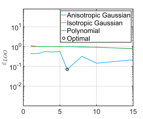
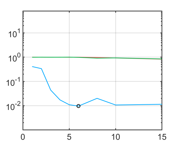
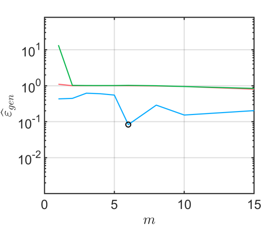
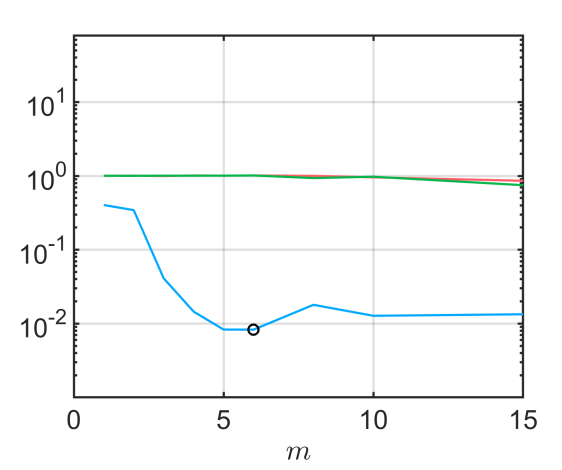
The DRSM algorithm identifies the anisotropic Gaussian kernel as the best KPCA kernel to be used in conjunction with both Kriging and PCE. However, the performance of PCE is significantly better in terms of generalisation error. The optimal parameters for each case (Kriging and PCE) are highlighted by a black dot in Figure 1, and their numerical values are reported in Table 1.

Table 1: Sobol’ function: optimal DRSM configurations for Kriging- and PCE-based surrogate models

SM method	KPCA kernel	$\widehat{m}$	$\varepsilon_{LOO}$	$\widehat{\varepsilon}_{gen}$
Kriging	Anisotropic Gaussian	$6$	0.0704	0.0830
PCE	Anisotropic Gaussian	$6$	0.0096	0.0083

Subsequently, the performance of DRSM is compared against an unsupervised approach, in which dimensionality reduction is carried out first, before applying surrogate modelling. To facilitate a meaningful comparison between the various methods, the reduced dimension and the optimal KPCA kernel as determined by the first analysis (see Table 1) is used. The results are summarised in Figure 2, while the corresponding list of tested configurations for both DRSM and the sequential DR-SM is given in Table 2.

Table 2: Different setups considered for evaluating the final surrogate model performance after using each of them for dimensionality reduction.

Dim. reduction	Parameter tuning objective	Abbreviation
Kernel PCA	$\varepsilon_{LOO}$ of Kriging (KG) or PCE surrogate (Eq. (13))	DRSM
Kernel PCA	Reconstruction error (Eq. (30))	KPCA-RECON
Kernel PCA	Pairwise distance preservation (Eq. (26))	KPCA-DIST
PCA	-	PCA

The experimental design consists of $800$ samples. The performance of each method is evaluated in terms of the generalisation error of the final surrogate $\widehat{{\mathcal{M}}}(\textbf{z})$ evaluated on a validation set $\left\{{\mathcal{X}}_{v},{\mathcal{Y}}_{v}={\mathcal{M}}({\mathcal{X}}_{v})\right\}$ with $10^{5}$ samples. To evaluate the robustness of the results, this process is repeated $10$ times, each corresponding to a different set ${\mathcal{X}}$, drawn at random using the Latin Hypercube sampling method. On the left (resp. right) panel, a Kriging (resp. PCE) surrogate is calculated using one of the methods in Table 2. Each box plot in Figure 2 provides summary statistics of the generalisation error that was achieved by each configuration over the $10$ repetitions. The central mark indicates the median, and the bottom and top edges of the box indicate the $25^{\text{th}}$ and $75^{\text{th}}$ percentiles, respectively. The whiskers extend to the most extreme data points up to $1.5$ times the inter-quartile range above or below the box edges. Any sample beyond that range is considered an outlier and plotted as a single point.

(a) Kriging

(b) Polynomial chaos expansions

Figure 2: Sobol’ function: estimates of the generalisation error with different DR approaches (see Table 2 for their description). The reduced dimension identified by DRSM (see Table 1) is used for all cases.

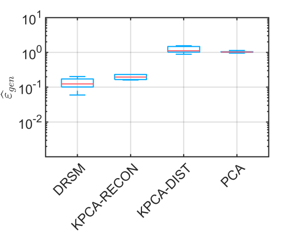
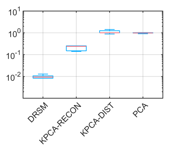
The DRSM approach consistently shows superior performance compared to the unsupervised approaches. This performance improvement becomes more apparent in the case of PCE surrogate modelling, where the average validation error over the $10$ repetitions is reduced by almost two orders of magnitude compared to the other methods. Further investigation on the significant performance difference between Kriging- and PCE- based DRSM shows that it stems from a combination of two different factors. On the one hand PCE models tend to achieve a lower generalization error than the corresponding Kriging models, regardless on the specific KPCA parameters on this particular function. On the other hand, the choice of a Kriging proxy surrogate with an isotropic covariance function causes the optimization in Eq. (14) to identify a sub-optimal configuration.

Due to the analytical nature of the model under consideration, we further evaluate the DRSM-based input compression by means of how the most important input variables are mapped to the reduced space. We adopt the total Sobol’ sensitivity indices as a rigorous measure of the importance of each input variable. Sobol’ sensitivity analysis is a form of global sensitivity analysis based on decomposing the variance of the model output into contributions that can be directly attributed to inputs or sets of inputs [57]. The total Sobol’ sensitivity index of an input variable $X_{i}$, denoted by $S_{i}^{Tot}\in[0,1]$, quantifies the total effect of $X_{i}$ on the variance of $Y$. In this particular example, the total Sobol’ indices can be analytically derived [53]. Their values are shown for reference in Figure 3(a).

(a) Total Sobol’ indices

(b) $m=3$

(c) $m=4$

(d) $m=5$

(e) $m=6$

Figure 3: Sobol’ function: total Sobol’ indices (in logarithmic scale) and visualisation of the sample-based Spearman correlation coefficient (absolute value) between the model inputs X and the reduced space inputs Z for varying reduced space dimension.

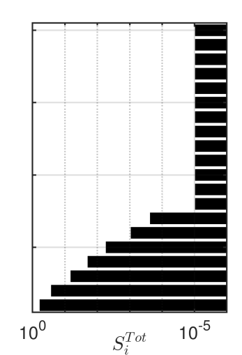
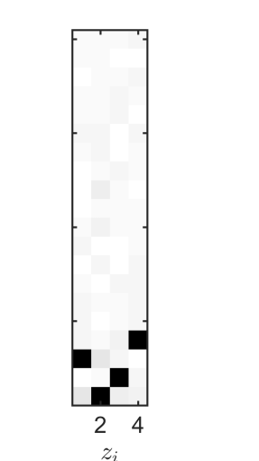
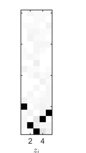
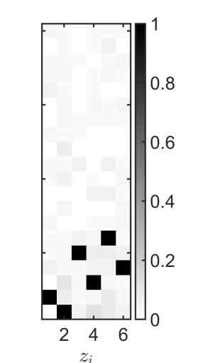
It is clear from Eq. (56) and Eq. (57) that all $20$ input variables contribute to the output variability, i.e. the intrinsic dimension of the problem is $20$. However, the contribution of each input component quickly diminishes with larger values of $c_{i}$ (see Figure 3(a) in which the values of the $20$ total Sobol’ indices are plotted, in logarithmic scale, as horizontal bars). Compressing the inputs in this problem is expected to lead to a mapping where those first few input components have the largest contribution.

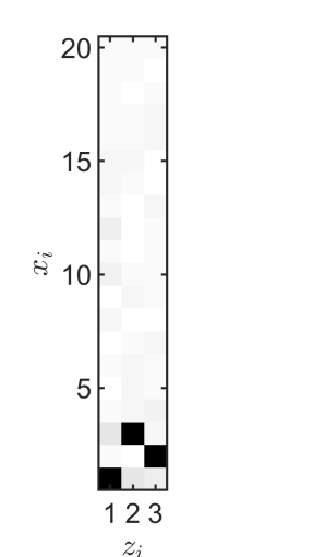
In Figure 3 the features in the reduced space Z are compared against the original inputs X. The rationale behind this heuristic analysis is simple: if the features obtained by DRSM are correctly identified, they should depend mostly on the same variables identified as important in the Sobol’ analysis in Figure 3(a). A simple measure of dependence between the reduced space components $\left\{z_{i}\,,\,i=1,\,\dots\,,m\right\}$ and the initial input space components $\left\{x_{i}\,,\,i=1,\,\dots\,,M\right\}$ is provided by the metric $\left|\rho\left(z_{i},x_{i}\right)\right|$, where $\rho$ denotes the Spearman correlation coefficient. Figures 3(b) - 3(e) represent graphically the quantity $\left|\rho\left(z_{i},x_{i}\right)\right|$ for the best surrogate identified in Table 1, namely a PCE coupled with KPCA using an anisotropic Gaussian kernel, evaluated on the validation set $\left\{{\mathcal{X}}_{v},{\mathcal{Y}}_{v}\right\}$. Each figure corresponds to a different selection of reduced space dimension $m$. Figure 3 clearly shows that (i) each $z_{i}$ correlates strongly with a specific $x_{i}$, (ii) the $z_{i}$’s correlate with the $m$ “most important” $x_{i}$’s, and, (iii) the larger $m$ value leads to the discovery of a new input $z_{i}$ that correlates with the next “most important” component of x.

(a) Kriging

(b) Polynomial chaos expansions

Figure 4: Sobol’ function: Optimal reduced space dimension (identified by DRSM) and generalisation error of the surrogate using an experimental design of varying size.

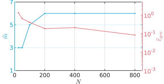
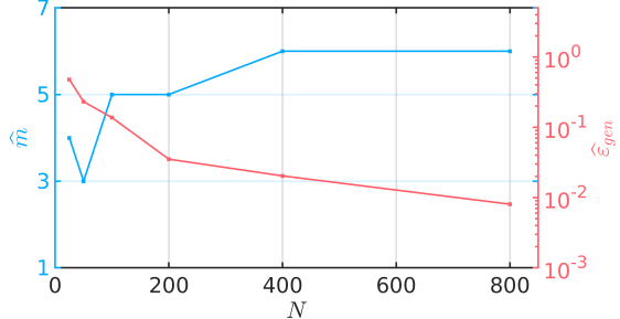
Finally, in Figure 4 we investigate the convergence behaviour of the DRSM algorithm, with respect to the experimental design size $N$. Using the same validation set as before, we repeat the DRSM training process using a varying number of samples in the experimental design. Figure 4(a) (resp. Figure 4(b)) shows the resulting generalisation performance of the Kriging (resp. polynomial chaos expansion) surrogate and the optimal reduced space dimension $\widehat{m}$ in each case. At a first glance, the convergence behaviour is similar when a Kriging or a PCE surrogate is used, but the latter shows consistently better performance regardless of the number of experimental design samples available. As expected, the identified optimal reduced dimension increases with the number of available experimental design points, plateauing in both cases to $\widehat{m}=6$. This is consistent with the notion that identifying the inherent dimensionality of a system requires a sufficient amount of information, which in this case is directly related to the available number of samples.

5.2 Electrical resistor network

Figure 5: The resistor networks application example

The electrical resistor network in Figure 5 [32] is considered next. It contains $80$ resistances of uncertain ohmage (model inputs) and it is driven by a voltage source providing a known potential $V_{0}$. The output of interest is the voltage $V$ at the node shown in Figure 5. A single set of $1,000$ experimental design samples and model responses is available, courtesy of J. Jakeman.

As in the previous section, the goal of the first analysis is to determine the generalisation performance of the DRSM surrogate as a function of the reduced space dimension $m$ when KPCA is combined with either Kriging or PCE. In addition, the accuracy of the LOO error in Eq. (10) is compared to the validation error in Eq. (7). The samples are randomly split into $500$ pairs $\left\{{\mathcal{X}},{\mathcal{Y}}\right\}$ used during the DRSM calibration and $500$ pairs $\left\{{\mathcal{X}}_{v},{\mathcal{Y}}_{v}\right\}$ used for validation.

(a) Kriging - LOO error

(b) PCE - LOO error

(c) Kriging - Validation error

(d) PCE - Validation error

Figure 6: Electrical resistor networks: error estimates of the DRSM surrogate as a function of the reduced dimension. Kernel PCA is used with anisotropic (resp. isotropic) Gaussian as well as polynomial kernels.

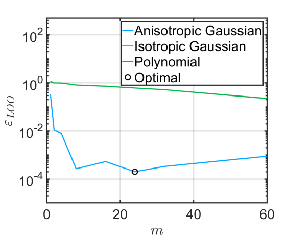
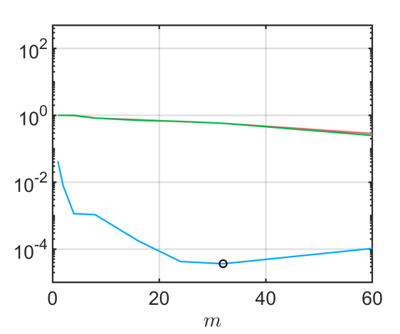
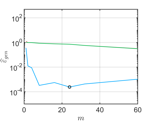
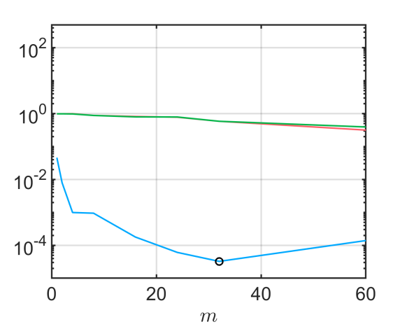
Figures 6(a) and 6(b) show the LOO error estimator of the final surrogate model (Kriging or PCE), evaluated on $\left\{{\mathcal{X}},{\mathcal{Y}}\right\}$, whereas Figures 6(c) and 6(d) show the validation error of the surrogate, evaluated on $\left\{{\mathcal{X}}_{v},{\mathcal{Y}}_{v}\right\}$. In each panel, each curve corresponds to a different KPCA kernel, namely anisotropic or isotropic Gaussian, and polynomial. Finally, the optimal configuration for each SM method is illustrated by a black dot. Similarly to the Sobol’ function, the use of an anisotropic kernel in KPCA results in significantly reduced generalisation error. Indeed this is expected from a physical standpoint. The effect of the resistors on the voltage $V$ will decay with distance (in terms of the number of preceding resistors) from $V$, which implies anisotropy in terms of the effect of each input variable to the output. As in the previous application example, the LOO error in Figures 6(a) and 6(b) provides a reliable proxy of the generalisation error in Figures 6(c) and 6(d) and the same optimal parameters are identified w.r.t. the two error measures. The optimal DRSM configuration for each surrogate model is given in Table 3.

Table 3: Resistor networks: optimal DRSM configurations for Kriging and PCE surrogate models

SM method	KPCA kernel	$\widehat{m}$	$\varepsilon_{LOO}$	$\widehat{\varepsilon}_{gen}$
Kriging	Anisotropic Gaussian	$24$	2.000e-04	2.402e-04
PCE	Anisotropic Gaussian	$32$	3.621e-05	3.249e-05

(a) Kriging

(b) Polynomial chaos expansions

Figure 7: Electrical resistor networks: estimates of the generalisation error with different DR approaches (see Table 2 for their description). The optimal dimensionality identified by DRSM (see Table 3) is used for all configurations.

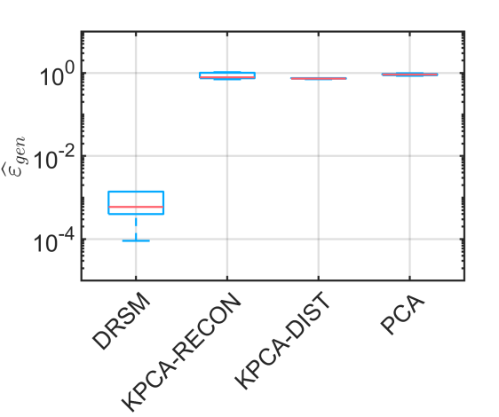
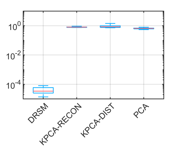
Next, the performance of DRSM is compared to unsupervised approaches considering the setups in Table 2. The results of this comparative study are given in Figure 7 using box plots. They are obtained by the repeated random selection of $500$ samples from the available $1,000$, leading to $10$ separate surrogate models for each case. The performance of each method is determined by means of the $\widehat{\varepsilon}_{gen}$ of the final surrogate $\widehat{{\mathcal{M}}}(\textbf{z})$ evaluated on the validation set $\left\{{\mathcal{X}}_{v},{\mathcal{Y}}_{v}={\mathcal{M}}({\mathcal{X}}_{v})\right\}$, that corresponds to the remaining $500$ samples of each split. Hence, each box-plot provides summary statistics of the validation error over the different splits. Each of the setups is tested both for Kriging (Figure 7(a)) and PCE surrogates (Figure 7(b)). In this application example the DRSM-based surrogates outperform the others by several orders of magnitude in both cases (Kriging, PCE). This highlights the difference between the unsupervised and supervised compression: compressing the input using only the information in ${\mathcal{X}}$ appears inefficient when followed by surrogate modelling.

(a) SRC coefficients

(b) $m=2$

(c) $m=4$

(d) $m=8$

(e) $m=16$

Figure 8: Electrical resistor networks: total Sobol’ indices (in logarithmic scale) and visualisation of the sample-based Spearman correlation coefficient (absolute value) between the model inputs X and the reduced space inputs Z for varying reduced space dimension.

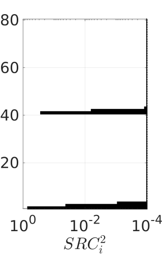
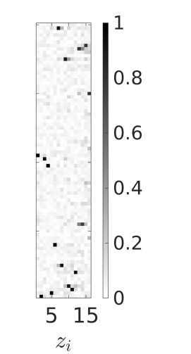
Finally, in Figure 8 we investigate how the reduced variables Z correlate with the input variables X. In contrast to the previous example, no computational model was available for this application, but only a relatively large pre-calculated dataset. To estimate the importance of each input variable in the physical space, we therefore chose to use a sensitivity measure called standardised regression coefficients (SRC, Helton et al. [25], Marelli et al. [40]). Standard regression coefficients correspond to the variance decomposition (Sobol’ indices) of a global linear model directly fitted on the available data:

$${\mathcal{M}}\left(\textbf{X}\right)\approx\beta_{0}+\sum_{i=1}^{M}\beta_{i}X_{i}\,,$$ (58)

where the coefficients $\bm{\beta}=\left\{\beta_{0},\,\dots\,,\beta_{M}\right\}$ are estimated by ordinary least-squares directly on the experimental design:

$$\widehat{\bm{\beta}}=\left({\mathcal{X}}^{\top}{\mathcal{X}}\right)^{-1}{\mathcal{X}}^{\top}{\mathcal{Y}}\,.$$ (59)

The SRC indices are then defined as:

$$SRC_{i}=\frac{\widehat{\bm{\beta}}\,\widehat{\sigma}_{X_{i}}}{\widehat{\sigma}_{Y}}\leavevmode\nobreak\ ,\leavevmode\nobreak\ i=1,\,\dots\,,M\,,$$ (60)

where $\widehat{\sigma}_{i}$ denotes the sample-based standard deviation of $X_{i}$ and ${\widehat{\sigma}_{Y}}$ the sample-based standard deviation of $Y$.

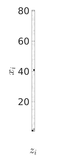
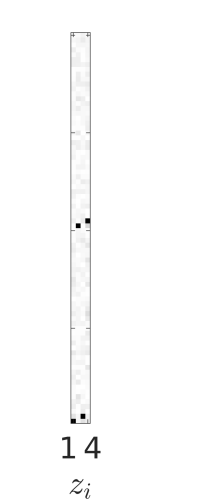
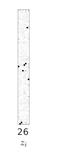
Their computational efficiency and simple interpretation (especially for linear- or quasi-linear models) are attractive, and little or no information about the input distributions is available. Because $\sum_{i=1}^{M}SRC_{i}^{2}\approx 1$, in Figure 8(a) we plot the $SRC_{i}^{2}$. Indeed variables $X_{1}$, $X_{2}$, $X_{41}$ and $X_{42}$ are expected to have the most significant contribution to the output variance because the effect of each resistor decays as the distance from $V$ increases. Similarly to case of the Sobol’ function, Figures 8(b) - 8(e) represent graphically the Spearman’s correlation coefficient $|\rho\left(z_{i},x_{i}\right)|$, each panel corresponding to a reduced space of different dimension. In each case, we used the DRSM algorithm to calculate the parameters of the KPCA (anisotropic Gaussian) kernel coupled with a PCE surrogate, because this setup performed best in Table 3. Interestingly we observe that as the dimensionality of the reduced space, $m$, increases, the most important variables $X_{i}$ are always captured by at least one $Z_{i}$, while the additional $Z_{i}$’s either correlate with the next more important input variable or correlate with multiple $X_{i}$’s when $m=8$ or larger.

When including the PCE prediction error results in Figures 6(b) and 6(d) in the picture, it is clear that the steep decline in the PCE generalisation error for $m<4$ is due to the importance of each of the four $X_{i}$’s with $i\in\left\{1,2,41,42\right\}$. For $4<m\leq 32$ the PCE accuracy still improves but at a reduced rate, because the additional $Z_{i}$’s still introduce further meaningful information about $Y$.

5.3 2-dimensional heat diffusion

As a last application, we consider a 2-dimensional stationary heat diffusion problem. The problem is defined in a square domain, $D=[-0.5,0.5]\times[-0.5,0.5]$, where the temperature field $T(\textbf{v}),\,\textbf{v}\in D$ is the solution of the elliptic partial differential equation:

$$-\nabla\cdot\left(d(\textbf{v})\nabla{}T(\textbf{v})\right)=500\,I_{A}(\textbf{v}),$$ (61)

with boundary conditions $T=0$ on the top boundary and $\nabla T\cdot\bm{n}=0$ on the left, right and bottom boundaries, where $\bm{n}$ denotes the vector normal to the boundary. In Eq. (61), $A$ corresponds to a square domain (see Figure 9) and $I_{A}$ is the indicator function equal to 1 if $\textbf{v}\in A$ and $0$ otherwise. The high dimensional input is given by the uncertain diffusion coefficient $d(\textbf{v})$. To generate samples of the diffusion coefficient, we choose to model it as a lognormal random field, defined by:

$$d(\textbf{v})=\exp\left(a_{d}+b_{d}\,g(\textbf{v})\right),$$ (62)

where $g(\textbf{v})$ is a Gaussian random field and the parameters $a_{d}$, $b_{d}$ are such that the mean and standard deviation of $d$ are $\mu_{d}=1$ and $\sigma_{d}=0.3$ respectively. The random field is characterised by a Gaussian correlation function $R(\textbf{v},\textbf{v}^{\prime})=\exp\left(-\left\lVert\textbf{v}-\textbf{v}^{\prime}\right\rVert^{2}/\ell^{2}\right)$, with $\ell=0.2$. The output of interest is the average temperature in the square domain $B$ within $D$ (see Figure 9).

(a) Finite element mesh

(b) Input random field realisation

(c) Corresponding temperature distribution

Figure 9: 2D heat diffusion problem: illustration of the model input and output.

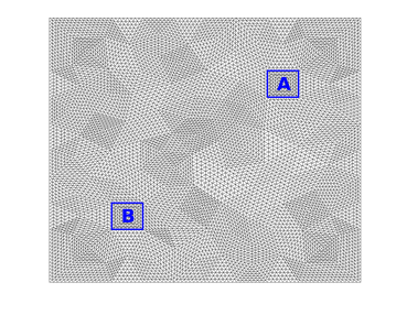
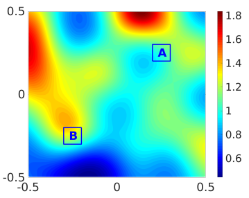
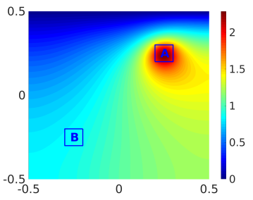
The underlying deterministic problem is solved with an in-house finite-element analysis code developed in Matlab. The mesh shown in Figure 9(a) consists of $16,000$ triangular T3 elements. Figure 9(b) shows a realisation of the diffusion coefficient random field which corresponds to the input of the model. The corresponding model output, shown in Figure 9(c), is the mean temperature in the highlighted square region $B$. Each realisation of the diffusion coefficient random field is discretised over the mesh in Figure 9(a). In the following analysis, the system is treated as a black-box, with the discretised heat diffusion coefficient as a high-dimensional input ($M=16,000$) and the average temperature in square B as the scalar model output. Realizations of the Gaussian random field $g(\textbf{v})$ are obtained on the modelling mesh with the expansion optimal linear estimation (EOLE) method [39], by retaining $p=30$ modes in the numerical expansion. A single set of $500$ experimental design samples and model responses is generated and made available for the analysis. This example mimics a realistic scenario in which various maps of spatially varying parameters measured on a regular grid are input to a computational model that analyses some performance of the system.

(a) Kriging - LOO error

(b) PCE - LOO error

(c) Kriging - Validation error

(d) PCE - Validation error

Figure 10: 2D heat diffusion problem: Error estimates of the DRSM surrogate as a function of the reduced space dimension. Kernel PCA is used with isotropic Gaussian and polynomial kernels.

Table 4: 2D diffusion: optimal DRSM configurations for Kriging- and PCE-based surrogate models

SM method	KPCA kernel	$\widehat{m}$	$\widehat{\textbf{w}}$ (Eq. (24))			$\varepsilon_{LOO}$	$\widehat{\varepsilon}_{gen}$
			$\widehat{w}_{1}$	$\widehat{w}_{2}$	$\widehat{w}_{3}$
Kriging	Polynomial	$20$	$131.3681$	$112.0040$	$1$	$0.0205$	$0.0216$
PCE	Polynomial	$20$	$17.5225$	$15.1853$	$1$	$0.0340$	$0.0356$

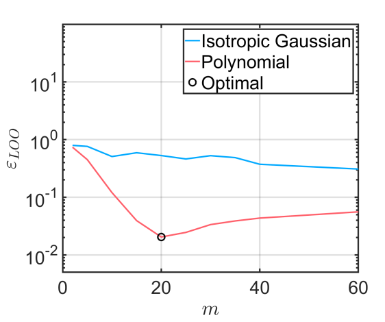
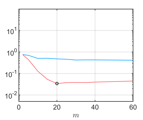
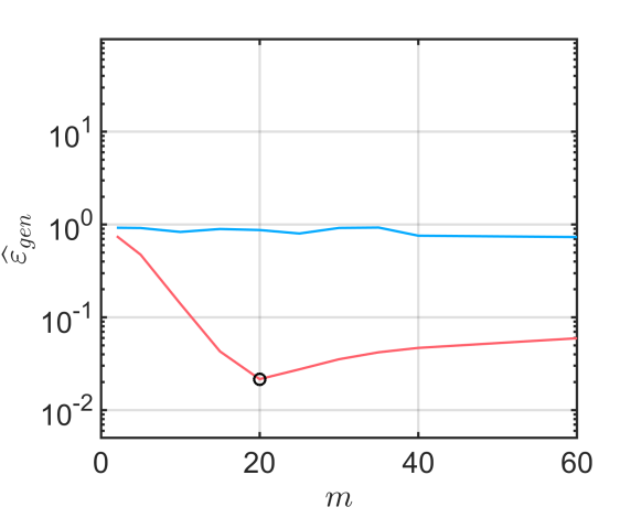
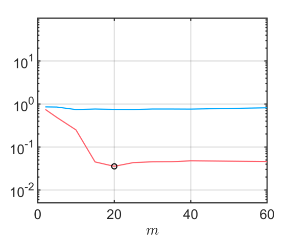
As in the previous application examples, the goal of the first analysis is to determine the optimal DRSM configuration in terms of the KPCA kernel and the reduced space dimension, as well as test the effectiveness of the LOO error as a proxy of the validation error. In this analysis, the available samples are randomly split into $300$ pairs to be used during the DRSM optimisation and $200$ pairs to be used for validation. The results are shown in Figure 10. Figures 10(a) and 10(b) show the LOO error estimator of the final Kriging (resp. PCE) surrogate, evaluated on $\left\{{\mathcal{X}},{\mathcal{Y}}\right\}$, whereas Figures 10(c) and 10(d) show the validation error of the surrogate evaluated on $\left\{{\mathcal{X}}_{v},{\mathcal{Y}}_{v}\right\}$. Each curve corresponds to a specific type of KPCA kernel, namely isotropic Gaussian and polynomial, and a specific surrogate, namely Kriging and PCE. We omitted the anisotropic Gaussian kernel for KPCA which is intractable due to the large input dimensionality.

A similar convergence behaviour is observed between Kriging- and PCE- based DRSM. The corresponding optimal parameter values are highlighted in Figure 10 and their numerical values are reported in Table 4. The linear polynomial kernel performs best in both cases and leads to the same reduced space dimension $\widehat{m}=20$. The convergence to a linear kernel is not surprising, as it corresponds to a re-scaled PCA (see A), which is in turn closely related to its KL expansion. This significantly low dimension has a twofold explanation: although $16,000$- dimensional, the heat diffusion coefficient is a non-linear combination of $p=30$ independent standard normal random variables (the modes retained in the EOLE expansion during the sampling procedure). Additionally, the forward operator in Eq. (61) has a smoothening effect that is captured by DRSM, further reducing the effective dimensionality of the problem. Moreover, the LOO and validation error curves show similar behaviour both in terms of their trend and their absolute value. Hence, the LOO error served as a reliable proxy of the validation error, as was observed in the previous application examples too.

(a) Kriging

(b) Polynomial chaos expansions

Figure 11: 2D heat diffusion problem: estimates of the generalisation error with different DR approaches (see Table 2 for their description). The optimal reduced dimension identified by DRSM (see Table 4) is used in all cases.

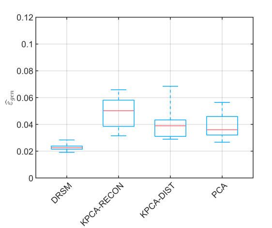
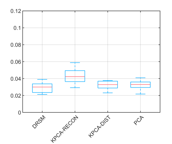
In the subsequent analysis we compare the performance of the DRSM approach against other sequential approaches listed in Table 2. To test each setup, we repeat the calculation process $10$ times. In each case the $500$ available samples are split randomly into $300$ samples for calculating the surrogate and $200$ samples for validation. The optimal KPCA kernel that was determined by DRSM is used in all methods that involve KPCA. Also, for the sake of comparison, the same reduced space dimension $\widehat{m}=20$ is assumed for all methods.

The results of this comparative study are given in Figure 11 using box plots to provide summary statistics of the validation error over the different splits of the samples. In case of Kriging surrogate modelling, DRSM consistently provides superior results compared to the other methods. The Kriging surrogates, in contrast to the PCE ones, are affected by this scaling. This also explains the performance improvement compared to the case of PCA-based DR. In case of PCE surrogate modelling, the performance improvement gained by DRSM is marginal compared to PCA and KPCA with distance preservation- based tuning of w.

Overall, DRSM consistently provides more accurate or at least comparable results compared to the other approaches. The main difference with a standard UQ setting in which the thermal conductivity is supposed to be sampled from a random field with known properties, is that the proposed DRSM methodology is purely data-driven, i.e. it would be applied identically in a case when the input maps are given without knowing the underlying random process.

6 Summary and Conclusions

Surrogate modelling is a key ingredient of modern uncertainty quantification. Due to the detrimental effects of high input dimensionality on most recent surrogate modelling techniques, the input space needs to be compressed to make such problems tractable. We proposed a novel approach for effectively combining dimensionality reduction with surrogate modelling, called DRSM. DRSM consists of three steps: (i) the DR and SM parameters are calculated by solving a nested optimisation problem, where only low-accuracy surrogates are considered to reduce the associated computational cost, (ii) the optimal configuration parameters, including the dimension of the reduced space, are empirically estimated based on the surrogate model performance, and, (iii) a final high-accuracy surrogate is calculated using the optimal values of all the aforementioned parameters.

The performance of DRSM was compared on three different benchmark problems of varying complexity against the classical approach of tuning the dimensionality reduction and surrogate modelling parameters sequentially. DRSM consistently showed superior performance compared to the others in all the benchmark applications.

The novelty of the proposed methodology lies in its non-intrusive way of combining dimensionality reduction and surrogate modelling. This allows for the combination of various techniques without the need of altering the dedicated optimisation algorithms on which each of them capitalises. A practical implication of the non-intrusiveness of DRSM is that off-the-shelf surrogate modelling methods (or even software) with sophisticated calibration algorithms can be directly used within this framework.

The focus was given to data-driven scenarios where only a limited set of observations and model responses is available. We demonstrated that the leave-one-out cross-validation error of the surrogate models can serve as a reliable proxy for estimating the generalisation error in order to tune the DR parameters, but also to assess the overall accuracy of the resulting surrogate.

In application-driven scenarios where the goal is to obtain a surrogate with optimal performance (regardless of its type) for that specific problem, the proposed approach could be extended in a way that the surrogate type itself is included as one of the parameters that DRSM needs to optimise. However, special care would need to be given to the error metric used during the DRSM optimisation in this case, because the LOO error estimations by different surrogates may have widely varied levels of bias (see e.g. Tibshirani and Tibshirani [59]).

In future extensions of this work, focus will be given to capitalising on available HPC resources to optimise for different combinations of surrogate models and dimensionality reduction methods. The choice of optimal low-accuracy surrogates needs also further study, as it may sometimes lead to relatively poor performance (e.g. as in the case of Kriging in Section 5.1). In addition, the cost of training surrogate models increases with the number of available experimental design samples. Therefore, research efforts will also be directed towards dealing with large experimental designs, possibly within a big data framework.

Appendix A Relationship between PCA and KPCA with linear kernel

Consider the PCA-based dimensionality reduction $\textbf{x}\in{\mathbb{R}}^{M}\mapsto\textbf{z}\in{\mathbb{R}}^{m}$. As discussed in Section 4.1, z is calculated as follows:

$$\textbf{z}=\textbf{x}^{\top}\bm{V},$$ (63)

where $\bm{V}\in{\mathbb{R}}^{M\times m}$ is the collection of the $m$ eigenvectors of $\bm{C}=\text{cov}\left[{\mathcal{X}}\right]$ and ${\mathcal{X}}\in{\mathbb{R}}^{N\times M}$ is the experimental design.

Next, consider the kernel PCA mapping $\textbf{x}\in{\mathbb{R}}^{M}\mapsto\bm{q}\in{\mathbb{R}}^{m}$ using the linear kernel function:

$$\kappa\left(\bm{x},\bm{x}^{\prime}\right)=a\,\bm{x}^{\top}\bm{x}^{\prime}+b.$$ (64)

It is straightforward to show that the following transformation is equivalent to the linear kernel in Eq. (64):

$$\Phi(\textbf{x})=\left\{\sqrt{b},\sqrt{a}\,x_{1},\,\dots\,,\sqrt{a}\,x_{M}\right\}^{\top},$$ (65)

because $\kappa\left(\bm{x},\bm{x}^{\prime}\right)=\Phi(\textbf{x})^{\top}\Phi(\textbf{x}^{\prime})$. A sample $\bm{q}$ in the reduced space is calculated as follows (see Section 4.2):

$$\bm{q}=\Phi(\textbf{x})^{\mathsf{T}}\bm{V}_{\mathcal{H}},$$ (66)

where $\bm{V}_{\mathcal{H}}$ is the collection of the $m$ eigenvectors of $\bm{C}_{{\mathcal{H}}}=\text{cov}\left[\Phi({\mathcal{X}})\right]$ with maximal eigenvalues. Notice that in case of $a=1$ and $b=0$, from Eqs. (63), (66) follows that $\textbf{z}=\bm{q}$.

The covariance matrix $\bm{C}_{{\mathcal{H}}}$ can be expressed as:

$$\bm{C}_{{\mathcal{H}}}=\begin{bmatrix}0&\ldots&0\\ \vdots&\lx@intercol\hfil\hbox{\multirowsetup$a\,\bm{C}$}\hfil\lx@intercol\\ 0\end{bmatrix}.$$ (67)

Hence, excluding the eigenvector that corresponds to the zero eigenvalue, it is straightforward to show that

$$\bm{V}_{{\mathcal{H}}}=\begin{bmatrix}0&\ldots&0\\ \lx@intercol\hfil\bm{V}\hfil\lx@intercol\\ \end{bmatrix}.$$ (68)

Based on Eqs. (65) and (68), Eq. (66) can be written as follows:

$$\bm{q} =\begin{bmatrix}\sqrt{b}&\sqrt{a}\,\textbf{x}^{\top}\end{bmatrix}\begin{bmatrix}0&\ldots&0\\ \lx@intercol\hfil\bm{V}\hfil\lx@intercol\\ \end{bmatrix}$$ (69)

$$=\sqrt{a}\,\textbf{x}^{\top}\bm{V}$$ (70)

$$=\sqrt{a}\,\textbf{z}\quad\text{(from Eq.\leavevmode\nobreak\ (\ref{eq:App_pca_z}))}$$ (71)

Therefore, the dimensionality reduction using kernel PCA with a linear kernel provides a scaled version of standard PCA and the constant $b$ has no effect.

Appendix B Implementation details

This section provides an extensive list of the configuration parameter values that were used to produce the results in Section 5. Table 5 (resp. Table 7)lists the configuration parameters of Kriging (resp. polynomial chaos expansions) surrogate models. For each surrogate method a distinction is made, in terms of the parameters used, between the proxy (i.e. low computational cost) surrogate and the high-accuracy one. The proxy surrogates were used for solving the nested optimisation problem of DRSM in Eqs. (13), (14). The same configuration was used to calculate the high-accuracy surrogates regardless of the input compression method (DRSM or disjoint PCA/KPCA).

Table 5: The configuration of the Kriging surrogates that were calculated during the various steps of DRSM for each application example.

Application	Sobol’ function	Resistor networks	2D diffusion
1. Proxy surrogate configuration
Trend	constant ($P=0$)	linear ($P=1$)	linear ($P=1$)
Correlation family	isotropic Matérn (Eq. (35)) with $\nu=5/2$
Estimation method	Cross-validation (Eq. (46))
Optim. method	Genetic algorithm (GA) with BFGS (gradient based) refinement of final solution
Optim. constraints	$\bm{\theta}\in[0.01,100]$
Population size (GA)	$10$
Max. iterations:	$20$ for both GA and BFGS
2. High-accuracy surrogate configuration. Only the parameters that differ from the proxy surrogate configuration are listed
Correlation family	anisotropic Matérn with $\nu=5/2$
Population size (GA)	$20$
Max. iterations:	$50$ for both GA and BFGS

Table 6: The configuration of the PCE surrogates that were calculated during the various steps of DRSM for each application example

Application	Sobol’ function	Resistor networks	2D diffusion
1. Proxy surrogate configuration
Coeff. calculation method	Ordinary least squares [6]
Univariate polynomials family	Legendre
Hyperbolic truncation $q$ [7]	$0.75$	$0.50$	$0.65$
Polynomial degree (adaptive search range)	$[1,10]$	$[1,10]$	$[1,5]$
2. High-accuracy surrogate configuration. Only the parameters that differ from the proxy surrogate configuration are listed
Coeff. calculation method	Hybrid least angle regression [8]
Univariate polynomials family	Orthogonal to the probability density function of the input variables that is estimated by kernel-smoothing, using the Stieltjes procedure [19]
Hyperbolic truncation $q$ [7]	$0.75$
Polynomial degree (adaptive search range)	$[1,15]$

The parameters of the DRSM-based optimisation are listed in Table 9. Note that the exact same optimisation algorithm and parameters were used for optimising w w.r.t. the KPCA reconstruction and point-wise distance error in the box-plots used to compare the various approaches. The optimisation constraints differ from the ones reported in Table 9 when a polynomial kernel is used in KPCA, as in Eq. (24), for improved numerical stability of the solver. On top of the bound constraints reported in the table, that still apply for $w_{1}$ and $w_{2}$, the variable $w_{3}$ (degree) is constrained to integer values $1\leq w_{3}\leq 4$ instead. In addition, the following non-linear constraint is included:

$$w_{1}\textbf{x}^{\mathsf{T}}\textbf{x}^{\prime}+w_{2}>1.$$ (72)

Table 8: Parameters of the DRSM optimisation algorithm

Application	Sobol’ function	Resistor networks	2D diffusion
Optim. method	Genetic algorithm with BFGS (gradient based) refinement of final solution
Optim. constraints	$\textbf{w}\in[0.1,300]$
Population size(GA):	$20$ for isotropic KPCA kernels, $80$ for anisotropic	$20$ for isotropic KPCA kernels, $100$ for anisotropic	$20$ (only isotropic KPCA kernels were considered)
Max. iterations:	$80$ for both GA and BFGS	$150$ for both GA and BFGS	$80$ for both GA and BFGS

References

- Alam and Fukumizu [2014] Alam, M. A. and K. Fukumizu (2014). Hyperparameter selection in kernel principal component analysis. J. Comput. Sci. 10(7), 1139–1150.
- Arlot and Celisse [2010] Arlot, S. and A. Celisse (2010). A survey of cross-validation procedures for model selection. Stat. Surveys 4, 40–79.
- Bachoc [2013] Bachoc, F. (2013). Cross validation and maximum likelihood estimations of hyper-parameters of Gaussian processes with model misspecifications. Comput. Stat. Data Anal. 66, 55–69.
- Bazaraa et al. [2013] Bazaraa, M. S., H. D. Sherali, and C. M. Shetty (2013). Nonlinear programming: theory and algorithms. John Wiley & Sons.
- Bertsekas [1999] Bertsekas, D. P. (1999). Nonlinear programming. Athena scientific Belmont.
- Berveiller et al. [2006] Berveiller, M., B. Sudret, and M. Lemaire (2006). Stochastic finite elements: a non intrusive approach by regression. Eur. J. Comput. Mech. 15(1-3), 81–92.
- Blatman and Sudret [2010] Blatman, G. and B. Sudret (2010). An adaptive algorithm to build up sparse polynomial chaos expansions for stochastic finite element analysis. Prob. Eng. Mech. 25, 183–197.
- Blatman and Sudret [2011] Blatman, G. and B. Sudret (2011). Adaptive sparse polynomial chaos expansion based on Least Angle Regression. J. Comput. Phys 230, 2345–2367.
- Calandra et al. [2016] Calandra, R., J. Peters, C. E. Rasmussen, and M. P. Deisenroth (2016). Manifold Gaussian processes for regression. In Neural Networks (IJCNN), 2016 International Joint Conference on, pp. 3338–3345. IEEE.
- Camastra [2003] Camastra, F. (2003). Data dimensionality estimation methods: a survey. Pattern recognition 36(12), 2945–2954.
- Chevreuil et al. [2015] Chevreuil, M., R. Lebrun, A. Nouy, and P. Rai (2015). A least-squares method for sparse low rank approximation of multivariate functions. SIAM/ASA J. Uncer. Quant. 3(1), 897–921.
- Constantine et al. [2014] Constantine, P. G., E. Dow, and Q. Wang (2014). Active subspace methods in theory and practice: applications to kriging surfaces. SIAM Journal on Scientific Computing 36(4), A1500–A1524.
- Damianou and Lawrence [2013] Damianou, A. and N. Lawrence (2013). Deep Gaussian processes. In Artificial Intelligence and Statistics, pp. 207–215.
- Djolonga et al. [2013] Djolonga, J., A. Krause, and V. Cevher (2013). High-dimensional Gaussian process bandits. In Advances in Neural Information Processing Systems, pp. 1025–1033.
- Dubrule [1983] Dubrule, O. (1983). Cross validation of Kriging in a unique neighborhood. J. Int. Assoc Math. Geology 15(6), 687–699.
- Durrande et al. [2012] Durrande, N., D. Ginsbourger, and O. Roustant (2012). Additive covariance kernels for high-dimensional Gaussian process modeling. In Annales de la Faculté de Sciences de Toulouse, Volume 21, pp. p–481.
- Fornasier et al. [2012] Fornasier, M., K. Schnass, and J. Vybiral (2012). Learning functions of few arbitrary linear parameters in high dimensions. Foundations of Computational Mathematics 12(2), 229–262.
- Fukunaga [2013] Fukunaga, K. (2013). Introduction to statistical pattern recognition. Academic press.
- Gautschi [2004] Gautschi, W. (2004). Orthogonal Polynomials: Computation and Approximation. Numerical Mathematics and Scientific Computation. Oxford University Press.
- Ghanem and Spanos [1991] Ghanem, R. and P. Spanos (1991). Stochastic finite elements – A spectral approach. Springer Verlag, New York. (Reedited by Dover Publications, Mineola, 2003).
- Goldberg [1989] Goldberg, D. E. (1989). Genetic algorithms in search, optimization and machine learning. Addison-Wesley Longman Publishing Co., Inc.
- Gu and Berger [2016] Gu, M. and J. O. Berger (2016). Parallel partial Gaussian process emulation for computer models with massive output. The Annals of Applied Statistics 10(3), 1317–1347.
- Hansen et al. [2003] Hansen, N., S. D. Müller, and P. Koumoutsakos (2003). Reducing the time complexity of the derandomized evolution strategy with covariance matrix adaptation (cma-es). Evolutionary computation 11(1), 1–18.
- Hastie et al. [2001] Hastie, T., R. Tibshirani, and J. Friedman (2001). The elements of statistical learning: Data mining, inference and prediction. Springer, New York.
- Helton et al. [1985] Helton, J. C., R. L. Iman, and J. B. Brown (1985). Sensitivity analysis of the asymptotic behavior of a model for the environmental movement of radionuclides. Ecological modelling 28(4), 243–278.
- Hinton and Roweis [2003] Hinton, G. E. and S. T. Roweis (2003). Stochastic neighbor embedding. In Advances in neural information processing systems, pp. 857–864.
- Hinton and Salakhutdinov [2006] Hinton, G. E. and R. R. Salakhutdinov (2006). Reducing the dimensionality of data with neural networks. Science 313(5786), 504–507.
- Huang et al. [2015] Huang, W.-b., D. Zhao, F. Sun, H. Liu, and E. Y. Chang (2015). Scalable Gaussian process regression using deep neural networks. In IJCAI, pp. 3576–3582.
- Hyvärinen and Oja [1997] Hyvärinen, A. and E. Oja (1997). One-unit learning rules for independent component analysis. In Advances in neural information processing systems, pp. 480–486.
- Ince and Trafalis [2007] Ince, H. and T. B. Trafalis (2007). Kernel principal component analysis and support vector machines for stock price prediction. Iie Transactions 39(6), 629–637.
- Iooss and Lemaître [2015] Iooss, B. and P. Lemaître (2015). A review on global sensitivity analysis methods. In Uncertainty management in simulation-optimization of complex systems, pp. 101–122. Springer.
- Jakeman et al. [2015] Jakeman, J., M. Eldred, and K. Sargsyan (2015). Enhancing -minimization estimates of polynomial chaos expansions using basis selection. J. Comput. Phys. 289, 18–34.
- Kersaudy et al. [2015] Kersaudy, P., B. Sudret, N. Varsier, O. Picon, and J. Wiart (2015). A new surrogate modeling technique combining Kriging and polynomial chaos expansions – Application to uncertainty analysis in computational dosimetry. J. Comput. Phys 286, 103–117.
- Konakli and Sudret [2016a] Konakli, K. and B. Sudret (2016a). Global sensitivity analysis using low-rank tensor approximations. Reliab. Eng. Sys. Safety 156, 64–83.
- Konakli and Sudret [2016b] Konakli, K. and B. Sudret (2016b). Polynomial meta-models with canonical low-rank approximations: Numerical insights and comparison to sparse polynomial chaos expansions. J. Comput. Phys. 321, 1144–1169.
- Kwok and Tsang [2003] Kwok, J. T. and I. W. Tsang (2003). The pre-image problem in kernel methods. In Proc. 20th Int. Conf. Machine Learning (ICML-03), pp. 408–415.
- Lataniotis et al. [2018] Lataniotis, C., S. Marelli, and B. Sudret (2018). The Gaussian process modelling module in UQLab. Soft Comput. Civil Eng. 2(3), 91–116.
- Lawrence [2005] Lawrence, N. (2005). Probabilistic non-linear principal component analysis with Gaussian process latent variable models. J. Machine Learning Research 6, 1783–1816.
- Li and Der Kiureghian [1993] Li, C. and A. Der Kiureghian (1993). Optimal discretization of random fields. J. Eng. Mech. 119(6), 1136–1154.
- Marelli et al. [2019] Marelli, S., C. Lamas, K. Konakli, C. Mylonas, P. Wiederkehr, and B. Sudret (2019). UQLab user manual – Sensitivity analysis. Technical report, Chair of Risk, Safety & Uncertainty Quantification, ETH Zurich. Report # UQLab-V1.2-106.
- Marelli and Sudret [2014] Marelli, S. and B. Sudret (2014). UQLab: A framework for uncertainty quantification in Matlab. In Vulnerability, Uncertainty, and Risk (Proc. 2nd Int. Conf. on Vulnerability, Risk Analysis and Management (ICVRAM2014), Liverpool, United Kingdom), pp. 2554–2563.
- Marelli and Sudret [2018] Marelli, S. and B. Sudret (2018). UQLab user manual – polynomial chaos expansions. Technical report, Chair of Risk, Safety & Uncertainty Quantification, ETH Zurich. Report UQLab-V1.1-104.
- McKay et al. [1979] McKay, M. D., R. J. Beckman, and W. J. Conover (1979). A comparison of three methods for selecting values of input variables in the analysis of output from a computer code. Technometrics 2, 239–245.
- Mika et al. [1999] Mika, S., B. Schölkopf, A. J. Smola, K.-R. Müller, M. Scholz, and G. Rätsch (1999). Kernel pca and de-noising in feature spaces. In Advances in neural information processing systems, pp. 536–542.
- Moustapha et al. [2018] Moustapha, M., B. Sudret, J.-M. Bourinet, and B. Guillaume (2018). Comparative study of Kriging and support vector regression for structural engineering applications. ASCE-ASME J. Risk Uncertainty Eng. Syst., Part A: Civ. Eng. 4(2). Paper #04018005.
- Papaioannou et al. [2019] Papaioannou, I., M. Ehre, and D. Straub (2019). PLS-based adaptation for efficient PCE representation in high dimensions. Journal of Computational Physics 387, 186–204.
- Pearson [1901] Pearson, K. (1901). On lines and planes of closest fit to systems of points in space. Phil. Mag. 6(2), 559–572.
- Pedregosa et al. [2011] Pedregosa, F., G. Varoquaux, A. Gramfort, V. Michel, B. Thirion, O. Grisel, M. Blondel, P. Prettenhofer, R. Weiss, V. Dubourg, et al. (2011). Scikit-learn: Machine learning in python. J. Machine Learning Research 12(Oct), 2825–2830.
- Ramsay [2004] Ramsay, J. O. (2004). Functional data analysis. Encyclopedia of Statistical Sciences 4.
- Rasmussen and Williams [2006] Rasmussen, C. and C. Williams (2006). Gaussian processes for machine learning (Internet ed.). Adaptive computation and machine learning. Cambridge, Massachusetts: MIT Press.
- Roweis and Saul [2000] Roweis, S. T. and L. K. Saul (2000). Nonlinear dimensionality reduction by locally linear embedding. Science 290(5500), 2323–2326.
- Sacks et al. [1989] Sacks, J., W. Welch, T. Mitchell, and H. Wynn (1989). Design and analysis of computer experiments. Stat. Sci. 4, 409–435.
- Saltelli et al. [2000] Saltelli, A., K. Chan, and E. Scott (Eds.) (2000). Sensitivity analysis. J. Wiley & Sons.
- Saltelli et al. [2008] Saltelli, A., M. Ratto, T. Andres, F. Campolongo, J. Cariboni, D. Gatelli, M. Saisana, and S. Tarantola (2008). Global Sensitivity Analysis – The Primer. Wiley.
- Santner et al. [2003] Santner, T. J., B. J. Williams, and W. I. Notz (2003). The Design and Analysis of Computer Experiments. Springer New York.
- Schölkopf et al. [1998] Schölkopf, B., A. Smola, and K.-R. Müller (1998). Nonlinear component analysis as a kernel eigenvalue problem. Neural Comput. 10(5), 1299–1319.
- Sobol’ [1993] Sobol’, I. (1993). Sensitivity estimates for nonlinear mathematical models. Math. Modeling & Comp. Exp. 1, 407–414.
- Tenenbaum et al. [2000] Tenenbaum, J. B., V. De Silva, and J. C. Langford (2000). A global geometric framework for nonlinear dimensionality reduction. Science 290(5500), 2319–2323.
- Tibshirani and Tibshirani [2009] Tibshirani, R. J. and R. Tibshirani (2009). A bias correction for the minimum error rate in cross-validation. Ann. Applied Statistics, 822–829.
- Tipireddy and Ghanem [2014] Tipireddy, R. and R. G. Ghanem (2014). Basis adaptation in homogeneous chaos spaces. Journal of Computational Physics 259, 304–317.
- Torre et al. [2019] Torre, E., S. Marelli, P. Embrechts, and B. Sudret (2019). Data-driven polynomial chaos expansion for machine learning regression. J. Comp. Phys. 388, 601–623.
- Tsilifis et al. [2019] Tsilifis, P., X. Huan, C. Safta, K. Sargsyan, G. Lacaze, J. C. Oefelein, H. Najm, and R. G. Ghanem (2019). Compressive sensing adaptation for polynomial chaos expansions. Journal of Computational Physics 380, 29–47.
- Vapnik [1995] Vapnik, V. (1995). The Nature of Statistical Learning Theory. Springer-Verlag, New York.
- Verleysen and François [2005] Verleysen, M. and D. François (2005). The curse of dimensionality in data mining and time series prediction. In J. Cabestany, A. Prieto, and F. Sandoval (Eds.), Computational Intelligence and Bioinspired Systems, Volume 3512 of Lecture Notes in Computer Science, pp. 758–770. Springer Berlin Heidelberg.
- Vincent et al. [2008] Vincent, P., H. Larochelle, Y. Bengio, and P.-A. Manzagol (2008). Extracting and composing robust features with denoising autoencoders. In Proc. 25th Int. Conf. Machine learning, pp. 1096–1103. ACM.
- Wahlström et al. [2015] Wahlström, N., T. B. Schön, and M. P. Deisenroth (2015). Learning deep dynamical models from image pixels. IFAC-PapersOnLine 48(28), 1059–1064.
- Wang [2011] Wang, Q. (2011). Kernel principal component analysis and its applications in face recognition and active shape models. CoRR abs/1207.3538.
- Weinberger et al. [2004] Weinberger, K. Q., F. Sha, and L. K. Saul (2004). Learning a kernel matrix for nonlinear dimensionality reduction. In 21st Int. Conf. on Machine Learning, pp. 106. ACM.
- Weston et al. [2004] Weston, J., B. Schölkopf, and G. H. Bakir (2004). Learning to find pre-images. In Advances in neural information processing systems, pp. 449–456.
- Wilson et al. [2016] Wilson, A. G., Z. Hu, R. Salakhutdinov, and E. P. Xing (2016). Deep kernel learning. In Artificial Intelligence and Statistics, pp. 370–378.
- Xiu [2010] Xiu, D. (2010). Numerical methods for stochastic computations – A spectral method approach. Princeton University press.
- Xiu and Karniadakis [2002] Xiu, D. and G. E. Karniadakis (2002). The Wiener-Askey polynomial chaos for stochastic differential equations. SIAM J. Sci. Comput. 24(2), 619–644.
- Yang et al. [2007] Yang, Z., K. Tang, and X. Yao (2007). Differential evolution for high-dimensional function optimization. In Evolutionary Computation, 2007. CEC 2007. IEEE Congress on, pp. 3523–3530. IEEE.