Robust velocity dispersion and binary population modeling of the ultra-faint dwarf galaxy Reticulum II

Abstract

We apply a Bayesian method to model multi-epoch radial velocity measurements in the ultra-faint dwarf galaxy Reticulum II, fully accounting for the effects of binary orbital motion and systematic offsets between different spectroscopic datasets. We find that the binary fraction of Ret II is higher than 0.5 at the 90% confidence level, if the mean orbital period is assumed to be 30 years or longer. Despite this high binary fraction, we infer a best-fit intrinsic dispersion of 2.8${}_{-1.2}^{+0.7}$ km/s, which is smaller than previous estimates, but still indicates Ret II is a dark-matter dominated galaxy. We likewise infer a $\lesssim$ 1% probability that Ret II’s dispersion is due to binaries rather than dark matter, corresponding to the regime $M_{\odot/L_{\odot}}\lesssim$ 2. Our inference of a high close binary fraction in Ret II echoes previous results for the Segue 1 ultra-faint dwarf and is consistent with studies of Milky Way halo stars that indicate a high close binary fraction tends to exist in metal-poor environments.

1. Introduction

Ultra-faint dwarf (UFD) galaxies comprise the extreme end of the galaxy luminosity function, being the faintest and most dark matter dominated galaxies known. Their high mass-to-light ratios (Simon & Geha, 2007), paucity of gas and extremely low metallicities (Kirby et al., 2008) indicate they host very old and sparse star populations, with the bulk of their star formation occurring before the epoch of reionization and being quenched not long after (Brown et al., 2012). As a result of their high dark matter content, UFD’s are excellent laboratories for understanding the nature of dark matter in several respects: their expected abundance and density profile depends sensitively on the particle nature of dark matter, for example if it is warm (Lovell et al., 2014) or has a significant cross-section for self-interactions (Elbert et al., 2018; Rocha et al., 2013). In addition they are excellent targets to search for the products of dark matter self-annihilation, as a result of their low astrophysical backgrounds (Ackermann et al., 2015). The study of UFD’s has been reinvigorated in the past few years by the recent discovery of several new candidate dwarf galaxies by the Dark Energy Survey (Bechtol et al., 2015; Koposov et al., 2015a; Drlica-Wagner et al., 2015; Kim & Jerjen, 2015; Luque et al., 2016, 2017b, 2017a).

The estimated high dark matter content of ultra-faint dwarf galaxies hinges on an accurate measurement of the line-of-sight velocity dispersion of their constituent stars, with dispersions typically in the range of 1-6 km/s (Simon & Geha, 2007). However, their low intrinsic dispersions make the task difficult for a few reasons. First, in many cases they are too distant for radial velocities of main sequence stars to be measured by present instruments, leaving only the red giants in the sample. Second, spectrographs have systematic floors which limit the measurement of stellar velocities to greater than $\sim 0.2-2.2$ km/s. Finally, the dispersions are low enough that the orbital motion of close binary systems can inflate them significantly (Spencer et al., 2017; McConnachie & Côté, 2010; Wilkinson et al., 2002).

Of these systematics, binaries are perhaps the most worrisome, because unexpectedly high radial velocity variations have been detected in several UFD’s. This occurred, for example, among RGB stars in the Segue 1 sample, which did not inflate its dispersion dramatically due to a large sample of main sequence turnoff stars (Simon et al., 2011). An initial velocity dispersion measurement of Triangulum II (Kirby et al., 2015; Martin et al., 2016) had 1-2 unresolved binaries that inflated its dispersion (Kirby et al., 2017). Similarly, the dispersion of Boötes II (Koch et al., 2009) is inflated due to a known binary (Ji et al., 2016b), and Carina II’s dispersion would likely have been inflated if multi-epoch spectroscopy had not been obtained (see one epoch row of Table 3 in Li et al., 2018). In classical dwarf spheroidals, measured binary fractions appear to vary considerably, with some being higher and others lower than the exected value for Milky Way field binaries (Minor, 2013; Spencer et al., 2017; Olszewski et al., 1996). Besides dwarf galaxies, within the Milky Way there is mounting evidence that the fraction of close binaries is indeed higher in low metallicity systems (Moe et al., 2018; Badenes et al., 2018). Thus, there is a very real possibility that the measured dispersions of many ultra-faint dwarfs are significantly inflated due to binary motion; indeed, some may turn out to be diffuse globular clusters in disguise.

The most direct way to correct the dispersions of UFD’s for binary motion is to perform spectroscopic follow-up over two or more epochs, and model the binary contribution to the radial velocities directly. This strategy was carried out in the case of Segue 1 (Simon et al., 2011; Martinez et al., 2011). While spectroscopic follow-up has been recently performed for a few of the recent DES dwarfs, including Reticulum II, the binary modeling is complicated by the fact that radial velocity measurements have been made using different instruments and different methods of analysis (Simon et al., 2015; Koposov et al., 2015b; Ji et al., 2016b; Roederer et al., 2016). This gives rise to systematic velocity offsets between the different datasets which can masquerade as binary variability. As a result, any attempt to model the binary component of velocity variations should include systematic velocity offsets between datasets as model parameters.

In this paper we constrain the velocity dispersion of the ultra-faint dwarf Reticulum II, including the effects of binary orbital motion and systematic offsets between datasets, in a Bayesian analysis. By constructing the binary likelihood for each star and comparing it to the single-star likelihood, a probability of binarity can be inferred that does not rely on definitively identifying an individual star as a binary. The approach is similar to that employed for Segue 1, except that in addition we include systematic offset parameters to be inferred alongside the binary population parameters; hence, any degeneracy between the intrinsic dispersion, instrumental systematics, and binarity can be inferred in a consistent manner.

(a) S15 vs. K15

(b) J16 vs. S15, K15

Figure 1.— Comparison of velocity measurements between datasets for stars that are common to both datasets. The error bars represent 1-sigma errors for each dataset. The dashed line corresponds to equal velocities being measured, e.g. in (a) it represents $v_{S15}=v_{K15}$. Note that the S15 and K15 measurements are separated by only 18 days, and therefore binary orbital motion is unlikely to account for the majority of offsets between the two datasets in figure (a).

2. Bayesian Method: correcting for binaries

In order to correct the velocity dispersion of Reticulum II for binary orbital motion, we follow the method used in Martinez et al. (2011) and Minor (2013): we construct a multi-epoch likelihood for binary stars and use this to infer posterior probabilities in the galaxy kinematic parameters as well as parameters describing the binary population. Since this approach has been described in previous papers, we will give a brief summary here and describe the differences in our approach compared to previous papers.

Suppose a star of absolute magnitude $M$ has a set of $n$ velocity measurements $\{v_{i}\}=\{v_{1},\dots,v_{n}\}$ and errors $\{e_{i}\}$ taken at the corresponding dates $\{t_{i}\}$. For readability, when writing probability distributions we will suppress the brackets that denote sets of measurements (e.g., $P(\{v_{i}\})\rightarrow P(v_{i})$). Since the velocities at different epochs in the Ret II dataset were measured using different spectrographs, we will allow for each epoch to have a possible systematic velocity offset $\lambda_{i}$. Thus, our likelihood will be written in terms of the corrected velocities

$$v_{i}^{\prime}=v_{i}-\lambda_{i}.$$ (1)

For some epochs we will fix the corresponding systematic offsets to zero, while for others we will vary the offsets as free parameters. The set of systematic offsets to be varied will be denoted as $\mathcal{S}=\{\lambda_{1},\lambda_{2},\ldots\}$. Our velocity likelihood then becomes,

$$\mathcal{L}(v_{i}|e_{i},t_{i},M;\sigma,\mu,B,\mathcal{S})$$ (2)

$$~{}= ~{}(1-B)\mathcal{L}(\Delta v_{ij}^{\prime},e_{i})\frac{e^{-\frac{(\langle v^{\prime}\rangle-\mu)^{2}}{2(\sigma^{2}+e_{m}^{2})}}}{\sqrt{2\pi(\sigma^{2}+e_{m}^{2})}}~{}~{}~{}~{}~{}~{}~{}~{}~{}~{}~{}~{}~{}~{}~{}~{}$$

$$~{}~{}~{}~{}~{}~{}~{}~{}~{}~{}~{}~{}~{}~{}~{}~{}+~{}B\mathcal{L}_{b}(v_{i}|e_{i},t_{i},M;\sigma,\mu,\mathcal{S}),$$

where the first term gives the likelihood for non-binary stars, and the second is the binary star likelihood. Note that the non-binary likelihood has been factorized into a likelihood in the star’s mean velocity $\langle v^{\prime}\rangle$, and a likelihood in terms of velocity differences, denoted by $\mathcal{L}(\Delta v_{ij}^{\prime},e_{i})$; the latter is given by

$$\mathcal{L}(\Delta v_{ij}^{\prime},e_{i})~{}~{}=~{}~{}\frac{\sqrt{2\pi e_{m}^{2}}}{\prod_{i=1}^{n}\sqrt{2\pi e_{i}^{2}}}$$ (3)

$$\times \exp\left\{-\frac{1}{4}\sum_{i,j=1}^{n}\frac{(v_{i}^{\prime}-v_{j}^{\prime})^{2}}{e_{i}^{2}+e_{j}^{2}+e_{i}^{2}e_{j}^{2}\left(\sum_{k\neq i,j}\frac{1}{e_{k}^{2}}\right)}\right\}.$$

The last term in the denominator of the exponent is implicitly zero when $n=2$. To generate the likelihood for binary stars (the second term in equation 2), we first generate the binary likelihood in the center-of-mass frame of the binary system, denoted by $P_{b}(v_{i}^{\prime}-v_{cm}|e_{i},t_{i},M)$. This is done by running a Monte Carlo simulation where the binary properties are drawn from distributions similar to those observed in the solar neighborhood (see Minor et al. 2010 for details on the orbital parameters and their assumed distributions), and binning the resulting stellar velocities over a table of $v_{cm}$, $\lambda_{i}$ values. To ensure accuracy of the resulting likelihood, points are added to the bins until the binary likelihood (or rather, its integral over $v_{cm}$) converges to within a specified tolerance. For each likelihood evaluation, given values of the galaxy’s systemic velocity $\mu$ and dispersion $\sigma$, we interpolate in the offset parameters $\lambda_{i}$ and integrate over the tabulated $v_{cm}$ values as follows:

$$\mathcal{L}_{b}(\sigma,\mu,\mathcal{S})=\int_{-\infty}^{\infty}P_{b}(v_{i}^{\prime}-v_{\mathrm{cm}}|e_{i},t_{i},M)\frac{e^{-\frac{(v_{\mathrm{cm}}-\mu)^{2}}{2\sigma^{2}}}}{\sqrt{2\pi\sigma^{2}}}dv_{\mathrm{cm}}.$$ (4)

From a hierarchical modeling point of view, this can be thought of as marginalizing over $v_{cm}$ for each star, assuming a Gaussian prior whose hyperparameters $\mu$, $\sigma$ will be determined at the next level of inference (indeed, this has already been done implicitly for the nonbinary likelihood to give the Gaussian factor in eq. 2).

As in Martinez et al. (2011), we assume a log-normal period distribution for the binaries; however, we do not vary the period distribution parameters of the underlying binary population, since the constraints would be very poor given the sample size. However, for the sake of comparison we will test two models: one in which the period distribution is similar to Milky Way field binaries with a mean period of $\sim$180 years (Duquennoy & Mayor, 1991), and one in which the mean period is $10^{4}$ days $\approx$ 27 years. As we discuss in Section 4, the latter choice is motivated by the mean period inferred in low-metallicity halo stars in Moe et al. (2018). In both cases, the width of the log-period distribution is assumed to be $\sigma_{\log P}=2.3$, similar to that of binaries in the solar neighborhood as determined by Duquennoy & Mayor (1991) and independently by Raghavan et al. (2010).

3. Data

We make use of three different radial velocity datasets from Ret II, composed entirely of red giant stars with high probability of membership. The bulk of the velocity measurements come from Simon et al. (2015) using the Magellan/M2FS spectrograph (hereafter referred to as S15), of which 25 stars were identified as members, and Koposov et al. (2015b) using VLT/Giraffe with 18 member stars (hereafter K15). Nearly all of the stars in the K15 sample were also included in the S15 sample, with the observations were taken 18 days apart. Hence, only very short period binaries with periods less than a year can be expected to show significant velocity variations beyond the measurement error between these two datasets. We also include high-resolution velocity measurements of 9 member stars from Ji et al. (2016a) using the Magellan/MIKE spectrograph, along with four additional high-resolution measurements from Roederer et al. (2016) (hereafter J16/R16). Compared to the original S15 dataset, these later measurements occur 226 and 268 days later, respectively, so these stars may be expected to show velocity variations if they are binaries with periods of order a few years or shorter. Although we have only eleven stars with repeat measurements over timescales of several months, these latter measurements carry greater relative weight due to the small measurement errors ($\sim$ 0.1-0.2 km/s) in the J16/R16 datasets.

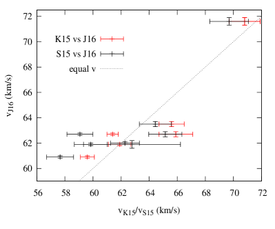
Since the stars in our sample have velocity measurements from multiple datasets using different spectrographs, any systematic offset between the datasets would bias the inferred binary fraction in our analysis. To guard against this, we will model such systematic offsets explicitly as free parameters. To get a sense of whether such offset(s) are present, in Figure 1(a) we plot a comparison of velocity measurements between the S15 and K15 datasets for stars that are common to both. Interestingly, most stars lie well above the line $v_{S15}=v_{K15}$, and in a few stars this difference is beyond $2\sigma$ for the measurement errors in either dataset. Since the measurements were taken only 18 days apart, this apparent offset in a large number of stars is unlikely to be explained by binary motion unless the binary population is quite extreme. The implication is that either the K15 data may have a positive systematic offset, S15 may have a negative offset, or perhaps some combination of the two. Likewise, in Figure 1(b) we compare the J16 measurements with S15 and K15. Since the measurements in this figure were taken 7-8 months apart, we may expect up to a few of the velocity differences to be due to binary motion. With this caveat in mind, a few stars in both S15 and K15 seem to have a positive velocity difference relative to J15 that lies beyond 2$\sigma$.

With this in mind, we will include offsets in S15 and K15 as free parameters. There is little to be gained by including an extra systematic offset parameter for the J16 and R16 measurements, because the systemic velocity of the galaxy is not known a priori; hence, an offset to all the measured velocities would simply translate the resulting mean velocity and thus there would be no unique solution for all the offsets and systemic velocity. If it turns out that J16 and R16 in fact have a systematic offset relative to S16 and K16, our analysis would result in a biased inferred systemic velocity, but otherwise this would not affect our inferred dispersion or binary fraction.

Figure 2.— Joint posteriors in the systemic velocity $v_{sys}$, intrinsic velocity dispersion $\sigma$, binary fraction $B$, the velocity offset in the K15 dataset $\lambda_{K15}$, and the relative offset $\Delta\lambda_{SK}=\lambda_{K15}-\lambda_{S15}$. In this analysis, the mean period of Ret II is assumed to be $10^{4}$ days ($\approx$ 27 years), with a spread in the log-normal period distribution identical to Milky Way field binaries $\sigma_{\log P}=2.3$. The posteriors are plotted using a Jeffrey’s prior in the dispersion, which is equivalent to having uniform prior in $\ln\sigma$, with uniform priors in the other parameters.

4. Results

For our fiducial binary population model, we assume a mean period of $10^{4}$ days, or roughly 27 years. This is motivated by the work of Moe et al. (2018), who infer this mean period for metal-poor Milky Way halo stars using data from Latham et al. (2002) (see also Carney et al. (2005)). We will then compare our fiducial result to the case of a 180-year mean period, which was inferred for G-dwarf binaries in the solar neighborhood by Duquennoy & Mayor (1991). For simplicity, in either case we assume a dispersion of log-periods similar to that of Milky Way field binaries ($\sigma_{\log P}=2.3$). Our velocity offset parameters are defined as the offset in the K15 dataset $\lambda_{K15}$, and the relative offset between the S15 and K15 datasets, $\Delta\lambda_{SK}=\lambda_{K15}-\lambda_{S15}$. In our fiducial analysis we assume a Jeffrey’s (noninformative) prior in the velocity dispersion, which is equivalent to having a uniform prior in $\ln\sigma$; for all other parameters we assume a uniform prior (which is in fact equivalent to the Jeffrey’s prior for those parameters).

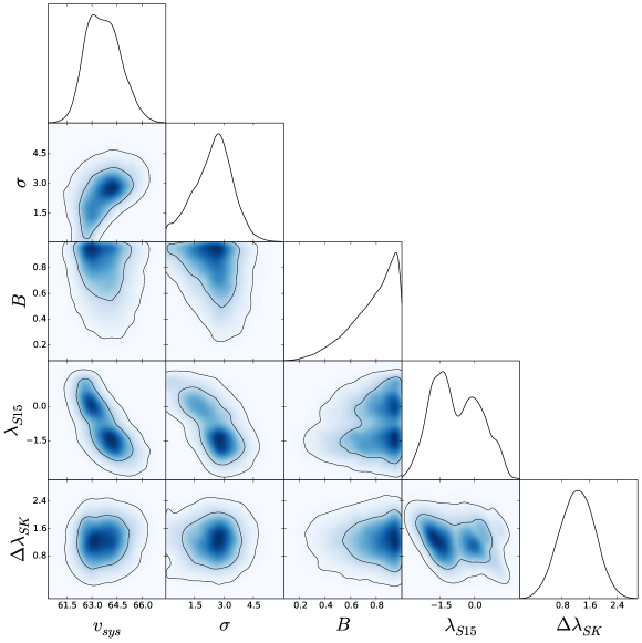
In Figure 2 we show the resulting posteriors for our fiducial model with mean period of 27 years. Although a large range of binary fractions is allowed ($B>0.2$), a high binary fraction is still preferred even for this relatively short mean period. The most probable velocity dispersion is 2.8${}_{-1.2}^{+0.7}$ km/s, where the uncertainties here denote the 68% credible interval. There is a small tail in the posterior extending to $\sigma=0$ km/s; note that this tail requires a binary fraction $B>0.8$, since binaries must make up all of the dispersion in this case. In addition, while there is a large uncertainty in either of the offsets $\lambda_{S15}$ and $\lambda_{K15}$, we find the relative offset $\Delta\lambda_{SK}$ is well constrained to be $1.2\pm 0.5$ km/s. The solution where both offsets are zero lies just outside the 95% probability contours. Hence, there seems to be a clear offset between the K15 and S15 datasets, but whether one or both of these datasets are offset with respect to the J16 measurements is quite uncertain given the small number of stars in the J16 sample.

The metallicity spread of Ret II is already strong evidence that Ret II is a galaxy rather than a globular cluster (Willman & Strader, 2012). Here we check whether its velocity dispersion paints a consistent picture of Ret II being a dark-matter dominated galaxy. If we assume the extreme scenario of no dark matter, we can estimate what the expected intrinsic dispersion of Ret II would be. Globular clusters of the Milky Way typically have mass-to-light ratios of 1-2 $M_{\odot}/L_{\odot}$. To be conservative, we choose the upper end of this range (2 $M_{\odot}/L_{\odot}$) and using Formula 2 in Wolf et al. (2010) we find this corresponds to $\sigma\approx 0.21$ km/s. Thus, we define the “no dark matter” scenario to be the regime $\sigma\leq 0.21$ km/s, where nearly all of Ret II’s dispersion would be due to binaries. For our fiducial 27-year mean period and a noninformative (log) prior in the dispersion, we thus infer a 1% probability for $M_{\odot}/L_{\odot}<2$; assuming a 180-year mean period (as in solar neighborhood binaries), the probability drops to 0.4%. In this regime where Ret II’s dispersion is due to binaries, the posteriors show there must be a positive offset of 1-3 km/s between the K15 velocities and the J16 velocities; in this case, the velocity changes due to binaries would be more dramatic, and hence requires a very high binary fraction. On the other hand, if the offsets are smaller (K15 $\lesssim$ 1 km/s, S15 $\lesssim$ 0 km/s) this does not rule out a high binary fraction, but it does rule out the zero-dispersion scenario.

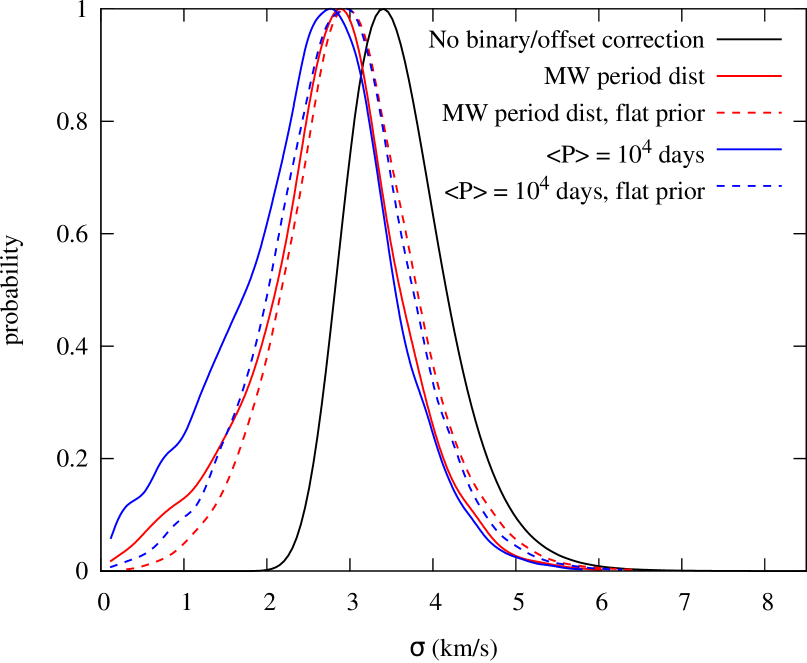
How sensitive are our results to the assumed binary population and priors? In Figure 3 we plot the inferred dispersion posterior using a few different models. First, we repeat the analysis but without including binaries or offsets (black line). In this case the most probable inferred dispersion is 3.5 km/s, and there is essentially zero probability of having an intrinsic dispersion less than 2 km/s. We plot our fiducial model with a mean period of 27 years (blue solid line), which used a log-prior in the dispersion; the same model with a uniform prior in the dispersion (blue dotted line) significantly reduces the probability of having a dispersion dominated by binaries, with essentially zero probability of $\sigma\approx 0$ km/s, while the most probable value is relatively unchanged. Finally, we try a model with a mean period of 180 years, similar to G-dwarfs in the Milky Way field, with a log-prior in dispersion (red solid line) as well as a uniform prior (red dashed line). Note that the most probable intrinsic dispersion is fairly robust to these changes in model or priors, in all cases being roughly 0.7 km/s lower compared to the uncorrected dispersion estimate. In addition, the tail going to very small intrinsic dispersions is only significant in our fiducial model (27-year mean period, log-prior in dispersion). With that said, it is certainly possible to increase the odds of having a binary-dominated dispersion if one assumes a shorter mean period; although it seems unlikely, this possibility cannot be ruled out entirely.

To check that the inferred offsets are consistent with a Gaussian velocity distribution plus binaries, we take the best-fit values for the offsets ($\lambda_{S15}=-1.48$, $\lambda_{K15}=-0.35$) and apply the correction to the the appropriate measurements in the data by subtracting these offsets. In Figure 4(a) we plot the cumulative distribution of $\Delta_{v}/\sigma_{2e}$, where $\Delta_{v}=|v_{1}-v_{2}|$ is the velocity difference between two consecutive epochs for each star and $\sigma_{2e}=\sqrt{e_{1}^{2}+e_{2}^{2}}$ is the corresponding uncertainty in this difference. For simplicity, we have only included the S15 and K15 datasets in this figure, for which the measurements are only 18 days apart, to minimize the effects of binaries. When the offset correction is not applied (red solid line), the cumulative distribution is systematically above what would be expected for a purely Gaussian distribution if the measurement errors properly reflect reality (although this is not statistically significant for any individual star except for the two that lie beyond 3$\sigma_{2e}$; the latter two have a high probability of being short-period binaries). However, when the measurements are adjusted for the best-fit offset values, the distribution follows a Gaussian quite closely (blue dashed line) with the exception of the two probable binary stars. Thus, the best-fit model does indeed appear consistent with a Gaussian velocity distribution plus a binary tail due to short period binaries. We should note that the effect of the offsets is not fully captured by the deviation of the red curve from Gaussianity here, because it does not indicate the sign of $v_{1}-v_{2}$; a random unaccounted-for measurement error could produce the same deviation. However, Figure 1(a) clearly indicates that most of the S15 measurements are systematically higher than the K15 measurements, so we can say with confidence that the correction applied here is reasonable.

Figure 3.— Posteriors in the intrinsic velocity dispersion, assuming different models and priors. The red and blue solid lines include binaries and offset parameters, assuming a log-prior in the velocity dispersion, whereas the corresponding dashed lines assume a uniform prior in the dispersion. Note that the most probable inferred dispersion is fairly robust, peaking around 2.8-2.9 km/s regardless of the binary population and dispersion priors chosen; this is roughly 0.7 km/s lower than the uncorrected estimate (black solid line).

(a) S15 and K15 only

(b) all datasets

Figure 4.— The fraction of stars with velocity changes greater than the combined measurement error $\sigma_{2e}$, where $\sigma_{2e}^{2}=\sigma_{1}^{2}+\sigma_{2}^{2}$ and $\sigma_{1}$ and $\sigma_{2}$ are the measurement errors in the first and second measurements respectively. In (a) we only include the S15 and K15 measurements, which are separated by only 18 days. Note that without correcting for offsets between datasets, the distribution (red solid curve) deviates from the expectation from Gaussian measurement error (solid black curve). However, when we apply a correction using our best-fit offset values (dashed blue), the distribution more closely follows the Gaussian limit, albeit with two outlier stars that are likely to be short-period binaries. In (b) we include all the measurements, again showing the data distribution (red dashed curve), along with the distribution of randomly resampled velocities assuming no binaries (dotted blue curve), and likewise assuming a mean period of 27 years and binary fraction of 0.5 (magenta curve).

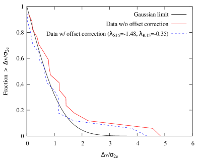
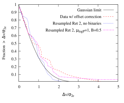
Next, we plot the distribution of $\Delta_{v}/\sigma_{2e}$ with all the measurements included in Figure 4(b). The red dashed curve corresponds to the data with the best-fit offset corrections applied; note that, compared to the short-timescale subset we plotted in Figure 4(a), there are significantly more measurements with velocity variations beyond the Gaussian expectation. Since these extra velocity changes occur over longer time scales ($\sim$ 1 year), they can be interpreted as being due to binary motion. This indicates that the two stars with large variations over 18 days between the S15 vs. K15 are not the sole driver behind the large binary fraction we have inferred. We verified this by repeating our analysis with those two stars removed from the sample, and found that a high binary fraction is nevertheless preferred by the data as a result of the significant velocity changes measured by the J16/R16 data. Finally, to verify that a galaxy with our best-fit parameters can reasonably reproduce the distribution of velocity variations we see in Ret II, we do random resamplings of the data and plot the resulting distributions. The blue dotted line shows a typical case with a binary fraction of zero; note that the large velocity changes in the tail are not well-reproduced, which is typically the case for many different random realizations. We then plot a typical case with a mean period of 27 years and a binary fraction of 0.5 (meaning half the stars in the sample are randomly assigned as binaries, and their binary properties are randomly sampled). It should be emphasized that due to the small sample size, the effect of binaries can vary considerably from realization to realization, depending on how many close binaries are present; in a few cases, there is no discernible binary tail at all. More typically, however, a tail exists and in many cases, as shown here, there may be one or two stars with velocity changes exceeding 5$\sigma_{2e}$, in some cases as large as 30-40 km/s. Such short-period binaries would be likely to have a velocity far from the galaxy’s systemic velocity at any given time, and hence would probably have been flagged as non-member stars. With that caveat aside, many realizations do show distributions that are broadly consistent with the data.

(a) $\sigma=0$ km/s

(b) $\sigma=2.7$ km/s

Figure 5.— Posteriors in velocity dispersion for simulated datasets where the velocity measurements are randomly resampled for each star in Ret II. In (a) we simulate a “galaxy” with intrinsic dispersion $\sigma$=0 km/s, while in (b) the simulated galaxy has intrinsic dispersion $\sigma$=2.7 km/s. Although each case has a high uncorrected dispersion $\sigma_{clip}$ determined from sigma-clipping, our method can clearly differentiate between these two scenarios despite the relatively small sample sizes.

5. Test of our method on simulated Ret II datasets

Our analysis shows that although Ret II appears to have a high binary fraction, its apparent velocity dispersion of $\sim$ 3 km/s is unlikely to be dominated by binary motion unless the measurements of K15 are systematically offset from those of J15 by $\approx$ 1-3 km/s. The latter possibility is disfavored by the data, but not beyond 95% confidence limits. This begs the question: if the close binary fraction does tend to be high in ultra-faint dSphs, given such small samples, can we be confident our method will distinguish between galaxies whose dispersion is strongly inflated by binary motion versus those that are not?

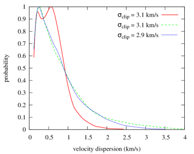
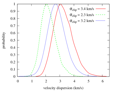
To investigate this question, we generate mock data by assuming a high binary fraction $B=0.9$ and short mean period of 27 years and resample all the velocities. We investigate two scenarios: in scenario 1, the intrinsic dispersion is $\sigma=0$ km/s (so any apparent velocity dispersion would be due entirely to binaries and measurement error); in scenario 2, we assume an intrinsic dispersion of $\sigma=2.7$ km/s, which is close to our best-fit dispersion of Ret II for the mean period assumed here. For each realization, we first calculate the uncorrected dispersion using 3$\sigma$-clipping: we find the maximum likelihood values of $\mu$, $\sigma$, then remove stars that lie beyond 3$\sigma$, and repeat as needed until no such outliers are present. In order to find cases that roughly resemble Ret II, we repeat many random realizations and keep three cases for which the uncorrected dispersion $\sigma_{clip}$ lies between 2.5-3.5 km/s. This required several realizations before three such cases were found for either scenario. In scenario 2 ($\sigma=2.7$ km/s), we did choose one realization with $\sigma_{clip}=2.3$ km/s to see if a nonzero intrinsic dispersion can be recovered even for a lower $\sigma_{clip}$ value. After applying our analysis to these mock data, the resulting posteriors in the intrinsic dispersion are plotted in Figure 5(a) for the scenario where $\sigma=0$ km/s. In all three cases we infer that $\sigma<1.5$ km/s at greater than 90% confidence; the most probable intrinsic dispersion is well below 1 km/s in all cases. Thus, our method appears unlikely to find a peak at $\sigma>2$ km/s if the apparent velocity dispersion is dominated by binaries. In 5(b) we plot the resulting posteriors for the cases where the true $\sigma=2.7$ km/s. Here we see that $\sigma=0$ km/s is ruled out in all cases; in none of these cases do we find a most probable intrinsic dispersion lower than 2 km/s. This builds confidence that, despite the relatively small sample size, our binary-corrected velocity dispersions can be trusted.

As we mentioned above, despite Ret II having a most probable intrinsic dispersion of 3 km/s in our analysis, there is still a nonzero probability of $\sigma=0$ km/s. What are we to make of this? First keep in mind that if the K15 are measurements are not systematically offset from the higher-resolution J15 measurements by $\approx$ 1-3 km/s, the probability of Ret II having $\sigma=0$ km/s essentially vanishes. If we retain the possibility of a large offset between the K15 and J15 datasets, then there are three possible explanations: either (i) Ret II’s true intrinsic dispersion is in fact somewhere between 0-3 km/s, and the peak appearing at 3 km/s is merely due to the small sample size; (ii) Ret II has a close binary fraction even higher than what we have assumed in the above mock data, and hence show velocity variations beyond what the realizations above could produce; or (iii) there is some additional systematic in the velocity measurements that is producing velocity changes that appear consistent with short-period binary motion. Additional spectroscopic measurements will be necessary, to distinguish between these scenarios with a high degree of confidence. Nevertheless, our mock data runs bolster confidence that Ret II’s apparent dispersion is unlikely to be entirely dominated by binary orbital motion.

6. Discussion

The result that Ret II’s dispersion is unlikely to be entirely due to binaries is not surprising, given that its very low metallicities and metallicity spread clearly identify it as a dwarf galaxy rather than a globular cluster. However, the clear preference for a high binary fraction and/or short mean period in Ret II is consistent with a similar result found for the Segue 1 dSph (Martinez et al., 2011). If this pattern of a high close binary fraction holds up in other ultra-faints, it would be strong evidence that the close binary fraction of a star population is a strong function of metallicity, with low metallicity populations harboring a greater fraction of close binaries. This anticorrelation between close binary fraction and metallicity has already been pointed out in Milky Way field binaries (Moe et al., 2018; El-Badry & Rix, 2018; Badenes et al., 2018). Whether this is due to a high binary fraction, a short mean period, or some combination of the two remains to be determined; as discussed in Minor (2013), the degeneracy between binary fraction and the period distribution cannot be broken purely by radial velocity measurements without a very large sample with measurements at several epochs. Unfortunately such a large sample is unattainable at present for individual ultra-faint dwarfs.

The most promising approach for breaking the degeneracy between binary fraction and period distribution would be to combine radial velocity measurements with CMD fitting; the latter approach is demonstrated in Geha et al. (2013) and is sensitive only to the binary fraction and stellar masses, not to the periods. An additional independent handle on the binary fraction is possible if main sequence stars are included in the sample, for which binary spectral fitting is possible (El-Badry et al., 2018a, b). As we have hinted in Section 2, our method for generating the binary and non-binary likelihoods can be recast in the form of a hierarchical Bayesian model: for individual stars, their orbital parameters (e.g. $v_{cm},P,q$) are marginalized over, while the prior distributions in these parameters are constrained for the whole population at the next level of inference. This approach, which has been used elsewhere to constrain the distribution of orbital parameters in binaries and exoplanets (Price-Whelan et al., 2018; Foreman-Mackey et al., 2014; Hogg et al., 2010), can be incorporated naturally into the methodology used here; in principle, it allows for color-magnitude information and radial velocities to be fit under the same hierarchical framework, and could be applied to a combination of dSph datasets over many epochs to find detailed binary constraints. The demonstration of this more generalized approach in the context of dwarf galaxies is left to future work.

The decrease of the velocity dispersion due to the binary correction has implications for the implied dark matter halo of Ret II. The half-light mass ($M_{1/2}$) of a dispersion supported system is well measured at the half-light radius and it is proportional to $\sigma^{2}$ (Walker et al., 2009; Wolf et al., 2010). The binary corrected half-light mass will decrease by a factor $\sigma^{2}$. Assuming $\sigma=3.3$ (Simon et al., 2015) we find that the half-mass decreases by a factor of 0.72, decreasing to $M_{1/2}=4.0\times 10^{5}M_{\odot}$ (from $M_{1/2}=5.6\times 10^{5}M_{\odot}$). Searches for dark matter annihilation in ultra-faint dwarfs require an accurate determination of the J-Factor, an integral over the dark matter density squared. The J-Factor is proportional to $\sigma^{4}$ (Pace & Strigari, 2018) and for Ret II the J-Factor will decrease by a factor 0.52. Using the J-Factor value from Pace & Strigari (2018), we find the binary corrected J-Factor to be $\log_{10}{\left(J/{\rm GeV^{2}\,cm^{-5}}\right)}=18.58$ (from 18.87).

7. Conclusion

We have applied a Bayesian method to model multi-epoch radial velocities in the ultra-faint dwarf Reticulum II, fully accounting for the effects of binary orbital motion and systematic offsets between different spectroscopic datasets. Our primary results are encapsulated in Figures 2 and 3, where we infer the intrinsic dispersion and binary fraction of Ret II. Despite the relatively small sample size (26 stars in total), we find that the binary fraction of Ret II is higher than 0.5 at the 90% confidence level, if the mean orbital period is assumed to be 30 years or longer. Despite this high binary fraction, the best-fit intrinsic dispersion of Ret II is 2.8${}_{-1.2}^{+0.7}$ km/s, consistent with Ret II having a large mass-to-light ratio. Our best-fit velocity dispersion is smaller than previous estimates and implies a weaker dark matter annihilation signal, with the J-factor reduced by a factor of $\approx$ 0.5 compared to the results of Simon et al. (2015). Assuming a mean period of $10^{4}$ days (which was recently inferred in low-metallicity Milky Way binaries in Moe et al. 2018), we estimate a $\approx$ 1% probability that Ret II’s dispersion is due to binaries rather than dark matter, corresponding to the regime $M_{\odot}/{L_{\odot}}\approx$ 2. These results are thus consistent with Ret II being a dark matter-dominated galaxy to high significance, in agreement with the expectation from its large metallicity dispersion.

Beyond the importance of obtaining unbiased mass estimates of ultra-faint dwarfs, binary populations in these objects are interesting in their own right as they may hold clues to star formation in extremely metal-poor environments. The fact that Ret II appears to have a high close binary fraction is consistent with previous results from the Segue 1 ultra-faint dwarf, and echoes similar results from Milky Way halo stars that suggest that metal-poor star populations have a relatively high fraction of close binaries. A more robust and detailed characterization of binary populations in dwarf galaxies will require a larger multi-epoch sample for a large number of dwarfs, a combination of deep photometry and high-resolution spectroscopy, and the application of a fully hierarchical version of the Bayesian method we have applied in this paper. Over the long term, the binary populations in these extreme objects might hold vital clues to a deeper understanding of the physics underlying star formation.

References

- Ackermann et al. (2015) Ackermann, M. et al. 2015, Physical Review Letters, 115, 231301
- Badenes et al. (2018) Badenes, C. et al. 2018, ApJ, 854, 147
- Bechtol et al. (2015) Bechtol, K. et al. 2015, ApJ, 807, 50
- Brown et al. (2012) Brown, T. M. et al. 2012, ApJ, 753, L21
- Carney et al. (2005) Carney, B. W., Aguilar, L. A., Latham, D. W., & Laird, J. B. 2005, AJ, 129, 1886
- Drlica-Wagner et al. (2015) Drlica-Wagner, A. et al. 2015, ApJ, 809, L4
- Duquennoy & Mayor (1991) Duquennoy, A. & Mayor, M. 1991, A&A, 248, 485
- El-Badry & Rix (2018) El-Badry, K. & Rix, H.-W. 2018, ArXiv e-prints
- El-Badry et al. (2018a) El-Badry, K., Rix, H.-W., Ting, Y.-S., Weisz, D. R., Bergemann, M., Cargile, P., Conroy, C., & Eilers, A.-C. 2018a, MNRAS, 473, 5043
- El-Badry et al. (2018b) El-Badry, K. et al. 2018b, MNRAS, 476, 528
- Elbert et al. (2018) Elbert, O. D., Bullock, J. S., Kaplinghat, M., Garrison-Kimmel, S., Graus, A. S., & Rocha, M. 2018, ApJ, 853, 109
- Foreman-Mackey et al. (2014) Foreman-Mackey, D., Hogg, D. W., & Morton, T. D. 2014, ApJ, 795, 64
- Geha et al. (2013) Geha, M. et al. 2013, ApJ, 771, 29
- Hogg et al. (2010) Hogg, D. W., Myers, A. D., & Bovy, J. 2010, ApJ, 725, 2166
- Ji et al. (2016a) Ji, A. P., Frebel, A., Simon, J. D., & Chiti, A. 2016a, ApJ, 830, 93
- Ji et al. (2016b) Ji, A. P., Frebel, A., Simon, J. D., & Geha, M. 2016b, ApJ, 817, 41
- Kim & Jerjen (2015) Kim, D. & Jerjen, H. 2015, ApJ, 808, L39
- Kirby et al. (2015) Kirby, E. N., Cohen, J. G., Simon, J. D., & Guhathakurta, P. 2015, ApJ, 814, L7
- Kirby et al. (2017) Kirby, E. N., Cohen, J. G., Simon, J. D., Guhathakurta, P., Thygesen, A. O., & Duggan, G. E. 2017, ApJ, 838, 83
- Kirby et al. (2008) Kirby, E. N., Simon, J. D., Geha, M., Guhathakurta, P., & Frebel, A. 2008, ApJ, 685, L43
- Koch et al. (2009) Koch, A., Wilkinson, M. I., Kleyna, J. T., Irwin, M., Zucker, D. B., Belokurov, V., Gilmore, G. F., Fellhauer, M., & Evans, N. W. 2009, ApJ, 690, 453
- Koposov et al. (2015a) Koposov, S. E., Belokurov, V., Torrealba, G., & Evans, N. W. 2015a, ApJ, 805, 130
- Koposov et al. (2015b) Koposov, S. E. et al. 2015b, ApJ, 811, 62
- Latham et al. (2002) Latham, D. W., Stefanik, R. P., Torres, G., Davis, R. J., Mazeh, T., Carney, B. W., Laird, J. B., & Morse, J. A. 2002, AJ, 124, 1144
- Li et al. (2018) Li, T. S. et al. 2018, ApJ, 857, 145
- Lovell et al. (2014) Lovell, M. R., Frenk, C. S., Eke, V. R., Jenkins, A., Gao, L., & Theuns, T. 2014, MNRAS, 439, 300
- Luque et al. (2016) Luque, E. et al. 2016, MNRAS, 458, 603
- Luque et al. (2017a) —. 2017a, ArXiv e-prints
- Luque et al. (2017b) —. 2017b, MNRAS, 468, 97
- Martin et al. (2016) Martin, N. F. et al. 2016, ApJ, 818, 40
- Martinez et al. (2011) Martinez, G. D., Minor, Q. E., Bullock, J., Kaplinghat, M., Simon, J. D., & Geha, M. 2011, ApJ, 738, 55
- McConnachie & Côté (2010) McConnachie, A. W. & Côté, P. 2010, ApJ, 722, L209
- Minor (2013) Minor, Q. E. 2013, ApJ, 779, 116
- Minor et al. (2010) Minor, Q. E., Martinez, G., Bullock, J., Kaplinghat, M., & Trainor, R. 2010, ApJ, 721, 1142
- Moe et al. (2018) Moe, M., Kratter, K. M., & Badenes, C. 2018, ArXiv e-prints
- Olszewski et al. (1996) Olszewski, E. W., Pryor, C., & Armandroff, T. E. 1996, AJ, 111, 750
- Pace & Strigari (2018) Pace, A. B. & Strigari, L. E. 2018, ArXiv e-prints
- Price-Whelan et al. (2018) Price-Whelan, A. M. et al. 2018, AJ, 156, 18
- Raghavan et al. (2010) Raghavan, D. et al. 2010, ApJS, 190, 1
- Rocha et al. (2013) Rocha, M., Peter, A. H. G., Bullock, J. S., Kaplinghat, M., Garrison-Kimmel, S., Oñorbe, J., & Moustakas, L. A. 2013, MNRAS, 430, 81
- Roederer et al. (2016) Roederer, I. U. et al. 2016, AJ, 151, 82
- Simon & Geha (2007) Simon, J. D. & Geha, M. 2007, ApJ, 670, 313
- Simon et al. (2011) Simon, J. D. et al. 2011, ApJ, 733, 46
- Simon et al. (2015) —. 2015, ApJ, 808, 95
- Spencer et al. (2017) Spencer, M. E., Mateo, M., Walker, M. G., Olszewski, E. W., McConnachie, A. W., Kirby, E. N., & Koch, A. 2017, AJ, 153, 254
- Walker et al. (2009) Walker, M. G., Mateo, M., Olszewski, E. W., Peñarrubia, J., Wyn Evans, N., & Gilmore, G. 2009, ApJ, 704, 1274
- Wilkinson et al. (2002) Wilkinson, M. I., Kleyna, J., Evans, N. W., & Gilmore, G. 2002, MNRAS, 330, 778
- Willman & Strader (2012) Willman, B. & Strader, J. 2012, AJ, 144, 76
- Wolf et al. (2010) Wolf, J., Martinez, G. D., Bullock, J. S., Kaplinghat, M., Geha, M., Muñoz, R. R., Simon, J. D., & Avedo, F. F. 2010, MNRAS, 406, 1220