Testing dynamical vacuum models with CMB power spectrum from Planck
Abstract
The cosmic expansion is computed for various dynamical vacuum models and confronted to the Cosmic Microwave Background (CMB) power spectrum from Planck. We also combined CMB in a joint analysis with other probes to place constraints on the cosmological parameters of the dynamical vacuum models. We find that all models are very efficient and in very good agreement with the data. Considering that the interaction term of the dark sector is given in terms of matter and radiation densities we find that the corresponding model shows a small but non-zero deviation from cosmology, nevertheless the confidence level is close to .
Keywords: cosmology: cosmic background radiation, cosmological parameters, dark matter, dark energy
1 Introduction
The comprehensive analysis of a large family of observational data indicate that around of the Universe content corresponds to unknown sectors, usually called dark matter (around ) and dark energy (around ). Dynamically, the latter component plays a key role in cosmic expansion because it is responsible for the outstanding phenomenon of cosmic acceleration (Perlmutter et al. 1998; Riess et al. 1998; Astier et al. 2007; Komatsu et al. 2011; Suzuki et al. 2012; Ade et al. 2016; Aghanim et al. 2018). It is worth mentioning that the nature of dark energy (hereafter DE) has been a topic of interest ever since its first appearance in Einstein’s equations as a cosmological constant. Even though the term was briefly discarded as unnecessary, the cosmological constant is to date the most favored candidate as a dark energy which coexists with cold dark matter (CDM) and ordinary baryonic matter (see Peebles & Ratra 2003, for review). These components form the so called CDM model which fits accurately the current cosmological data.
Although the CDM model is considered as a successful cosmic scenario, it is not without its problems (Weinberg 1989; Padmanabhan 2003; Perivolaropoulos 2008; Padilla 2015). Examples of theoretical impairments of the model include the fine tuning and coincidence problems. The fine tuning problem reflects the gap between the expected (Planck natural unit) vacuum energy density , which, using quantum field theory (QFT), is calculated at a remarkable orders of magnitude larger that the observed value of at the present time. On the other hand, the coincidence problem sources from the approximate equality of and prior to the present time, even though the former is a dynamical quantity and the latter is a constant.
These problems have given rise to a large body of cosmological models which mainly extends the traditional Einstein-Hilbert action of general relativity using either a new field (Horndeski 1974; Brans & Dicke 1961; Nicolis, Rattazzi & Trincherini 2009; Urena - Lopez 2016), or a modified gravity theory that increases the number of degrees of freedom (Buchdahl 1970; Bengochea & Ferraro 2009; Sotiriou & Faraoni 2010; Clifton, Ferreira, Padilla & Skordis 2012; Nunes et. al. 2016; Nunes, Pan & Saridakis 2016, see also Copeland, Sami & Tsujikawa 2006; Caldwell & Kamionkowski 2009; Amendola & Tsujikawa 2010). Among the class of DE models, the introduction of a dynamical vacuum, , is perhaps the simplest modification of the Einstein-Hilbert action towards alleviating the aforementioned theoretical issues (see Basilakos 2009; Basilakos, Lima & Sola 2013; Perico, Lima, Basilakos & Sola 2013; Basilakos, Mavromatos & Sola 2016). Here, the time dependence is not introduced via the equation of state (EoS) parameter which, like the CDM, is strictly set to , but is inherited to the pressure through . Notice, that the idea to deal with a vacuum which varies with cosmic time (or redshift) has a long history in cosmology and it is perfectly allowed by the cosmological principle (Ozer & Taha 1986; Bertolami 1986; Chen & Wu 1990; Carvalho, Lima & Waga 1992; Lima & Maia 1993; Salim & Waga 1993; Arcuri & Waga 1994; Lima & Carvalho 1994; Lima & Trodden 1996; John & Joseph 2000; Lima, Maia & Pires 2000; Novello, Barcelos-Neto & Salim 2001; Vishwakarma 2001; Cunha, Lima & Pires 2002; Schutzhold 2002a, 2002b; Aldrovandi, Beltran Almeida & Pereira 2005; Carneiro & Lima 2005; Pan 2018).
Usually, the dynamical vacuum energy density evolves slowly as a power series of the Hubble rate (for a review see Shapiro & Sola 2002; Grande et. al. 2011; Sola 2013, 2014; Gomez, Sola & Basilakos 2015). In this scenario, the decaying vacuum energy density has an interesting feature, namely it predicts that the spacetime emerges from a non-singular initial de Sitter vacuum stage, hence the phase of the universe changes in a smooth way from inflation to a radiation epoch (”graceful exit”). Then the universe enters into the dark-matter and vacuum-dominated phases, before finally, entering to a late-time de Sitter phase (Basilakos et. al. 2013, 2016; Perico et. al. 2013). From the observational view point, recently (Sola, Gomez - Valent & de Cruz Perez 2017a, 2017b, 2018) tested the performance of the running vacuum models against the latest cosmological data and they found that the models are favored over the usual CDM model at statistical level (see also Zhao et al. 2017). These results have led to growing interest in cosmological models.
In this work we attempt to study the performance of various dynamical vacuum models at the expansion level. Specifically, a likelihood analysis, involving the Planck CMB power spectrum (Ade et. al. 2016), is implemented in order to constrain the models. Up to now, for these models only the set of the CMB shift parameters have been used in order to test the dynamical vacuum scenarios close to recombination. Then we combine CMB in an overall likelihood analysis with other cosmological probes (SNe type Ia, BAOs, ) in order to extract the probability distribution (via Monte Carlo MCMC method) of the solutions for a large set of cosmological parameters, as well as, to search for deviations from the concordance CDM model for which .
The structure of our paper is as follows: in section 2 we provide a brief introduction of the running vacuum cosmology and we present the most popular models that have appeared in the literature. In section 3 we discuss the methodology and the cosmological data that we utilize and we perform a detailed statistical analysis aiming to provide the corresponding best fit values and contour plots for the current models. Finally, we discuss our results in the conclusions.
2 Background expansion in running vacuum models
In this section we briefly describe the main features of the dynamical vacuum models for which is not constant but evolves with cosmic time. This is perfectly allowed by the cosmological principle embedded in the FLRW metric (Perico et. al. 2013). In general, if we model the expanding universe as a mixture of perfect fluids then the total energy momentum tensor is given by
| (1) |
where is the 4-velocity field. In this case the components of are written as
| (2) |
where the quantities and are the total pressure and energy density in the comoving frame , respectively. The next step is to apply the covariant local conservation law for the mixture, namely . Inserting Eq.(1) into the latter expression and with the aid of the relation (which comes from the fact that for any four-velocity vector, we have ) we arrive at (Grande, Pelinson & Sola 2009):
| (3) |
For a Friedmann-Lemaître-Robertson-Walker (FLRW) metric, it is easy to check that for a comoving frame (), one obtains:
| (4) |
and thus Eq.(3) reduces to
| (5) |
where is the Hubble parameter and is the scale factor of the universe normalized to unity at the present epoch. For the rest of the paper we focus on the spatially flat FLRW metric.
In the aforementioned discussion we did not address the physics of the fluids involved. The total density receives contributions from non-relativistic matter (cold dark matter and baryons) (), radiation () and vacuum (). In this context the index specifies the specific components of the cosmic fluid, namely . Assuming that baryons and radiation are self-conserved, namely the corresponding densities evolve in the nominal way and the overall conservation law (5) becomes
| (6) |
or
| (7) |
| (8) |
Notice that is the interaction term between dark matter and running vacuum, such that a small amount of vacuum decays into dark matter or vice versa. It is worth mentioning that the above expression is the outcome of imposing the covariant conservation of the total energy density of the combined system of matter and vacuum, hence is a direct consequence of the Bianchi identity in the context of general relativity. Of course in the case of the concordance CDM model (=const., ), we recover the standard dark matter conservation law .
Within this framework, the Friedmann equations of the system formed by the above fluid components are given by (see Sola et. al. 2017a, and references therein):
| (9) |
| (10) |
2.1 Specific models
Now let us briefly present the running vacuum models studied in this article. For each one of these models we provide the term of interaction and thus we calculate the evolution of main cosmological quantities, namely , and . Notice that the baryon and the radiation densities obey the standard laws, namely and respectively. Specifically, the current models read as follows.
The first model under consideration is the running vacuum model as described in (Basilakos 2009; Basilakos et. al. 2013, 2016; Perico et. al. 2013) (hereafter CDM1). In this case we have , hence solving the system of equations (7)-(8) one finds an expression for the evolution of both densities:
| (11) |
| (12) |
while the normalized Hubble parameter is given by
| (13) |
The second phenomenological model that we take into account is that with (hereafter CDM2). In this context, we have
| (14) |
| (15) |
and
| (16) |
The final vacuum model consists of (hereafter CDM3). Within this framework the basic cosmological quantities become
| (17) |
| (18) |
| (19) |
It is important to note that for the aforementioned equations boil down to those of CDM, as they should.
3 Fitting running vacuum models to the Planck CMB spectrum
For this analysis, the publicly available CAMB code was modified to admit dynamical vacuum models, and used in combination with the MCMC package to restrain the usual set of cosmological parameters of the standard model for Cosmology, with the addition of the dynamical vacuum parameter . We use the Planck satellite, 2015 release which includes the CMB power spectrum, TT, TE, EE + lowP (Ade et. al., 2016). For completeness we also give the constrains of the CDM model. Notice that the parameter space is , where is the mass variance at Mpc, , spectral index, is the optical depth. Notice that in CAMB, the density of photons is calculated through , with being the Stefan - Boltzmann constant, and the temperature of the CMB.
| Model | CDM | CDM1 | CDM2 | CDM3 |
|---|---|---|---|---|
| - | ||||
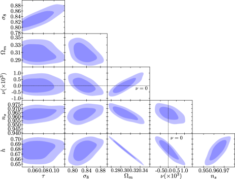
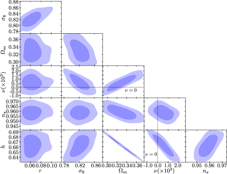
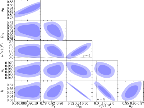
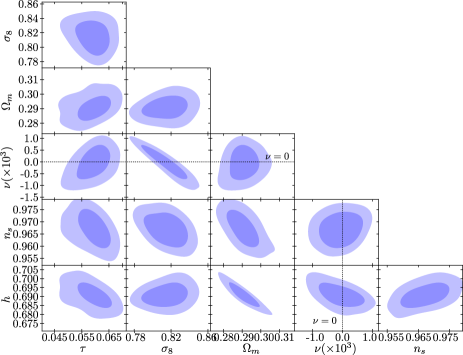
In Table I we show an overall presentation of the current observational constraints imposed by the CMB spectrum, while in Figs. 1, 2 and 3 we plot the and contours in various planes for the explored CDM models.
In particular, we find:
-
•
For the CDM1 model we find , , , , and .
-
•
In the case of CDM2 model we obtain , , , , and .
-
•
For the CDM3 model: , , , , and .
-
•
In order to check the differences of the CDMi models from the concordance CDM case for which . Specifically, we find , , , and .
where we have quoted error bars.
We observe that the results from CAMB suggest that the best fit parameters of the dynamical vacuum models are in agreement with those of CDM case. Moreover, the current observational constraints are compatible with those of TT, TE, EE + lowE Planck 2018 data provided by Aghanim et. al. (2018) (see also Ade et. al. 2016), namely , , , and . Concerning the Hubble constant problem, namely the observed Hubble constant Km/s/Mpc found by Riess et. al. (2018), is in tension with that of Planck Km/s/Mpc (Aghanim et. al. 2018), we find that the values extracted from the models are closer to the latter case (see also Sola et. al. 2017b). Moreover our results are in agreement with those of Shanks, Hogarth & Metcalfe (2018), who found Km/s/Mpc using the GAIA parallax distances of Milky Way Cepheids. However, the reader has to keep in mind that other studies support larger values of (cf. Lima & Cunha2014; Beaton et al. 2016; Freedman 2017).
Moreover, we would also like to compare our results with those of Yang et al. (2018), who have tested three scalar field DE models against various datasets. Particularly, for the Planck data the constraints of Yang et al. (2018), [see Tables 1,2,4] stand as follows. For the potential they found , , , , and . In the case of they obtained , , , , and . Lastly, for the potential , where is the Planck mass, Yang et al. (2018), found , , , , and . Obviously the constraints of the models (see Table I) are compatible within with those of scalar field DE models.
3.1 Combining with other probes
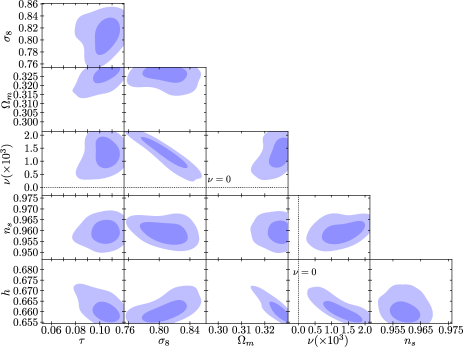
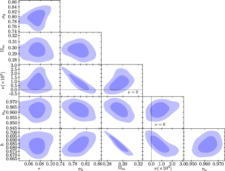
In this section we implement a joint likelihood analysis using SNIa from JLA sample (Betoule et. al. 2014), Baryonic Acoustic Oscillations (BAOs) (Blake et. al. 2011; Alam et. al. 2016) and measurements of Riess et. al. 2018, in order to place tight constraints on the corresponding parameter space of the models. The best fit parameters are listed in Table II. In order to visualize the solution space in Figs.4, 5 and 6 we show the 1 and 2 contours for various planes. Specifically, the joint likelihood function peaks at (with the corresponding 68% errors)
-
•
For the CDM1 model: , , , , and .
-
•
For the CDM2 model: , , , , , and .
-
•
For the CDM3 model: , , , , , and .
-
•
Lastly, for the usual CDM we find , , , and .
We find that the incorporation of more data sets via joint analyses improves the fitting for all models, hence the current running vacuum models are very efficient and in very good agreement with observations. Among the three models the CDM1 is the one with a small but non-zero deviation from the concordance CDM cosmology. Indeed we find that the deviation parameter is different from zero at level.
First we verified that the combined constraints of the models (see Table II) are in agreement within errors with those of Yang et al. (2018), who considered the case of scalar field DE (see also Park & Ratra 2018), where these authors found: , , , , and [model ], , , , , and [model ] and finally , , , , and for the potential .
Concerning the CDM1 model our results can be compared with those of Wang (2018), who combined SNIa/H(z)/BAO/CMB data. Notice that regarding the cosmological parameters our CMBshift/SNIa/BAO/ constraints are similar (within ) with those of Sola et al. (2018) (see also Gomez et. al. 2015, Sola et. al. 2017a, 2017b, and references therein) who found, combing cosmic chronometer, SNIa (JLA), CMB shift parameters and BAO data, =, =, and = for the CDM1, CDM2 and CDM3 models, respectively. Regarding the CDM2,3 models our constraints are in agreement with those of von Marttens et al. (2018) who used CMB (via CLASS code) in a joint analysis with , SNIa, cosmic chronometer and BAO data.
Although our observational constraints are in qualitative agreement with previous studies (cf. Gomez et. al. 2015, Sola et. al. 2017a, 2017b, 2018) we would like to spell out clearly the main reason why the results of the present work are novel. Indeed, to our knowledge, our analysis includes the Planck CMB power spectrum (via CAMB) in a large family of dynamical vacuum models and thus we can trace the Hubble expansion of the models in the recombination era.
| Model | CDM | CDM1 | CDM2 | CDM3 |
|---|---|---|---|---|
| - | ||||
4 Conclusions
We extracted observational constraints on various dynamical vacuum models, using the CMB power spectrum from Planck. We used the most popular models and in all of them we studied their deviation from the usual CDM model through a sole parameter. Modifying CAMB we found that the best fit parameters of the explored running vacuum models are in agreement with those of CDM. For completeness we combined the CMB spectrum in a joint analysis with other cosmological probes (SNe type Ia, BAOs, ) in order to place tight constraints on the cosmological parameters of the dynamical vacuum models. We find that CDM2 and CDM3 do not show deviations from the CDM case. However, for the CDM1 vacuum model,we found a small but non-zero deviation from CDM, where the confidence level is close to . This is an indication that dark energy could be dynamical.
Acknowledgements
Spyros Basilakos would like to acknowledge
support by the Research Center for Astronomy of the Academy
of Athens in the context of the program “Tracing the Cosmic
Acceleration”.
References
- [Ade et al. 2016] Ade, P. A. R., et al. 2016, A&A, 594A, 1P (Plank data)
- [1] Aghanim, N. et al., 2018 [Planck Collaboration], [arXiv:1807.06209 [astro-ph.CO]]
- [2] Alam, S., et al. 2017, [BOSS Collaboration], Mon. Not. Roy. Astron. Soc. 470, no. 3, 2617 [arXiv:1607.03155 [astro-ph.CO]].
- [3] Aldrovandi, R., Beltran Almeida, J. P., & Pereira, J.G. 2005, Grav. Cosmol. 11, 277
- [4] Amendola, L., & Tsujikawa, S., 2010, Dark Energy Theory and Observations, Cambridge University Press, Cambridge UK
- [5] Arcuri, R. C., & Waga, I. 1994, Phys. Rev. D 50, 2928
- [6] Astier, P. et al., 2007, Astrophys. J. 659, 98
- [7] Basilakos, S. 2009, Astron. & Astrophys., 508, 575
- [8] Basilakos, S., Lima, J., & Sola, J. 2013 Int.J.Mod.Phys. D22 1342008
- [9] Basilakos, S., Mavromatos, N., & Sola, J., 2016, Universe, 2 14
- [10] Beaton R. L., et al., 2016, ApJ, 832, 210
- [11] Bengochea, G.R., & Ferraro, R., 2009, Phys. Rev. D 79, 124019
- [12] Bertolami, O., 1986, Nuovo Cimento 93, 36
- [13] Betoule, M., Kessler, R., Guy, J., Mosher, J., Hardin, D. et al., 2014, Astron. & Astrophys., A22, 568
- [14] Blake, C. et al., 2011, Mon. Not. Roy. Astron. Soc. 418, 1707 [arXiv:1108.2635 [astro-ph.CO]]
- [15] Brans, C., & Dicke, R. H., 1961, Phys. Rev. 124, 195
- [16] Buchdahl, H. A., 1970, Mon. Not. Roy. astron. Soc. 150, 1
- [17] Caldwell, R. R., & Kamionkowski, M., 2009, Ann.Rev.Nucl.Part.Sci., 59, 397, arXiv:0903.0866
- [18] Carneiro, S., Lima, J. A. S., 2005, Int. J. Mod. Phys. A 20, 2465
- [19] Carvalho, J. C., Lima, J. A. S., & Waga, I., 1992, Phys. Rev. D 46, 2404
- [20] Chen, W., & Wu, Y. S., 1990, Phys. Rev. D 41, 695
- [21] Clifton, T., Ferreira, P. G., Padilla, A., & Skordis, C., 2012, Phys. Rep. 513, 1
- [22] Copeland, E. J., Sami, M., & Tsujikawa, S., 2006, Intern. Journal of Modern Physics D, 15, 1753
- [23] Cunha, J. V., Lima, J.A. S., & Pires, N., 2002, Astron. and Astrophys.390,809
- [24] W. L. Freedam, Nature Astronomy, 2017, 1, 0169
- [25] A. Gomez-Valent, J. Sola and S. Basilakos, 2015, JCAP 01, 004
- [26] Grande, J., Pelinson, A., & Sola, J., 2009, Phys. Rev. D 79, 043006, arXiv:0809.3462.
- [27] Grande, J., Sola, J., Basilakos, S., & Plionis, M., 2011, JCAP, 08, 007
- [28] Horndeski, G.W., 1974, Int. J. Theor. Phys. 10, 363
- [29] John, M. V.,& Joseph, K. B., 2000, Phys. Rev. D 61, 087304
- [30] Komatsu, E., et al., 2011, Astrophys. J. Suppl. 192, 18
- [31] Lima, J. A. S., & Maia, J. M. F., 1993, Mod. Phys. Lett. A 08, 591
- [32] Lima, J. A. S., & Carvalho, J. C., 1994, Gen. Rel. Grav. 26,909
- [33] Lima, J. A. S., & Trodden, M., 1996, Phys. Rev. D 53, 4280
- [34] Lima, J. A. S., Maia, J. M. F., & N. Pires, N., 2000, IAU Symposium 198, 111
- [35] Lima, J.A.S., & Cunha J. V., 2014, ApJL, 781, L38
- [36] Nicolis, A., Rattazzi, R., & Trincherini, E., 2009 Phys. Rev. D 79, 064036
- [37] Novello, M., Barcelos-Neto, J., & Salim, J. M., 2001, Class. Quant. Grav. 18, 1261
- [38] Nunes, R. C., Pan, S., & Saridakis, E.N., 2016, JCAP 1608, 011
- [39] Nunes, R. C., Bonilla, A., Pan, S., & Saridakis, E. N., 2016, EPJC77, 230
- [40] Ozer, M., & Taha, O., 1987, Phys. Lett. A 171, 363 (1986) Nucl. Phys. B 287, 776
- [41] Padilla, A., 2015, arXiv:1502.05296
- [42] Padmanabhan, T., 2003, Phys. Rept. 380, 235
- [43] Pan, S., 2018, MPLA 33, 1850003
- [44] Park, C. G., & Ratra, B., 2018, arXiv:1807.07421
- [45] Peebles, P. J., & Ratra, B., 2003, Rev. Mod. Phys. 75, 559
- [46] Perico, E.L.D., Lima, J.A.S., Basilakos, S., & Sola, J., 2013, Phys. Rev. D 88, 063531
- [47] Perivolaropoulos, L., 2008, arXiv:0811.4684
- [48] Perlmutter, S., et al., 1998, Astrophys. J. 517, 565
- [49] Riess, A. G., et al., 1998, Astron J. 116, 1009
- [50] Riess, A. G., et al., 2018, Astrophys. J. 855, 18
- [51] Salim, J., & Waga, I., 1993, Class. Quant. Grav. 10, 1767
- [52] Schutzhold, R., 2002, Phys. Rev. Lett. 89, 081302
- [53] Schutzhold, R., 2002, Int. J. Mod. Phys. A 17, 4359
- [54] Shanks, T., Hogarth, L., & Metcalfe, N., 2018, [arXiv:1810.02595]
- [55] Shapiro, I. L., & Sola, J., 2002, Phys. Lett. B 530, 10
- [56] Sola, J., 2013, Cosmological constant and vacuum energy: old and new ideas , J. Phys. Conf. Ser. 453, 012015 [e-Print: arXiv:1306.1527]
- [57] Sola, J., 2014 ’Vacuum energy and cosmological evolution’ , AIP Conf.Proc. 1606 19 [e-Print: arXiv:1402.7049];
- [58] Sola, J., Gomez-Valent, A., & de Cruz Pérez, J., 2017 Astrophys.J. 836, 43
- [59] Sola, J., Gomez-Valent, A., & de Cruz Pérez, J., 2017 Physics Letters B, 774, 317
- [60] Sola, J., de Cruz Pérez, J., & Gomez-Valent, A., 2018 Mon. Not. R. Astron. Soc., 478, 4357
- [61] Sotiriou, T. P., & Faraoni, V., 2010, Rev. Mod. Phys. 82, 451
- [62] Suzuki, N., et al., 2012, Astrophys. J. 746, 85
- [63] Urena - Lopez, L.A., 2016, J. Phys. Conf Ser. 761, 012076
- [64] Vishwakarma, R. G., 2001, Class. Quant. Grav. 18, 1159
- [Wang 2018] Wang, D., 2018, arXiv:1801.02371
- [65] Weinberg, S., 1989, Rev. Mod. Phys. 61, 1
- [66] von Marttens, R., Casarini L., Mota D. F., Zimdahl W., 2019, Phys. Dark Un., 23, 100248
- [67] Yang, W., Shahalam, M., Pal, B., Pan, S., & Wang, A., 2018 arXiv:1810.08586 [gr-qc].
- [68] Zhao, G.B., et al., 2017, Nat. Astron. 1, 627