The initial mass function in the Coma Berenices dwarf galaxy from deep near-infrared HST observations.

Abstract

We use deep $HST$ WFC3/IR imaging to study the Initial Mass Function (IMF) of the ultra faint dwarf galaxy Coma Berenices (Com Ber). Our observations reach the lowest stellar mass ever probed in a resolved galaxy, with 50% completeness at $\sim 0.17$ M_⊙. Unresolved background galaxies however limit our purity below $\sim 0.23$ M_⊙. If modeled with a single power law, we find that the IMF slope is $-1.45^{+0.29}_{-0.3}$ (68% credible intervals), compared to a Milky Way value of $-2.3$. For a broken power law, we obtain a low-mass slope of $-1.18_{-0.33}^{+0.49}$, a high-mass slope of $-1.88_{-0.49}^{+0.43}$ and a break mass of $0.57_{-0.08}^{+0.12}$ M_⊙, compared to $-1.3$, $-2.3$ and 0.5 M_⊙ for a Kroupa IMF. For a log-normal IMF model we obtain values of $0.33_{-0.16}^{+0.15}$ M_⊙ for the location parameter and of $0.68_{-0.12}^{+0.17}$ for $\sigma$ (0.22 M_⊙ and 0.57 for the Chabrier system IMF). All three parametrizations produce similar agreement with the data. Our results agree with previous analysis of shallower optical HST data. However analysis of similar optical data of other dwarfs finds IMFs significantly more bottom-light than in the Milky Way. These results suggest two, non mutually exclusive, possibilities: that the discrepancy of the dwarf galaxies IMF with respect to the Milky Way is, at least partly, an artifact of using a single power law model, and that there is real variance in the IMF at low masses between the currently studied nearby dwarfs, with Com Ber being similar to the Milky Way, but other dwarfs differing significantly.

1 Introduction

In recent years the question of the universality of the initial mass function (IMF) across different environments as well as throughout cosmic history has seen the rise of a new interest, thanks to several new results. van Dokkum & Conroy (2010, 2011, 2012) and Conroy & van Dokkum (2012) have used integrated spectra of giant elliptical galaxies to claim that these environments show a more bottom heavy IMF with respect to the Galaxy (see also Spiniello et al., 2012). Cappellari et al. (2012) claim a similar bottom-heaviness for the IMF of early type galaxies using a different approach based on the comparison between masses derived by dynamical models (constrained by integral-field spectroscopy) and masses derived from stellar population synthesis (constrained by photometric measurements). More recently, these results have been questioned by Smith (2014) who compare the spectroscopic and dynamical methods. While the global trends from the two approaches are similar, such detailed comparison shows large systematics and lack of agreement for the objects that can be studied using both approaches, thus questioning the reliability of the individual results. Furthermore, Newman et al. (2017) compare dynamical, spectroscopic, and, in addition, lensing-based IMF estimates for a sample of three nearby giant ellipticals. Their results are that when the underlying IMF is parametrized as a single or broken power law, the results for the three methods disagree for 2 out of the 3 galaxies in the sample. However, using more flexible, including non-parameteric, IMF forms partly relieves this tension. It must be noted however that the mismatch pointed out by Smith (2014) might be due to the existence of radial gradients in the IMF of giant ellipticals (Martín-Navarro et al., 2015; Lyubenova et al., 2016; van Dokkum et al., 2017). Thus the differences in individual galaxies results can be related to the use of different apertures between the different sets of observations.

While studies of integrated light from external galaxies allow us to probe a large range of environments, studies based on resolved star counts can help reaching a finer level of detail, less dependent on modeling assumptions. On the other end, the majority of resolved studies of the IMF at low stellar masses have been limited to the nearby Galactic field and star clusters, which do not reflect the wide range of environments over which the IMF is routinely applied.

For the Milky Way field, Salpeter (1955) originally proposed a single power-law IMF, but modern observations show a break in the IMF slope at low masses (for a review, see Bastian et al., 2010). The IMF is parameterized as either a log-normal distribution with a turn-over mass near 0.25M_⊙ (Chabrier, 2003; Bochanski et al., 2010), or a broken power law, $\mathrm{d}N/\mathrm{d}m\propto m^{\alpha}$, with slope ${\alpha}=−2.3$ above 0.5 M_⊙, and shallower slope of ${\alpha}=-1.3$ below (Kroupa, 2002). The stellar mass at which this slope transition occurs is predicted to depend on the physical properties of the stellar birth cloud (Larson, 2005).

Milky Way open clusters provide a relatively large stellar mass range over which to measure the IMF (0.08 to 100, the upper limit depending on the cluster’s age M_⊙, see e.g. Moraux et al., 2003; Da Rio et al., 2012; Hußmann et al., 2012; Weisz et al., 2013; Andersen et al., 2017), but are predominantly metal-rich and only the youngest are not affected by mass segregation and evaporation. HST studies of Galactic globular clusters probe the IMF down to main sequence masses between 0.1 and 0.8 M_⊙ (Paust et al., 2010; Leigh et al., 2012; Sollima & Baumgardt, 2017; Webb et al., 2017), and find slope values covering a wide range from -1.5 to +0.2, thus encompassing the mean value estimated in the Galactic field. However, dynamical evolution, such as mass segregation and evaporation, preferentially affects low-mass stars and can significantly change the slope of the mass function in these concentrated systems (Vesperini & Heggie, 1997). Dwarf galaxies provide a similarly low metallicity environment, but have relaxation times many times the age of the Universe, therefore minimizing any corrections for dynamical evolution (see Section 6.1 of Gennaro et al., 2018).

Several recent studies exist that try to address the question of the IMF universality (or lack thereof) in nearby dwarf Milky Way satellite galaxies. Given their different properties (e.g., morphology, metallicity, star formation history), these dwarf satellites are interesting targets to explore possible IMF differences with respect to the Milky Way.

One of the first of such studies is the one by Wyse et al. (2002), who measured an IMF slope of $-1.8$ for the Ursa Minor dwarf spheroidal in the 0.4 – 0.7 M_⊙ range, using $HST$ WFPC2 data. Recently Kalirai et al. (2013), used $HST$ ACS/WFC to reach $\sim$0.4 M_⊙ in the Small Magellanic Cloud outskirts. They found that the IMF there has a slope of $\sim-1.9$, shallower than the typical Salpeter value of $-2.35$. Geha et al. (2013) also used ACS/WFC to study the IMF of the Hercules and Leo IV ultra-faint dwarf galaxies (UFDs), measuring slopes of $-1.2$ and $-1.3$ respectively. Gennaro et al. (2018) extended the analysis of Geha et al. (2013) adding 4 more UFDs to the sample, namely Boötes I (Boo I), Canes Venatici II (CVn II), Coma Berenices (Com Ber) and Ursa Major I (UMa I). They found similar results to Geha et al. (2013) for Hercules and Leo IV, and, when using a single power law model, they found an overall shallower slope for the UFDs IMF when compared to the Salpeter value. El-Badry et al. (2017) note that a flatter than Salpeter slope could be a natural result if the true, underlying IMF is in fact a log-normal. A single power law fit to masses drawn from a Chabrier (2003) IMF, limited to a mass range of 0.4-0.8 M_⊙ (the one accessible in the Kalirai et al., 2013; Geha et al., 2013; Gennaro et al., 2018, studies), gives in fact a slope $\alpha=-1.55$.

Within their sample, Gennaro et al. (2018) noted that for the 2 closest UFDs, Boo I and Com Ber, a Salpeter value could be ruled out only at 1$\sigma$ level, while for the other UFDs the discrepancy was larger, up to more than 3$\sigma$ for Hercules and Leo IV. Moreover, when modeling the IMF with a log-normal function, the results for the overall sample were more consistent with the Milky Way values (Chabrier, 2003; Bochanski et al., 2010), with again Boo I and Com Ber showing the least dissimilarity with respect to the Galaxy.

The typical limiting mass of the Gennaro et al. (2018) ACS data was 0.4 – 0.5 M_⊙. In the current work we present a study of the IMF of Com Ber, the closest of the 6 UFDs in the ACS sample, using deeper infrared data. ComBer is a very faint system, with $M_{V}\sim-3.8$ mag. Its mean metallicity is [Fe/H] $=-2.6$ dex, with a spread of about 1 dex (Brown et al., 2014). From optical data its distance has been determined to be $\sim 43$ kpc (Brown et al., 2014). Its half-light radius is 77 pc, which at its distance subtends an angle of 6.15 arcminutes.

We have targeted Com Ber as part of an $HST$ program (GO:13449, PI: M. Geha) which used the infrared channel of the WFC3 camera, better suited for efficient observations of faint, cool stars. Using WFC3, our observations reached down to $\sim 0.2$M_⊙ in Com Ber, thus allowing the deepest extra-Galactic study of the IMF so far. Com Ber shows neither kinematic nor photometric evidence for tidal disruption (Simon & Geha, 2007; Muñoz et al., 2010). While its proximity to the Milky Way makes it vulnerable to tides, these processes should not bias the IMF, since Com Ber 2-body relaxation time is of the order of $5\times 10^{3}$ Gyr (see equation (5) of Gennaro et al., 2018), and thus it is not expected to suffer from mass-dependent losses. Of the nearest UFDs, Com Ber has the highest surface brightness ($\mu_{V}$ = 27.3 mag arcsec⁻²), and thus is a very suitable candidate for a deep IMF study.

2 The data

The data used in this paper were obtained as part of the HST GO program 13449 (PI: M. Geha). A total of 44 WFC3/IR orbits were allocated to this program, with an equal number of ACS/WFC parallel images; the latter target the outskirts of Com Ber. This work only deals with the WFC3/IR images, covering the center of Com Ber.

2.1 Observing strategy

We utilized the WFC3/IR instrument in the F110W and F160W filters. We imaged the galaxy in a 2x2 tiles mosaic, and reduced and analyzed the 4 tiles independently of each other. The program consisted of 44 HST orbits, equally divided among the 4 tiles. The 11 orbits per tile were split with 4 orbits in F110W and 7 in F160W. Each orbit was split in 2 exposures, thus resulting in 8 dithered exposures in F110W and 14 dithered exposures in F160W per tile. The resulting exposure times are 10994 seconds in F110W and 18989 seconds in F160W per tile.

2.2 Data reduction

WFC3/IR images in filters that are sensitive to the Earth’s atmosphere Hei 1.083 $\mu$m line afterglow can suffer from a time-variable background. This is due to the change in the depth of the atmosphere along the line of sight and is especially severe at ingress/egress of $HST$ from occultation during its orbit around the Earth. This problem may affect F110W observations, and thus impact the up-the-ramp fitting performed by the calwfc3 pipeline, which assumes a constant background, thus producing images with artificially increased noise. To reduce the problem, the individual up-the-ramp non-destructive reads of a WFC3/IR Multiaccum exposure can be equalized by subtracting the average sky value measured from the difference between two consecutive reads. We used software developed by a former WFC3 team member (B. Hilbert, priv. comm.) to treat the images before running the standard calwfc3 reduction process (see also Brammer, 2016, for a summary on the He I related problem and a very similar mitigation strategy, as well as publicly available software performing similar pre-processing of WFC3/IR images).

The images were aligned and drizzled using the standard Drizzlepac tools (Gonzaga et al., 2012), using the F110W band as the astrometric reference. Images were drizzled to rotation=0 (North up), a scale of 60 mas/pix, and pixfrac of 0.8. The latter controls the fraction by which the input pixels are “shrunk” before being drizzled onto the output image grid, i.e. the drizzle ”drop” size. The final drizzled images were converted to counts images in preparation for use with the stand-alone DAOPHOT-II package (Stetson, 1987).

2.3 Photometry

Figure 1: Left: Color-magnitude diagram showing sources identified as point sources (blue) and as extended ones (red), with superimposed a density plot of the Hubble Ultra deep field objects (grey scale, see text for more details). Right: m₁₆₀ luminosity function for the same objects. The dashed blue line at m₁₆₀ = 28.6 mag indicates where our background objects counts depart from the HUDF counts; this is where we set our limiting depth for further analysis. In the right panel the HUDFs counts have been normalized to the area of our mosaic.

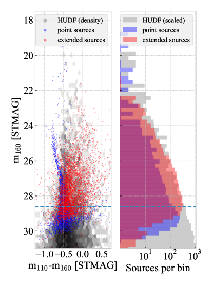
PSF fitting photometry was conducted using the stand-alone DAOPHOT-II package, to obtain F110W and F160W magnitudes calibrated in the STMAG system. Thresholds in the $\chi$ and sharpness values are used to distinguish point sources from resolved background objects. The combined color-magnitude diagram (CMD) for the 4 tiles is shown in Figure 1.

To test our ability to resolve background sources, we compare the luminosity function of resolved objects, i.e. all the photometric detections that do not make the $\chi$ and sharpness cut, to that of the Hubble Ultra deep Field (HUDF), using the catalog made available by Rafelski et al. (2015). Because there is no F110W observation for the HUDF, we mock F110W data by linearly interpolating the fluxes in the F105W and F125W.

Figure 1 shows the HUFD sources, scaled to the total area of our observations. The luminosity function of our extended, background sources matches that in the HUDF very well down to about F160W = 28.6 mag, below which our extended background source luminosity function falls below the HUFD one. This means that we fail to characterize background objects as extended sources beyond this point. Even though our 50% completeness limit for point sources is about 0.8 mag fainter than 28.6 mag in F160W (see Section 2.4), we choose to preserve the purity of our catalog by limiting our analysis to stars brighter than F160W = 28.6 mag, where we can safely rely on our $\chi$-sharpness selection. This magnitude value corresponds to about 0.23 M_⊙ at the distance and extinction of Com Ber. The mass at the 50% completeness limit, F160W $\sim$ 29.4 mag, is instead about 0.17 M_⊙, thus the loss in mass range corresponding to the adopted conservative cut in magnitude is small but not negligible. The half-mass radius for a typical dwarf galaxy, 300 pc, is unresolved in WFC3/IR beyond $\sim 1$ Gpc, corresponding to a distance modulus of 40 mag and to a redshift, $z\sim 0.15$. Dwarf galaxies of intrinsic brightness $M_{160}\sim-10$ mag at such a distance contribute to the unresolved background sources seen in Figure 1, with brighter dwarfs galaxies contributing up to even larger distances. This problem will be alleviated (by a factor of 3 at fixed wavelength) when the James Webb Space Telescope will become operational.

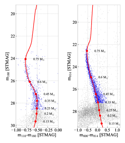
We further select our data by excluding the sources on the red giant branch (RGB). In practice, we adopt a bright magnitude cut at F160W = 23 mag. This cut allows us to ignore the RGB region, where the stellar models tend to not be able to reproduce the observed colors, in our simulations versus data comparison. Given the faster evolution on the RGB relative to the main sequence, this bright limit has no significant impact on the mass range probed. The final number of selected stars per tile is 223, 163, 149, and 182 respectively, for a total of 717.

The selected data are highlighted in a CMD in Fig. 2, where the IR data presented in this paper are also compared to the optical Com Ber data first presented by Brown et al. (2014), and used for deriving the IMF in Gennaro et al. (2018). The figure shows how the new data reach a lower stellar mass, thus giving more mass leverage for the IMF determination with respect to the existing optical data. The optical observations cover however a larger area on the sky, and thus the number of Com Ber members is larger in the optical than in the IR CMD.

Figure 2: Left: IR data used in this paper. Right: optical data from Brown et al. (2014), used for deriving the IMF in Gennaro et al. (2018). The grey points indicate all the objects identified as point sources. The blue points represent the data used for inferring the IMF in either this work or Gennaro et al. (2018). In red is a 14.0 Gyr, [Fe/H] = -2.6 dex isochrone from VandenBerg et al. (2014), transformed into the appropriate passbands using the MARCS model atmospheres (Gustafsson et al., 2008). For the IR isochrone we apply the corrrection described in Section 3. The red points mark several mass values along the isochrone. The y-axes in the two panels have the same total magnitude range and are arranged vertically to get the same y-position for the 0.45 M_⊙ model.

2.4 Artificial star tests

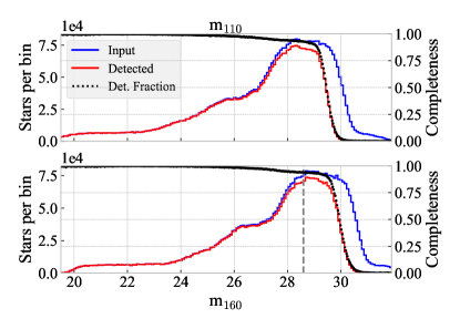
We perform artificial star tests to obtain an estimate of the noise distribution of our sources. We use these experiments in our synthetic color-magnitude diagram simulation when fitting for the IMF parameters. The artificial star tests were produced by randomly populating isochrones at [Fe/H]=$-1.6$, $-2.0$, and $-2.4$ dex and age = 10, 11, 12, and 13 Gyr. Each pass of artificial star tests inserted 1000 stars into the images and blindly recovered them, comparing output to input. Specifically, each pass drew 800 stars from the isochrones, with significant scattering (to fill in the CMD parameter space), plus another 200 stars at random locations over the entire CMD (to avoid having gaps in the artificial star CMD coverage). The result places the most weight where we need it (i.e., near real isochrones, where most stars should fall) but characterizes the uncertainties and incompleteness over a broad swath of CMD space. The same $\chi$ and sharpness criteria applied to the real stars are applied to the artificial stars, and if the latter do not pass the $\chi$-sharpness test, they are considered undetected.

Figure 3 shows the luminosity functions of the inserted stars (input magnitudes in each band) and the luminosity function of the detected ones (again input magnitudes), as well as the ratio of the two. The vertical dashed line in the $m_{160}$ bottom panel corresponds to 28.6 magnitudes, i.e., the limit at which we loose the ability to detect extended background sources in our data. This is the faint cut we have to impose to our catalog, in order to avoid contamination from unresolved background galaxies. It is clear that our ability to detect point sources extends well past this limit, with the 50% completeness level being about 29.4 magnitudes in F160W. However we choose to keep the highest possible purity in our catalog, at the cost of loosing some depth.

Figure 3: Luminosity distributions of the input magnitudes of the artificial stars (blue), and the same but only for stars that have a valid output magnitude (red); all 4 tiles are shown together. Superimposed, black dotted line, on a different y-axis is the ratio between the 2, i.e. the completeness fraction as function of the input magnitude of the artificial stars. The vertical dashed line at 28.6 magnitudes, in the $m_{160}$ panel (bottom), shows the adopted magnitude limit for which extended sources can still be robustly identified, and which is well above the 50% completeness limit.

2.5 Residual Photometric Uncertainty

During the analysis stage we observed that the photometric uncertainty encoded in the artificial stars was slightly underestimated. In particular, the scatter of simulated color magnitude diagrams, built using the artificial star tests and realistic metallicity and age distributions for ComBer, showed a narrower main sequence than that observed. This extra error may be due to the limitations of the PSF model constructed from the undersampled data. An other possibility is a metallicity effect. While we are using the most up-to-date metallicity distribution function (MDF) available for Com Ber (Brown et al., 2014), if the true intrinsic distribution is slightly broader, it may produce extra CMD width, with respect to what we can reproduce using our adopted MDF.

We determined that an extra error term of 0.0175 mag (standard deviation) in each photometric band was enough to force the simulations to agree with the data, in terms of simulated main sequence width. This extra error is implemented in our subsequent analysis by further scattering each artificial star output magnitude using a draw from a normal distribution with width equal to 0.0175 mag. It is worth noting that this error term is quite small, on the order of the photometric repeatability quoted by the WFC3/IR instrument team ($\sim$0.5-1%, see the WFC3 data handbook), and thus our heuristic approach of adding an extra random Gaussian term is appropriate and sufficient for our purposes.

3 The models

We adopt the same $\alpha$-enhanced stellar models as in Brown et al. (2014) computed using the Victoria-Regina evolutionary code (see VandenBerg et al., 2014, and references therein), in the metallicity range $-4.0<$ [Fe/H] $<-1.0$ dex. These models have [$\alpha$/Fe] = +0.4 dex, and a further oxygen enhancement, $\Delta$[O/Fe], that increases at decreasing [Fe/H] values (details in Section 3.2 of Brown et al., 2014). We transform the models into the observational plane using tables of synthetic fluxes computed with the MARCS code (Gustafsson et al., 2008), and the most up-to-date WFC3 filter throughputs. The Brown et al. (2014) oxygen-enhanced models were computed ad-hoc and extend only down to 0.4 M_⊙. In order to further extend the grid of models to lower masses, we computed $\alpha$-enhanced models without extra $\Delta$[O/Fe]. These models are then ”patched” by forcing them to agree with the oxygen-enhanced ones at 0.4 M_⊙, and by assuming that a rigid translation applies to the model for all masses below 0.4 M_⊙.

Figure 4: Calibration of the isocrone library with respect to the M92 ridge line (top panels) and the Com Ber ridge line (bottom panels). The density plots on the left column are on a logarithmic scale.

3.1 First empirical correction: M92 ridge line

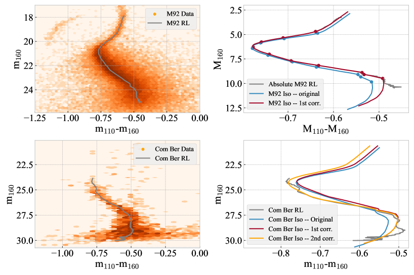
Brown et al. (2014) showed a very good agreement of the stellar models with the M92 cluster ridge line in the HST/ACS optical (F606W-F814W, F814W) color-magnitude diagram. M92 is the most metal-poor cluster for which we have good WFC3/IR data from the HST Galactic Bulge Treasury Program (GO: 11664, PI: T. M. Brown). Such data can be used for calibration of the stellar models in the F110W and F160W bands. We do not observe the same agreement of the models with the M92 IR data. However, rather than fine-tuning the isochrone parameters to try and obtain a better fit of the M92 ridge line, we assume that the cluster parameters for which the models give good agreement in the optical are valid: $(m-M)_{0}=14.62$ mag, E(B-V)= 0.023 mag, age = 13.2 Gyr, [Fe/H] = -2.3 dex. We derive an empirical calibration of the IR models with respect to the M92 ridge line in the following steps:

1. we generate a ridge line for the M92 (F110W,F160W) data, using the technique described in Correnti et al. (2016), this step is shown in Figure 4, top right

2. we subtract the extinction in each band and distance modulus from the M92 ridge line using $(m-M)_{0}=14.62$ mag, E(B-V)= 0.023 mag, $R_{V}$=3.1 and assuming that the extinction law can be described by a Cardelli et al. (1989) model. This results in $(A_{110},A_{160})=(0.0228,0.0144)$ mag at the respective effective wavelengths of each of the F110W and F160W filters. The distance and extinction subtracted ridge line is shown as ”Absolute M92 RL” in the top-right panel of Fig. 4

3. We compute the isocrone for the nominal M92 values of age (13.2 Gyr), [Fe/H] (-2.3 dex) and [$\alpha$/Fe] (0.4 dex), with [O/Fe] = +0.64 dex. This is shown as ”original” in Figure 4, top right

4. we identify ”characteristic points” on both the M92 ridge line and the original isochrone. These are visible features in the 2 curves, and we assume that, for a calibrated model, their color and magnitudes need to match exactly. These characteristic points are marked by dots in the top right panel of Fig. 4 (the dots for the corrected model lie, by definition, on the ridge line). Some of these points are identifiable with significant evolutionary stages (i.e., the main sequence turn-off, the low-mass main sequence kink, the base of the red giant branch). Others have been chosen based on morphological characteristics of the isochrones (e.g the mid-point in the sub-giant branch, slight bends along the main sequence between the kink and turn-off)

5. we compute the differences in F160W magnitude and F110W-F160W color between the points corresponding to the same stages along two curves

6. we interpolate such correction as function of $\log g$ in the model

7. assume that the same correction in $\log g$ applies for all ages and metallicities

3.2 Second empirical correction: Com Ber ridge line

The above sequence of steps does not yet provide a complete agreement when the models for the peak of the Com Ber metallicity distribution function are computed and overplotted on the data.

We thus define a second calibration step, this time in apparent magnitude space. The steps are the following:

1. build a ridge line for the Com Ber population. This is shown in the bottom left panel of Figure 4

2. compute the isochrone for the bulk of the Com Ber population, corresponding to the peak of the metallicity distribution of the galaxy, [Fe/H] $=-2.6$ dex and at an age of 14.0 Gyr, and at its distance, (m-M)₀= 17.956 mag, and extinction, $A_{\mathrm{V}}=0.124$ (all values from Brown et al., 2014). From $A_{\mathrm{V}}$ we derive $(A_{110},A_{160})=(0.0398,0.0251)$ mag. This is the isochrone labeled as ”original” in the lower-right panel of Fig. 4

3. apply the empirical calibration described in Sect. 3.1 to the original isochrone thus obtaining the isochrone labeled as ”1st corr.” in the lower-right panel of Fig. 4

4. compute residual color offsets between the ”1st corr.” isochrone and the Com Ber Ridge Line

5. interpolate the residual offset as function of m₁₆₀

The combination of the two calibration steps gives us models that agree very well with the Com Ber ridge line. The residual offsets visible in the lower right panel of Figure 4, between the final model (orange) and the ridge line(gray) are of the order of $\lesssim 0.01$ mag.

It must be noted that the extent of the discrepancy between the uncorrected models and the M92 or Com Ber ridge lines is of the order of 0.05 mag maximum, and only in the coolest regions of the CMD. This is probably related to uncertainties in the model atmospheres of cool stars in the near-IR. Around 0.3 M_⊙, where the most serious discrepancies arise, the mass-luminosity relation in our passbands is of about 0.1 M_⊙/mag, thus an error of 0.05 mag in color, would correspond to only 5 thousandths M_⊙. The impact of such errors on the IMF determination is negligible.

4 The method

Our analysis aims at deriving the best parameters for an underlying model describing the IMF of Com Ber. We assume three possible IMF parametrizations: a single power law (SPL), a broken power law (BPL), and a log-normal function (LN). The models functional forms are thus specified:

The mass distributions are specified as

$$p_{\mathrm{SPL}}(m|\alpha)\propto \;m^{\alpha}$$ (1)

$$p_{\mathrm{BPL}}(m|\alpha_{1},\alpha_{2},m_{brk})\propto \;m^{\alpha_{1}},m>m_{brk}$$ (2a)

$$\;km^{\alpha_{2}},m<m_{brk}$$ (2b)

$$\;k=m_{brk}^{\alpha_{1}-\alpha_{2}}$$

$$p_{\mathrm{LN}}(m|m_{c},\sigma)\propto \;\frac{1}{m}e^{-\frac{1}{2}\left(\frac{\log m-\log(m_{c})}{\sigma}\right)^{2}}$$ (3)

The method we use to fit for the IMF parameters is presented in Gennaro et al. (2018) and it is based on a combination of Approximate Bayesian Computation (ABC) techniques, Kernel Distance methods and Markov Chain Monte Carlo sampling. The statistical model used to describe the observed CMD is defined in the framework of Poisson Point Processes (see Gennaro et al., 2015, and references therein).

In brief, the method consists of i) moving in the parameter space by drawing sets of parameters, using existing Markov Chain Monte Carlo methods (we adopt the Foreman-Mackey et al., 2013 implementation of the Goodman & Weare, 2010 affine-invariant sampler). As an example, for the single power-law model, the parameters set would consist of a total number of stars, a slope, and a binary fraction, ii) building a synthetic CMD based on those parameters, and using the stellar models described in Sect. 3 and the artificial stars experiments described in Sect. 2.4, iii) comparing the simulated and observed data sets by defining a suitable distance between them. The distance measurement is based on kernel distance methods (see Gennaro et al., 2018, for more details), iv) define a maximum acceptable distance threshold, retaining parameter sets for which the distance is below the threshold. The fact that the threshold is small, but not zero, makes this method an Approximate, and not an exact Bayesian Computation.

The ensemble of accepted parameter sets is an approximation of their posterior probability density function. Each parameter set specification includes the specification of the total intensity, i.e., the integral of the IMF in the mass interval under consideration. The boundaries of the integral, in our case are $[0.175,8]\mathrm{~{}M}_{\odot}$. The intensity can be regarded as a normalization factor. The total number of generated stars is a drawn from a Poisson distribution with mean equal to the total intensity.

Similarly to Gennaro et al. (2018) we specify the IMF in terms of the system mass. For single stars, this is equivalent to the stellar mass. In the case of binaries, the system mass is equal to the sum of the primary and secondary mass. We assume that the binary mass ratio (i.e., the ratio of the secondary to the primary mass) is uniformly distributed between 0 and 1. While the mass ratio distribution is fixed, the binary fraction is a parameter of our IMF models.

In building the synthetic CMDs that are compared to the observed ones, we adopt the star formation history and metallicity distribution function derived for Com Ber in Brown et al. (2014). We also adopt their distance modulus and E(B-V) reddening. The latter is converted into F110W and F160W extinction values using the Cardelli et al. (1989) extinction law (see Section 3.2 for the numerical values of these parameters).

Table 1: Best-fit parameters and credible intervals for the 3 IMF models. The credible intervals are defined as containing $(0.6827,0.9545,0.9973)$ of the posterior.

Model	Parameter	Average	68% Cr.I.	95% Cr.I.	99% Cr.I.
Single Power law	Slope	$-1.45$	$[-1.75,-1.16]$	$[-2.11,-0.88]$	$[-2.56,-0.68]$
	Binary Fraction	0.25	$[0.0,0.33]$	$[0.0,0.58]$	$[0.0,0.83]$
Broken Power law	Low-mass Slope	$-1.18$	$[-1.51,-0.69]$	$[-1.93,-0.49]$	$[-1.97,-0.11]$
	High-mass Slope	$-1.88$	$[-2.37,-1.45]$	$[-2.66,-1.00]$	$[-2.95,-1.00]$
	Break mass	0.56	$[0.44,0.68]$	$[0.36,0.79]$	$[0.30,0.80]$
	Binary Fraction	0.23	$[0.07,0.35]$	$[0.00,0.50]$	$[0.00,0.86]$
Log-normal	$m_{c}$	0.33	$[0.16,0.49]$	$[0.03,0.65]$	$[0.02,0.86]$
	$\sigma$	0.68	$[0.56,0.84]$	$[0.35,0.95]$	$[0.23,0.99]$
	Binary Fraction	0.20	$[0.0,0.26]$	$[0.0,0.53]$	$[0.0,0.96]$

5 Results

Given that both the photometry and the artificial star tests have been performed on each of the 4 tiles separately, we perform MCMC experiments on the individual tiles, and then combine the posteriors to obtain the average properties of the Com Ber IMF across the tiles. As in Paper I, the MCMC experiments are performed assuming a flat prior on the intensity, i.e. the total number of expected stars. This easily allows choosing a different prior, by using a reweighting of the samples. Specifically, for our final results we adopt a uniform prior on the logarithm of the intensity, which is achieved by reweighting individual samples by intensity^-1. This prior choice is well justified: it is an observed fact, as well as a prediction of cosmological models, that the Universe contains more small galaxies than large ones. For example, in the Schechter (1976) galaxy luminosity function, at least well below the cutoff luminosity $L^{*}$, the dependency of the number of galaxies with their luminosity (of which the number of stars within a galaxy is a proxy) is that of a power-law with index close to $-1$. Therefore, a priori, smaller galaxies, containing a lower number of stars, are preferred.

The results for the 4-tile-combined posteriors of the IMF parameters, for the three different model choices (Single Power Law, Broken Power Law, Log-normal; hereafter SPL, BPL and LN, respectively) are displayed in Figure 5, while the best-fit values and credible intervals are summarized in Table 1. We use the mean of the marginal posterior of each parameter as the best-fit estimator. Our credible intervals are defined as the smallest intervals containing the 68%, 95% and 99% of the marginal probability, we sometimes refer to these as 1$\sigma$, 2$\sigma$ and 3$\sigma$ intervals respectively.

Figure 6 shows a comparison between synthetic CMDs and luminosity functions computed for the best fit parameter sets and the data. The right panels of this Figure show the difference between the complete set of extracted masses (the IMF, orange) and the masses of the objects that are “observed” in the synthetic CMD (the present day mass function, PDMF).

Figure 5: Corner plots of the posterior distributions of IMF parameters for the 3 different models. The vertical dashed lines indicate the 16, 50 (median), 84 percentiles of the marginal distributions.

6 Discussion

Figure 6: Comparison between the simulations (blue) for the best-fit parameters of each model and the data (red). Left: simulated and observed luminosity function in the F160W band. Center: simulated and observed CMD. Right: draws from the underlying IMF (yellow/orange), and corresponding Present Day Mass Function (PDMF, teal), i.e., the mass distribution of the stellar systems that are actually observed in the simulated CMD. The dashed lines show the ratio of the two, i.e., the completeness as function of system mass; to obtain the dashed line a much higher number of stars have been drawn than those shown here. Note that the PDMF extends beyond the turnoff mass because there are binary systems of total mass larger than the turnoff mass, where only the secondary star, less massive than such limit, survives.

6.1 Comparison between the different models

From Figure 6 we can see that the three IMF models give very similar results. The $m_{160}$ luminosity functions for the best fit parameters for each of the three models (left columns in the figure) do trace the observed luminosity function, even if with some differences in the details. From the right panels of the Figure 6, the best-fit parameters for the three IMF models produce very similar PDMFs (green), regardless of the different underlying IMFs (orange). We note some discrepancy between the models, especially at the high-mass end, where there are the fewest stars. Another fact emerges quite clearly: no obvious turnover of the IMF is observed. The SPL model gives as good a fit to the data down to our limiting mass as the BPL and LN ones; if anything the best-fit SPL model seems to be the one producing the luminosity function giving the best qualitative agreement at faint magnitudes.

To provide a more quantitative assessment of the goodness of fit (gof) and see whether any of the 3 models is inconsistent, in a gof sense, with the data, we devised an ad-hoc strategy. Our fitting method uses an ABC approach, and thus bypasses an explicit calculation of the likelihood. Methods like Bayes Factors, Akaike- or Bayesian Information criteria (AIC, BIC) cannot therefore be used here. Our acceptance of a proposed parameter set, $\vec{\theta_{i}}$ relies on generating a CMD using $\vec{\theta_{i}}$, which we call $y_{i}$ and determine whether $y_{i}$ is close to the observed CMD, $y_{obs}$. The distance between the simulated and observed CMD is given by equation (10) of Gennaro et al. (2018); we will call such distance $\rho(y_{i},y_{obs})$.

Our gof criterion is a modification of the gof statistic based on the posterior predictive distribution proposed by Lemaire et al. (2016), and it consists of:

• take two subsets of draws from the posterior, a training set $\{\vec{\theta_{j}}\}_{j\in J}$, and a test set $\{\vec{\theta_{k}}\}_{k\in K}$ possibly from two disjoint parts of the MCMC chain. In practice we use the first 250 draws for $J$ and the last 1000 for $K$

• compute, for each $k\in K$, the average distance of the corresponding CMD, $\vec{\theta_{k}}$ to the $\{\vec{\theta_{j}}\}_{j\in J}$:

  $$D_{post,k}=\frac{1}{n_{J}}\sum_{j\in J}\rho(y_{k},y_{j}),$$ (2)

  where $n_{J}$ is the size of the training set.

• similarly compute the average distance to the training set for the observed CMD:

  $$D_{post,obs}=\frac{1}{n_{J}}\sum_{j\in J}\rho(y_{obs},y_{j})$$ (3)

• see where $D_{post,obs}$ falls within the distribution of $D_{post}$ computed from the test set

• if the average distance for the observations falls outside some pre-defined quantile (e.g. if the observations are on average more distant than 95% of the $\{\vec{\theta_{k}}\}_{k\in K}$), rule out that model

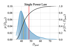
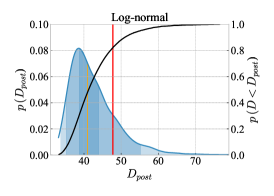
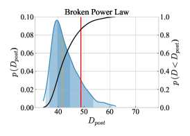
Figure 7 shows the results for each of the three IMF models. In each case the $D_{post,obs}$ falls well within the bulk of the distribution of $D_{post}$. For none of the 3 models the fit is outstandingly better or worse than for the others. All three models are not inconsistent with the data according to our gof test. This confirms the qualitative conclusion that could be drawn from the luminosity functions of Figure 6: all three IMF models can produce CMDs that are consistent with the observed CMD.

Figure 7: Goodness of fit test based on the posterior predictive distribution, $D_{post}$, for each of the three adopted IMF models. The shades of blue in the distributions indicate the 68%, 95% and 99% quantiles, the orange vertical line the median. The black line is the cumulative (right y-axis of each panel). The red line indicates the value of $D_{post}$ for the observed dataset. Since these values are always withing the 95% interval, no model can be rules out by our goodness of fit test.

6.2 Comparison with results from optical data

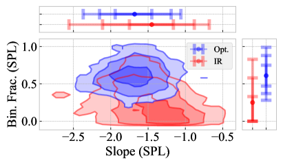
When compared to the results of Gennaro et al. (2018), our current results for the SPL and LN model IMF are in good agreement, namely the SPL slope and the LN $m_{c}$ and $\sigma$ are within the 68% C.I. (see Figure 8). This is an important sanity check for both works, demonstrating that any bias in the results due to the different mass ranges probed, as well as to uncertainties in the adopted color-temperature and/or the mass-luminosity relations, if present, must be negligible with respect to the uncertainties in the parameters estimate.

We cannot perform a comparison for the broken power-law model, since Gennaro et al. (2018) did not attempt a BPL modeling of the IMF to fit their optical data. This was because their data only reach down to $\sim 0.4-0.5\mathrm{~{}M}_{\odot}$ on average for the six galaxies of their sample.

The binary fractions are generally in worse agreement between the current work and Gennaro et al. (2018). The derived binary fraction is quite sensitive to the observed width in the CMD. As illustrated in section 2.5, we were forced to add an extra error in order for our simulated CMDs to reproduce the observed CMD width. We used the same extra error in each band and at all magnitudes, because a more detailed model for it would have implied a better “a priori” knowledge of what the width of the simulated CMD should have looked like, i.e., a knowledge of the binary fraction, among other things. We speculate that the necessarily qualitative-only assessment of the extra errors may have caused an extra spread of the simulated main sequence, which in turn translates into a smaller binary fraction, to compensate for the extra width. On the other end, in Gennaro et al. (2018), Com Ber was the only UFD with a best-fit binary fraction higher than 50%, while for the other UFDs the best fit binary fraction was always smaller than 30%. Thus it could be that the binary fraction was overestimated in that work as well. We do not try to draw further conclusions from a discrepancy between the derived binary fractions.

Figure 8: Comparison of the results for the optical data of ComBer (Gennaro et al., 2018, , blue) and the IR data of the present paper (red). The contour plots show pairwise relations for the Single Power Law (SPL) model parameters, and the Log-Normal (LN) model parameters. The top and left plots in each quadrant show the 68-95-99 % credibility intervals ranges for each parameter, obtained from the respective marginal probability distributions.

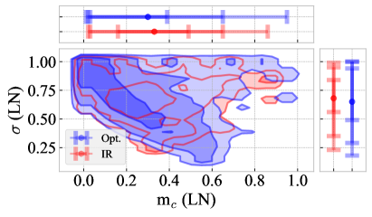
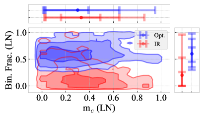
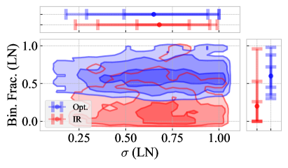
6.3 Comparison with the Milky Way

If limited to the SPL parametrization, our results would suggest that the mean IMF slope of Com Ber is somewhat shallower from the Milky Way classical Salpeter slope of $-2.35$. At the same time, given the limited mass range and the small number of stars (717), the significance of such a result is limited. The Salpeter value falls outside the 95% credible interval, but inside the 99% one.

The BPL and LN parametrizations give results that are more similar to the Milky Way for the same type of functional forms, i.e. Kroupa (2001) for the BPL and Chabrier (2003) or Bochanski et al. (2010) for the LN form. While the best-fit parameters for both the BPL and LN model would result into a slightly bottom lighter IMF for Com Ber with respect to the Galaxy, the Kroupa (2001) and Chabrier (2003) values are within the 68% confidence interval.

Gennaro et al. (2018), based on slope values from SPL model fits, claimed that, on average, a group of 6 UFDs showed a more bottom light IMF with respect to the Milky Way, i.e. fewer dwarf stars. It is possible that the differences between the IMF for the UFDs with respect to the Galaxy claimed by Gennaro et al. (2018) are, at least partly, an artifact of using a SPL model. Gennaro et al. (2018) studied the mass range above 0.4-0.5 M_⊙, at the edge where Kroupa (2001) place the power-law break, and claimed to not expect a significantly biased result for an SPL model. On the other hand, El-Badry et al. (2017) show how adopting a SPL model could artificially lead to shallow slopes if the true underlying IMF has a log-normal shape and data do not probe down to the characteristic mass. El-Badry et al. (2017) obtain a slope of $\sim-1.55$ by fitting a Chabrier (2003) IMF with an SPL model, but limiting the fit to the $(0.4-0.77)$ M_⊙ range, similar to what obtained by Gennaro et al. (2018) for Com Ber. The fact that the results of the current work, for the SPL model, using an extended mass range which reaches very close to the Chabrier (2003) characteristic mass, are very similar to Gennaro et al. (2018) shows however that any bias, if present, must be smaller than the uncertainty introduced by the limited number of stars used.

It is worth noting that in Gennaro et al. (2018) Com Ber was, together with Boo I, the UFD for which the IMF best-fit parameters for both an SPL and LN model were closer to those of the Milky Way. Other galaxies in Gennaro et al. (2018), in particular Hercules, Leo IV and CVn II, showed a much more significant discrepancy, and mean slope values close to $-1$. Also the characteristic mass for the LN model for these three galaxies was much higher than the Chabrier (2003) value, thus for those galaxies the discrepancy with the Milky Way was present even when using the LN parametrization (although, again with lower significance than when using an SPL model).

Gennaro et al. (2018) noted that Com Ber and Boo I, being the closest UFDs in their sample, subtended a larger angle in the sky, and thus their CMDs could have been more contaminated by unresolved background galaxies, specially at the faint end, making their IMF artificially steeper. In the current work we have tried to minimize the impact of background interlopers by limiting ourselves to $m_{160}<28.6$ mag, where we can still discriminate between extended background galaxies and point sources. This does not ensure 100% purity in our sample, and thus may be part of the reason for having an IMF that does not differ from the Milky Way as significantly as for other UFDs.

6.4 The effect of fixing the binary fraction

In Section 6.2 we illustrated some possible concerns on the reliability of the estimated binary fraction, related to the extra error added to our artificial star tests in order to reproduce the observed width of the CMD. With those caveats in mind, it is still interesting to dissect the multi-dimensional posterior probability distribution functions in order to emphasize the correlation of the other parameters with the binary fraction itself.

For each of the SPL, LN and BPL models, we have divided the posterior draws in 4 parts, corresponding to the 0 to 25%, 25% to 50%, 50% to 75% and 75% to 100% quantiles of the marginal distribution of the binary fraction. The edges of the quantiles change slightly between the different models, according to the detailed difference in the marginal distribution of the binary fraction.

Figure 9: Marginal distribution of the fit parameters for different limited to draws corresponding to selected ranges of the binary fraction. Each of the ”range slices” in the binary fraction parameter contains the same number of posterior draws. Each slice, indicated by different colors, corresponds to a 25% quantile. The vertical dashed lines indicate the mean of the corresponding distributions. Top: the SPL case; Center: the LN case; Bottom: the BPL case.

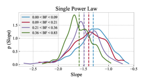
The two parameters that are observed to correlate the most with the binary fraction are the slope in the SPL model and the characteristic mass, $m_{c}$ in the LN model. The correlation goes in the same direction for both models: a smaller binary fraction corresponds to a more bottom-light IMF. At increasingly high binary fraction, the marginal distributions for the slope in the SPL model and $m_{c}$ in the LN model become more consistent with what is observed in the Milky Way. A similar but less prominent correlation is observed for the slopes and the break mass in the BPL case. Even in this case, when considering a higher binary fraction, the IMF becomes more ”bottom-heavy” or more Galaxy-like.

While this is an interesting exercise, we do not have any prior knowledge that allows us to independently constrain the binary fraction, and thus narrow down the uncertainty on the paramters that correlate with it. Our fitting procedure allows us to marginalize over the uncertain binary fraction and report more realistic uncertainties on the other parameters, than if we were to arbitrarely fix them to, e.g. the typical values observed in the Galaxy of about 30% (Raghavan et al., 2010).

A further caveat to consider is the way in which binary pairing is implemented in our simulations. As explained in Gennaro et al. (2018), our IMF represents the distribution of system masses. In simulating synthetic CMDs, we draw system masses, $M_{sys}$, from an IMF model, then decide whether a system should be a single star or a binary, according to a probability set by the binary fraction. If the system is labeled as binary, a mass ratio, $q=M_{2}/M_{1}$, is drawn from a uniform distribution between 0 and 1. Individual masses are given by $M_{1}=\frac{M_{sys}}{1+q}$ and $M_{2}=\frac{qM_{sys}}{1+q}$ . This is different than drawing individual masses from the same IMF and pairing randomly. The qualitative argument for our choice is that it is unlikely that the two stars in a binary are completely independent draws from the same IMF. For progressively tighter binaries it is reasonable to assume that at formation the two stars affected each other’s amount of accreted mass from the protostellar phase.

In determining the mass ratio distribution, we used the fact that for ”solar-type” stars, the binary mass ratio is uniformly distributed between 0 and 1 (Duquennoy & Mayor, 1991; Raghavan et al., 2010). Such a distribution may not be valid outside of the Milky Way or in different mass regimes. We thus stress that, while we use a reasonable assumption, the derived fraction of binaries depends on the adopted mass-ratio distribution.

Nevertheless, we performed a sanity check on the adopted rule of binary component pairing. We verified that our process for generating binaries, which we refer to as correlated draws, does not alter the inferred slope, with respect to a method in which the two stars in a binary are generated from the same single star IMF, referred to as independent draws. We assume the same input slope for the single star IMF and the system IMF in the independent and correlated case respectively. We then compare the single star (primaries plus secondaries), system, as well as the primary star and secondary star distributions. Differences appear at the high and low-end of the mass spectrum. The differences at the low-mass edge are due to the fact that in the correlated case, secondaries can in principle have $M_{2}\rightarrow 0$, while a finite limit must be set for extracting individual masses from a power law in the independent case. At the high-mass edge there are differences due to the definitions of upper limits, i.e., we cannot enforce the same limit on both the maximum individual mass and the maximum system mass consistently for both the independent and correlated scenarios. When limiting the analysis to the mass region accessible to us, i.e., far from both the low-mass and high-mass end of the IMF, no significant differences appear for either the mass ratio distribution, the individual stars distribution, and the system mass distribution between the two methods of generating binaries. As an example, a 2-samples Kolomogorov-Smirnov test for 1000 draws from each of the independent and correlated cases, gives a p-value of 0.95, thus the null-hypothesis that the distributions of the two samples are the same cannot be rejected.

7 Summary and conclusions

We have probed the IMF of the ultra faint dwarf Coma Berenices down to a mass of 0.23 M_⊙, the lowest mass probed to date in a Milky Way satellite, approaching the hydrogen burning limit. Our observation have in fact a deeper limit of about 0.17M_⊙. However the purity of our sample decreases strongly below F160W = 28.6 mag, corresponding to 0.23 M_⊙. This can be attributed to the limited angular resolution of $HST$ in the near-infrared. We fail to distinguish small, faint background galaxies from Com Ber stars below such magnitude.

We have explored three possible IMF parameterizations: Single Power Law (SPL), Broken Power Law (BPL) and Log-normal (LN). Summarizing, we find that:

• the best-fit results for all three IMF parametrization produce similarly good qualitative agreement with the data,

• no strong bias due to the adopted mass range is evident in the result for the SPL or LN model, when compared to the results of Gennaro et al. (2018)

• the SPL model best fit values for Com Ber are marginally consistent with the Milky Way value by Salpeter (1955). The BPL and LN best fits are fully consistent with the Kroupa (2001) and Chabrier (2003) results for the same models for the Milky Way, respectively

We discuss that part of the discrepancy between the Milky Way IMF and that for a sample of 6 UFDs, including Com Ber, claimed in Gennaro et al. (2018) could be related to using a SPL model, which may lead to artificially shallow slopes, if the underlying IMF is a log-normal and if the log-normal characteristic mass is below the probed mass range (see El-Badry et al., 2017). We note however that extending the mass range with respect to Gennaro et al. (2018) down to the Milky Way characteristic mass value (Chabrier, 2003) does not change the slope values significantly. Background contamination could be an additional factor in making the derived Com Ber IMF artificially steeper. On the other end, 3 UFDs in the Gennaro et al. (2018) sample of 6 galaxies show a significantly more bottom-light IMF than Com Ber. This could mean that there is true variance between the UFDs, as quantified by the very different SPL best-fit values, and therefore while some, like Com Ber, might have an IMF consistent with the Milky Way one, others, like CVn II, Hercules and Leo IV, might truly differ from the Galaxy. Moreover the good fit provided by the SPL model for Com Ber indicates that there is no evidence of an IMF turnover, at least with the available number of observed stars.

At this stage we are still gathering evidence on whether the IMF in low-metallicity systems, which formed stars 14 Gyr ago when our Universe was a very different environment, is different from the IMF of stars that are currently forming in our own Galaxy. This leaves the question open for study with future observatories that will become available in the next decade. JWST and WFIRST, above all, will provide both depth to push the probed mass range towards the hydrogen burning limit as well as the field of view to efficiently study nearby, low surface brightness dwarf galaxies; in addition, in the case of JWST, we will be able to exploit the increased angular resolution needed to improve star/galaxy separation at faint limits.

References

- Andersen et al. (2017) Andersen, M., Gennaro, M., Brandner, W., et al. 2017, A&A, 602, A22
- Bastian et al. (2010) Bastian, N., Covey, K. R., & Meyer, M. R. 2010, ARA&A, 48, 339
- Bochanski et al. (2010) Bochanski, J. J., Hawley, S. L., Covey, K. R., et al. 2010, AJ, 139, 2679
- Brammer (2016) Brammer, G. 2016, Reprocessing WFC3/IR Exposures Affected by Time-Variable Backgrounds, Tech. rep.
- Brown et al. (2014) Brown, T. M., Tumlinson, J., Geha, M., et al. 2014, ApJ, 796, 91
- Cappellari et al. (2012) Cappellari, M., McDermid, R. M., Alatalo, K., et al. 2012, Nature, 484, 485
- Cardelli et al. (1989) Cardelli, J. A., Clayton, G. C., & Mathis, J. S. 1989, ApJ, 345, 245
- Chabrier (2003) Chabrier, G. 2003, PASP, 115, 763
- Conroy & van Dokkum (2012) Conroy, C., & van Dokkum, P. G. 2012, ApJ, 760, 71
- Correnti et al. (2016) Correnti, M., Gennaro, M., Kalirai, J. S., Brown, T. M., & Calamida, A. 2016, ApJ, 823, 18
- Da Rio et al. (2012) Da Rio, N., Robberto, M., Hillenbrand, L. A., Henning, T., & Stassun, K. G. 2012, ApJ, 748, 14
- Duquennoy & Mayor (1991) Duquennoy, A., & Mayor, M. 1991, A&A, 248, 485
- El-Badry et al. (2017) El-Badry, K., Weisz, D. R., & Quataert, E. 2017, MNRAS, 468, 319
- Foreman-Mackey (2016) Foreman-Mackey, D. 2016, The Journal of Open Source Software, 24, doi:10.21105/joss.00024. http://dx.doi.org/10.5281/zenodo.45906
- Foreman-Mackey et al. (2013) Foreman-Mackey, D., Hogg, D. W., Lang, D., & Goodman, J. 2013, PASP, 125, 306
- Geha et al. (2013) Geha, M., Brown, T. M., Tumlinson, J., et al. 2013, ApJ, 771, 29
- Gennaro et al. (2015) Gennaro, M., Tchernyshyov, K., Brown, T. M., & Gordon, K. D. 2015, ApJ, 808, 45
- Gennaro & the WFC3 team (2018) Gennaro, M., & the WFC3 team. 2018, WFC3 Data Handbook v. 4.0. http://www.stsci.edu/hst/wfc3/documents/handbooks/currentDHB/wfc3_cover.html
- Gennaro et al. (2018) Gennaro, M., Tchernyshyov, K., Brown, T. M., et al. 2018, ApJ, 855, 20
- Gonzaga et al. (2012) Gonzaga, S., Hack, W., Fruchter, A., & Mack, J. 2012, The DrizzlePac Handbook
- Goodman & Weare (2010) Goodman, J., & Weare, J. 2010, Communications in Applied Mathematics and Computational Science, Vol. 5, No. 1, p. 65-80, 2010, 5, 65
- Gustafsson et al. (2008) Gustafsson, B., Edvardsson, B., Eriksson, K., et al. 2008, A&A, 486, 951
- Hußmann et al. (2012) Hußmann, B., Stolte, A., Brandner, W., Gennaro, M., & Liermann, A. 2012, A&A, 540, A57
- Kalirai et al. (2013) Kalirai, J. S., Anderson, J., Dotter, A., et al. 2013, ApJ, 763, 110
- Kroupa (2001) Kroupa, P. 2001, MNRAS, 322, 231
- Kroupa (2002) —. 2002, Science, 295, 82
- Larson (2005) Larson, R. B. 2005, MNRAS, 359, 211
- Leigh et al. (2012) Leigh, N., Umbreit, S., Sills, A., et al. 2012, MNRAS, 422, 1592
- Lemaire et al. (2016) Lemaire, L., Jay, F., Lee, I., Csilléry, K., & Blum, M. G. B. 2016, ArXiv e-prints, arXiv:1601.04096
- Lyubenova et al. (2016) Lyubenova, M., Martín-Navarro, I., van de Ven, G., et al. 2016, MNRAS, 463, 3220
- Martín-Navarro et al. (2015) Martín-Navarro, I., La Barbera, F., Vazdekis, A., Falcón-Barroso, J., & Ferreras, I. 2015, MNRAS, 447, 1033
- Moraux et al. (2003) Moraux, E., Bouvier, J., Stauffer, J. R., & Cuillandre, J.-C. 2003, A&A, 400, 891
- Muñoz et al. (2010) Muñoz, R. R., Geha, M., & Willman, B. 2010, AJ, 140, 138
- Newman et al. (2017) Newman, A. B., Smith, R. J., Conroy, C., Villaume, A., & van Dokkum, P. 2017, ApJ, 845, 157
- Paust et al. (2010) Paust, N. E. Q., Reid, I. N., Piotto, G., et al. 2010, AJ, 139, 476
- Rafelski et al. (2015) Rafelski, M., Teplitz, H. I., Gardner, J. P., et al. 2015, AJ, 150, 31
- Raghavan et al. (2010) Raghavan, D., McAlister, H. A., Henry, T. J., et al. 2010, ApJS, 190, 1
- Salpeter (1955) Salpeter, E. E. 1955, ApJ, 121, 161
- Schechter (1976) Schechter, P. 1976, ApJ, 203, 297
- Simon & Geha (2007) Simon, J. D., & Geha, M. 2007, ApJ, 670, 313
- Smith (2014) Smith, R. J. 2014, MNRAS, 443, L69
- Sollima & Baumgardt (2017) Sollima, A., & Baumgardt, H. 2017, MNRAS, 471, 3668
- Spiniello et al. (2012) Spiniello, C., Trager, S. C., Koopmans, L. V. E., & Chen, Y. P. 2012, ApJ, 753, L32
- Stetson (1987) Stetson, P. B. 1987, PASP, 99, 191
- van Dokkum et al. (2017) van Dokkum, P., Conroy, C., Villaume, A., Brodie, J., & Romanowsky, A. J. 2017, ApJ, 841, 68
- van Dokkum & Conroy (2010) van Dokkum, P. G., & Conroy, C. 2010, Nature, 468, 940
- van Dokkum & Conroy (2011) —. 2011, ApJ, 735, L13
- van Dokkum & Conroy (2012) —. 2012, ApJ, 760, 70
- VandenBerg et al. (2014) VandenBerg, D. A., Bergbusch, P. A., Ferguson, J. W., & Edvardsson, B. 2014, ApJ, 794, 72
- Vesperini & Heggie (1997) Vesperini, E., & Heggie, D. C. 1997, MNRAS, 289, 898
- Webb et al. (2017) Webb, J. J., Vesperini, E., Dalessandro, E., et al. 2017, MNRAS, 471, 3845
- Weisz et al. (2013) Weisz, D. R., Fouesneau, M., Hogg, D. W., et al. 2013, ApJ, 762, 123
- Wyse et al. (2002) Wyse, R. F. G., Gilmore, G., Houdashelt, M. L., et al. 2002, New A, 7, 395