Simultaneous model calibration and source inversion in atmospheric dispersion models

Abstract

We present a cost-effective method for model calibration and solution of source inversion problems in atmospheric dispersion modelling. We use Gaussian process emulations of atmospheric dispersion models within a Bayesian framework for solution of inverse problems. The model and source parameters are treated as unknowns and we obtain point estimates and approximation of uncertainties for sources while simultaneously calibrating the forward model. The method is validated in the context of an industrial case study involving emissions from a smelting operation for which cumulative monthly measurements of zinc particulate depositions are available.

1 Introduction

This article presents a methodology for simultaneously estimating pollutant emission rates and calibrating atmospheric dispersion models using far-field measurements of particulate deposition. We use a Gaussian process (GP) emulator to efficiently approximate a relatively expensive partial differential equation (PDE) model for atmospheric dispersion which is then coupled with a Bayesian framework for source inversion and uncertainty quantification.

Source identification (or inversion) problems are prevalent in various areas of environmental monitoring kim2007advanced and forensics mudge2008environmental . These problems are often difficult to solve due to the scarcity of data and the complexity of physical processes that obscure the true nature of sources. Traditionally, source identification problems are solved by a combination of empirical techniques such as chemical analysis morrison2000application , remote sensing methods like thermal imaging matson1981identification , and statistical tools such as principle component analysis mudge2007multivariate . Owing to the prevalence of measurement methods and chemical analysis in the forensics literature colbeck2009 ; hesterharrison2008 ; spikmans2019forensics , the application of mathematical models and numerical simulations is relatively under-developed. This is in part due to complexity of certain mathematical models, uncertainty in values of tuning parameters, and general difficulty in assessing confidence in simulations. And even when the errors and uncertainties in contaminant measurements may be well-known or controlled, the effect of those errors when they are used as inputs for a source inversion model is much less well understood. It is therefore crucial to quantify the effect of measurement errors on emissions estimates and obtain uncertainty bounds in order to make reliable and defensible claims in forensics applications.

In the context of atmospheric pollutant dispersion, numerous mathematical models are available that provide approximations to the actual physical processes driving dispersion of particulates and other substances within the atmosphere chatwin1982use ; lewellen1989meteorological . A common challenge in dispersion modelling is to maintain accuracy since many models suffer from sizable errors and large uncertainties in parameters. In some cases, these inaccuracies can be addressed by increasing the model complexity to account for physical processes that have been neglected, in the hope that the resulting more complex model yields correspondingly higher accuracy and more realistic simulations. However, in many practical applications, such extensions lead to no significant improvement in the solution because the model errors are far outweighed by the uncertainty in values of the model parameters. This difficulty is further exacerbated by the fact that many models contain a large number of unknown model parameters. Some of these parameters have a clear physical basis, such as diffusion coefficients, particulate density and settling velocities, whereas others are mathematical (or fitting) parameters such as the Monin-Obukhov length, atmospheric stability classes, or terrain roughness length.

Direct measurements of many physical and mathematical parameters are often problematic or even infeasible; for example, eddy diffusion coefficients are typically difficult to estimate in practice seinfeld1998atmospheric . One is therefore often forced to deal with significant uncertainties in the true value of model parameters, even when complex models are employed that under ideal circumstances could potentially simulate results very accurately. Because large errors in model parameters can severely contaminate simulations, it is therefore essential when simulating atmospheric dispersion scenarios to simultaneously understand and control the parameter uncertainty. Sources of uncertainty are diverse and can be classified roughly into one of three types rao2005uncertainty :

• Data uncertainty: when the empirical measurements or model parameter values are inaccurate;

• Model uncertainty: where the model does not capture all physical processes of interest; or

• Stochastic uncertainty: relating to the inherent unpredictability or randomness in physical processes, such as atmospheric turbulence.

In this work we focus primarily on dealing with the first case of data uncertainty appearing in the context of atmospheric source inversion problems.

Despite the difficulty of obtaining accurate simulations, there is a growing need to develop more accurate and computationally efficient models for practical atmospheric dispersion applications leelHossy2014dispersion . The necessity for computational efficiency comes from the fact that models for atmospheric transport are usually expressed as systems of partial differential equations that are computationally expensive to solve at the typical resolutions required, which is a particular limitation for real-time applications. Efficiency is of even greater importance in the context of source inversion problems, since a single solution of the inverse problem may require a large number of evaluations of the forward dispersion model. One of the goals of this work is therefore to demonstrate how to use computationally demanding forward models to solve atmospheric source inversion problems in an efficient manner.

1.1 Atmospheric dispersion modelling

We model the dispersion of pollutants in the atmosphere using the advection-diffusion PDE

$$\frac{\partial C(\textbf{x},t)}{\partial t}+\nabla\cdot(\bar{\textbf{v}}C(\textbf{x},t)-\textbf{D}\nabla C(\textbf{x},t))=f(\textbf{x},t),$$ (1)

where $C(\textbf{x},t)$ denotes the concentration of pollutant at location $\textbf{x}=(x,y,z)\in\mathbb{R}^{3}$, $t$ is time, $\bar{\textbf{v}}$ is the wind velocity field, D is the diffusivity tensor, and $f(\textbf{x},t)$ is a pollutant source term. Throughout this paper we always consider (1) with zero initial condition $C(\textbf{x},0)=0$, so that no pre-existing transient concentrations exist. We make this assumption for reasons of simplicity, and because in practice it is often very difficult to measure these pre-existing concentrations. We focus on the case of a finite collection of $n$ point sources each having an emission rate that is constant in time, which allows $f$ to be written as

$$f(\textbf{x},t)=\sum_{j=1}^{n}q_{j}\delta(\textbf{x}-\textbf{x}_{j}),$$ (2)

where $\textbf{q}=(q_{1},q_{2},\ldots,q_{n})^{T}\in\mathbb{R}^{n}$ represent emission rates, $\{\textbf{x}_{j}\}_{j=1}^{n}$ are the locations of the sources, and $\delta(\textbf{x}-\textbf{x}_{j})$ are Dirac delta functions representing point sources at the locations $\textbf{x}_{j}$. The wind velocity field $\bar{\textbf{v}}$ and diffusivity tensor D are often difficult to measure and so are replaced using simpler mathematical approximations that depend upon empirical parameters describing the variation of $\bar{\textbf{v}}$ and D with time and space. Common examples of such parameters include roughness length, Monin-Obukhov length and Pasquill stability class seinfeld1998atmospheric . We combine all empirical parameters together into a vector $\boldsymbol{\theta}=(\theta_{k})\in\mathbb{R}^{m}$, and then denote the linear operator $\nabla\cdot(\textbf{v}+\textbf{D}\nabla)$ on the left hand side of $\eqref{eqnModelIntro}$ by $\textbf{L}(\boldsymbol{\theta})$ to make explicit the dependence of the operator on the parameter vector $\boldsymbol{\theta}$, noting that the dependence of L on $\boldsymbol{\theta}$ can still be nonlinear. Then we rewrite (1) as

$$\frac{\partial C(\textbf{x},t)}{\partial t}+\textbf{L}(\boldsymbol{\theta})C(\textbf{x},t)=\sum_{j=1}^{n}q_{j}\delta(\textbf{x}-\textbf{x}_{j}).$$ (3)

The task of finding the concentration $C(\textbf{x},t)$ given q and $\boldsymbol{\theta}$, supplemented by suitable boundary and initial conditions, is referred to as the forward problem in the context of atmospheric pollutant transport.

1.2 Atmospheric source inversion

The goal of atmospheric source inversion is to estimate the source term $f(\textbf{x},t)$ on the right hand side of (1) from indirect measurements of the concentration $C(\textbf{x},t)$. We consider equation (3) with a set of given point sources at known locations, but with unknown constant emission rates. Our aim is then to estimate the emission rates $q_{j}$ from indirect measurements of $C(\textbf{x},t)$. To this end, the source inversion problem is the reverse of the forward problem (3) and is thus an inverse problem.

We assume that measurements of concentration can be treated in terms of the action of bounded linear operators on $C$. For example, a common measurement in particulate dispersion studies is the total accumulated deposition of pollutants in a region $R\subset\mathbb{R}^{2}$ of the ground surface after some time $T$ has elapsed. Such a measurement can be written as

$$\int_{R}\int_{0}^{T}C(x,y,0,t)v_{\textit{set}}\,dt\,dx\,dy,$$

where $v_{\textit{set}}$ is the vertical settling velocity at the ground surface for the pollutant of interest. The class of all possible linear measurements is large and includes many commonly used methods in practice ranging from short time average measurements such as Xact ambient metal monitors cooper-environmental-2015 and Andersen high-volume air samplers thermo-scientific-2015 , as well as averaged long-time measurements accumulated in dustfall jars.

Suppose now that field measurements of $C$ are taken at $d$ locations in space and collected in a vector $\textbf{w}\in\mathbb{R}^{d}$. Since the measurements are linear, we can write

$$\textbf{w}=\mathcal{A}(\boldsymbol{\theta})\,\textbf{q},$$ (4)

where $\mathcal{A}(\boldsymbol{\theta})$ is a $d\times n$ matrix that represents the solution map of the PDE (3) and depends nonlinearly on the model parameters $\boldsymbol{\theta}$. Source inversion requires finding q given w, and it is well known that this problem is ill-posed in the sense of Hadamard enting1990inverse ; isakov1990inverse ; that is, small variations in the inputs (w) result in large variations in the solution (q). This is the case even if the true value of $\boldsymbol{\theta}$ is known exactly.

A variety of different approaches have been proposed in the literature to solve source inversion problems haupt-young-2008 ; rao-2007 . Lin and Chang lin2002relative used an air trajectory statistical approach to estimate the strength of different sources of volatile organic compounds of anthropogenic origin. Stockie and Lushi lushi2010inverse used a Gaussian plume approximation to the governing PDEs to estimate ground-level deposition of zinc from a lead-zinc smelter, using linear least-squares to perform the source inversion. Skiba skiba2003method solved the adjoint equation for the advection-diffusion equation and used penalized least-squares to invert the sources.

All of the methods just mentioned yield point estimates for the source strengths but provide no direct measure of uncertainty in the estimated parameters. This drawback is overcome by the use of probabilistic methods such as the Bayesian approach for solving inverse problems. Such methods provide a robust setting for solving the inverse problem and quantifying the uncertainties associated with the solution. Sohn et al. sohn2002rapidly developed an algorithm to obtain estimates and uncertainties for the location and strength of pollutant sources in buildings using data obtained from a COMIS simulation. Hosseini and Stockie hosseini2016bayesian used a Gaussian plume model combined with experimental data to estimate and quantify the uncertainty of airborne fugitive emissions. In a follow-up publication hosseini2016airborne , the same authors coupled a Bayesian approach with a finite volume solver to estimate and quantify the strength of airborne contaminants from a fixed number of point sources at known locations. Keats et al. keats2007bayesian obtained probability distributions for source strengths and locations using data from the standard “Muck Urban Setting Test” experiment.

The central contribution of this work is in proposing a method that deals with the calibration parameters $\boldsymbol{\theta}$ as unknowns. We infer $\boldsymbol{\theta}$ along with the vector of source strengths q, which results in a nonlinear inverse problem that is solved within the Bayesian framework. The problem of estimating the true value of the parameters $\boldsymbol{\theta}$ is referred to as model calibration. Traditionally, the process of tuning parameters in atmospheric dispersion models is done empirically using Pasquill stability classes turner1994workbook ; seinfeld1998atmospheric that are often chosen heuristically. Instead, we automatically estimate these parameters using the information contained in the measured data w.

1.3 Outline

The remainder of this article is organized as follows: In Section 2 we introduce GP emulators for approximation of computationally expensive models. Section 3 is dedicated to the Bayesian framework for simultaneous calibration of the model and solution of the source inversion problem. In Section 4 we apply our framework for emulation and calibration to an industrial case study involving air-borne particulate emissions from a lead-zinc smelter in Trail, British Columbia, Canada and compare our results with previous studies and engineering estimates.

2 Emulation of atmospheric dispersion models

In this section we introduce a framework for emulation of atmospheric dispersion models using GPs. Equation (3) captures the linear relationship between source strengths $\textbf{q}\in\mathbb{R}^{n}$ and concentration $C(\textbf{x},t)$. Under the further assumption that the data $\textbf{w}\in\mathbb{R}^{d}$ also depends linearly on concentration $C(\textbf{x},t)$, we can write the map $\textbf{q}\mapsto\textbf{w}$ in the linear form (4), although we note that in general, $\mathcal{A}(\boldsymbol{\theta})\in\mathbb{R}^{d\times n}$ may depend nonlinearly on $\boldsymbol{\theta}\in\mathbb{R}^{m}$. Therefore, the map $(\textbf{q},\boldsymbol{\theta})\mapsto\textbf{w}$ can be split into two parts: for fixed values of $\boldsymbol{\theta}$ the map $(\cdot,\boldsymbol{\theta})\mapsto\textbf{w}$ is linear, whereas for a fixed q the mapping $(\textbf{q},\cdot)\mapsto\textbf{w}$ is nonlinear. We will exploit this structure in the design of our source inversion algorithm, using the fact that the linear map $(\cdot,\boldsymbol{\theta})\mapsto\textbf{q}$ can be dealt with efficiently, but that we will need to approximate the nonlinear map $(\textbf{q},\cdot)\mapsto\textbf{w}$.

To this end, we approximate the matrix

$$\mathcal{A}(\boldsymbol{\theta})=[\mathfrak{a}_{ij}(\boldsymbol{\theta})]\in\mathbb{R}^{d\times n},$$ (5)

with another matrix

$$A(\boldsymbol{\theta})=[a_{ij}(\boldsymbol{\theta})]\in\mathbb{R}^{d\times n},$$

where each entry $\mathfrak{a}_{ij}:\mathbb{R}^{m}\mapsto\mathbb{R}$ of $\mathcal{A}$ is approximated by the map $a_{ij}:\mathbb{R}^{m}\mapsto\mathbb{R}$. For this purpose, we make use of GP emulators of kennedy2001bayesian . Emulation with GPs is a well-established method in dynamic computer experiments and machine learning and we refer the reader to rasmussen2006gaussian ; kennedy2001bayesian ; o2006bayesian ; conti2009gaussian and the references within for an introduction to this subject. Here, we outline our method for approximating $\mathcal{A}$ and will not discuss the theory of GP emulators with the exception of a few crucial definitions and results.

Definition 1

A GP on $\mathbb{R}^{m}$ is a collection of real-valued random variables $\{g(\mathbf{x})\}_{\mathbf{x}\in\mathbb{R}^{m}}$, any finite collection of which have a joint Gaussian distribution.

We denote a GP using the notation

$$g\sim\mathcal{GP}(\bar{g},\kappa),$$

where the mean of the GP is

$$\bar{g}(\boldsymbol{\theta})=\mathbb{E}\>g(\boldsymbol{\theta})\qquad\forall\boldsymbol{\theta}\in\mathbb{R}^{m},$$

and $\kappa$ is a positive semi-definite kernel with

$$\kappa(\boldsymbol{\theta},\boldsymbol{\theta}^{\prime})=\mathbb{E}\>(g(\boldsymbol{\theta})-\bar{g}(\boldsymbol{\theta}))(g(\boldsymbol{\theta}^{\prime})-\bar{g}(\boldsymbol{\theta}^{\prime}))\qquad\forall\boldsymbol{\theta},\boldsymbol{\theta}^{\prime}\in\mathbb{R}^{m}.$$

We are primarily interested in isotropic kernels that satisfy

$$\kappa(\boldsymbol{\theta},\boldsymbol{\theta}^{\prime})=\kappa(|\boldsymbol{\theta}-\boldsymbol{\theta}^{\prime}|),$$

from which it follows that if $\bar{g}$ is continuous and $\kappa$ is continuous at zero, then the GP is also mean square continuous rasmussen2006gaussian .

Let $\{\boldsymbol{\theta}_{k}\}_{k=1}^{K}$ be a collection of design points in the parameter space $\mathbb{R}^{m}$ for some fixed $K>0$, and let $\{\mathbf{e}_{j}\}_{j=1}^{n}$ be the unit coordinate basis vectors in $\mathbb{R}^{n}$. Then for each index pair $(i,j)$ define a GP

$$g_{ij}\sim\mathcal{GP}(\bar{g}_{ij},\kappa_{ij}),$$

subject to the constraint

$$g_{ij}(\boldsymbol{\theta}_{k})=\mathfrak{a}_{ij}(\boldsymbol{\theta}_{k})=(\mathcal{A}(\boldsymbol{\theta}_{k})\mathbf{e}_{j})_{i}\qquad\text{for }k=1,\ldots,K.$$

That is, each $g_{ij}$ interpolates the $\mathfrak{a}_{ij}$ at points $\{\boldsymbol{\theta}_{k}\}_{k=1}^{K}$. We can now identify $g_{ij}$ using well-known identities for conditioning of Gaussian random variables (rasmussen2006gaussian, , Sec. 2.2). Let $\Theta:=(\boldsymbol{\theta}_{1},\ldots,\boldsymbol{\theta}_{K})^{T}$ and define the following matrices and vectors

$$G_{ij}(\Theta,\Theta)\in\mathbb{R}^{K\times K},\qquad [G_{ij}(\Theta,\Theta)]_{k\ell}:=\kappa_{ij}(\boldsymbol{\theta}_{k},\boldsymbol{\theta}_{\ell}),$$

$$G_{ij}(\boldsymbol{\theta},\Theta)\in\mathbb{R}^{1\times K},\qquad [G_{ij}(\boldsymbol{\theta},\Theta)]_{\ell}:=\kappa_{ij}(\boldsymbol{\theta},\boldsymbol{\theta}_{\ell}),$$

$$G_{ij}(\Theta,\boldsymbol{\theta})\in\mathbb{R}^{K\times 1},\qquad [G_{ij}(\Theta,\boldsymbol{\theta})]_{k}:=\kappa_{ij}(\boldsymbol{\theta}_{k},\boldsymbol{\theta}),$$

$$\mathbf{g}_{ij}\in\mathbb{R}^{K\times 1},\qquad [\mathbf{g}_{ij}]_{k}=\mathfrak{a}_{ij}(\boldsymbol{\theta}_{k}),$$

for $k,\ell=1,\ldots,K$. Then we have

$$g_{ij}(\boldsymbol{\theta})\sim\mathcal{GP}(\bar{g}_{ij}(\boldsymbol{\theta}),\sigma_{ij}(\boldsymbol{\theta})),$$

where

$$\bar{g}_{ij}(\boldsymbol{\theta}) =G_{ij}(\boldsymbol{\theta},\Theta)G_{ij}(\Theta,\Theta)^{-1}\mathbf{g}_{ij},$$

$$\sigma_{ij}(\boldsymbol{\theta}) =\kappa_{ij}(\boldsymbol{\theta},\boldsymbol{\theta})-G_{ij}(\boldsymbol{\theta},\Theta)\,\left[G_{ij}(\Theta,\Theta)^{-1}\right]G_{ij}(\Theta,\boldsymbol{\theta}),$$

for all $\boldsymbol{\theta}\in\mathbb{R}^{m}$. Since the mean $\bar{g}_{ij}$ interpolates the data $\mathfrak{a}_{ij}(\boldsymbol{\theta}_{k})$, it is also a good candidate for approximating $\mathfrak{a}_{ij}$, and so we take

$$a_{ij}(\boldsymbol{\theta})=\bar{g}_{ij}(\boldsymbol{\theta})\qquad\forall\boldsymbol{\theta}\in\mathbb{R}^{m}.$$

The advantage of using this approach for interpolation is that it is possible to assess the uncertainty and quality of the emulator via the covariance operator $\sigma(\boldsymbol{\theta})$.

The variance at a point $\boldsymbol{\theta}_{i}$ is given by the term $\sigma_{ii}(\boldsymbol{\theta})$ and is strongly influenced by the spatial distribution of the points $\{\boldsymbol{\theta}_{k}\}_{k=1}^{K}$ johnson1990minimax . Thus, in order to emulate $\mathcal{A}(\boldsymbol{\theta})$, it is crucial to choose the points $\boldsymbol{\theta}_{k}$ in such a way that the uncertainty of the emulator is minimized. A popular method for choosing the design points is known as a space-filling design johnson1990minimax , instances of which include the maximum entropy design maxEntDesign , uniform design Fang , and Latin Hypercube design (LHD) LHD . Following Jones et al. jones we use a combination of the LHD and maximin designs, which is introduced in johnson1990minimax and shown to outperform most space-filling design methods for GP interpolation.

We now briefly outline our space-filling design procedure. The main idea in the LHD is to distribute design points such that low-dimensional projections of the points do not overlap. One issue with LHD is that it does not have desirable space-filling properties and so leads to large uncertainties in the emulator in high dimensions. Thus, LHD is often used as an initial condition for other space-filling design methodologies and so here we complement the LHD with an approximate maximin design johnson1990minimax .

The idea behind the maximin design is as follows. Let $T\subset\mathbb{R}^{n}$ be the subset of parameter space in which we wish to construct our design points and consider all subsets $S$ of $T$ with finite (fixed) cardinality, say $|S|=k$. A maximin design $S^{o}$ is a set of points that satisfies

$$\max_{S\subset T,\text{ }|S|=k}\;\min_{s,s^{\prime}\in S}d(s,s^{\prime})=\min_{s,s^{\prime}\in S^{o}}d(s,s^{\prime}),$$ (6)

where $d$ is the Euclidean metric. The optimization problem in equation (6) is not easily solvable, which is why we resort to metaheuristic optimization procedures. In particular, we use the particle swarm algorithm arora2015optimization , initiated with an LHD. We then apply a number of iterations of particle swarm that is chosen depending on our available computational budget. In Figure 3 we show an example of the final design after 10,000 steps of a particle swarm algorithm.

3 The Bayesian inversion framework

We introduce the Bayesian framework for calibration and solution of inverse problems in this section. The Bayesian approach combines the data w together with prior knowledge to give a posterior probability distribution on the source strengths q and calibration parameters $\boldsymbol{\theta}$. Following Bayes’ rule, the posterior distribution of $(\boldsymbol{\theta},\textbf{q})$ is given by

$$\mathbb{P}_{\textit{post}}(\boldsymbol{\theta},\textbf{q}|\textbf{w})=\frac{\mathbb{P}_{\textit{like}}(\textbf{w}|\boldsymbol{\theta},\textbf{q})\,\mathbb{P}_{\textit{prior}}(\boldsymbol{\theta},\textbf{q})}{Z(\textbf{w})},$$ (7)

where $\mathbb{P}_{\textit{like}}(\textbf{w}|\boldsymbol{\theta},\textbf{q})$ is the likelihood probability of w given both $\boldsymbol{\theta}$ and q, which represents the probability of observing w given fixed values q and $\boldsymbol{\theta}$. The probability distribution $\mathbb{P}_{\textit{prior}}(\boldsymbol{\theta},\textbf{q})$ is called the prior probability that expresses prior knowledge of the possible values of q and $\boldsymbol{\theta}$, before observing any experimental data. Finally, $Z(\textbf{w})$ is a constant that normalizes the posterior probability so that it integrates to one, leading to the requirement that

$$Z(\textbf{w})=\int\mathbb{P}_{\textit{like}}(\textbf{w}|\boldsymbol{\theta},\textbf{q})\,\mathbb{P}_{\textit{prior}}(\boldsymbol{\theta},\textbf{q})\,d\boldsymbol{\theta}\,d\textbf{q}.$$ (8)

We next assume that the linearity requirement (4) holds for physical measurements up to some additive Gaussian measurement noise, so that

$$\textbf{w}=\mathcal{A}(\boldsymbol{\theta})\textbf{q}+\epsilon\quad\text{with}\quad\epsilon\sim\mathcal{N}(0,\Sigma).$$ (9)

Here, $\epsilon$ is a normally distributed random vector with mean zero and covariance $\Sigma\in\mathbb{R}^{d\times d}$, which is assumed positive-definite. The measurement noise $\epsilon$ models the deviations in the measurements w due to missing physics and uncertainty in measurements. Under this assumption, it can be readily shown that (Somersalo, , Sec. 3.2.1)

$$\mathbb{P}_{\textit{like}}(\textbf{w}|\boldsymbol{\theta},\textbf{q})=\frac{1}{(2\pi\text{det}\Sigma)^{\frac{1}{2}}}\exp\left(-\frac{1}{2}\left\|\Sigma^{-1/2}(\mathcal{A}(\boldsymbol{\theta})\textbf{q}-\textbf{w})\right\|^{2}\right).$$ (10)

The choice of the prior distribution depends on previous knowledge about the model parameters and so is problem specific. For atmospheric dispersion models, the parameter $\boldsymbol{\theta}$ often depends on atmospheric conditions, whereas the emission rates in the vector q depend on the physical processes that generated the emissions. Consequently, it is reasonable to assume a priori that q and $\boldsymbol{\theta}$ are statistically independent, so that

$$\mathbb{P}_{\textit{prior}}(\boldsymbol{\theta},\textbf{q})=\mathbb{P}_{\textit{prior}}(\boldsymbol{\theta})\,\mathbb{P}_{\textit{prior}}(\textbf{q}).$$ (11)

In most cases, one chooses a prior for q that imposes a positivity constraint on the emission rates, whereas priors on $\boldsymbol{\theta}$ typically reflect acceptable ranges of calibration parameters. Beyond these assumptions, the choice of the prior density for $\boldsymbol{\theta}$ and q must be made on a case by case basis. In Section 4, we present a particular prior distribution for $(\boldsymbol{\theta},\textbf{q})$ in the context of an industrial case study.

A key step in our source inversion approach is approximating the posterior probability $\mathbb{P}_{\textit{post}}$ through an approximation for the map $\mathcal{A}$. Let $A$ be the GP emulator for $\mathcal{A}$ as outlined in Section 2, then we can approximate the likelihood $\mathbb{P}_{\textit{like}}$ in (10) using

$$\widehat{\mathbb{P}_{\textit{like}}}(\textbf{w}|\boldsymbol{\theta},\textbf{q})=\frac{1}{(2\pi\text{det}\Sigma)^{\frac{1}{2}}}\exp\left(-\frac{1}{2}\left\|\Sigma^{-1/2}({A}(\boldsymbol{\theta})\textbf{q}-\textbf{w})\right\|^{2}\right).$$ (12)

Substituting this expression into Bayes’ rule (7) yields the approximate posterior

$$\widehat{\mathbb{P}_{\textit{post}}}(\boldsymbol{\theta},\textbf{q}|\textbf{w})=\frac{\widehat{\mathbb{P}_{\textit{like}}}(\textbf{w}|\boldsymbol{\theta},\textbf{q})\,\mathbb{P}_{\textit{prior}}(\boldsymbol{\theta},\textbf{q})}{\widehat{Z}(\textbf{w})},$$ (13)

where the constant $\widehat{Z}$ is defined similar to (8). If the map $A$ approximates $\mathcal{A}$ closely, then we expect $\widehat{\mathbb{P}_{\textit{post}}}$ to be close to $\mathbb{P}_{\textit{post}}$. We refer the reader to stuart2018posterior and references therein for a detailed analysis of the errors introduced through GP emulation of forward maps in Bayesian inverse problems.

With $\widehat{\mathbb{P}_{\textit{post}}}$ in hand we may now compute point value estimators for the parameters $\boldsymbol{\theta}$ and source strengths q. Common choices of point estimates are Somersalo :

Maximum a posteriori: $$(\boldsymbol{\theta},\textbf{q})_{\textit{MAP}} =\mathop{\mathrm{argmax}}_{\boldsymbol{\theta},\textbf{q}}\,\widehat{\mathbb{P}_{\textit{post}}}(\textbf{w}|\boldsymbol{\theta},\textbf{q}),$$ (14)

Conditional mean: $$(\boldsymbol{\theta},\textbf{q})_{\textit{CM}} =\int(\boldsymbol{\theta},\textbf{q})\,\widehat{\mathbb{P}_{\textit{post}}}(\boldsymbol{\theta},\textbf{q}|\textbf{w})\,d\boldsymbol{\theta}\,d\textbf{q},$$ (15)

Maximum likelihood: $$(\boldsymbol{\theta},\textbf{q})_{\textit{ML}} =\mathop{\mathrm{argmax}}_{\boldsymbol{\theta},\textbf{q}}\,\widehat{\mathbb{P}_{\textit{post}}}(\boldsymbol{\theta},\textbf{q}|\textbf{w}).$$ (16)

The uncertainty in the choice of point estimate $(\boldsymbol{\theta}^{\ast},\textbf{q}^{\ast})$ can be assessed by computing the covariance matrix

$$\int\left((\boldsymbol{\theta},\textbf{q})-(\boldsymbol{\theta}^{\ast},\textbf{q}^{\ast})\right)\otimes\left((\boldsymbol{\theta},\textbf{q})-(\boldsymbol{\theta}^{\ast},\textbf{q}^{\ast})\right)\,\widehat{\mathbb{P}_{\textit{post}}}(\boldsymbol{\theta},\textbf{q}|\textbf{w})\,d\boldsymbol{\theta}\,d\textbf{q}.$$

The above estimators may of course also be computed using the true posterior ${\mathbb{P}_{\textit{post}}}$, but if $\widehat{\mathbb{P}_{\textit{post}}}$ is close to $\mathbb{P}_{\textit{post}}$ in an appropriate sense (such as the total variation metric) then one expects the point estimators under $\widehat{\mathbb{P}_{\textit{post}}}$ to approximate their counterparts under $\mathbb{P}_{\textit{post}}$ stuart2018posterior .

In general, the integrals involved in computing point estimates or covariances are not analytically tractable and so it is necessary to resort to numerical methods for their estimation. Since these are high-dimensional integrals, quadrature-based approaches are unsuitable, thus it is necessary to use Markov chain Monte Carlo (MCMC) integration techniques. In this paper we use the adaptive MCMC algorithm of haario2001 , which is outlined below in Algorithm 1. Specific values of the algorithmic parameters ($\beta_{1}$, $\gamma_{1}$, $\gamma_{2}$, $\gamma_{3}$) that are tailored to our case study are provided later in Section 4.3.

Algorithm 1 Adaptive Metropolis-Hastings Algorithm.

1:Choose $(\boldsymbol{\theta}_{1},\textbf{q}_{1})\in\mathbb{R}^{d}$ in the support of $\mathbb{P}_{\textit{post}}(\boldsymbol{\theta},\textbf{q}|\textbf{w})$ and fixed parameters $\beta\in(0,1)$, $\gamma_{1},\gamma_{2},\gamma_{3}\in(0,\infty)$, $N\in\mathbb{N}$.

2:for $j=2:N$ do

3:     if $j\leq 2d$ then

4:         Draw $u$ from $\mathcal{N}\left((\boldsymbol{\theta}_{j},\textbf{q}_{j}),\frac{\gamma_{1}}{d}I_{d\times d}\right)$.

5:     else

6:         Estimate the empirical covariance matrix $\Sigma_{j}$ using $\{(\boldsymbol{\theta}_{k},\textbf{q}_{k})\}_{k=1}^{j}$.

7:         Draw $u$ from $(1-\beta)\,\mathcal{N}\left((\boldsymbol{\theta}_{j},\textbf{q}_{j}),\frac{\gamma_{2}}{d}\Sigma_{j}\right)+\beta\mathcal{N}\left((\boldsymbol{\theta}_{j},\textbf{q}_{j}),\frac{\gamma_{3}}{d}I_{d\times d}\right)$.

8:     end if

9:     Propose $(\tilde{\boldsymbol{\theta}}_{j},\tilde{\textbf{q}}_{j})=(\boldsymbol{\theta}_{j-1},\textbf{q}_{j-1})+u$.

10:     Compute $\delta=\min\left(1,\frac{\widehat{\mathbb{P}_{\textit{post}}}(\boldsymbol{\theta}_{j},\textbf{q}_{j}|\textbf{w})}{\widehat{\mathbb{P}_{\textit{post}}}(\boldsymbol{\theta}_{j-1},\textbf{q}_{j-1}|\textbf{w})}\right)$.

11:     Draw $w$ from $U([0,1])$.

12:     if $w<\delta$ then

13:         $(\boldsymbol{\theta}_{j},\textbf{q}_{j})=(\tilde{\boldsymbol{\theta}}_{j},\tilde{\textbf{q}}_{j})\qquad\qquad$ (Accept the move)

14:     else

15:         $(\boldsymbol{\theta}_{j},\textbf{q}_{j})=(\boldsymbol{\theta}_{j-1},\textbf{q}_{j-1})\qquad$ (Reject the move)

16:     end if

17:end for

4 An industrial case study

In this section we apply our Bayesian framework to the study of dispersion of airborne zinc particles from four point sources located within the area surrounding a lead-zinc smelter in Trail, British Columbia, Canada. In Section 4.1 we perform a sensitivity analysis that reveals which parameters are most informed by the data. Section 4.2 is dedicated to validating the emulator while Section 4.3 contains the main results for the industrial case study including comparisons with previous studies. Finally, Sections 4.4 and 4.5 provide further validation of our source inversion results and study the dependence of emission estimates and uncertainties on the choice of the priors and quality of the emulator respectively. The methodology of this section was validated in (garcia2018parameter, , Sec. 2) for a synthetic example, and the dependence of the posterior on the number of measurements and choice of the prior distribution was studied in detail.

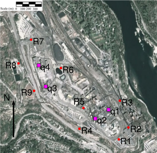
Our ultimate goal is to estimate the contribution that each source makes to the total zinc released into the atmosphere by the smelting operation. We begin by outlining the details of our model and the parameters to be calibrated. We have access to monthly cumulative measurements of zinc particulate depositions at nine separate locations as well as horizontal wind field velocity data at a meteorological station located near the sources. We also have access to engineering estimates of the yearly-averaged emission rates obtained from independent engineering studies based on process control arguments. An aerial photograph of the industrial site, showing the locations of all sources and measurement devices, is provided in Figure 1. The sources are labelled $q_{1}$ to $q_{4}$, and deposition measurements are designated $R_{1}$ to $R_{9}$. This same emission scenario has been studied using a linear least squares approach based on a Gaussian plume approximation lushi2010inverse , and also by performing a finite volume discretization of the governing equation (3) hosseini2016airborne .

Figure 1: Aerial photograph of the lead-zinc smelter in Trail, BC, Canada. The square points labelled ’qn’ represent the locations of the four zinc sources, while the circular points ’Ri’ denote the nine measurement devices.

We apply the atmospheric dispersion model (3), as adapted in hosseini2016airborne for this specific zinc smelter site with $n=4$ sources:

$$\frac{\partial C(\textbf{x},t)}{\partial t}+\textbf{L}(p,z_{0},z_{i},L,z_{\textit{cut}})C(\textbf{x},t)=\sum_{j=1}^{4}q_{j}\delta(\textbf{x}-\textbf{x}_{j}).$$ (17)

The differential operator L depends non-linearly on five parameters as we shall explain next. The parameter $p$ comes from the assumption of a power-law distribution in the vertical component of the wind profile v; that is, if $z$ denotes the height above ground level $(x,y,0)$, then the two horizontal velocity components $v_{x}$ and $v_{y}$ are assumed to be function of $z$ and $t$ only and satisfy

$$\|(v_{x}(z,t),v_{y}(z,t))\|_{2}=v_{r}(t)\left(\frac{z}{z_{r}}\right)^{p},$$

where $v_{r}(t)$ is the wind speed at some reference height $z_{r}$. Note that the Euclidean norm appears on the left hand side since the power law describes the magnitude of the horizontal wind field. The exponent $p$ depends on factors such as surface roughness and atmospheric stability class. For more details about the power law model for the wind velocity the reader is referred to (seinfeld1998atmospheric, , Sec. 16.4.5). The other four parameters are related to the entries in the diagonal diffusivity matrix $\textbf{D}=\operatorname{diag}(D_{11},D_{22},D_{33})$ in equation (3). Following seinfeld1998atmospheric , the vertical diffusion coefficient satisfies to a good approximation

$$D_{33}=\frac{\kappa v_{\ast}z}{\phi(z/L)},$$ (18)

where $\kappa$ is the von Kármán constant whose value can be set to $0.4$ in practical scenarios. The function $\phi$ in the denominator is taken to be a piecewise continuous function

$$\phi\left(\frac{z}{L}\right)=\left\{\begin{array}[]{ll}1+4.7\frac{z}{L},&\mbox{if }\frac{z}{L}\geq 0,\\ (1-15\frac{z}{L})^{-\frac{1}{2}},&\mbox{if }\frac{z}{L}<0,\end{array}\right.$$

where $L$ is called the Monin-Obukhov length. The parameter $v_{\ast}$ is known as the friction velocity and is represented by

$$v_{\ast}(t)=\frac{\kappa v_{r}(t)}{\ln(\frac{z_{r}}{z_{0}})},$$

where $v_{r}(t)$ is the wind velocity at some reference height. The variable $z_{0}$ is called the roughness length and depends on both terrain and surface type. The remaining horizontal diffusion coefficients satisfy $D_{11}=D_{22}$ and are assumed to be independent of height $z$. A correlation that is commonly employed for these parameters is seinfeld1998atmospheric

$$D_{11}=D_{22}\approx\frac{v_{\ast}z_{i}^{\frac{3}{4}}(-\kappa L)^{-\frac{1}{3}}}{10},$$

where the parameter $z_{i}$ is called the mixing layer height.

The governing PDE (17) is complemented with boundary conditions defined over the space-time domain $\mathbb{R}^{2}\times[0,\infty)\times(0,T)$ for some fixed $T\in\mathbb{R}$. For this purpose, we impose the following conditions at infinity

$$c(\textbf{x},t)\rightarrow 0\qquad\text{as }\|\textbf{x}\|\rightarrow\infty,$$

along with a flux (or Robin) boundary condition at the ground surface

$$\left.\left(v_{\textit{set}}c-D_{33}\frac{\partial c}{\partial z}\right)\right\rvert_{z=0}=\left.v_{\textit{dep}}c\right\rvert_{z=0},$$ (19)

where $v_{\textit{set}}=0.0027\;m/s$ is the settling velocity of zinc particles computed using Stokes’ law (seinfeld1998atmospheric, , Sec. 9.3) and $v_{\textit{dep}}=0.005\;m/s$ is the corresponding deposition velocity. Observe that at the bottom boundary $z=0$, the vertical diffusivity satisfies $D_{33}(0)=0$ from (18) which leads to an inconsistency in the Robin boundary condition; therefore, we define a cut-off length $z_{\textit{cut}}\gtrapprox 0$ below which $D_{33}$ is set to the non-zero constant value $D_{33}(z_{\textit{cut}})$.

Equation (17) is solved numerically using the finite volume algorithm described hosseini2016airborne . The code takes as input values of the wind speed $v_{r}(t)$, parameters $p,z_{0},z_{i},L,z_{\textit{cut}}$, and source strengths $q_{j}$, and returns as output the zinc concentration at any point $(x,y,z)$ and time $0<t<T$. However, as mentioned earlier, we do not have experimental measurements of concentration but rather total depositions at the nine sites $R_{1},\ldots,R_{9}$ (see Figure 1). We model the depositions using the integral

$$w(x,y,T)=\int_{0}^{T}c(x,y,0,t)\,v_{{\textit{s}et}}\,dt.$$ (20)

Since the nine deposition measurements $R_{i}$ were obtained from roughly cylindrical dustfall jar collectors, we can readily approximate the total deposition over the time interval $(0,T]$ at site $i=1,\ldots,9$ using

$$w_{i}=\int_{\textit{jar}}w(x,y,T)\,dx\,dy\approx w(x_{i},y_{i},T)\Delta A,$$ (21)

where $\Delta A\approx 0.0206\;m^{2}$ is the cross-sectional area of each dustfall jar. We then collect the zinc deposition measurements into a vector $\textbf{w}=(w_{i})^{T}$ and from now on, we assume that the time interval $T$ over which particulates are allowed to accumulate in the dustfall jars is one month.

With the industrial case fully specified our source inversion framework can be implemented. We make the following observations:

• The vector w is composed of $d=9$ measurements, one from each jar, so that $\textbf{w}\in\mathbb{R}^{9}$.

• The number of model parameters is $m=5$, which are represented by the vector $\boldsymbol{\theta}=(p,z_{0},z_{i},L,z_{\textit{cut}})^{T}$.

• There are $n=4$ sources stored in the vector $\textbf{q}=(q_{1},q_{2},q_{3},q_{4})^{T}$.

Each measurement in the vector w may then be viewed as a map

$$w_{i}:\mathbb{R}^{5}\times\mathbb{R}^{4}\rightarrow[0,\infty).$$

In other words, the number $w_{i}(\boldsymbol{\theta}^{\ast},\textbf{q}^{\ast})$ is the deposition at site $R_{i}$ predicted by the finite volume solver described in hosseini2016airborne , given a particular choice of parameters $\boldsymbol{\theta}^{\ast}$ and source strengths $\textbf{q}^{\ast}$. In the framework of Section 2 (namely, equations (4) and (5)) we write

$$w_{i}(\boldsymbol{\theta}^{\ast},\textbf{q}^{\ast})=\sum_{j=1}^{4}\mathfrak{a}_{ij}(\boldsymbol{\theta}^{\ast})\,q^{\ast}_{j},$$ (22)

where each of the nonlinear functions $\mathfrak{a}_{ij}(\boldsymbol{\theta}^{\ast})$ can be approximated using a GP emulator $a_{ij}(\boldsymbol{\theta}^{\ast})$.

4.1 Sensitivity analysis

Before solving the source inversion problem, we first perform a sensitivity analysis in order to check whether the dimensionality of the parameter space can be reduced. The goal of a sensitivity analysis is to assess the relative importance of each of the variables in a model saltelli2000sensitivity . In this paper, the sensitivity measure we employ is known as the Sobol total index sobol1993sensitivity ; sullivan2015introduction ; saltelli2000sensitivity which captures the variance of the model outputs due to changes in each of its inputs and is a measure of the relative importance of each input. More specifically, the Sobol total index ranges from a lower limit of $0$, denoting a variable that has no effect on the output, to an upper limit of $1$, indicating that all variability in the model is explained by the variable in hand.

We perform our sensitivity analysis using the R package sensitivity sensitivity , which uses GPs as surrogates for the function of interest. In order to account for the variability introduced by using different isotropic kernels (see Definition 1), we calculate Sobol indices using the following choices of the kernel $\kappa$:

• Exponential: $\kappa(|\boldsymbol{\theta}-\boldsymbol{\theta}^{\prime}|)=r_{1}\exp\left(-\frac{|\boldsymbol{\theta}^{\prime}-\boldsymbol{\theta}|}{r_{2}}\right)$,
  

• Squared exponential: $\kappa(|\boldsymbol{\theta}-\boldsymbol{\theta}^{\prime}|)=r_{1}\exp\left(-\frac{|\boldsymbol{\theta}-\boldsymbol{\theta}^{\prime}|^{2}}{2r_{2}}\right),$

• Matérn $\frac{3}{2}$: $\kappa(|\boldsymbol{\theta}-\boldsymbol{\theta}^{\prime}|)=r_{1}\left(1+\frac{\sqrt{3}|\boldsymbol{\theta}-\boldsymbol{\theta}^{\prime}|}{r_{2}}\right)\exp\left(-\frac{\sqrt{3}|\boldsymbol{\theta}-\boldsymbol{\theta}^{\prime}|}{r_{2}}\right)$,

• Matérn $\frac{5}{2}$: $\kappa(|\boldsymbol{\theta}-\boldsymbol{\theta}^{\prime}|)=r_{1}\left(1+\frac{\sqrt{5}|\boldsymbol{\theta}-\boldsymbol{\theta}^{\prime}|}{r_{2}}+\frac{5}{3}\left(\frac{|\boldsymbol{\theta}-\boldsymbol{\theta}^{\prime}|}{r_{2}}\right)^{2}\right)\exp\left(-\frac{\sqrt{5}|\boldsymbol{\theta}-\boldsymbol{\theta}^{\prime}|}{r_{2}}\right)$.

In the above, $r_{1},r_{2}\in\mathbb{R}$ are tuning parameters. These kernels are commonly used in GP regression and are readily implemented in the R packages sensitivity and DiceKriging. For other possible choices of kernels see (rasmussen2006gaussian, , Sec. 4)

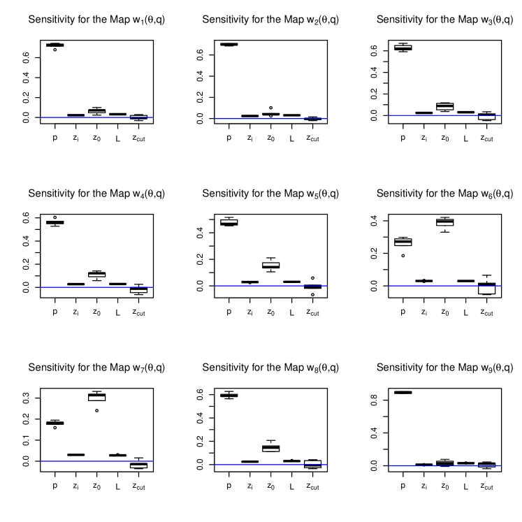
The sensitivity indices computed using the four different kernels are summarized in the boxplots shown in Figure 2. The size of each box represents the interquartile range (IQR). The upper bar attached to each box is at the value

$$\min\left\{\max(S),E_{3}+\frac{3}{2}IQR\right\},$$

and the lower bar is located at

$$\max\left\{\min(S),E_{1}-\frac{3}{2}IQR\right\},$$

where $S$ is the set of the four indices (corresponding to the four kernels) calculated for each $w_{i}$ for $i\in\{1,\ldots,9\}$, and $E_{1}$ and $E_{3}$ are the first and third quartiles of $S$ respectively boxplot .

From these results it is clear that the variability in output of each map $w_{i}$ is captured in large part by the two parameters $p$ and $z_{0}$. Although the sensitivity index for $L$ is relatively small, we still retain this parameter because it is known to be closely related to $z_{0}$ (seinfeld1998atmospheric, , Chap. 19). The remaining “unimportant” parameters, $z_{i}$ and $z_{\textit{cut}}$, may then be fixed at suitable constant values (we used $z_{i}=100$ and $z_{\textit{cut}}=2$, following hosseini2016airborne ). This reduces the dimensionality of the parameter space from $5$ to $3$ and allows us to redefine our parameter vector as

$$\boldsymbol{\theta}:=(p,z_{0},L).$$

We highlight that the negative values of the total Sobol index for $z_{\textit{cut}}$ appearing in Figure 2 are not physical but rather arise due to numerical errors in the Monte Carlo integration method used in the sensitivity package.

Figure 2: The Sobol total indices of the model parameters $\boldsymbol{\theta}$ for the maps $w_{i}$ defined in (22). Errors bars indicate variation between estimated value of Sobol total indices using different kernels.

We next identify the support of the prior distribution, which consists simply of the interval of allowable values for each unknown parameter. Every emission rate must be a non-negative number, so that

$$q_{j}\in[0,\infty),\qquad\text{for }j=1,2,3,4.$$

For the remaining parameters $p,z_{0},L$, we use the physically-motivated ranges listed in Table 1, which are slightly larger than the suggested ranges typically cited in the literature (see e.g., (seinfeld1998atmospheric, , Ch. 19)) to allow for more flexibility. Consequently, each map $w_{i}(\boldsymbol{\theta},\textbf{q})$ has a domain

$$\text{dom}(w_{i})=[0,0.6]\times[0,3]\times[-600,0]\times[0,\infty)^{4}.$$

With this information in hand, we are now in a position to create a space-filling design needed to construct the GP emulator as explained in Section 2. Due to computational budget constraints, we choose 64 points to construct our emulators. We display 2D projections of the corresponding maximin space-filling design for the three relevant parameters in Figure 3.

Table 1: Physically reasonable ranges for the parameters $p,z_{0},L$.

Parameter (units)	Symbol	Range
Velocity exponent	$p$	${[}0,0.6{]}$
Roughness length (m)	$z_{0}$	${[}0,3{]}$
Monin-Obukhov length (m)	$L$	${[}-600,0{]}$

Figure 3: Pairwise two-dimensional projections of the space-filling design with 64 points for emulating $\mathcal{A}$. Results were obtained by initializing the particle swarm algorithm using a LHD and iterating for 10,000 steps. The range of each parameter is normalized between $0$ and $1$ for easy visualization. The scatter plot in the second row depicts $z_{0}$ vs. $p$. The plots on the bottom row show $L$ vs. $p$ (left) and $L$ vs. $z_{0}$ (middle).

4.2 Construction and validation of the emulator

We now proceed as outlined in Section 2 to construct the emulator for maps $\mathfrak{a}_{ij}$ using GPs. The 64 different combinations of parameters $p,z_{0},L$ obtained from the space-filling design in the previous section are used to train the GP. To create the GPs for each of the 36 maps $\mathfrak{a}_{ij}(p,z_{0},L)$, we used the R package DiceKriging dupuy2015dicedesign . Unlike the sensitivity analysis in the previous sections where four different kernels were computed, the GPs here are constructed using only the isotropic squared exponential kernel.

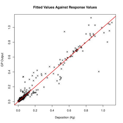
The DiceKriging package chooses a maximum likelihood estimate for the tuning parameters $r_{1},r_{2}$ for each map $\mathfrak{a}_{ij}$. To assess the quality of each emulator we perform a “leave one out” cross validation (LOOCV) (murphy2012machine, , Sec 1.4) on each of the nine sites $R_{1},R_{2},\ldots,R_{9}$ for the 64 design points shown in Figure 3; that is, we run the finite volume solver 64 times and save the predicted deposition value for each sites, yielding a total of $64\times 9$ points or predictions from the finite volume solver. For each point “left out” in the LOOCV, we plot in Figure 4 the deposition obtained from the finite volume solver versus the predicted value from the corresponding trained GP. This figure shows that the output of the GP is closely matched to the output of the finite volume solver at most design points, with the exception of a small number of outliers.

Figure 4: Comparison between deposition values predicted by the finite volume solver and the GP emulator using LOOCV for each of the $64\times 9$ data points obtained from the finite volume solver.

4.3 Source inversion

The GP emulator may now be employed to estimate the emission rates $q_{1},\ldots,q_{4}$, for the actual physical dataset which consists of dustfall jar measurements at the nine locations marked $R_{1},\ldots,R_{9}$ in Figure 1. Our first task is to specify the prior distribution for $\boldsymbol{\theta}$ and q. Following (11), we take the prior for $p,z_{0},L$ to be independent of the prior on q. Since we do not have any prior information about the values of the parameters $p,z_{0},L$ (other than an acceptable range), we choose a uniform distribution for each parameter

$$\mathbb{P}_{\textit{prior}}(p)\propto\mathbf{1}_{[0,0.6]}(p),\qquad\mathbb{P}_{\textit{prior}}(z_{0})\propto\mathbf{1}_{[0,3]}(z_{0}),\qquad\mathbb{P}_{\textit{prior}}(L)\propto\mathbf{1}_{[-600,0]}(L),$$

where $\mathbf{1}_{E}$ is the indicator function for the interval set $E$. For the source strengths q, we have the engineering estimates from previous independent studies shown in Table 2 which can be applied along with a non-negativity constraint to construct a suitable prior. In particular, we propose the following prior for source strengths based on a gamma distribution:

$$q_{j}\propto q_{j}^{\alpha_{j}-1}\exp(-\beta_{j}q_{j}).$$ (23)

The quantities $\alpha_{j}$ are called shape parameters, while the $\beta_{j}$ are rate parameters for the gamma distribution. Values for $\alpha_{j}$ and $\beta_{j}$ are derived from the engineering estimates $\textbf{q}=(q_{\textit{eng,j}})$ as the solution to the following system of equations:

$$\frac{\alpha_{j}-1}{\beta_{j}} =q_{\textit{eng,j}},$$

$$\mathit{qgamma}(0.99,\alpha_{j},\beta_{j}) =3q_{\textit{eng,j}}.$$

Here, $\mathit{qgamma}$ is the quantile function, which is just the inverse of the cumulative distribution function of the gamma density. Choosing $\alpha_{j}$ and $\beta_{j}$ in this way guarantees that the mode of the prior distribution for $q_{j}$ is located at the corresponding engineering estimate. Furthermore, $99\%$ of the prior mass is concentrated in the interval $(0,3q_{\textit{eng,j}})$ for each $q_{j}$ (gilchrist2000statistical, , Sec. 2.2).

Table 2: Engineering estimates of the source strengths from previous independent studies.

Source	Estimated emission rate [ton/yr]
$q_{\textit{eng},1}$	35
$q_{\textit{eng},2}$	80
$q_{\textit{eng},3}$	5
$q_{\textit{eng},4}$	5

Our next task is to specify the covariance matrix $\Sigma$ for the measurement noise in (9). Because the dustfall jars are well-separated, we assume that the measurement noise for each jar is independent from the others and hence take

$$\Sigma=\lambda I_{9\times 9},$$ (24)

where $\lambda>0$ is the variance of the measurement noise and $I_{9\times 9}$ is the $9\times 9$ identity matrix. The variance parameter $\lambda$ is related to the signal-to-noise ratio (SNR) of the measurements and can be estimated by minimizing the functional

$$J(\lambda)=\frac{1}{2}\int\left(\left\|\widehat{A}(p,L,z_{0})\textbf{q}-\textbf{w})\right\|_{2}+\left\|\textbf{q}-\textbf{q}_{\textit{eng}}\right\|_{2}\right)\,d\mathbb{P}_{\textit{post}}^{\lambda},$$ (25)

where $\textbf{q}_{\textit{eng}}=[35,80,5,5]^{T}\,{ton}/{yr}$, and the notation $\mathbb{P}_{\textit{post}}^{\lambda}$ is used to explicitly show the dependence of the posterior measure $\mathbb{P}_{\textit{post}}$ on the parameter $\lambda$. The motivation for defining $J(\lambda)$ in this way comes from the problem of choosing $\lambda$ to minimize the average value of the expression

$$(1-\delta)\left\|A(p,L,z_{0})\textbf{q}-\textbf{w})\right\|_{2}+\delta\left\|\textbf{q}-\textbf{q}_{\textit{eng}}\right\|_{2}\qquad\text{for }\delta\in[0,1].$$ (26)

Depending on the value of $\delta$, different weight can be given to the credibility of the atmospheric dispersion model compared to that of prior information about q. In particular, if $\delta=1$ then (26) reduces to $\left\|\textbf{q}-\textbf{q}_{\textit{eng}}\right\|_{2}$ and $\lambda$ is chosen to solely match the engineering estimates; on the other hand, taking $\delta=0$ leaves only the term $\left\|A(p,L,z_{0})\textbf{q}-\textbf{w})\right\|_{2}$ which chooses $\lambda$ solely based on minimizing the data misfit. We choose $\delta=\frac{1}{2}$, which is a compromise between the two extremes. After substituting into (26) and minimizing the expected value with respect to the posterior measure, the expression $J(\lambda)$ from (25) is easily obtained.

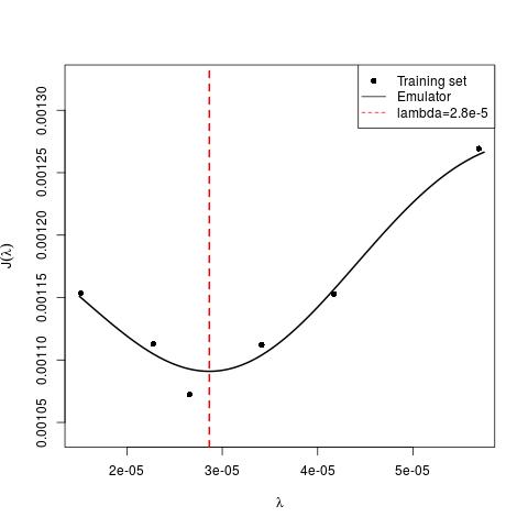
Computing $J(\lambda)$ analytically is not practically feasible and so we approximate it using a GP emulator, minimizing the emulator instead. To obtain design points for the GP, we evaluate $J$ for six different values of $\lambda$ using Markov Chain Monte Carlo integration, choosing only six points to keep the computational cost within reasonable limits. The design points were chosen empirically by identifying locations where the function $J$ changes the most, and the resulting simulation is shown in Figure 5. The minimum value of $J(\lambda)$ is attained at $\lambda\approx 2.8\times 10^{-5}$, which is the value of $\lambda$ we use in our source inversion framework for (24). Note that optimization with emulators is an emerging area of research for which a detailed background can be found in the paper osborne2009gaussian and references therein.

Figure 5: Emulator for $J(\lambda)$ in equation (25).

We now apply Algorithm 1 to generate samples from the posterior distribution, using the GP emulator $A(p,z_{0},L)$ to compute the likelihood ratio in Step 10 and parameter values listed in Table 3. When estimating integrals, we discard the first half of the samples (up to 500,000) and retain only every tenth iterate from there onward to reduce correlation between consecutive samples. Therefore, a total of 50,000 samples is used to approximate each integral with respect to the posterior.

Marginal posterior histograms are displayed in Figure 6, from which we observe that marginals for the emission rates $q_{j}$ are skewed and have well-defined modes. This is in line with our choice of a gamma prior, and the mode for these marginals is a reasonable point estimate for each $q_{j}$. To approximate the marginal mode we fit a gamma distribution to the histograms and take the point estimate to be the mode of the fitted distribution.

Table 3: Value of parameters used in Algorithm 1 for generating samples from the posterior distribution.

$N$	$\beta$	$\gamma_{1}$	$\gamma_{2}$	$\gamma_{3}$
$10^{6}$	$0.05$	$0.01$	$(2.38)^{2}$	$(0.1)^{2}$

The situation is slightly different for the parameters $p,z_{0},L$. The histogram for $p$ has no distinctive maximum point indicating that the data is not informative for this parameter. For $z_{0}$ and $L$, some values are more distinctive than others but the distinction is still not sharp. To choose a point estimate for these cases, we first fit a density over the histograms and then take the resulting mode as the point estimate, which is indicated in each case by a red dashed line in Figure 6.

Figure 6: Marginal posterior distribution for the three parameters $p,z_{0},L$ and the four emission rates $q_{1},\dots,q_{4}$.

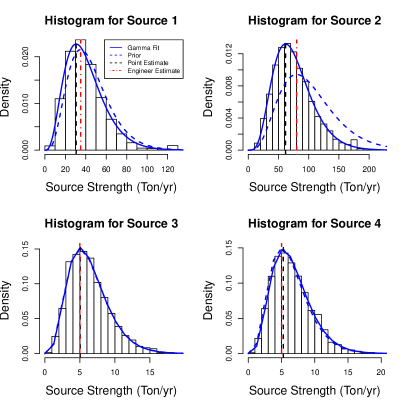
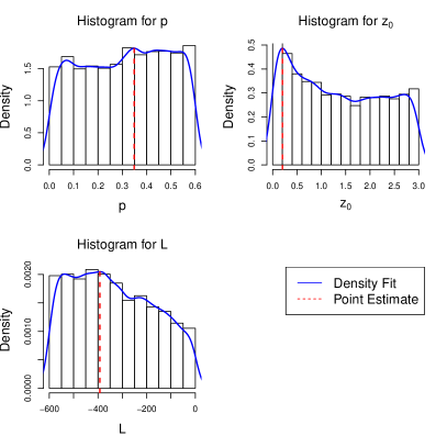
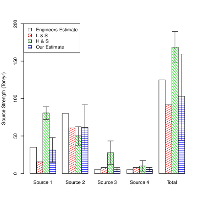
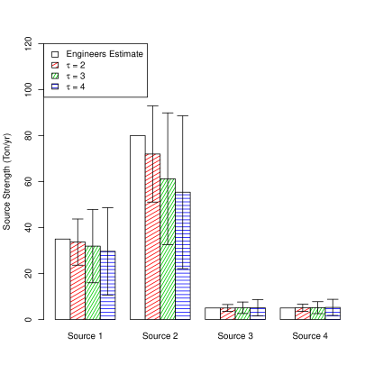
To quantify the uncertainty in each parameter, we employ a $68\%$ Bayesian confidence interval which is defined as follows: given a point estimate $x^{\ast}$ of a random variable $X$ distributed with probability density $\rho$, a $68\%$ Bayesian confidence interval is the radius of the ball centered at $x^{\ast}$ containing $68\%$ of the probability mass for $\rho$. The corresponding confidence interval is listed for each parameter in Table 4. The estimates of the $q_{j}$ are clearly more informative, which is due to the linearity of the forward map and stronger prior knowledge. The marginal modes and associated uncertainties for the $q_{j}$ are depicted graphically in Figure 7. These results suggest that the engineering estimates for sources $q_{1}$ and $q_{2}$ are most likely overestimates, whereas sources $q_{3}$ and $q_{4}$ are slightly underestimated. Furthermore, our estimates for sources $q_{2}$, $q_{3}$ and $q_{4}$ qualitatively agree with the results of previous studies in lushi2010inverse (L&S) and hosseini2016airborne (H&S).

The results in (L&S) were obtained using a Gaussian plume model and a least-squares based inversion method. Therefore, discrepancies between our estimates and those of (L&S) are expected given that we used a very different forward model. On the other hand, (H&S) used the same PDE based forward map as this study (although within a different Bayesian formulation) and so it is more informative to compare our results to those of (H&S). We note two key differences between our results. First of all, there is a notable difference between the estimates for $q_{1}$. In hosseini2016airborne , the parameters $p,z_{0},L$ are fixed at $0.2,0.05$ and $-10$, respectively. But these values depend strongly on environmental conditions, so a mis-assessment in the environmental conditions might lead to sub-optimal predictions. It was conjectured in hosseini2016airborne that this may be the underlying reason for the apparent overestimation of $q_{1}$ in comparison to previous studies. Furthermore, (H&S) obtained their estimates by marginalizing the posterior measure on $q_{j}$ only, whereas we marginalize the posterior measure on the $q_{j}$ and the model parameters $\boldsymbol{\theta}$. We believe that the discrepancy between our results and hosseini2016airborne highlights the importance of model calibration in atmospheric source inversion applications.

The second major difference is that our estimates have larger error bars in comparison to (H&S), although we note that our error bars are large enough to cover most previous estimates. This is largely due to differences in the parameter $\lambda$ which have a direct effect on posterior variance. We chose $\lambda$ by minimizing $J(\lambda)$ in (25) and achieved an SNR of $2.70$. This means that the strength of the signal is quite low compared to the noise of the measurements. In hosseini2016airborne , $\lambda$ is chosen to achieve an SNR of 10 which is why the error bars for those results are much smaller. Furthermore, our method accounts for uncertainties in the value of the model parameters $\boldsymbol{\theta}$ while these are fixed in the approach of (H&S).

We further observe that our estimate of the total emission is consistent with previous studies, with the exception of (H&S) which appears to have a higher estimate. This is mostly due to the over-estimation of $q_{1}$ which, as was mentioned before, is likely due to a lack of calibration in hosseini2016airborne . By allowing the model parameters to be calibrated automatically we have obtained estimates that are consistent with two previous studies that used very different methodologies, namely the engineering estimates and (L&S). This highlights the importance of model calibration in atmospheric source inversion studies. Furthermore, our uncertainty estimates are more realistic since we account for model parameter uncertainties and infer a better value of the signal-to-noise ratio. Although our uncertainty estimate for the total emission is relatively large in comparison to the estimate itself, this is due to the fact atmospheric source inversion problems are severely ill-posed and sensitive to model parameters.

Table 4: Parameters and their estimates and uncertainties.

Parameter	Point Estimate	$68\%$ Confidence Interval
$p$	0.3478	$[0.1498,0.5458]$
$z_{0}$	0.0811	$[0,1.5781]$
$L$	$-$379.45	$[-195.86,-563.04]$

Finally, we note that GP emulation is a crucial aspect of our inversion method that renders it cost-effective. The main computational bottleneck in our framework is the evaluations of the finite volume forward solver at the 64 design points used to construct the emulator. Given that the design points are independent not only of each other but also the measurements, these computations can be performed offline and in parallel. Every run of the finite volume code requires roughly two hours on a personal computer, while the emulator can be evaluated in a fraction of a second. Therefore, the cost of evaluating the emulator is negligible in comparison to the finite volume solver which enables us to perform Monte Carlo integration in a reasonable time. Clearly, such a calculation would be prohibitive had we employed the finite volume solver directly in the MCMC step.

In comparison to the previous approaches of hosseini2016airborne and lushi2010inverse our total computational cost (including the training of the emulator and design of experiment) is higher. For example, lushi2010inverse uses a Gaussian plume model which is much cheaper than the finite volume solver but comes at the cost of major simplifications to the physics. On the other hand, hosseini2016airborne uses a finite volume forward solver of the original PDEs, which is only evaluated four times. However, neither of these two approaches provides an automated calibration procedure, and so we claim that the extra computations in our methodology are a small price to pay for a richer solution structure with more realistic uncertainty estimates and rigorous model calibration.

Figure 7: Comparison between engineering estimates of the emission rates and our point estimates, along with the associated uncertainty. The “Total” column indicates the sum of emission rates from all four sources. Previous results from Lushi and Stockie lushi2010inverse (L&S) and Hosseini and Stockie hosseini2016airborne (H&S) are included for comparison purposes.

4.4 Effect of the prior choice

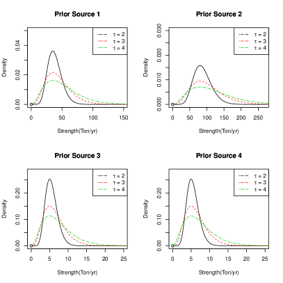
Here we study how the choice of the prior on emission rates affects the marginal posteriors. We use the same uniform priors on the model parameters $p,z_{0},L$ as before because those uniform priors are readily uninformative. We take the gamma priors of Section 4.3 and vary the parameters $\alpha_{j}$ and $\beta_{j}$ in (23). More precisely, we choose $\alpha_{j},\beta_{j}$ to solve

$$\frac{\alpha_{j}-1}{\beta_{j}} =q_{\textit{eng,j}},$$

$$\mathit{qgamma}(0.99,\alpha_{j},\beta_{j}) =\tau q_{\textit{eng,j}}.$$

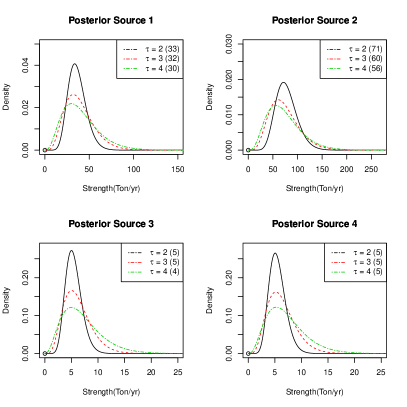
with $\tau=2,3,4$ and $qgamma$ being the quantile function for the Gamma distribution as before. Recall that these equations imply that all prior modes are centered at the engineering estimates but $\tau$ controls the spread of the priors. In fact, 99% of the prior mass lies in the interval $(0,\tau q_{\textit{eng},j})$. Then setting $\tau=2$ forces the prior to concentrate more tightly around the mode while $\tau=4$ corresponds to a flat prior. Figure 8 shows the three choices of the priors for each source as well as the corresponding marginal posteriors. For sources 1 and 2 a noticeable contraction of the posterior occurs, which is more noticeable for larger $\tau$. The contraction of the posterior implies that the data is in fact informative regarding the first two sources. On the other hand, the marginals on sources 3 and 4 are nearly identical to their priors, which is a sign that the data is not informative about these sources. We note that this observation is not surprising given the fact that the emissions from sources 3 and 4 are negligible in comparison to 1 and 2.

In Figure 9 we compare the pointwise estimators of the emission rates as well as uncertainty estimates for different choices of $\tau$. As expected, the uncertainties increase with $\tau$ since prior uncertainty directly affects posterior uncertainty. We also observe that smaller values of $\tau$ pull the pointwise estimates towards the engineering estimates, which is also in line with the intuition that choosing a prior that is too tight can result in the posterior being overwhelmed by the prior which tends to ignore the measured data. Furthermore, by comparing to Figure 8 we observe stronger posterior contraction relative to prior for the first two sources in the case where $\tau$ is larger. This indicates that the measurements are indeed informative in the direction of the larger sources. Relative contraction of the posterior appears to be weaker when $\tau=2$ indicating that the tighter prior is too strong.

Figure 8: Comparison between different choices of prior distribution on the emission rates and the corresponding posterior distributions for $\tau=2,3,4$. Smaller values of $\tau$ give tighter priors that are more concentrated around the engineering estimates while larger values result in more flat priors that are less informative.

Figure 9: Comparison between point estimates of emission rates using different prior distributions, along with the associated uncertainties.

4.5 Effect of emulator quality

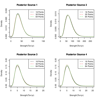
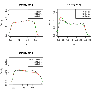
In this section we demonstrate how the quality of the GP emulator affects the posterior distributions in Figure 6. We construct a hierarchy of GP emulators using 16, 32 and 64 experimental designs and then solve the inverse problem with the corresponding emulators. Our results are summarized in Figure 10 where we plot the density fit to the posterior marginals of the model parameters and emission rates. We observe that the marginals on the emission rates have essentially converged and there is very little difference between the different emulators. More variations are present between the marginals on the model parameters $p,L$ and $z_{0}$. In the case of $p$ and $L$ the small perturbations are most likely due to numerical errors in computing the histograms and fitting the densities. In the case of $z_{0}$ we see larger variations, specifically in the maximal point emerging close to 0.25 which is present when 32 and 64 point experimental designs are utilized. The closeness of the 32 and 64 point density fits indicate convergence of the posterior marginals for $z_{0}$ and provide further confidence that the maximal point is indeed located near $0.25$.

Figure 10: Marginal posterior distributions of model parameters $p,L,z_{0}$ and the four emission rates $q_{1},\dots,q_{4}$, for different emulators using experimental designs with 16, 32 and 64 points.

5 Conclusions

We have developed a new method for simultaneously calibrating atmospheric dispersion models and solving source inversion problems. GP emulators are used to speed up the evaluation of the atmospheric dispersion model, which are then employed within a Bayesian framework to calibrate model parameters and estimate source strengths at the same time. This allows for automatic tuning of unknown model parameters rather than more heuristic approaches that are typically used in practice.

We demonstrated the effectiveness of our proposed method in an industrial case study concerning emissions of zinc from a lead-zinc smelter in Trail, BC, Canada. Our results agree with those of previous studies in the literature that are based on very different approaches. Hence, we conclude that the emulation process is an accurate and efficient one that has the added advantage of greatly speeding up the calculations by exploiting emulation.

Our proposed solution methodology is not restricted to atmospheric dispersion models governed by partial differential equations. Indeed, our method can be adapted to any application where one in dealing with a forward map that is linear in the primarily unknowns (such as the source strengths) but may depend nonlinearly on the model parameters.