The distribution of shortest path lengths in subcritical Erdős-Rényi networks

Abstract

Networks that are fragmented into small disconnected components are prevalent in a large variety of systems. These include the secure communication networks of commercial enterprises, government agencies and illicit organizations, as well as networks that suffered multiple failures, attacks or epidemics. The structural and statistical properties of such networks resemble those of subcritical random networks, which consist of finite components, whose sizes are non-extensive. Surprisingly, such networks do not exhibit the small-world property that is typical in supercritical random networks, where the mean distance between pairs of nodes scales logarithmically with the network size. Unlike supercritical networks whose structure has been studied extensively, subcritical networks have attracted relatively little attention. A special feature of these networks is that the statistical and geometric properties vary between different components and depend on their sizes and topologies. The overall statistics of the network can be obtained by a summation over all the components with suitable weights. We use a topological expansion to perform a systematic analysis of the degree distribution and the distribution of shortest path lengths (DSPL) on components of given sizes and topologies in subcritical Erdős-Rényi (ER) networks. From this expansion we obtain an exact analytical expression for the DSPL of the entire subcritical network, in the asymptotic limit. The DSPL, which accounts for all the pairs of nodes that reside on the same finite component (FC), is found to follow a geometric distribution of the form $P_{\rm FC}(L=\ell|L<\infty)=(1-c)c^{\ell-1}$, where $c<1$ is the mean degree. Using computer simulations we calculate the DSPL in subcritical ER networks of increasing sizes and confirm the convergence to this asymptotic result. We also obtain exact asymptotic results for the mean distance, $\langle L\rangle_{\rm FC}$, and for the standard deviation of the DSPL, $\sigma_{L,{\rm FC}}$, and show that the simulation results converge to these asymptotic results. Using the duality relations between subcritical and supercritical ER networks, we obtain the DSPL on the non-giant components of ER networks above the percolation transition.

I Introduction

Network models provide a useful framework for the analysis of a large variety of systems that consist of interacting objects Newman2010 ; Havlin2010 ; Estrada2011 . In these models, the objects are represented by nodes and the interactions between them are described by edges. A pair of nodes, $i$ and $j$, may be connected via many different paths. The shortest among these paths are of particular importance because they provide the fastest and often the strongest interaction. Broadly speaking, one can distinguish between two major classes of networks: supercritical networks, which are tightly connected, and subcritical networks, which are loosely connected. Supercritical networks form a giant component that encompasses a macroscopic fraction of all the nodes, while the typical distance between pairs of nodes on the giant component scales logarithmically with the network size. Examples of such networks are the world-wide-web, social networks, and infrastructure networks of transportation, telephone, internet and electricity. In contrast, subcritical networks are fragmented into small components that do not scale with the overall network size. Examples of fragmented networks include secure networks with controlled access, such as the communication networks of commercial enterprises, government agencies and illicit organizations Duijn2014 . Other examples include networks that suffered multiple failures, large scale attacks or epidemics, in which the remaining functional or uninfected nodes form small, isolated components Shao2008 ; Shao2009 . In spite of their prevalence, fragmented networks are of low visibility and have not attracted nearly as much attention as supercritical networks.

Random networks of the Erdős-Rényi (ER) type Erdos1959 ; Erdos1960 ; Erdos1961 are the simplest class of random networks and are used as a benchmark for the study of structure and dynamics in complex networks Bollobas2001 . The ER network ensemble is a maximum entropy ensemble, under the condition that the mean degree $\langle K\rangle=c$ is fixed. It is a special case of a broader class of random uncorrelated networks, referred to as configuration model networks Newman2001 ; Newman2010 ; Klein2012 . In an ER network of $N$ nodes, each pair of nodes is independently connected with probability $p$, such that the mean degree is $c=(N-1)p$. The ensemble of such networks is denoted by ER[$N,p$]. The degree distribution of these networks follows a Poisson distribution of the form

$$\pi(K=k)=\frac{e^{-c}c^{k}}{k!}.$$ (1)

ER networks exhibit a percolation transition at $c=1$ such that for $c>1$ there is a giant component, while for $0<c<1$ the network consists of small, isolated tree components Bollobas2001 ; Durrett2007 . The probability that a random node in the network resides on the giant component is denoted by $g=g(c)$. Clearly, below the percolation transition $g=0$. Above the transition Bollobas2001

$$g(c)=1+\frac{\mathcal{W}(-ce^{-c})}{c},$$ (2)

where $\mathcal{W}(x)$ is the Lambert $W$ function Olver2010 . For networks in the range $1<c<\ln N$, the probability $g$ satisfies $0<g<1$, namely the giant and finite components coexist, while for $c>\ln N$ the giant component encompasses the whole network and $g=1$.

To characterize the paths connecting random pairs of nodes, measures such as the mean distance and the diameter were studied Chung2002 ; Hofstad2005 ; Bollobas2007 ; Newman2001 ; Fronczak2004 ; Hartmann2017 . For supercritical ER networks, it was shown that the mean distance, $\langle L\rangle$, scales like $\langle L\rangle\sim\ln N/\ln c$, in agreement with rigorous results, showing that percolating random networks are small-world networks Chung2002 ; Bollobas2007 . For subcritical ER networks it was recently shown that the distribution of diameters over an ensemble of networks follows a Gumbel distribution of extreme values Hartmann2017 . This is due to the fact that in subcritical networks the diameter is obtained by maximizing the distances over all the small components. For supercritical networks, the entire distribution of shortest path lengths (DSPL) was calculated using various approximation techniques Dorogotsev2003 ; Blondel2007 ; Hofstad2007 ; Esker2008 ; Shao2008 ; Shao2009 ; Katzav2015 ; Nitzan2016 ; Melnik2016 . However, the DSPL of subcritical networks has not been studied.

The DSPL provides a natural platform for the study of dynamical processes on networks, such as diffusive processes, epidemic spreading, critical phenomena, synchronization, information propagation and communication Havlin2010 ; Newman2010 ; Estrada2011 ; Satorras2015 . Thermal and dynamical processes on networks resemble those of systems with long range interactions Bouchet2010 in the sense that extensivity is broken and standard statistical physics techniques do not apply. Therefore, it is important to develop theoretical approaches that take into account the topological and geometrical properties of complex networks. In fact, the DSPL provides exact solutions for various dynamical problems on networks. In the context of traffic flow on networks, the DSPL provides the distribution of transit times between all pairs of nodes, in the limit of low traffic load Barrat2008 . In the context of search processes, the DSPL determines the order in which nodes are explored in the breadth-first search protocol Barrat2008 . In the context of epidemic spreading, the DSPL captures the temporal evolution of the susceptible-infected epidemic, in the limit of high infection rate Satorras2015 . In the context of network attacks, the DSPL describes a generic class of violent local attacks, which spreads throughout the network Shao2015 . It is also used as a measure that quantifies the structural dissimilarities between different networks Schieber2017 .

The DSPL provides a useful characterization of empirical networks. For example, the DSPL of the protein network in Drosophila melanogaster was compared to the DSPL of a corresponding randomized network Giot2003 . It was shown that proteins in this network are significantly farther away from each other than in the randomized network, providing useful biological insight. In the context of brain research, it was found that the DSPL and the distribution of shortest cycle lengths Bonneau2017 determine the periods of oscillations in the activity of neural circuits Goldental2015 ; Goldental2017 . In essence, shortest paths and shortest cycles control the most important feedback mechanisms in these circuits, setting the characteristic time scales at which oscillations are sustained.

As mentioned above, in the asymptotic limit, $N\rightarrow\infty$, ER networks exhibit a percolation transition at $c=1$. For $c<1$, an ER network consists of finite components (FC), which are non-extensive in the network size, while for $c>1$ a giant component (GC) is formed, which includes a finite fraction of the nodes in the network Bollobas2001 . When two nodes, $i$ and $j$, reside on the same component, the distance, $\ell_{ij}$, between them is defined as the length of the shortest path that connects them. In the networks studied here, whose edges do not carry distance labels, the length of a path is given by the number of edges along the path. When $i$ and $j$ reside on different components, there is no path connecting them and we define the distance between them to be $\ell_{ij}\equiv\infty$. We denote the probability distribution $P_{\rm FC}(L=\ell)$ as the DSPL over all $\binom{N}{2}$ pairs of nodes in a subcritical ER network. The probability that two randomly selected nodes reside on the same component, and thus are at a finite distance from each other, is denoted by $P_{\rm FC}(L<\infty)=1-P_{\rm FC}(L=\infty)$.

Here we focus on the conditional DSPL between pairs of nodes that reside on the same component, denoted by $P_{\rm FC}(L=\ell|L<\infty)$, where $\ell=1,2,\dots,N-1$. The conditional DSPL satisfies

$$P_{\rm FC}(L=\ell|L<\infty)=\frac{P_{\rm FC}(L=\ell)}{P_{\rm FC}(L<\infty)}.$$ (3)

In this paper we use a topological expansion to perform a systematic analysis of the degree distribution and the DSPL on finite tree components of all sizes and topologies in subcritical ER networks. We find that in the asymptotic limit the DSPL is given by a geometric distribution of the form $P_{\rm FC}(L=\ell|L<\infty)=(1-c)c^{\ell-1}$, where $c<1$. Using computer simulations we calculate the DSPL in subcritical ER networks of increasing sizes and confirm the convergence to this asymptotic result. We also show that the mean distance between pairs of nodes that reside on the same component is given by $\langle L\rangle_{\rm FC}=1/(1-c)$. The average size of the tree components (obtained by random sampling of trees) is $\langle S\rangle_{\rm FC}=2/(2-c)$. However, the average tree component size, obtained by random sampling of nodes, is $\langle\widetilde{S}\rangle_{\rm FC}=1/(1-c)$. Thus, the mean distance turns out to scale linearly with the average tree component size on which a random node resides. This is in contrast to supercritical random networks, in which the mean distance scales logarithmically or even sub-logarithmically with the network size Chung2002 ; Hofstad2005 ; Bollobas2007 ; Cohen2003 . Using duality relations connecting the non-giant components of supercritical ER networks to the corresponding subcritical ER networks Bollobas2001 ; Molloy1995 ; Molloy1998 , we obtain the DSPL of the non-giant components of the ER network above the percolation transition.

The paper is organized as follows. In Sec. II we describe recent results for the DSPL of supercritical networks. In Sec. III we review some fundamental properties of subcritical ER networks, which are used in the analysis below. In Sec. IV we present the topological expansion. In Sec. V we apply the topological expansion to calculate the degree distribution of subcritical ER networks. In Sec. VI we calculate the mean and variance of the degree distribution. In Sec. VII we apply the topological expansion to calculate the DSPL of subcritical ER networks. In Sec. VIII we calculate the mean and variance of the DSPL. The results are discussed in Sec. IX and summarized in Sec. X. In Appendix A we present the calculation of the component size distribution, $P_{\rm FC}(S=s)$, in subcritical ER networks, which is used in the topological expansion. In Appendix B we present the calculation of the probability, $P_{\rm FC}(L<\infty)$, that two random nodes in a subcritical ER network reside on the same component.

II The DSPL of supercritical Erdős-Rényi networks

Consider a pair of random nodes, $i$ and $j$, in a supercritical ER network of $N$ nodes. The probability that both of them reside on the giant component is $g^{2}$. The probability that one of them resides on the giant component and the other resides on one of the finite components is $2g(1-g)$, while the probability that both reside on finite components is $(1-g)^{2}$. In case that both nodes reside on the giant component, they are connected to each other by at least one path. Therefore, the distance between them is finite. In case that one node resides on the giant component while the other node resides on one of the finite components, the distance between them is $\ell_{ij}=\infty$. In case that both nodes reside on finite components, a path between them exists only in the low probability case that they reside on the same component. The finite components are trees and therefore the shortest path between any pair of nodes is unique.

The DSPL of a supercritical ER network can be expressed by

$$P(L=\ell)=g^{2}P_{\rm GC}(L=\ell)+(1-g)^{2}P_{\rm FC}(L=\ell),$$ (4)

where the first term accounts for the DSPL between pairs of nodes that reside on the giant component and the second term accounts for pairs of nodes that reside on finite components. This form is particularly useful in the range of $1<c<\ln N$, in which the giant component and the finite components coexist. The probability that there is no path connecting a random pair of nodes is given by

$$P(L=\infty)=2g(1-g)+(1-g)^{2}P_{\rm FC}(L=\infty).$$ (5)

The first term in Eq. (5) accounts for the probability that one node resides on the giant component while the other resides on one of the finite components. The second term accounts for the probability that the two nodes reside on two different finite components and are thus not connected by a path. In order to obtain accurate results for the DSPL of an ER network in this regime, one needs to calculate both the DSPL of the giant component, $P_{\rm GC}(L=\ell)$, and the DSPL of the finite components, $P_{\rm FC}(L=\ell)=P_{\rm FC}(L=\ell|L<\infty)P_{\rm FC}(L<\infty)$. The giant component of an ER network with $1<c<\ln N$ is a more complicated geometrical object than the whole network. Its degree distribution deviates from the Poisson distribution and it exhibits degree-degree correlations. The degree distribution and degree-degree correlations in the giant component of supercritical ER networks with $1<c<\ln N$ were recently studied Tishby2018 . Using these results, the DSPL of the giant component was calculated Tishby2018 .

For $c>\ln N$ the network consists of a single connected component and the DSPL of the whole network can be calculated using the recursion equations presented in Refs. Katzav2015 ; Nitzan2016 . In this approach one denotes the conditional probability, $P(L>\ell|L>\ell-1)$, that the distance between a random pair of nodes, $i$ and $j$, is larger than $\ell$, under the condition that it is larger than $\ell-1$. A path of length $\ell$ from node $i$ to node $j$ can be decomposed into a single edge connecting node $i$ and node $r\in\partial_{i}$ (where $\partial_{i}$ is the set of all nodes directly connected to $i$), and a shorter path of length $\ell-1$ connecting $r$ and $j$. Thus, the existence of a path of length $\ell$ between nodes $i$ and $j$ can be ruled out if there is no path of length $\ell-1$ between any of the nodes $r\in\partial_{i}$, and $j$. For sufficiently large networks, the argument presented above translates into the recursion equation Nitzan2016

$$P(L>\ell|L>\ell-1)=G_{0}[P(L>\ell-1|L>\ell-2)],$$ (6)

where

$$G_{0}(x)=\sum_{k=0}^{\infty}x^{k}\pi(K=k),$$ (7)

is the generating function of the Poisson distribution. The case of $\ell=1$, used as the initial condition for the recursion equations is given by $P(L>1|L>0)=1-c/(N-1)$. The recursion equations provide a good approximation for the DSPL of supercritical ER networks Katzav2015 ; Nitzan2016 ; Melnik2016 , for values of $c$ that are sufficiently far above the percolation threshold. However, no exact result for the DSPL of supercritical ER networks is known. Interestingly, for random regular graphs, in which all the nodes are of the same degree, $k=c\geq 3$, there is an exact result for the DSPL, which can be expressed by a Gompertz distribution Gompertz1825 of the form Hofstad2005 ; Nitzan2016

$$P(L>\ell)=\exp\left[{-\beta(e^{b\ell}-1)}\right],$$ (8)

where $\beta=c/[N(c-2)]$ and $b=\ln(c-1)$. For a supercritical ER network with mean degree $c$, which is sufficiently far above the percolation threshold, the DSPL is qualitatively similar to the DSPL of a random regular graph with degree $\lfloor c+1/2\rfloor$. Here, $\lfloor x\rfloor$ is the integer part of $x$ and thus $\lfloor x+1/2\rfloor$ is the nearest integer to $x$. Unlike random regular graphs in which all the nodes are of the same degree, in supercritical ER networks, which follow the Poisson degree distribution, the shortest path length between a pair of nodes is correlated with the degrees of these nodes. The correlation is negative, namely nodes of high degrees tend to be closer to each other than nodes of low degrees. Another simplifying feature of random regular graphs with $c\geq 3$ is that the giant component encompasses the entire network ($g=1$) and thus all pairs of nodes are connected by finite paths. Since ER networks with $1<c<\ln N$ consist of a combination of a giant component and finite components, the DSPL exhibits a non-zero asymptotic tail and its calculation is more difficult.

The DSPL on the finite components in supercritical ER networks is a sub-leading term in the overall DSPL, which involves a fraction of $(1-g)^{2}P_{\rm FC}(L<\infty)$ from the $\binom{N}{2}$ pairs of nodes in the network. The factor of $(1-g)^{2}$ accounts for the fraction of pairs that reside on the finite components, while the fraction of those pairs that reside on the same component is given by $P_{\rm FC}(L<\infty)$. Except for the vicinity of the percolation transition, which occurs at $c=1$, this amounts to a small fraction of all pairs of nodes.

In the asymptotic limit, ER networks exhibit duality with respect to the percolation threshold. In a supercritical ER network of $N$ nodes the fraction of nodes that belong to the giant component is $g$ [Eq. (2)], while the fraction of nodes that belong to the finite components is $f=1-g$. Thus, the subcritical network that consists of the finite components is of size $N^{\prime}=Nf$. This network is an ER network whose mean degree is $c^{\prime}=cf$, where $c^{\prime}<1$. It means that the DSPL of the finite components of a supercritical ER network can be obtained from the analysis of its dual subcritical network Tishby2018 .

III Subcritical Erdős-Rényi networks

In the analysis presented below we use the fact that the components that appear in subcritical ER networks are almost surely trees, namely the expected number of cycles is non-extensive Bollobas2001 . In Appendix A we show that the expected number of tree components in a subcritical ER network of $N$ nodes is

$$N_{T}(c)=\left(1-\frac{c}{2}\right)N,$$ (9)

and the distribution of tree sizes is Bollobas2001 ; Durrett2007

$$P_{\rm FC}(S=s)=\frac{2s^{s-2}c^{s-1}e^{-cs}}{(2-c)s!}.$$ (10)

In these trees we define all the nodes of degree $k\geq 3$ as hubs and all the nodes of degree $k=1$ as leaves. Linear chains of nodes that have a hub on one side and a leaf on the other side are referred to as branches, while chains that have hubs on both sides are referred to as arms. In Fig. 1 we illustrate the structure of an ER network of size $N=100$ and $c=0.9$. It consists of 33 isolated nodes, 9 dimers, two chains of three nodes, two chains of four nodes, one tree with a single hub and four branches, one tree with two hubs and two larger trees of 10 and 14 nodes.

Figure 1: (Color online) Illustration of the structure of one instance of a subcritical ER network of $N=100$ nodes and $c=0.9$. It consists of 33 isolated nodes, 9 dimers, two chains of three nodes, two chains of four nodes, one tree with a single hub and four branches, one tree with two hubs and two larger trees of 10 and 14 nodes.

Selecting two random nodes in a subcritical ER network, the probability that they reside on the same component is denoted by $P_{\rm FC}(L<\infty)$. In Appendix B we show that

$$P_{\rm FC}(L<\infty)=\frac{c}{(1-c)N}.$$ (11)

Using this result and the fact that the first two terms of $P_{\rm FC}(L=\ell)$ are known exactly, namely $P_{\rm FC}(L=1)=p$ and $P_{\rm FC}(L=2)=(1-p)[1-(1-p^{2})^{N-2}]$ Katzav2015 , we obtain that $P_{\rm FC}(L=1|L<\infty)=1-c$ and $P_{\rm FC}(L=2|L<\infty)=c(1-c)$.

In the next Section we introduce the topological expansion method. In this approach, for each component size, $s$, we identify all the possible tree topologies supported by $s$ nodes, starting from the linear chain, which does not include any hubs, followed by single-hub topologies, double-hub topologies and higher order topologies, which include multiple-hubs. For each tree topology, we calculate its relative weight among all possible tree topologies of the same size. A special property of tree topologies is that each pair of nodes is connected by a single path. Therefore, in subcritical ER networks the shortest path between any pair of nodes is, in fact, the only path between them. Using this property we calculate the DSPL for each tree topology, and use the weights to obtain the DSPL over all the components that consist of up to $s$ nodes.

IV The topological expansion

Consider a tree that includes $h$ hubs. Embedded in this tree, there is a backbone tree, which consists only of the $h$ hubs and the $h-1$ arms that connect them. The structure of the backbone tree is described by its adjacency matrix, $A$. This is a symmetric $h\times h$ matrix, in which $A_{ij}=1$ if hubs $i$ and $j$ are connected by an arm, and $0$ otherwise. The degrees of the hubs in the backbone tree are denoted by the vector

$$\vec{a}=(a_{1},a_{2},\dots,a_{h}),$$ (12)

where

$$a_{i}=\sum_{j=1}^{h}A_{ij}.$$ (13)

The structure of the branches is described by the vector

$$\vec{b}=(b_{1},b_{2},\dots,b_{h}),$$ (14)

where $b_{i}$ is the number of branches connected to the $i^{\rm th}$ hub. The total number of branches in a tree is given by

$$b=\sum_{i=1}^{h}b_{i}.$$ (15)

The topology of a tree with $h$ hubs is fully described by the adjacency matrix, $A$, of its backbone tree and its branch vector $\vec{b}$. We denote such tree topology by

$$\tau=(h,A,\vec{b}).$$ (16)

In this classification, the linear chain structure is denoted by $\tau=(0,\cdot,2)$. It has no nodes and thus $h=0$. The matrix $A$ is not defined and replaced by the ”$\cdot$” sign. The linear chain has two leaf nodes and it is thus considered as a tree with two branches. A tree that includes a single hub with $b\geq 3$ branches is denoted by $\tau=(1,0,b)$. Here, the matrix $A=0$ is a scalar. A tree that includes two hubs with a branch vector $\vec{b}=(b_{1},b_{2})$, is denoted by $\tau=(2,A,\vec{b})$, where $A$ is a $2\times 2$ matrix of the form

$$A=\left(\begin{array}[]{cc}0&1\\ 1&0\end{array}\right).$$ (17)

A tree that consists of a chain of three hubs, with a branch vector $\vec{b}=(b_{1},b_{2},b_{3})$, is denoted by $\tau=(3,A,\vec{b})$, where $A$ is a $3\times 3$ matrix of the form

$$A=\left(\begin{array}[]{ccc}0&1&0\\ 1&0&1\\ 0&1&0\end{array}\right).$$ (18)

A tree that includes four hubs, consisting of one central hub surrounded by three peripheral hubs is denoted by $\tau=(4,A,\vec{b})$ where

$$A=\left(\begin{array}[]{cccc}0&1&1&1\\ 1&0&0&0\\ 1&0&0&0\\ 1&0&0&0\end{array}\right).$$ (19)

and $\vec{b}=(b_{1},b_{2},b_{3},b_{4})$.

In Fig. 2 we present all the possible topologies of the backbone tree that can be obtained with up to six hubs. The linear chain topology exists for all values of $h$. For $h\leq 3$ it is the only topology, while for $h\geq 4$ additional topologies appear and their number quickly increases. More specifically, for $h=1$ the backbone tree is a single hub, for $h=2$ it is a dimer and for $h=3$ it is a linear chain of three hubs. For $h=4$ there are two possible tree topologies: a linear chain of hubs and a tree that consists of a central hub surrounded by three peripheral hubs. For $h=5$ there are three possible topologies while for $h=6$ there are six possible topologies.

Figure 2: A list of all the possible backbone tree topologies that consist of up to six hubs ($h=1,2,\dots,6$). The linear chain topology appears for all values of $h$. For $h\leq 3$ it is the only topology, while for $h\geq 4$ more complex topologies appear and their number quickly increases.

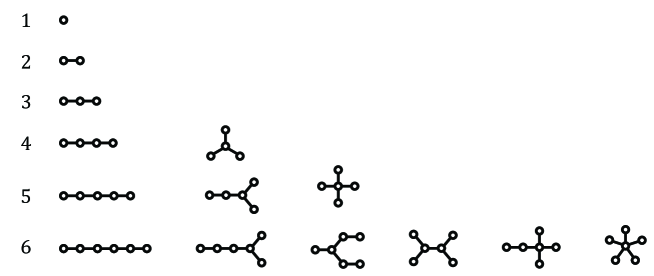
The topological expansion is performed such that the $s^{\rm th}$ order consists of all possible tree topologies that can be assembled from $s$ nodes. Since each branch consists of at least one node, the number of branches in a tree that consists of $s$ nodes and includes $h$ hubs must satisfy

$$b\leq s-h.$$ (20)

Unlike the branches, each arm may either consist of a single edge between the adjacent hubs or include one or more intermediate nodes. The number of arms connecting the $h$ hubs in the tree is $h-1$. The degree of each hub is given by the sum of the number of branches and the number of arms connected to it. While each branch is connected to only one hub, each arm is connected to two hubs, one on each side. Recalling that the degree of each hub is $k\geq 3$ we find that $2(h-1)+b\geq 3h$. Thus, the number of branches in a tree that includes $h$ hubs must satisfy

$$b\geq h+2.$$ (21)

Combining Eqs. (20) and (21) we obtain a condition on the minimal tree size that may include $h$ hubs. It takes the form

$$s\geq 2h+2.$$ (22)

We thus obtain a classification of all tree structures that can be assembled from $s$ nodes, where $s\geq 2$. For $s=2,3$ the linear chain is the only possible topology. Higher order topologies, which exist for $s\geq 4$, include at least one hub. In a tree of size $s\geq 4$, the number of hubs may take values in the range

$$h=1,2,\dots,\left\lfloor\frac{s}{2}-1\right\rfloor.$$ (23)

For each choice of $h$, the number of branches may take any value in the range

$$b=h+2,h+3,\dots,s-h.$$ (24)

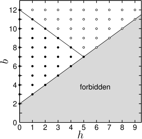
In Fig. 3 we illustrate the possible values of $b$ in a tree of $h$ hubs, which consists of $s$ nodes, given by Eq. (24), i.e., the range is bounded from below by $b=h+2$ and from above by $b=s-h$. Combinations of $(h,b)$ that are possible in a tree of $s=12$ nodes are marked by full circles, while combinations that exist only in larger trees are marked by empty circles.

Figure 3: Illustration of the range of possible values of $b$ (the number of branches) in a tree of $h$ hubs, which consists of $s$ nodes. This range is bounded from below by $b=h+2$, due to a topological constraint, regardless of $s$ (ascending straight line). For a network that consists of $s$ nodes, is is bounded from above by $b=s-h$ (descending straight line). The two lines intersect at $(h,2h+2)$. Combinations of $(h,b)$ that are possible in a tree of $s=12$ nodes are marked by full circles, while combination that exist only in larger trees are marked by empty circles. Each backbone tree can be represented by its adjacency matrix $A$, which is an $h\times h$ matrix. The topology of a complete tree is denoted by $\tau=(h,A,\vec{b})$, where $\vec{b}=(b_{1},\dots,b_{h})$ accounts for a specific division of the $b$ branches between the $h$ hubs.

The number of non-isomorphic tree topologies, $n(h)$, which can be assembled from $h$ nodes quickly increases as a function of $h$. For example, the values of $n(h)$ for $h=1,2,\dots,13$ are 1, 1, 1, 2, 3, 6, 11, 23, 47, 106, 235, 551 and 1301, respectively Steinbach1990 . An efficient algorithm for generating all the tree topologies that can be assembled from $h$ nodes, is presented in Refs. Wright1986 ; Beyer1980 . A list of all possible tree topologies up to $h=13$ is presented in Ref. Steinbach1990 . Other web resources include enumeration of such tree topologies up to $h=20$ Royle .

Each one of the possible topologies of the backbone tree is represented by its adjacency matrix, $A$, which is an $h\times h$ matrix. The degrees of the hubs in the backbone tree are given by $\vec{a}=(a_{1},a_{2},\dots,a_{h})$. Since the degrees of the hubs, which are given by $k_{i}=a_{i}+b_{i}$, must satisfy the condition $k_{i}\geq 3$, the components of the branch vector, $\vec{b}=(b_{1},b_{2},\dots,b_{h})$ satisfy the condition

$$b_{i}\geq(3-a_{i})\theta(3-a_{i}),$$ (25)

where $\theta(x)$ is the Heaviside function, which satisfies $\theta(x)=1$ for $x>0$ and $\theta(x)=0$ for $x\leq 0$. The number of branches required to satisfy this condition is $h+2$. In case that $b>h+2$, the remaining $b-h-2$ branches can be divided in many different ways between the $h$ hubs. The number of possible partitions of $x$ identical objects among $y$ distinguishable boxes is given by the multiset coefficient Stanley2011

$$\left(\binom{y}{x}\right)=\binom{x+y-1}{x}=\binom{x+y-1}{y-1}.$$ (26)

Therefore, the number of different tree topologies that can be obtained from a single topology of a backbone tree of $h$ hubs is

$$\left(\binom{h}{b-h-2}\right)=\binom{b-3}{h-1}.$$ (27)

Consider all the tree topologies that can be assembled from $s$ nodes. The weight of each tree topology, $\tau$, is given by the number of ways to distribute $s$ indistinguishable nodes among its branches and arms. We denote this weight by $W(\tau;s)$. In the case of a tree that consists of a linear chain of $s$ nodes, there are no degrees of freedom. Therefore, its weight is

$$W[\tau=(0,\cdot,2);s]=1.$$ (28)

The weight of a tree of $s$ nodes that consists of a single hub and $b$ branches is given by

$$W[\tau=(1,0,b);s]=\binom{s-2}{b-1}.$$ (29)

Here the binomial factor counts the number of possibilities to distribute $s-1$ nodes between the $b$ branches, such that each branch consists of at least one node. The weight of a tree with two hubs is

$$W[\tau=(2,A,\vec{b});s]=\binom{s-2}{b}.$$ (30)

In this case the binomial coefficient accounts for the number of ways to distribute $s-2$ nodes between the $b$ branches and one arm, where each branch includes at least one node.

In general, the weight of a tree structure consisting of $s$ nodes, $h$ hubs (connected by $h-1$ arms) and a branch vector $\vec{b}$ is

$$W[\tau=(h,A,\vec{b});s]=\binom{s-2}{h+b-2}.$$ (31)

This result can be understood as follows. Among the $s$ nodes, $h$ nodes are fixed as hubs while each one of the $b$ branches includes at least one node. Therefore, there are $x=s-h-b$ nodes that can be distributed among the $y=b+h-1$ branches and arms. Using Eq. (26) for the number of possible divisions of $x$ objects among $y$ boxes, one obtains the result of Eq. (31).

The contribution of each tree topology to the statistical properties of the network such as the degree distribution and the DSPL also depends on its symmetry. To account for the effect of the symmetry, we define the symmetry factor

$$X(\tau)=\frac{1}{|{\rm Aut}(\tau)|},$$ (32)

where ${\rm Aut}(\tau)$ is the automorphism group of $\tau$ Bollobas2001 , namely all the transformations that leave $\tau$ unchanged. It can be expressed as a product of the form

$$|{\rm Aut}(\tau)|=|{\rm Aut}(A)||{\rm Aut}(\vec{b})|,$$ (33)

where ${\rm Aut}(A)$ is the automorphism group of the backbone tree, which consists of the hubs alone, and ${\rm Aut}(\vec{b})$ is the automorphism group of the branches. While $|{\rm Aut}(A)|$ depends on the overall symmetry of the backbone tree, $|{\rm Aut}(\vec{b})|$ is given by

$$|{\rm Aut}(\vec{b})|=\prod_{i=1}^{h}b_{i}!.$$ (34)

For example, in the case of a linear chain of $s$ nodes,

$$X[\tau=(0,\cdot,2)]=\frac{1}{2}.$$ (35)

For a tree consisting of a single hub of $b$ branches

$$X[\tau=(1,0,b)]=\frac{1}{b!},$$ (36)

while for a tree that includes two hubs with $b_{1}$ and $b_{2}$ branches,

$$X[\tau=(2,A,\vec{b})]=\frac{1}{2b_{1}!b_{2}!}.$$ (37)

For a tree that consists of a central hub surrounded by three peripheral hubs

$$X[\tau=(4,A,\vec{b})]=\frac{1}{3b_{1}!b_{2}!b_{3}!b_{4}!}.$$ (38)

V The degree distribution

In this Section we show how to use the topological expansion to express the degree distribution $P_{\rm FC}(K=k)$ as a composition of the contributions of the different tree topologies. In this case the asymptotic form is known to be the Poisson distribution, $\pi(K=k)$, which enables us to validate the method.

Consider a tree that consists of $s\geq 2$ nodes, whose degree sequence is given by $k_{1},k_{2},\dots,k_{s}$. Since a tree of $s$ nodes includes $s-1$ edges, the sum of these degrees satisfies

$$\sum_{i=1}^{s}k_{i}=2(s-1).$$ (39)

We denote the number of nodes of degree $k$ by $N(K=k)$, where

$$\sum_{k=1}^{s-1}N(K=k)=s,$$ (40)

reflecting the fact that in a tree of size $s\geq 2$ the degrees of all nodes satisfy $k\geq 1$. In the special case of an isolated node, $s=1$ and $N(K=k)=\delta_{k,0}$, where $\delta_{k,k^{\prime}}$ is the Kronecker delta, which satisfies $\delta_{k,k^{\prime}}=1$ if $k=k^{\prime}$ and $\delta_{k,k^{\prime}}=0$ otherwise.

Eq. (39) can be written in the form

$$\sum_{k=1}^{s-1}kN(K=k)=2(s-1),$$ (41)

where $s\geq 2$. Combining Eqs. (40) and (41), we obtain

$$N(K=1)=2+\sum_{k=3}^{s-1}(k-2)N(K=k).$$ (42)

This result reflects the fact that any tree includes at least two leaf nodes and provides a relation between the degrees of the hubs and the number of leaf nodes in a tree. The number of nodes of degree $k=2$ can be obtained from

$$N(K=2)=s-N(K=1)-\sum_{k=3}^{s-1}N(K=k).$$ (43)

The topology of each tree structure can be described by $\tau=(h,A,\vec{b})$, where

$$h=\sum_{k=3}^{s-1}N(K=k)$$ (44)

is the number of hubs. The degrees of the hubs are given by

$$k_{1} = a_{1}+b_{1}$$

$$k_{2} = a_{2}+b_{2}$$

$$:$$

$$k_{h} = a_{h}+b_{h},$$ (45)

where $a_{i}$ is the number of arms and $b_{i}$ is the number of branches that are connected to hub $i$. The number of leaf nodes, with degree $k=1$ is given by $b=\sum_{i=1}^{h}b_{i}$. The remaining $s-h-b$ nodes are of degree $k=2$, namely

$$N(K=2)=s-h-b.$$ (46)

The number of nodes of degree $k$ in a linear chain of $s$ nodes is given by

$$N(K=k)=2\delta_{k,1}+(s-2)\delta_{k,2},$$ (47)

where $\delta_{k,k^{\prime}}$ is the Kronecker delta.

The number of nodes of degree $k$ in a tree that consists of $s$ nodes, and includes a single hub with $b$ branches, is

$$N(K=k)=b\delta_{k,1}+(s-1-b)\delta_{k,2}+\delta_{k,b}.$$ (48)

The number of nodes of degree $k$ in a tree that consists of $s$ nodes, and takes the form of a chain of $h$ hubs, with a total of $b$ branches distributed according to $\vec{b}=(b_{1},b_{2},\dots,b_{h})$, is

$$N(K=k)=b\delta_{k,1}+(s-h-b)\delta_{k,2}+\sum_{i=2}^{h-1}\delta_{k,b_{i}+2}+\delta_{k,b_{1}+1}+\delta_{k,b_{h}+1}.$$ (49)

Consider a tree of topology $\tau=(h,A,\vec{b})$ that consists of $s$ nodes. Such tree includes $h$ hubs, whose degrees in the backbone tree are given by $\vec{a}=(a_{1},a_{2},\dots,a_{h})$, and their branch vector is $\vec{b}=(b_{1},b_{2},\dots,b_{h})$. The number of nodes of degree $k$ is given by

$$N(K=k|\tau;s)=b\delta_{k,1}+(s-h-b)\delta_{k,2}+\sum_{i=1}^{h}\delta_{k,a_{i}+b_{i}}.$$ (50)

The degree distribution, $P_{\rm FC}(K=k|\tau;S=s)$, of trees of topology $\tau$, which consist of $s$ nodes, is given by

$$P_{\rm FC}(K=k|\tau;S=s)=\frac{N(K=k|\tau;s)}{s},$$ (51)

where $N(K=k|\tau;s)$ is given by Eq. (50). In the analysis below we use conditional degree distributions that are evaluated under different conditions. In Table 1 we summarize these distributions and list the equations from which they can be evaluated.

The degree distribution over all the tree topologies that consist of $s$ nodes is given by

$$P_{\rm FC}(K=k|S=s)=\frac{\sum\limits_{\{\tau|s\}}X(\tau)W(\tau;s)P_{\rm FC}(K=k|\tau;S=s)}{\sum\limits_{\{\tau|s\}}X(\tau)W(\tau;s)},$$ (52)

where $k=1,2,\dots,s-1$, the probabilities $P_{\rm FC}(K=k|\tau;S=s)$ are given by Eq. (51) and the summation is over all component topologies that can be constructed from $s$ nodes.

In Table 2 we present the conditional degree distributions $P_{\rm FC}(K=k|S=s)$ for trees of $s=2,3,\dots,10$ nodes. These distributions are determined by the combinatorial considerations presented above, after identifying by hand all the tree topologies that appear in trees of size $2\leq s\leq 10$. The probabilities are expressed in terms of constant rational numbers.

Summing up the degree distributions obtained from Eq. (52) over all the tree topologies that consist of $s^{\prime}=2,3,\dots,s$ nodes, with suitable weights, we obtain

$$P_{\rm FC}(K=k|2\leq S\leq s)=\frac{\sum\limits_{s^{\prime}=2}^{s}s^{\prime}P_{\rm FC}(S=s^{\prime})P_{\rm FC}(K=k|S=s^{\prime})}{\sum\limits_{s^{\prime}=2}^{s}s^{\prime}P_{\rm FC}(S=s^{\prime})}.$$ (53)

This equation provides an exact analytical expression for the degree distribution over all tree topologies up to any desired size, $s$ (not including the case of an isolated node). In Table 3 we present these expressions for $P_{\rm FC}(K=k|2\leq S\leq s)$ where $s=2,3,\dots,6$ and $k=1,2,\dots,5$. It turns out that in these expressions the dependence on the mean degree, $c$, always appears in terms of the parameter $\eta=\eta(c)$, which takes the form

$$\eta(c)=ce^{-c}.$$ (54)

The function $\eta(c)$ is a monotonically increasing function in the interval $0\leq c\leq 1$, where $\eta(0)=0$ and $\eta(1)=1/e$. Expanding the results of Eq. (53) in powers of the small parameter $c$, we obtain

$$P_{\rm FC}(K=k|2\leq S\leq s)=\frac{e^{-c}c^{k}}{(1-e^{-c})k!}\left(1+q_{s,k}c^{s-k}+\dots\right),$$ (55)

where $k=1,2,\dots,s-1$ and the coefficients $q_{s,k}$ are rational numbers of order $1$.

As $s$ is increased the degree distribution given by Eq. (55) converges to the asymptotic form given by

$$\pi_{\rm FC}(K=k)=\frac{e^{-c}c^{k}}{(1-e^{-c})k!},$$ (56)

which is the degree distribution of the whole subcritical ER network, except for the isolated nodes. Taking into account the isolated nodes, whose weight in the degree distribution is $\pi(K=0)=e^{-c}$, we obtain the Poisson distribution introduced in Eq. (1)

$$\pi(K=k)=e^{-c}\delta_{k,0}+(1-e^{-c})\pi_{\rm FC}(K=k)\theta(k),$$ (57)

where $\theta(k)$ is the Heaviside function.

This convergence to the Poisson degree distribution confirms the validity of the topological expansion and shows that the combinatorial factors were evaluated correctly. In Table 4 we present the leading correction terms, $q_{s,k}c^{s-k}$, of Eq. (55), obtained from the topological expansion, for all the tree structures that consist of up to $s$ nodes, where $s=2,3,\dots,10$. Tree structures with up to $s$ nodes support degrees in the range of $k=1,\dots,s-1$.

VI The mean and variance of the degree distribution

The moments of the degree distribution provide useful information about the network structure. The first and second moments are of particular importance. The first moment, $\langle K\rangle_{\rm FC}$ provides the mean degree. The width of the distribution is characterized by the variance, ${\rm Var}(K)=\langle K^{2}\rangle-\langle K\rangle^{2}$, where $\langle K^{2}\rangle$ is the second moment.

The $n^{\rm th}$ moment of the degree distribution, over all trees of topology $\tau$ that consist of $s$ nodes, can be expressed by

$${\mathbb{E}}[K^{n}|\tau;S=s]=\sum_{k=1}^{s-1}k^{n}P_{\rm FC}(K=k|\tau;S=s),$$ (58)

where $P_{\rm FC}(K=k|\tau;S=s)$ is given by Eq. (51). The $n^{\rm th}$ moment of the degree distribution over all tree topologies that consist of $s$ nodes is given by

$${\mathbb{E}}[K^{n}|S=s]=\frac{\sum\limits_{\{\tau|s\}}X(\tau)W(\tau;s){\mathbb{E}}[K^{n}|\tau;S=s]}{\sum\limits_{\{\tau|s\}}X(\tau)W(\tau;s)},$$ (59)

where ${\mathbb{E}}[K^{n}|\tau;S=s]$ is given by Eq. (58). For the special case of $n=1$, one obtains

$${\mathbb{E}}[K|S=s]=2-\frac{2}{s}.$$ (60)

This result represents a topological invariance and it applies to any tree of $s$ nodes, regardless of its topology, $\tau$. This is due to the fact that any tree of $s$ nodes includes $s-1$ edges and each edge is shared by two nodes. The results for the first two moments, ${\mathbb{E}}[K|S=s]$ and ${\mathbb{E}}[K^{2}|S=s]$, and for the variance ${\rm Var}[K|S=s]={\mathbb{E}}[K^{2}|S=s]-({\mathbb{E}}[K|S=s])^{2}$, for $s=2,3,\dots,10$ are shown in Table 2.

The $n^{\rm th}$ moment of the degree distribution over all trees that consist of up to $s$ nodes (except for the isolated nodes) is given by

$${\mathbb{E}}[K^{n}|2\leq S\leq s]=\frac{\sum\limits_{s^{\prime}=2}^{s}s^{\prime}P_{\rm FC}(S=s^{\prime}){\mathbb{E}}[K^{n}|S=s^{\prime}]}{\sum\limits_{s^{\prime}=2}^{s}s^{\prime}P_{\rm FC}(S=s^{\prime})},$$ (61)

where $P_{\rm FC}(S=s^{\prime})$ is given by Eq. (127). Performing the summation for a given value of $s$ provides an exact analytical expression for the $n^{\rm th}$ moment of the degree distribution over all tree topologies that consist of up to $s$ nodes. The resulting expressions for the mean degree, ${\mathbb{E}}[K|2\leq S\leq s]$, over all trees that consist of up to $s=2,3,\dots,6$ nodes, are presented in Table 3.

For a tree of size $s=1$, which consists of a single, isolated node, $P_{\rm FC}(S=1)=2e^{-c}/(2-c)$ and ${\mathbb{E}}[K^{n}|S=1]=0$. Thus in order to account for the isolated nodes, one should simply add the term $2e^{-c}/(2-c)$ to the denominator of Eq. (61).

In the limit of large $s$, the mean degree ${\mathbb{E}}[K|2\leq S\leq s]$ converges towards the asymptotic result, which is given by

$$\langle K\rangle_{\rm FC}=\frac{c}{1-e^{-c}}.$$ (62)

Taking into account the isolated nodes, we obtain

$$\langle K\rangle=(1-e^{-c})\langle K\rangle_{\rm FC}=c.$$ (63)

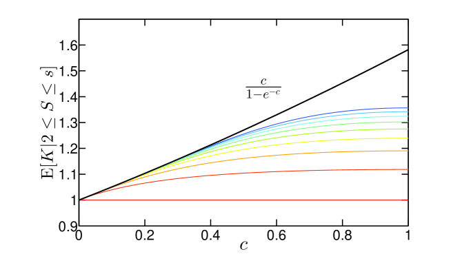
In Fig. 4 we present the mean degrees, ${\mathbb{E}}[K|2\leq S\leq s]$, as a function of $c$ (thin solid lines). The results are shown for all tree topologies of sizes smaller or equal to $s$, where $s=2,3,\dots,10$ (from bottom to top). The thick solid line shows the asymptotic result, $\langle K\rangle_{\rm FC}$, given by Eq. (62).

Figure 4: (Color online) Analytical results for the mean degree, ${\mathbb{E}}[K|2\leq S\leq s]$, over all tree topologies of sizes smaller or equal to $s$, as a function of $c$, for $s=2,3,\dots,10$ (solid lines), from bottom to top, respectively, obtained from Eq. (67). The thick solid line shows the asymptotic result, $\langle K\rangle_{\rm FC}$.

Below we derive closed form analytical expressions for the mean degree, ${\mathbb{E}}[K|2\leq S\leq s]$, over all tree topologies that consist of at least two nodes and up to $s$ nodes. Trees of size $s=1$, which consist of isolated nodes, are excluded from this summation because the degree of such nodes is $k=0$, while trees of size $s\geq 2$ do not include nodes of zero degree. Inserting the expression for ${\mathbb{E}}[K|S=s]$ from Eq. (60) into equation (61), with $n=1$, we obtain

$${\mathbb{E}}[K|2\leq S\leq s]=2-2\frac{\sum\limits_{s^{\prime}=2}^{s}P_{\rm FC}(S=s^{\prime})}{\sum\limits_{s^{\prime}=2}^{s}s^{\prime}P_{\rm FC}(S=s^{\prime})}.$$ (64)

This result can be expressed in the form

$${\mathbb{E}}[K|2\leq S\leq s]=2-\frac{2-c-2e^{-c}-2\sum\limits_{s^{\prime}=s+1}^{\infty}P_{\rm FC}(S=s^{\prime})}{1-e^{-c}-\sum\limits_{s^{\prime}=s+1}^{\infty}s^{\prime}P_{\rm FC}(S=s^{\prime})}.$$ (65)

Expressing the distribution $P_{\rm FC}(S=s^{\prime})$ by Eq. (127) we obtain

$${\mathbb{E}}[K|2\leq S\leq s]=2-\frac{\sqrt{2\pi}(2-c-2e^{-c})-c^{s}e^{-(c-1)(s+1)}\Phi\left(ce^{1-c},\frac{5}{2},s+1\right)}{\sqrt{2\pi}(1-e^{-c})-c^{s}e^{-(c-1)(s+1)}\Phi\left(ce^{1-c},\frac{3}{2},s+1\right)},$$ (66)

where $\Phi(z,s,a)$ is the Hurwitz Lerch $\Phi$ transcendent. An alternative approach for the evaluation of ${\mathbb{E}}[K|2\leq S\leq s]$ is to go back to Eq. (65) and replace the sums, $\sum\limits_{s^{\prime}=s+1}^{\infty}$ by integrals of the form $\int\limits_{s+1/2}^{\infty}$. Performing the integrations, we obtain

$${\mathbb{E}}[K|2\leq S\leq s]=2-\frac{\sqrt{2\pi}c(2-c-2e^{-c})-{(c-1-\ln c)^{3/2}}\Gamma\left[-\frac{3}{2},(c-1-\ln c)\left(s+\frac{1}{2}\right)\right]}{\sqrt{2\pi}c(1-e^{-c})-(c-1-\ln c)^{1/2}\Gamma\left[-\frac{1}{2},(c-1-\ln c)\left(s+\frac{1}{2}\right)\right]},$$ (67)

where $\Gamma(s,a)$ is the incomplete Gamma function. This function satisfies

$$\Gamma\left(-\frac{3}{2},x\right)=\frac{4}{3}\sqrt{\pi}\left[1-{\rm erf}(\sqrt{x})\right]+\frac{2e^{-x}(1-2x)}{3x^{3/2}},$$ (68)

and

$$\Gamma\left(-\frac{1}{2},x\right)=-2\sqrt{\pi}\left[1-{\rm erf}(\sqrt{x})\right]+\frac{2e^{-x}}{\sqrt{x}},$$ (69)

where ${\rm erf}(x)$ is the error function. In the limit of $c\rightarrow 0$ one can show that ${\mathbb{E}}[K|2\leq S\leq s]\rightarrow 1$.

For $c=1$ the $\Phi$ transcendent function in Eq. (66) can be replaced by the Hurwitz Zeta function. In this case

$${\mathbb{E}}[K|2\leq S\leq s]=2-\frac{\sqrt{2\pi}(2e-4)-4e\zeta\left(\frac{5}{2},s+1\right)}{\sqrt{2\pi}(e-1)-e\zeta\left(\frac{3}{2},s+1\right)},$$ (70)

where $\zeta(s,a)$ is the Hurwitz zeta function. In the limit of large $s$, one can approximate Eq. (70) by an asymptotic expansion of the form

$${\mathbb{E}}[K|2\leq S\leq s]=\frac{e}{e-1}-\sqrt{\frac{2}{\pi}}\frac{e(e-2)}{(e-1)^{2}}\frac{1}{\sqrt{s}}-\frac{2}{\pi}\frac{e^{2}(e-2)}{(e-1)^{3}}\frac{1}{s}+{\mathcal{O}}\left(\frac{1}{s^{3/2}}\right).$$ (71)

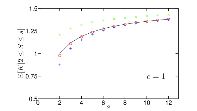
In Fig. 5 we present the mean degree ${\mathbb{E}}[K|2\leq S\leq s]$ over all trees of $S\leq s$ nodes, as a function of $s$ at the critical value of $c=1$. The analytical results (circles), obtained from Eq. (70), are in excellent agreement with the exact results of the asymptotic expansion (solid line). The only slight deviations are for $s=2$ and $3$, and they reflect the fact that Eq. (70) is based on the Stirling expansion, which becomes accurate for $s\geq 4$. The results of the asymptotic expansion to order $1/\sqrt{s}$ ($\times$), obtained from the first two terms of Eq. (71), exhibit large deviations from the exact results, particularly for small values of $s$. This means that next order correction should be taken into account, at least for such small values of $s$. Indeed, an expansion to order $1/s$ obtained by including the third term in Eq. (71), greatly improves the results ($+$).

Figure 5: (Color online) The mean degree ${\mathbb{E}}[K|2\leq S\leq s]$ over all trees of size smaller or equal to $s$, as a function of $s$ for $c=1$. The analytical results (circles), obtained from Eq. (70), are in excellent agreement with the exact results of the asymptotic expansion (solid line). The results of the asymptotic expansion to order $1/\sqrt{s}$ ($\times$), obtained from the first two terms of Eq. (71), exhibit large deviations from the exact results, particularly for small values of $s$. However, an expansion to order $1/s$ obtained by including the third term in Eq. (71), greatly improves the results ($+$).

Using Eq. (61) one can obtain exact analytical expressions for the second moment of the degree distribution over all trees of size $2\leq S\leq s$. The results for small trees, which consist of up to $s=2,3,\dots,6$ nodes, are shown in Table 3. In the limit of large $s$, the second moment ${\mathbb{E}}[K^{2}|2\leq S\leq s]$ converges towards the asymptotic result, which is given by

$$\langle K^{2}\rangle_{\rm FC}=\frac{c(c+1)}{1-e^{-c}}.$$ (72)

Taking into account the isolated nodes, we obtain

$$\langle K^{2}\rangle=(1-e^{-c})\langle K^{2}\rangle_{\rm FC}=c(c+1).$$ (73)

The variance of the degree distribution over all trees that consist of up to $s$ nodes is given by

$${\rm Var}[K|2\leq S\leq s]={\mathbb{E}}[K^{2}|2\leq S\leq s]-({\mathbb{E}}[K|2\leq S\leq s])^{2}.$$ (74)

Using the results presented in Table 3 for the first and second moments of the degree distributions over small trees of sizes $s=2,3,\dots,5$, we obtain

$${\rm Var}[K|2\leq S\leq 2] = 0$$

$${\rm Var}[K|2\leq S\leq 3] = \frac{2\eta+2\eta^{2}}{(2+3\eta)^{2}}$$

$${\rm Var}[K|2\leq S\leq 4] = \frac{18\eta+78\eta^{2}+90\eta^{3}+96\eta^{4}}{\left(6+9\eta+16\eta^{2}\right)^{2}}$$

$${\rm Var}[K|2\leq S\leq 5] = \frac{288\eta+1248\eta^{2}+3960\eta^{3}+5016\eta^{4}+6920\eta^{5}+7500\eta^{6}}{\left(24+36\eta++64\eta^{2}+125\eta^{3}\right)^{2}}.$$ (75)

In the limit of large $s$, the variance ${\rm Var}[K|2\leq S\leq s]$ converges towards the asymptotic result, $\sigma^{2}_{K,{\rm FC}}={\rm Var}(K)$, where $\sigma_{k,{\rm FC}}$ is the standard deviation of the degree distribution over all the finite components. The asymptotic variance is given by

$$\sigma^{2}_{K,{\rm FC}}={\rm Var}(K)=\frac{c}{1-e^{-c}}-\frac{c^{2}e^{-c}}{(1-e^{-c})^{2}}.$$ (76)

Taking into account the isolated nodes, we obtain

$$\sigma^{2}_{K}=\langle K^{2}\rangle-(\langle K\rangle)^{2}=c.$$ (77)

VII The distribution of shortest path lengths

In this Section we apply the topological expansion to obtain the DSPL of subcritical ER networks and to express it in terms of the contributions of the different tree topologies. Summing up the contributions for all possible tree topologies supported by up to $s$ nodes, we express the DSPL as a power series in $c$, and find its asymptotic form in the limit of $N\rightarrow\infty$.

For each value of $s=2,3,\dots$, we identify all the tree topologies, $\tau$, supported by $s$ nodes. For each one of these tree topologies, and for $\ell=1,2,\dots,s-1$, we calculate the number, $N(L=\ell|\tau;s)$ of pairs of nodes that reside at a distance $\ell$ from each other. We then sum up these contributions over all the possible ways to assemble $s$ nodes into the given tree topology. Below we describe the enumeration of the shortest paths for a few simple examples of tree topologies.

In a linear chain of $s$ nodes there are $s-\ell$ pairs of nodes at distance $\ell$ from each other. Therefore,

$$N[L=\ell|\tau=(0,\cdot,2);s]=\binom{s-\ell}{1}$$ (78)

A convenient way to evaluate the number of such pairs is to take a pair of nodes at a distance $\ell$ from each other and reduce the chain of $\ell+1$ nodes between them into a single node, which is marked in order to distinguish it from the other nodes. This results in a reduced network of $k-\ell$ nodes, one of which is the marked node. At this point, counting the number of pairs of nodes that are at a distance $\ell$ from each other is equivalent to counting the number of different locations of the marked node in the reduced network. In Fig. 6 we illustrate this procedure for the case of a linear chain of nodes. Since each node in the reduced chain may be the marked node, one concludes that in the original chain there are $s-\ell$ pairs of nodes at a distance $\ell$ from each other.

Figure 6: (Color online) Illustration of the collapse process that is used in order to obtain the combinatorial factors for the DSPL on a finite component. In this case, the number of pairs of nodes that are at a distance of $\ell=3$ from each other on a linear chain of size $s=9$ (top chain) is equal to the number of possible locations of the marked node (large empty circle) on the reduced chain of $s-\ell=6$ nodes (bottom chain).

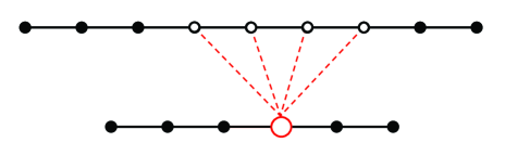
For a tree of $s$ nodes that includes a single hub and $b$ branches, the number of pairs of nodes at a distance $\ell$ from each other is

$$N[L=\ell|\tau=(1,0,b),s]=b\binom{s-\ell}{b}+(\ell-1)\binom{b}{2}\binom{s-\ell}{b-1}.$$ (79)

In this case there are many different configurations due to the different ways to distribute the nodes between the $b$ branches. Therefore, we need to sum up the numbers of pairs of nodes at distance $L=\ell$ from each other in all the different configurations. In this calculation we distinguish between pairs of nodes that reside on the same branch and pairs of nodes that reside on different branches. To calculate the number of pairs of nodes residing on the same branch and are at a distance $L=\ell$ apart, we pick one such pair of nodes and reduce the chain of $\ell+1$ nodes between them into a single node. This node is marked in order to keep track of its location. The reduced network now consists of $s-\ell$ nodes. We then evaluate the number of ways to distribute these $s-\ell$ nodes between the $b$ branches and the number of ways to place the marked node in its own branch. Essentially, the marked node splits its branch into two parts. This means that the number of possible configurations is equal to the number of possible ways to distribute $s-\ell$ nodes to $b+1$ urns. The first binomial coefficient in Eq. (79) accounts for the number of such distributions.

To calculate the number of pairs of nodes that reside on different branches and are at a distance $\ell$ apart from each other, we first arrange all $s$ nodes in a linear chain. We choose a pair of nodes that are at a distance $\ell$ from each other and reduce the $\ell+1$ nodes between them into a single node. This results in a reduced chain of $s-\ell$ nodes, one of which is the marked node. We proceed in two stages. In the first stage we consider the two branches on which the nodes $i$ and $j$ reside as a single branch, which now includes the marked node. The binomial coefficient $\binom{s-\ell}{b-1}$ accounts for the number of ways to distribute the nodes into $b-1$ urns and to choose randomly the location of the marked node. In the second stage we randomly choose the location of the hub among the $\ell-1$ nodes between $i$ and $j$ and connect all the end-points of all other $b-2$ branches to this node. Apart from this, there are $\binom{b}{2}$ possible ways to choose the branches on which $i$ and $j$ are located.

The approach presented above can also be used to evaluate the number of pairs of nodes at a distance $L=\ell$ apart that reside on branches that do not share a hub. In this case one needs to account for the number of possible ways to locate two or more hubs along the segment of $\ell-1$ nodes between $i$ and $j$. For a tree of $s$ nodes, which includes two hubs, we obtain

$$N[L = \ell|\tau=(2,A,\vec{b});s]=(b_{1}+b_{2}+1)\binom{s-\ell}{b_{1}+b_{2}+1}$$ (80)

$$+ (\ell-1)\left[{\binom{b_{1}+1}{2}}+{\binom{b_{2}+1}{2}}\right]{\binom{s-\ell}{b_{1}+b_{2}}}$$

$$+ b_{1}b_{2}{\binom{\ell-1}{2}}{\binom{s-\ell}{b_{1}+b_{2}-1}},$$

where $A$ is given by Eq. (17) and $\vec{b}=(b_{1},b_{2})$. Generalizing this result to the case of a linear chain of $h$ hubs we obtain

$$N[L = \ell|\tau=(h,A,\vec{b}),s]=(b+h-1)\binom{\ell-1}{0}\binom{s-\ell}{b+h-1}$$ (81)

$$+ \left[\binom{b_{1}+1}{2}+\sum_{i=2}^{h-1}\binom{b_{i}+2}{2}+\binom{b_{h}+1}{2}\right]\binom{\ell-1}{1}\binom{k-\ell}{b+h-2}$$

$$+ \sum_{r=2}^{h-1}\left[b_{1}(b_{r+1}+1)+\sum_{i=1}^{h-r-1}(b_{i}+1)(b_{i+r}+1)+(b_{h-r}+1)b_{h}\right]$$

$$\times \binom{\ell-1}{r}\binom{s-\ell}{b+h-r-1}+b_{1}b_{h}\binom{\ell-1}{h}\binom{s-\ell}{b-1},$$

where $A$ is an $h\times h$ Toeplitz matrix that satisfies $A_{ij}=1$ if $j=i\pm 1$ and $A_{ij}=0$ otherwise. Similarly, for a tree that consists of a central hub, which is surrounded by $h-1$ peripheral hubs, $N(L=\ell|\tau;s)$ is given by

$$N[L = \ell|\tau=(h,A,\vec{b});s]=(b+h-1)\binom{\ell-1}{0}\binom{s-\ell}{b+h-1}$$ (82)

$$+ \left[\binom{b_{1}+h-1}{2}+\sum_{i=2}^{h}\binom{b_{i}+1}{2}\right]\binom{\ell-1}{1}\binom{s-\ell}{b+h-2}$$

$$+ (b_{1}+h-2)\sum_{i=2}^{h}b_{i}\binom{\ell-1}{2}\binom{s-\ell}{b+h-3}$$

$$+ \sum_{i=2}^{h}\sum_{j=i+1}^{h}b_{i}b_{j}\binom{\ell-1}{3}\binom{s-\ell}{b+h-4},$$

where $A_{1j}=1$ for $j\geq 2$, $A_{i1}=1$ for $i\geq 2$ and $A_{ij}=0$ otherwise.

We will now derive an equation for the number of pairs of nodes at a distance $\ell$ from each other in any given tree of $s$ nodes, whose structure is given by the topology $\tau=(h,A,\vec{b})$. Such tree includes $h$ hubs, whose degrees are given by the vector

$$\vec{k}=(k_{1},k_{2},\dots,k_{h}),$$ (83)

where $k_{i}=a_{i}+b_{i}$. For convenience we also define the vector

$$\vec{k}^{\prime}=(k_{1}-1,k_{2}-1,\dots,k_{h}-1).$$ (84)

The hubs form a backbone tree of $h$ nodes, described by the adjacency matrix, $A$, of dimensions $h\times h$. For any pair of hubs, $i$ and $j$, which are connected by an arm (regardless of its length in the complete tree), the matrix element $A_{ij}=1$, while otherwise $A_{ij}=0$. From the adjacency matrix, $A$, one can obtain the $h\times h$ distance matrix, $D$, of the backbone tree, which consists of the hubs alone. This is a symmetric matrix, whose matrix element $D_{ij}$ is the distance between hub $i$ and hub $j$ on the backbone tree, and the diagonal elements are $D_{ii}=0$. For the analysis presented below, it is useful to express the distance matrix as a sum of symmetric binary matrices in the form

$$D=D_{\bf 1}+2D_{\bf 2}+3D_{\bf 3}+\dots+(h-1)D_{h-1},$$ (85)

where $(D_{\ell})_{ij}=1$ if $D_{ij}=\ell$ and $(D_{\ell})_{ij}=0$ otherwise. The matrix $D_{\ell}$, $\ell=1,2,\dots,h-1$ is called the $\ell^{\rm th}$ order vertex-adjacency matrix Janezic2015 . It can be obtained directly from the adjacency matrix, $A$, by constructing its powers $A^{1}$, $A^{2}$, $\dots$, $A^{\ell}$. In case that $(A^{\ell})_{ij}\geq 1$, under the condition that $(A^{\ell^{\prime}})_{ij}=0$ for all the lower powers of $A$, namely $\ell^{\prime}=1,2,\dots,\ell-1$, then $(D_{\ell})_{ij}=1$, and otherwise $(D_{\ell})_{ij}=0$.

Each pair of nodes, $i$ and $j$ in the network can be classified according to the number of hubs, $\nu_{ij}$, along the path between them. If $i$ and $j$ reside on the same branch or on the same arm, $\nu_{ij}=0$. If they reside on different branches or arms that emanate from the same hub, $\nu_{ij}=1$. In case that $i$ and $j$ reside on branches or arms that do not share a hub, we denote by $h_{i}$ the hub that is nearest to $i$ along the path to $j$ and by $h_{j}$ the hub that is nearest to $j$ along the path to $i$. We denote by $D_{ij}$ the distance between the hubs $h_{i}$ and $h_{j}$ on the backbone tree, which consists of the hubs alone. The number of hubs along the shortest path between nodes $i$ and $j$ can be expressed by $\nu_{ij}=D_{ij}+1$. Thus, $\nu_{ij}$ may take values in the range $0\leq\nu_{ij}\leq h$.

The number of pairs of nodes that are at a distance $\ell$ from each other can be expressed in the form

$$N(L=\ell|\tau,s)=\sum_{\nu=0}^{h}N_{\nu}(L=\ell|\tau,s),$$ (86)

where $N_{\nu}(L=\ell|\tau,s)$ is the number of pairs of nodes, $i$ and $j$ that are at a distance $\ell$ from each other, and along the path between them there are $\nu$ hubs.

For pairs of nodes that reside on the same branch or on the same arm, for which $\nu=0$, we obtain

$$N_{0}(L=\ell|\tau,s)=(b+h+1)\binom{\ell-1}{0}\binom{s-\ell}{b+h-1}.$$ (87)

For pairs of nodes that reside on different branches or arms that emanate from the same hub, for which $\nu=1$, we obtain

$$N_{1}(L=\ell|\tau,s)=\binom{\ell-1}{1}\binom{s-\ell}{b+h-2}\sum_{i=1}^{h}\binom{k_{i}}{2}.$$ (88)

For pairs of nodes for which $\nu\geq 2$ we obtain

$$N_{\nu}(L=\ell|\tau,s)=\frac{1}{2}\binom{\ell-1}{\nu}\binom{s-\ell}{b+h-\nu-1}\sum_{i=1}^{h}\sum_{j=1}^{h}k^{\prime}_{i}k^{\prime}_{j}\delta_{D_{ij},\nu-1}.$$ (89)

Eq. (89) can be written in the form

$$N_{\nu}(L=\ell|\tau,s)=\frac{1}{2}\binom{\ell-1}{\nu}\binom{s-\ell}{b+h-\nu-1}\vec{k}^{\prime T}D_{\nu-1}\vec{k}^{\prime},$$ (90)

where $\vec{k}^{\prime T}$ is the transpose of $\vec{k}^{\prime}$.

The distribution $P_{\rm FC}(L=\ell|\tau;L<\infty,S=s)$, for trees of a given topology, $\tau$, assembled from $s$ nodes, is given by

$$P_{\rm FC}(L=\ell|\tau;L<\infty,S=s)=\frac{N(L=\ell|\tau;s)}{{\binom{s}{2}}W(\tau;s)}.$$ (91)

In the analysis below we use different types of DSPLs. In Table 1 we summarize these distributions and list the equations from which each one of them can be evaluated.

The DSPL over components of all topologies that consist of $s$ nodes, is given by

$$P_{\rm FC}(L=\ell|L<\infty,S=s)=\frac{\sum\limits_{\{\tau|s\}}X(\tau)W(\tau;s)P_{\rm FC}(L=\ell|\tau;L<\infty,S=s)}{\sum\limits_{\{\tau|s\}}X(\tau)W(\tau;s)},$$ (92)

where the summation is over all component topologies which can be constructed from $s$ nodes, In Table 5 we present the probabilities $P_{\rm FC}(L=\ell|L<\infty,S=s)$ for trees of $s=2,3,\dots,10$ nodes. These probabilities are determined by combinatorial considerations and are expressed in terms of constant rational numbers.

To obtain the DSPL over all the components of sizes $s^{\prime}\leq s$, we sum up the results of Eq. (92) over all these components:

$$P_{\rm FC}(L=\ell|L<\infty,S\leq s)=\frac{\sum\limits_{s^{\prime}=2}^{s}\binom{s^{\prime}}{2}P_{\rm FC}(S=s^{\prime})P_{\rm FC}(L=\ell|L<\infty,S=s^{\prime})}{\sum\limits_{s^{\prime}=2}^{s}\binom{s^{\prime}}{2}P_{\rm FC}(S=s^{\prime})}.$$ (93)

This equation provides an exact analytical expression for the degree distribution over all tree topologies up to any desired size, $s$. In Table 6 we present these expressions for $P_{\rm FC}(L=\ell|L<\infty,S\leq s)$ where $s=2,3,\dots,6$ and $\ell=1,2,\dots,5$. It turns out that in these expressions the mean degree, $c$, always appears in the form $\eta(c)=ce^{-c}$, which is defined in Eq. (54).

Expanding the results of Eq. (93) as a power series in the small parameter $c$, we find that

$$P_{\rm FC}(L=\ell|L<\infty,S\leq s)=(1-c)c^{\ell-1}\left(1+r_{s,\ell}c^{s-\ell}+\dots\right),$$ (94)

where $\ell=2,3,\dots,s-1$ and the coefficient $r_{s,\ell}$ is a rational number of order $1$. In Table 7 we present the leading finite size correction terms, $r_{s,\ell}c^{s-\ell}$, of Eq. (94), obtained from the topological expansion, for all the tree structures that consist of up to $s$ nodes, where $s=2,3,\dots,10$. Tree structures with up to $s$ nodes support distances in the range of $\ell=1,\dots,s-1$. In the limit of large $s$, these results converge towards the asymptotic form

$$P_{\rm FC}(L=\ell|L<\infty)=(1-c)c^{\ell-1},$$ (95)

which turns out to be the DSPL of the entire subcritical network in the asymptotic limit of $N\rightarrow\infty$. In spite of its apparent simplicity, this is a surprising and nontrivial result, which was not anticipated when we embarked on the topological expansion. Eq. (95) is essentially a mean field result. Normally, a mean field result for the DSPL is expected to represent the shell structure around a typical node. However, in this case there is no typical node. The shell structures around each node strongly depends on the size and topology of the component on which it resides as well as on its location in the component. Only by combining the contributions of all pairs of nodes one obtains the simple expression of Eq. (95).

The DSPL given by Eq. (95) is a conditional distribution, under the condition that the selected pair of nodes reside on the same component. In fact, it is a subleading component of the overall DSPL of the network, because in subcritical networks most pairs of nodes reside on different components, and are thus at an infinite distance from each other. The overall DSPL can be expressed by

$$P_{\rm FC}(L=\ell)=P_{\rm FC}(L<\infty)P_{\rm FC}(L=\ell|L<\infty),$$ (96)

where $P_{\rm FC}(L<\infty)$ is given by Eq. (11). Therefore,

$$P_{\rm FC}(L=\ell)=\frac{c^{\ell}}{N}$$ (97)

for $\ell=1,2,\dots,N-1$, and

$$P_{\rm FC}(L=\infty)=1-\frac{c}{(1-c)N}.$$ (98)

The tail distribution that corresponds to the probability distribution function of Eq. (95) is given by

$$P_{\rm FC}(L>\ell|L<\infty)=c^{\ell}.$$ (99)

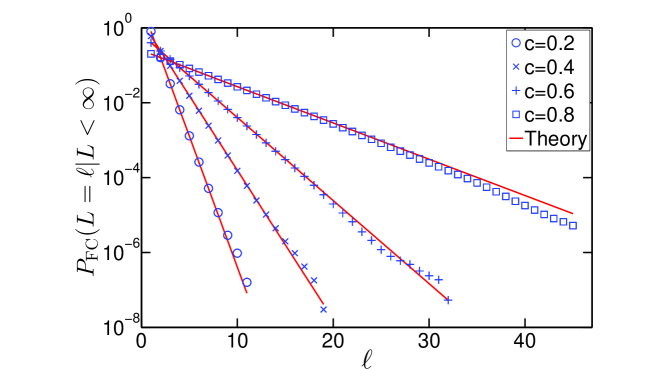
In Fig. 7 we present theoretical results for the DSPL of asymptotic ER networks with $c=0.2,0.4,0.6$ and $0.8$ (solid lines), obtained from Eq. (95). These results are compared to numerical results for the DSPL (symbols), obtained for networks of size $N=10^{4}$ and the same four values of $c$. We find that the theoretical results are in very good agreement with the numerical results except for small deviations in the large distance tails. These deviations are due to finite size of the simulated networks. The numerical simulations were performed via sampling of $10^{4}$ independent realizations of ER networks of size $N=10^{4}$ for each value of $c$ Hartmann2015 . For each realization we applied the all pairs shortest paths algorithm from the LEDA C++ library Leda1999 .

Figure 7: (Color online) The DSPLs of subcritical ER network ensembles with $N=10^{4}$ and $c=0.2,0.4,0.6$ and $0.8$. The theoretical results for the corresponding asymptotic networks (solid lines), obtained from Eq. (95) are in very good agreement with the numerical simulations (symbols). The deviations in the tail are due to the finite size of the sampled networks.

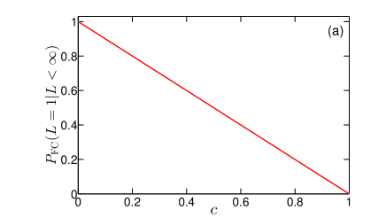
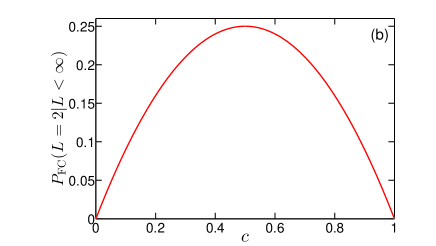
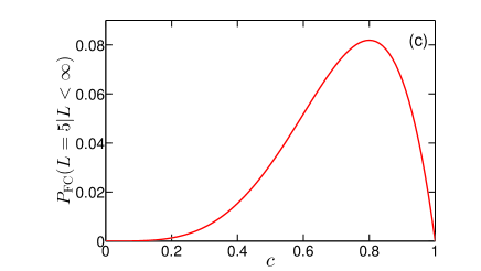
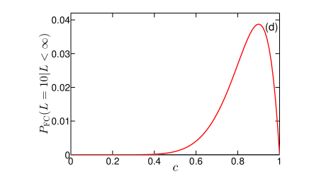
In Fig. 8 we present the probability $P_{\rm FC}(L=\ell|L<\infty)$, given by Eq. (95), as a function of the mean degree, $c$, for $\ell=1,2,5$ and $10$. The probability $P_{\rm FC}(L=1|L<\infty)$ is a monotonically decreasing function of $c$. This is due to the fact that for very low values of $c$ most of the components consisting of two or more nodes are dimers and their fraction decreases as $c$ is increased. For $\ell\geq 2$, the probability $P_{\rm FC}(L=\ell|L<\infty)$ vanishes at $c=0$ and $c=1$. It increases for low values of $c$, reaches a peak and then starts to decrease. For each value of $\ell\geq 2$, the peak of $P_{\rm FC}(L=\ell|L<\infty)$ is located at $c=1-1/\ell$, reflecting the appearance of longer paths as $c$ is increased.

Figure 8: (Color online) The probability $P_{\rm FC}(L=\ell|L<\infty)$ given by Eq. (95), is shown as a function of the mean degree, $c$, for $\ell=1,2,5$ and $10$. The probability $P_{\rm FC}(L=1|L<\infty)$ is a monotonically decreasing function of $c$. For $\ell\geq 2$, the probability $P_{\rm FC}(L=\ell|L<\infty)$ exhibits a peak at $c=1-1/\ell$, which is the value of $c$ at which the probability of two random nodes to be at a distance $\ell$ from each other is maximal.

It is also interesting to consider the conditional probabilities $P_{\rm FC}(L=\ell|L<\infty,K=k)$ and $P_{\rm FC}(L=\ell|L<\infty,K=k,K^{\prime}=k^{\prime})$, between random pairs of nodes that reside on the same finite component, under the condition that the degrees of one or both nodes are specified, respectively. In supercritical networks, the paths between nodes of high degrees tend to shorter than between nodes of low degrees. This is due to the fact that higher degrees open more paths between the nodes, increasing the probability of short paths to emerge. The situation in subcritical networks is completely different. Any pair of nodes, $i$ and $j$, that reside on the same component are connected by a single path. Such path goes through one neighbor of $i$ and one neighbor of $j$. Therefore, the statistics of the path lengths between pairs of nodes that reside on the same component in subcritical ER networks do not depend on the degrees of these nodes. As a result, the conditional DSPLs satisfy

$$P_{\rm FC}(L=\ell|L<\infty,K=k)=(1-c)c^{\ell-1},$$ (100)

regardless of the value of $k$, and

$$P_{\rm FC}(L=\ell|L<\infty,K=k,K^{\prime}=k^{\prime})=(1-c)c^{\ell-1},$$ (101)

regardless of the values of $k$ and $k^{\prime}$. It is worth pointing out, however, that the probability that a random node of a specified degree, $k$, and another random node of an unspecified degree reside on the same component is dependent on the degree, $k$. Using the results of Appendix B it can be shown that

$$P_{\rm FC}(L<\infty|K=k)=\frac{k}{(1-c)N}.$$ (102)

Similarly, it can be shown that the probability that a random node of degree $k$ and another random node of degree $k^{\prime}$ reside on the same component is given by

$$P_{\rm FC}(L<\infty|K=k,K^{\prime}=k^{\prime})=\frac{kk^{\prime}}{c(1-c)N}.$$ (103)

The DSPL of Eq. (95) applies not only for subcritical ER networks but also for the finite components of supercritical ER networks. According to the duality relations, given a supercritical ER network of $N$ nodes and mean degree $c>1$, the subnetwork that consists of the finite components is a subcritical ER network of size

$$N^{\prime}=Nf(c),$$ (104)

and mean degree

$$c^{\prime}=cf(c),$$ (105)

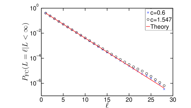
where $f(c)=-{\mathcal{W}(-ce^{-c})}/{c}$ is the fraction of nodes in the supercritical network that reside on the finite components and $c^{\prime}<1$. In Fig. 9 we present numerical results for the DSPL of the finite components of a supercritical ER network of $N=10^{4}$ nodes and $c=1.547$ (circles). The results are found to be in very good agreement with numerical results for its dual network, which consists of $N^{\prime}=3882$ nodes and $c^{\prime}=0.6$ ($\times$) and with the analytical results for an asymptotic subcritical ER network with $c=0.6$ (solid line), obtained from Eq. (95).

Figure 9: (Color online) Numerical results for the DSPL on the finite components of an ${\rm ER}[N,c/(N-1)]$ network with $N=10^{4}$ and $c=1.547$, above percolation (circles) and on its dual network, ${\rm ER}[N^{\prime},c^{\prime}/(N^{\prime}-1)]$ where $N^{\prime}=3882$ [obtained from Eq. (104)] and $c^{\prime}=0.6$ [obtained from Eq. (105)], below percolation ($\times$), which are essentially identical and in excellent agreement with the theoretical results (solid line), obtained from Eq. (95).

VIII The mean and variance of the DSPL

The moments of the DSPL provide useful information about the large scale structure of the network. The first and second moments are of particular importance. The first moment, $\langle L\rangle_{\rm FC}$ provides the mean distance. The width of the DSPL is characterized by the variance, ${\rm Var}(L)=\langle L^{2}\rangle-\langle L\rangle^{2}$, where $\langle L^{2}\rangle$ is the second moment.

The $n^{\rm th}$ moment of the DSPL over all trees of size $s$ and topology $\tau$ is given by

$${\mathbb{E}}[L^{n}|\tau;L<\infty,S=s]=\sum_{\ell=1}^{s-1}\ell^{n}P_{\rm FC}(L=\ell|\tau;L<\infty,S=s),$$ (106)

where $P_{\rm FC}(L=\ell|\tau;L<\infty,S=s)$ is given by Eq. (91). The $n^{\rm th}$ moment of the DSPL over trees of all topologies, which consist of $s$ nodes is given by

$${\mathbb{E}}[L^{n}|S=s]=\frac{\sum\limits_{\{\tau|s\}}X(\tau)W(\tau;s){\mathbb{E}}[L^{n}|\tau;L<\infty,S=s]}{\sum\limits_{\{\tau|s\}}X(\tau)W(\tau;s)},$$ (107)

where ${\mathbb{E}}[L|\tau;L<\infty,S=s]$ is given by Eq. (106).

The results for the first two moments, ${\mathbb{E}}[L|S=s]$ and ${\mathbb{E}}[L^{2}|S=s]$, and for the variance ${\rm Var}[L|S=s]={\mathbb{E}}[L^{2}|S=s]-({\mathbb{E}}[L|S=s])^{2}$, for $s=2,3,\dots,10$ are shown in Table 5.

The $n^{\rm th}$ moment of the DSPL over all trees that consist of up to $s$ nodes is given by

$${\mathbb{E}}[L^{n}|S\leq s]=\frac{\sum\limits_{s^{\prime}=2}^{s}\binom{s^{\prime}}{2}P_{\rm FC}(S=s^{\prime}){\mathbb{E}}[L^{n}|S=s^{\prime}]}{\sum\limits_{s^{\prime}=2}^{s}\binom{s^{\prime}}{2}P_{\rm FC}(S=s^{\prime})},$$ (108)

where $P_{\rm FC}(S=s^{\prime})$ is given by Eq. (127) and ${\mathbb{E}}[L^{n}|S=s^{\prime}]$ is given by Eq. (107). Performing the summation over all tree topologies up to size $s$ provides exact analytical expressions for the moments of the DSPL over these trees. The results for ${\mathbb{E}}[L|S\leq s^{\prime}]$ and ${\mathbb{E}}[L^{2}|S\leq s^{\prime}]$ For small trees of sizes $s=2,3,\dots,6$ are shown in Table 6. In the limit of large $s$, the mean distance ${\mathbb{E}}[L|S\leq s]$ converges towards the asymptotic result, which is given by

$$\langle L\rangle_{\rm FC}=\frac{1}{1-c}.$$ (109)

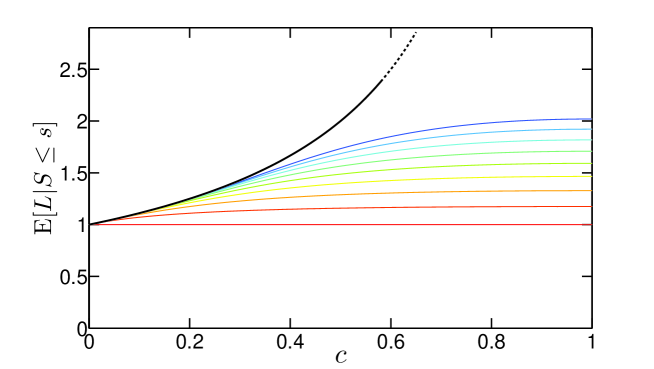
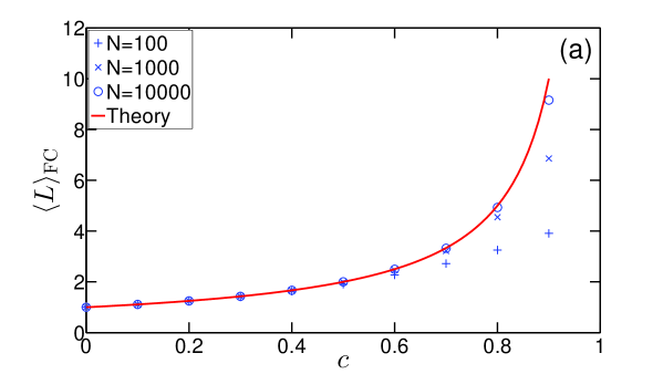
In Fig. 10 we present the mean distances ${\mathbb{E}}[L|S\leq s]$ (solid lines) over all tree topologies of sizes smaller or equal to $s$, as a function of $c$, for $s=2,3,\dots,10$ (from bottom to top, respectively). The thick solid line shows the asymptotic result, $\langle L\rangle_{\rm FC}$, given by Eq. (109). Clearly, as the tree size, $s$, is increased, ${\mathbb{E}}[L|S\leq s]$ approaches the asymptotic result. As expected, for $c\ll 1$ the convergence is fast, but as $c$ approaches the percolation threshold, the asymptotic result diverges and the convergence slows down.

Figure 10: (Color online) The mean distance ${\mathbb{E}}[L|S\leq s]$, over all tree topologies of sizes smaller or equal to $s$, as a function of $c$, for $s=2,3,\dots,10$ (solid lines), from bottom to top, respectively. The thick solid line shows the asymptotic result, $\langle L\rangle_{\rm FC}$.

Using Eq. (108) one can obtain exact analytical expressions for the second moment of the DSPL over all trees of size $S\leq s$. The results for small trees that consist of up to $s=2,3,\dots,6$ nodes are shown in Table 6. In the limit of large $s$, the second moment ${\mathbb{E}}[L^{2}|S\leq s]$ converges towards the asymptotic result, which is given by

$$\langle L^{2}\rangle_{\rm FC}=\frac{1+c}{(1-c)^{2}}.$$ (110)

The variance of the DSPL over all trees that consist of up to $s$ nodes is given by

$${\rm Var}[L|S\leq s]={\mathbb{E}}[L^{2}|S\leq s]-({\mathbb{E}}[L|S\leq s])^{2}.$$ (111)

Using the results presented in Table 6 for the first and second moments of the degree distributions over small trees of sizes $s=2,3,\dots,5$, we obtain

$${\rm Var}[L|S\leq 2] = 0$$

$${\rm Var}[L|S\leq 3] = \frac{\eta+2\eta^{2}}{(1+3\eta)^{2}}$$

$${\rm Var}[L|S\leq 4] = \frac{\eta+9\eta^{2}+19\eta^{3}+31\eta^{4}}{\left(1+3\eta+8\eta^{2}\right)^{2}}$$

$${\rm Var}[L|S\leq 5] = \frac{36\eta+324\eta^{2}+1854\eta^{3}+4044\eta^{4}+7950\eta^{5}+12054\eta^{6}}{\left(6+18\eta+48\eta^{2}+125\eta^{3}\right)^{2}}.$$ (112)

In the limit of large $s$, the variance ${\rm Var}[L|S\leq s]$ converges towards the asymptotic result, $\sigma^{2}_{L,{\rm FC}}={\rm Var}(L)$, where $\sigma_{L,{\rm FC}}$ is the standard deviation of the DSPL over all the finite components. The asymptotic variance is given by

$${\rm Var}(L)=\langle L^{2}\rangle_{\rm FC}-\langle L\rangle_{\rm FC}^{2}.$$ (113)

Using Eqs. (109) and (110) we find that

$$\sigma^{2}_{L,{\rm FC}}={\rm Var}(L)=\frac{c}{(1-c)^{2}}.$$ (114)

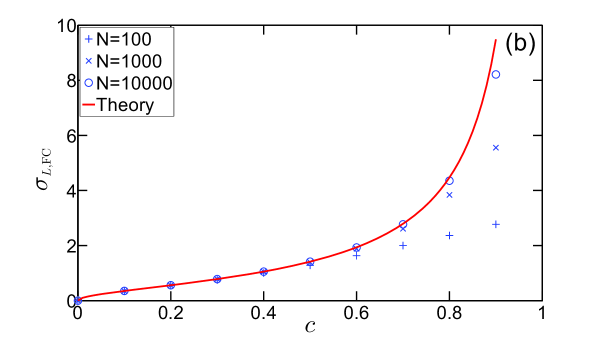
In Fig. 11 we present the mean distance, $\langle L\rangle_{\rm FC}$ (a), and the standard deviation $\sigma_{L,{\rm FC}}$ (b), vs. the mean degree, $c$. The theoretical results (solid lines) correspond to the asymptotic limit. The numerical results, obtained for $N=10^{2}$ ($+$), $10^{3}$ ($\times$) and $10^{4}$ ($\circ$) are found to converge towards the theoretical results as the network size is increased.

Figure 11: (Color online) The mean, $\langle L\rangle_{\rm FC}$ (a), and the standard deviation, $\sigma_{L,{\rm FC}}$ (b), of the DSPL of a subcritical ER network vs. the mean degree, $c$. The numerical results (symbols) for $N=10^{2}$, $10^{3}$ and $10^{4}$ clearly converge towards the analytical results (solid lines).

IX Discussion

Apart from the shortest path length, random networks exhibit other distance measures such as the resistance distance Deza2009 ; Derrida1982 ; Bapat2014 . The resistance distance, $r_{ij}$, between a pair of nodes, $i$ and $j$ is the electrical resistance between them under conditions in which each edge in the network represents a resistor of $1$ Ohm. Unlike the shortest path length, the resistance distance depends on all the paths between $i$ and $j$, which often merge and split along the way. It can be evaluated using the standard rules under which the total resistance of resistors connected in series is the sum of their individual resistance values, while the total resistance of resistors connected in parallel is the reciprocal of the sum of the reciprocals of the individual resistance values. It was shown that the resistance distance between nodes $i$ and $j$ in a network can be decomposed in terms of the eigenvalues and eigenvectors of the normalized Laplacian matrix of the network Chen2007 ; Yang2013 . In order to utilize this result for the calculation of the full distribution of resistance distances, $P(R=r)$, in an ensemble of supercritical ER networks, one will need to obtain the full statistics of the spectral properties of the Laplacian matrix over the ensemble, which is expected to be a difficult task. For subcritical ER networks the situation is simpler. Since the finite components in subcritical networks are trees, the shortest path between a pair of nodes, $i$ and $j$, is in fact the only path between them. As a result, the resistance distance between $i$ and $j$ is equal to the shortest path length between them. This means that the results presented in this paper provide not only the distribution of shortest path lengths in subcritical ER networks but also the distribution of resistance distances in these networks, which is given by

$$P_{\rm FC}(R=r|R<\infty)=(1-c)c^{r-1},$$ (115)

where $r$ takes integer values.

Another distance measure between nodes in random networks is the mean first passage time, $t_{ij}$, of a random walk (RW) starting from node $i$ and reaching node $j$ Sood2005 ; Debacco2015 . Unlike the shortest path length, the mean first passage time is not symmetric, namely $t_{ij}\neq t_{ji}$. Since a RW may wander through side branches, the mean first passage time cannot be shorter than the shortest path, namely $t_{ij}\geq\ell_{ij}$. However, apart from this inequality, there is no simple way to connect between these two quantities. Therefore, numerical simulations will be suitable here. Using specific large-deviation algorithms Hartmann2002 ; Hartmann2014 , it is possible, in principle, to sample the distributions over its full support, i.e. down to very small probabilities like $10^{-100}$. Such approaches have been already applied to obtain distributions of several properties of random graphs, e.g., the distribution of the number of components Engel2004 , the distribution of the size of the largest component Hartmann2011 , the distribution of the 2-core size Hartmann2017b or the distribution of the diameters Hartmann2017 .

Unlike RWs, which would eventually visit all the nodes in the component on which they reside, the paths of self avoiding walks (SAWs) terminate once they enter a leaf node Tishby2016 . Therefore, an SAW starting from node $i$ does not necessarily reach node $j$ even if they reside on the same component. However, in case it reaches node $j$ its first passage time is equal to the shortest path length between $i$ and $j$. Therefore, the distribution of first passage times, $P_{\rm SAW}(T=t|T<\infty)$, of SAWs between pairs of nodes that reside on the same component satisfies $P_{\rm SAW}(T=t|T<\infty)=P_{\rm FC}(L=\ell|L<\infty)$.

The DSPL of subcritical ER networks is also relevant to the study of epidemic spreading on supercritical ER networks. Consider a supercritical ER network with mean degree $c>1$. An epidemic starts from a random node, $i$, and propagates through the shell structure around this node. The time is discrete, so each node that is infected at time $t$ may infect each one of its neighbors at time $t+1$, with probability $p^{\prime}$. The node that was infected at time $t$ recovers at time $t+1$ and becomes immune.

The expectation value of the number of nodes infected by node $i$ in the first time step is given by $c^{\prime}=cp^{\prime}$. In case that $c^{\prime}<1$, the statistical properties of the components formed by such epidemic are similar to the statistical properties of the tree components in a subcritical network with mean degree $c^{\prime}$. More precisely, the size distribution of components formed by the epidemic follows the distribution $P_{\rm FC}(S=s)$ of component sizes on which a random node resides, given by Eq. (128). This property represents some kind of invariance, the distribution of epidemic sizes depends only on the value of the product $c^{\prime}=cp^{\prime}$ rather than the values of $c$ and $p^{\prime}$ alone. The DSPL, $P_{\rm FC}(L=\ell|L<\infty)$ represents the temporal propagation of a typical epidemic, namely the probability that a node that was infected by an epidemic got infected $ell$ time steps after the epidemic started.

Using extreme value statistics it may be possible to obtain analytical results for the distributions of radii and diameters over all the tree topologies. For networks that satisfy duality relations, it will be possible to obtain the DSPL on the finite components in the supercritical regime. Combining the results with the DSPL on the giant component will yield the overall DSPL of the supercritical network. The detailed understanding of the DSPL in terms of the topological expansion is expected to be useful in the study of dynamical processes such as epidemic spreading. Since epidemic spreading and many other real-world dynamical processes take place on networks that are different from ER networks, it will be interesting to apply the topological expansion presented here to the analysis of the DSPL in a broader class of subcritical random networks. In particular, extending this approach to configuration model networks will provide the DSPL of subcritical random networks with any desired degree distribution. To this end, one will need to derive an equation for the size distribution of the finite tree components, $P_{\rm FC}(S=s)$ in a configuration model network with a given degree distribution, $P(K=k)$. The weights, $W(\tau;s)$, of the different tree topologies, $\tau$, which consist of $s$ nodes, in a configuration model network are expected to depend on the degree distribution. Therefore, one will need to derive an equation for $W(\tau,s)$ in terms of $P(K=k)$. Once the weights become available, the counting of the shortest paths follows the same procedure used in the ER case. It will also be interesting to apply the topological expansion to edge-independent, inhomogeneous random graphs Chung2003 ; Bollobas2007 ; Lu2013 . This family of network models provides a generalization of the ER network, in which the probability $p$ is replaced by a random $N\times N$ matrix, ${\mathcal{P}}$, in which the matrix element ${\mathcal{P}}_{ij}$ is the probability that nodes $i$ and $j$ are connected by an edge. As a result, each node, $i$, exhibits unique statistical properties that depend on ${\mathcal{P}}_{ij}$, $j=1,2,\dots,N$, leading to non-Poissonian degree distributions, as in the case of configuration model networks. To apply the topological expansion to inhomogeneous random graphs one will need to perform an additional summation over the distribution of the matrix elements of ${\mathcal{P}}$.

X Summary

We have developed a topological expansion methodology for the analysis of subcritical random networks. The expansion is based on the fact that such networks are fragmented into finite tree components, which can be classified systematically by their sizes and topologies. Using this approach we performed a systematic calculation of the degree distribution, $P_{\rm FC}(K=k|S\leq s)$, and the DSPL $P_{\rm FC}(L=\ell|L<\infty,S\leq s)$, over all components whose size is smaller or equal to $s$, in subcritical ER networks. Taking the large $s$ limit, we obtained an exact asymptotic formula for the DSPL over all pairs of nodes that reside on the same component, which takes the form

$$P_{\rm FC}(L=\ell|L<\infty)=(1-c)c^{\ell-1}.$$ (116)

This remarkably simple asymptotic result is obtained only when the contributions of the tree components of all sizes and topologies are taken into account. Such mean-field like results are normally expected to represent the shell structure around a typical node. However, in subcritical networks there is no typical node because the shell structure strongly depends on the size and topology of the tree component in which each node resides as well as on its location in that component.

From the degree distribution and the DSPL, we obtained analytical results for the mean degree, the variance of the degree distribution, the mean distance and the variance of the DSPL over all components whose size is smaller or equal to $s$. Taking the large $s$ limit, we found that the mean path length between all pairs of nodes that reside on the same component is given by

$$\langle L\rangle_{\rm FC}=\frac{1}{1-c}.$$ (117)

As the percolation threshold is approached from below, at $c\rightarrow 1^{-}$, the mean distance diverges as $\langle L\rangle_{\rm FC}\sim(1-c)^{-\alpha}$, where the exponent $\alpha=1$. From the duality relations between a subcritical ER network and the finite components in a corresponding supercritical ER network, it is found that the same exponent, $\alpha=1$, appears also above the transition.

Appendix A The distribution of tree sizes

In this Appendix we review some useful results on the distribution of tree sizes in subcritical ER networks. Consider a subcritical ER network of $N$ nodes with mean degree $c<1$. The expectation value of the number of trees of $s$ nodes in such network is denoted by $T_{s}^{N}$. Using the theory of branching processes, it was shown that $T_{s}^{N}$ is given by Bollobas2001 ; Durrett2007

$$T_{s}^{N}=N{\binom{N}{s}}s^{s-2}\left(\frac{c}{N}\right)^{s-1}\left(1-\frac{c}{N}\right)^{{\binom{s}{2}}-(s-1)}\left(1-\frac{c}{N}\right)^{s(N-s)},$$ (118)

where the binomial coefficient accounts for the number of ways to pick $s$ nodes out of $N$ in order to form a component of size $s$ and the factor of $s^{s-2}$ is the number of distinct tree structures that can be constructed from $s$ distinguishable nodes Cayley1889 . The factor of $(c/N)^{s-1}$ accounts for the probability that the $s$ nodes of the component will be connected by $s-1$ edges. The next term is the probability that there are no other edges connecting pairs of nodes in the component, while the last term is the probability that there are no edges connecting nodes in the components with nodes in the rest of the network. For $s\ll N$ one can approximate the binomial coefficient by $N^{s}/s!$ and obtain

$$T_{s}^{N}=N\frac{s^{s-2}c^{s-1}}{s!}\left(1-\frac{c}{N}\right)^{s(N-s)+{\binom{s}{2}}-(s-1)}.$$ (119)

Since we consider subcritical ER networks, for which $c<1$, unless the network is extremely small the condition $c\ll N$ is satisfied. Therefore, one can approximate the last term in Eq. (119) by an exponential, and obtain

$$T_{s}^{N}=N\frac{s^{s-2}c^{s-1}e^{-cs}}{s!}\exp\left[\frac{c(s^{2}+3s-2)}{2N}\right].$$ (120)

Finally, in the asymptotic limit of $N\rightarrow\infty$, the exponential converges towards $1$ and the expression for the expected number of tree components of $s$ nodes is reduced to Bollobas2001 ; Durrett2007

$$T_{s}^{N}\simeq N\frac{s^{s-2}{c^{s-1}}e^{-cs}}{s!}.$$ (121)

In the limit of large $s$, one can use the Stirling approximation and obtain

$$T_{s}^{N}\simeq\frac{N}{\sqrt{2\pi}c}\frac{e^{-s/s_{\rm max}}}{s^{5/2}},$$ (122)

where the cutoff parameter $s_{\rm max}$ is given by

$$s_{\rm max}=\frac{1}{\ln\left(\frac{1}{ce^{1-c}}\right)}.$$ (123)

As the percolation threshold is approached from below, for $c\rightarrow 1^{-}$, the cutoff parameter diverges, according to $s_{\rm max}\sim 1/(1-c)^{2}$. The expected number of trees of size $s$ per node, obtained from Eq. (122) scales like $T_{s}^{N}/N\propto s^{-\tau}$, where $\tau=5/2$. This is in agreement with the critical component size distribution on regular lattices above the upper critical dimension of $D=6$, where $\tau$ is the Fisher exponent Stauffer2003 , exemplifying the connection between percolation transitions on random networks and regular lattices of high dimensions.

The total number of tree components in a subcritical ER network of $N$ nodes and $c<1$ is denoted by

$$N_{T}(c)=\sum_{s=1}^{N}T_{s}^{N}.$$ (124)

Carrying out the summation, using the expression for $T_{s}^{N}$ from Eq. (121), we obtain that for $0\leq c\leq 1$

$$N_{T}(c)=\left(1-\frac{c}{2}\right)N,$$ (125)

namely $N_{T}(c)$ is a linear, monotonically decreasing function of $c$, where $N_{T}(c=0)=N$ and $N_{T}(c=1)=N/2$. The mean tree size is thus given by

$$\langle S\rangle_{\rm FC}=\frac{2}{2-c},$$ (126)

which does not diverge as $c$ approaches the percolation threshold. Using Eqs. (121) and (125) we can write down the distribution of tree sizes, which takes the form

$$P_{\rm FC}(S=s)=\frac{2s^{s-2}c^{s-1}e^{-cs}}{(2-c)s!}.$$ (127)

In various processes on networks components are selected by by drawing random nodes and choosing the components on which they reside. The probability that a randomly selected node resides on a tree of size $s$ is given by

$$\widetilde{P}_{\rm FC}(S=s)=\frac{s}{\langle S\rangle_{\rm FC}}P_{\rm FC}(S=s).$$ (128)

The mean of this distribution is

$$\langle\widetilde{S}\rangle_{\rm FC}=\frac{\langle S^{2}\rangle_{\rm FC}}{\langle S\rangle_{\rm FC}}=\frac{1}{1-c}.$$ (129)

Thus, as $c\rightarrow 1^{-}$, the mean tree size on which a random node resides diverges.

Consider a random pair of nodes that reside on the same component. The probability that they reside on a component of size $s$ is given by

$$\widehat{P}_{\rm FC}(S=s)=\frac{\binom{s}{2}P_{\rm FC}(S=s)}{\left\langle\binom{S}{2}\right\rangle_{\rm FC}}.$$ (130)

Evaluating the denominator we obtain

$$\left\langle\binom{S}{2}\right\rangle_{\rm FC}=\frac{c}{(1-c)(2-c)}.$$ (131)

The mean of $\widehat{P}_{\rm FC}(S=s)$ is found to be

$$\langle\widehat{S}\rangle_{\rm FC}=\frac{2-c}{(1-c)^{2}},$$ (132)

which diverges quadratically as $c\rightarrow 1^{-}$.

Appendix B The probability that two random nodes reside on the same component

In this Appendix we calculate the probability, $P_{\rm FC}(L<\infty)$, that two random nodes in a subcritical ER network reside on the same component. This probability is given by

$$P_{\rm FC}(L<\infty)=\frac{\mathcal{L}(N,c)}{{\binom{N}{2}}},$$ (133)

where $\mathcal{L}(N,c)$ is the number of pairs of nodes that reside on the same component. It is given by

$$\mathcal{L}(N,c)=\sum_{s\geq 1}{\binom{s}{2}}T_{s}^{N},$$ (134)

where $T_{s}^{N}$ is the number of tree components of size $s$, given by Eq. (121). In order to evaluate this sum we use properties of the Lambert $W$ function, denoted by $\mathcal{W}(x)$ Olver2010 . In particular, we use the implicit definition (Eq. 4.13.1 in Ref. Olver2010 ):

$$\mathcal{W}(x)=xe^{-\mathcal{W}(x)}.$$ (135)

We also use the series expansion (Eq. 4.13.5 in Ref. Olver2010 ):

$$\mathcal{W}(x)=-\sum_{s=1}^{\infty}\frac{s^{s-2}}{s!}s(-x)^{s}.$$ (136)

Using the series expansion of Eq. (136) it can be shown that

$$\sum_{s=1}^{\infty}{\binom{s}{2}}\frac{s^{s-2}}{s!}(-x)^{s}=\frac{1}{2}\left[\mathcal{W}(x)-x\frac{d}{dx}\mathcal{W}(x)\right]$$ (137)

Plugging in Eq. 4.13.4 of Ref. Olver2010 , which can be expressed in the form

$$\frac{d}{dx}\mathcal{W}(x)=\frac{\mathcal{W}(x)}{x\left[1+\mathcal{W}(x)\right]},$$ (138)

we obtain

$$\sum_{s=1}^{\infty}{\binom{s}{2}}\frac{s^{s-2}}{s!}(-x)^{s}=\frac{[\mathcal{W}(x)]^{2}}{2\left[1+\mathcal{W}(x)\right]}.$$ (139)

Plugging in $x=-ce^{-c}$, multiplying by $N/c$ and using the representation of $T_{s}^{N}$ in Eq. (121), we obtain for the left-hand side

$$\frac{N}{c}\sum_{s=1}^{\infty}{\binom{s}{2}}\frac{s^{s-2}}{s!}(ce^{-c})^{s}=\sum_{s=1}^{\infty}{\binom{s}{2}}N\frac{s^{s-2}c^{s-1}e^{-cs}}{s!}=\sum_{s=1}^{\infty}{\binom{s}{2}}T_{s}^{N}\,,$$ (140)

which is the quantity we want, for finite values of $N$. Therefore, we obtain

$$\mathcal{L}(N,c)=\left(\frac{N}{2c}\right)\frac{[\mathcal{W}(-ce^{-c})]^{2}}{1+\mathcal{W}(-ce^{-c})}.$$ (141)

For $0<c<1$ it can be shown that $\mathcal{W}(-ce^{-c})=-c$, and thus

$$\mathcal{L}(N,c)=\frac{Nc}{2(1-c)}.$$ (142)

Using Eq. (133) we find that in the asymptotic limit, $N\rightarrow\infty$, the probability that two randomly selected nodes in the network reside on the same component is given by

$$P_{\rm FC}(L<\infty)=\frac{c}{(1-c)(N-1)}\simeq\frac{c}{(1-c)N}.$$ (143)

Table 1: The different degree distributions and DSPLs for the finite components (FC) of subcritical ER networks and the equations which are used to evaluate them.

Distribution	Equation	Description
$P_{\rm FC}(K=k|\tau;S=s)$	Eq. (51)	Degree distribution over all trees of $s$ nodes and topology $\tau$
$P_{\rm FC}(K=k|S=s)$	Eq. (52)	Degree distribution over all trees of $s$ nodes
$P_{\rm FC}(K=k|S\leq s)$	Eq. (53)	Degree distribution over all trees of up to $s$ nodes
$P_{\rm FC}(K=k)$	Eq. (56)	Degree distribution over all trees
${\mathbb{E}}[K|\tau;S=s]$	Eq. (58)	Mean degree over all trees of $s$ nodes and topology $\tau$
${\mathbb{E}}[K|S=s]$	Eq. (59)	Mean degree over all trees of $s$ nodes
${\mathbb{E}}[K|S\leq s]$	Eq. (61)	Mean degree over all trees of up to $s$ nodes
$\langle K\rangle_{\rm FC}$	Eq. (62)	Mean degree over all trees
$P_{\rm FC}(L=\ell|\tau;L<\infty,S=s)$	Eq. (91)	DSPL over all trees of $s$ nodes and topology $\tau$
$P_{\rm FC}(L=\ell|L<\infty,S=s)$	Eq. (92)	DSPL over all trees of $s$ nodes
$P_{\rm FC}(L=\ell|L<\infty,S\leq s)$	Eq. (93)	DSPL over all trees of up to $s$ nodes
$P_{\rm FC}(L=\ell|L<\infty)$	Eq. (95)	DSPL over all trees
${\mathbb{E}}[L|\tau;S=s]$	Eq. (106)	Mean distance over all trees of $s$ nodes and topology $\tau$
${\mathbb{E}}[L|S=s]$	Eq. (107)	Mean distance over all trees of $s$ nodes
${\mathbb{E}}[L|S\leq s]$	Eq. (108)	Mean distance over all trees of up to $s$ nodes
$\langle L\rangle_{\rm FC}$	Eq. (109)	Mean distance over all trees

Table 2: The conditional probabilities $P_{\rm FC}(K=k|S=s)$, that a node selected randomly from all the tree components of size $s$, in a subcritical ER network, will have a degree $k$. Results are shown for $s=2,3,\dots,10$ nodes.

	$s=2$	$s=3$	$s=4$	$s=5$	$s=6$	$s=7$	$s=8$	$s=9$	$s=10$
$P_{\rm FC}(K=1|S=s)$ =	$1$	$\frac{2}{3}$	$\frac{9}{16}$	$\frac{64}{125}$	$\frac{625}{1296}$	$\frac{7776}{16807}$	$\frac{117649}{262144}$	$\frac{2097152}{4782969}$	$\frac{43046721}{100000000}$
$P_{\rm FC}(K=2|S=s)=$		$\frac{1}{3}$	$\frac{3}{8}$	$\frac{48}{125}$	$\frac{125}{324}$	$\frac{6480}{16807}$	$\frac{50421}{131072}$	$\frac{1835008}{4782969}$	$\frac{4782969}{12500000}$
$P_{\rm FC}(K=3|S=s)=$			$\frac{1}{16}$	$\frac{12}{125}$	$\frac{25}{216}$	$\frac{2160}{16807}$	$\frac{36015}{262144}$	$\frac{229376}{1594323}$	$\frac{3720087}{25000000}$
$P_{\rm FC}(K=4|S=s)=$				$\frac{1}{125}$	$\frac{5}{324}$	$\frac{360}{16807}$	$\frac{1715}{65536}$	$\frac{143360}{4782969}$	$\frac{413343}{12500000}$
$P_{\rm FC}(K=5|S=s)=$					$\frac{1}{1296}$	$\frac{30}{16807}$	$\frac{735}{262144}$	$\frac{17920}{4782969}$	$\frac{45927}{10000000}$
$P_{\rm FC}(K=6|S=s)=$						$\frac{1}{16807}$	$\frac{21}{131072}$	$\frac{448}{1594323}$	$\frac{5103}{12500000}$
$P_{\rm FC}(K=7|S=s)=$							$\frac{1}{262144}$	$\frac{56}{4782969}$	$\frac{567}{25000000}$
$P_{\rm FC}(K=8|S=s)=$								$\frac{1}{4782969}$	$\frac{9}{12500000}$
$P_{\rm FC}(K=9|S=s)=$									$\frac{1}{100000000}$
${\mathbb{E}}[K|S=s]=$	1	$\frac{4}{3}$	$\frac{3}{2}$	$\frac{8}{5}$	$\frac{5}{3}$	$\frac{12}{7}$	$\frac{7}{4}$	$\frac{16}{9}$	$\frac{9}{5}$
${\mathbb{E}}[K^{2}|S=s]=$	1	2	$\frac{21}{8}$	$\frac{76}{25}$	$\frac{10}{3}$	$\frac{174}{49}$	$\frac{119}{32}$	$\frac{104}{27}$	$\frac{99}{25}$
${\rm Var}[K|S=s]=$	$0$	$\frac{2}{9}$	$\frac{3}{8}$	$\frac{12}{25}$	$\frac{5}{9}$	$\frac{30}{49}$	$\frac{21}{32}$	$\frac{56}{81}$	$\frac{18}{25}$

Table 3: The probabilities $P_{\rm FC}(K=k|2\leq S\leq s)$, that a node selected randomly from all the tree components of sizes in the range $2\leq S\leq s$, in a subcritical ER network, will have a degree $k$. Results are shown for $s=2,3,\dots,10$ nodes.

	$s=2$	$s=3$	$s=4$	$s=5$	$s=6$
$P_{\rm FC}(K=1|2\leq S\leq s)$ =	$1$	$\frac{2+2\eta}{2+3\eta}$	$\frac{6+6\eta+9\eta^{2}}{6+9\eta+16\eta^{2}}$	$\frac{24+24\eta+36\eta^{2}+64\eta^{3}}{24+36\eta+64\eta^{2}+125\eta^{3}}$	$\frac{120+120\eta+180\eta^{2}+320\eta^{3}+625\eta^{4}}{120+180\eta+320\eta^{2}+625\eta^{3}+1296\eta^{4}}$
$P_{\rm FC}(K=2|2\leq S\leq s)=$		$\frac{\eta}{2+3\eta}$	$\frac{3\eta+6\eta^{2}}{6+9\eta+16\eta^{2}}$	$\frac{12\eta+24\eta^{2}+48\eta^{3}}{24+36\eta+64\eta^{2}+125\eta^{3}}$	$\frac{60\eta+120\eta^{2}+240\eta^{3}+500\eta^{4}}{120+180\eta+320\eta^{2}+625\eta^{3}+1296\eta^{4}}$
$P_{\rm FC}(K=3|2\leq S\leq s)=$			$\frac{\eta^{2}}{6+9\eta+16\eta^{2}}$	$\frac{4\eta^{2}+12\eta^{3}}{24+36\eta+64\eta^{2}+125\eta^{3}}$	$\frac{20\eta^{2}+60\eta^{3}+150\eta^{4}}{120+180\eta+320\eta^{2}+625\eta^{3}+1296\eta^{4}}$
$P_{\rm FC}(K=4|2\leq S\leq s)=$				$\frac{\eta^{3}}{24+36\eta+64\eta^{2}+125\eta^{3}}$	$\frac{5\eta^{3}+20\eta^{4}}{120+180\eta+320\eta^{2}+625\eta^{3}+1296\eta^{4}}$
$P_{\rm FC}(K=5|2\leq S\leq s)=$					$\frac{\eta^{4}}{120+180\eta+320\eta^{2}+625\eta^{3}+1296\eta^{4}}$
${\mathbb{E}}[K|2\leq S\leq 2]=$	$1$	$\frac{2+4\eta}{2+3\eta}$	$\frac{6+12\eta+24\eta^{2}}{6+9\eta+16\eta^{2}}$	$\frac{24+48\eta+96\eta^{2}+200\eta^{3}}{24+36\eta+64\eta^{2}+125\eta^{3}}$	$\frac{120+240\eta+480\eta^{2}+1000\eta^{3}+2160\eta^{4}}{120+180\eta+320\eta^{2}+625\eta^{3}+1296\eta^{4}}$
${\mathbb{E}}[K^{2}|2\leq S\leq s]=$	$1$	$\frac{2+6\eta}{2+3\eta}$	$\frac{6+18\eta+42\eta^{2}}{6+9\eta+16\eta^{2}}$	$\frac{24+72\eta+168\eta^{2}+380\eta^{3}}{24+36\eta+64\eta^{2}+125\eta^{3}}$	$\frac{120+360\eta+840\eta^{2}+1900\eta^{3}+4320\eta^{4}}{120+180\eta+320\eta^{2}+625\eta^{3}+1296\eta^{4}}$

Table 4: The leading finite size correction terms, ${P_{\rm FC}(K=k|2\leq S\leq s)}/{\pi_{\rm FC}(K=1)}-1\simeq q_{s,k}c^{s-k}$ of Eq. (55) for the degree distribution over all the tree topologies with up to $s$ nodes (except for the case of an isolated node). The distribution $\pi_{\rm FC}(K=k)$, given by Eq. (56), is the degree distribution over the entire subcritical network, except for the isolated nodes. As $s$ is increased the correction decreases as $c^{s-1}$ and $P_{\rm FC}(K=k|2\leq S\leq s)$ converges towards $\pi_{\rm FC}(K=k)$.

	$s=2$	$s=3$	$s=4$	$s=5$	$s=6$	$s=7$	$s=8$	$s=9$	$s=10$
$\frac{P_{\rm FC}(K=1|2\leq S\leq s)}{\pi_{\rm FC}(K=1)}-1\simeq$	$\frac{1}{2}c$	$\frac{7}{6}c^{2}$	$\frac{61}{24}c^{3}$	$\frac{671}{120}c^{4}$	$\frac{9031}{720}c^{5}$	$\frac{3211}{112}c^{6}$	$\frac{2685817}{40320}c^{7}$	$\frac{56953279}{362880}c^{8}$	$\frac{1357947691}{3628800}c^{9}$
$\frac{P_{\rm FC}(K=2|2\leq S\leq s)}{\pi_{\rm FC}(K=2)}-1\simeq$		$-2c$	$-4c^{2}$	$-\frac{25}{3}c^{3}$	$-18c^{4}$	$-\frac{2401}{60}c^{5}$	$-\frac{4096}{45}c^{6}$	$-\frac{59049}{280}c^{7}$	$-\frac{31250}{63}c^{8}$
$\frac{P_{\rm FC}(K=3|2\leq S\leq s)}{\pi_{\rm FC}(K=3)}-1\simeq$			$-3c$	$-\frac{15}{2}c^{2}$	$-18c^{3}$	$-\frac{343}{8}c^{4}$	$-\frac{512}{5}c^{5}$	$-\frac{19683}{80}c^{6}$	$-\frac{12500}{21}c^{7}$
$\frac{P_{\rm FC}(K=4|2\leq S\leq s)}{\pi_{\rm FC}(K=4)}-1\simeq$				$-4c$	$-12c^{2}$	$-\frac{98}{3}c^{3}$	$-\frac{256}{3}c^{4}$	$-\frac{2187}{10}c^{5}$	$-\frac{5000}{9}c^{6}$
$\frac{P_{\rm FC}(K=5|2\leq S\leq s)}{\pi_{\rm FC}(K=5)}-1\simeq$					$-5c$	$-\frac{35}{2}c^{2}$	$-\frac{160}{3}c^{3}$	$-\frac{1215}{8}c^{4}$	$-\frac{1250}{3}c^{5}$
$\frac{P_{\rm FC}(K=6|2\leq S\leq s)}{\pi_{\rm FC}(K=6)}-1\simeq$						$-6c$	$-24c^{2}$	$-81c^{3}$	$-250c^{4}$
$\frac{P_{\rm FC}(K=7|2\leq S\leq s)}{\pi_{\rm FC}(K=7)}-1\simeq$							$-7c$	$-\frac{63}{2}c^{2}$	$-\frac{350}{3}c^{3}$
$\frac{P_{\rm FC}(K=8|2\leq S\leq s)}{\pi_{\rm FC}(K=8)}-1\simeq$								$-8c$	$-40c^{2}$
$\frac{P_{\rm FC}(K=9|2\leq S\leq s)}{\pi_{\rm FC}(K=9)}-1\simeq$									$-9c$

Table 5: The probabilities $P_{\rm FC}(L=\ell|L<\infty,S=s)$ that a pair of random nodes on a random component of size $s$ in a subcritical ER network will be at a distance $\ell$ from each other for small tree component of $s=2,3,\dots,10$ nodes.

	$s=2$	$s=3$	$s=4$	$s=5$	$s=6$	$s=7$	$s=8$	$s=9$	$s=10$
$P_{\rm FC}(L=1|S=s)$ =	$1$	$\frac{2}{3}$	$\frac{1}{2}$	$\frac{2}{5}$	$\frac{1}{3}$	$\frac{2}{7}$	$\frac{1}{4}$	$\frac{2}{9}$	$\frac{1}{5}$
$P_{\rm FC}(L=2|S=s)=$		$\frac{1}{3}$	$\frac{3}{8}$	$\frac{9}{25}$	$\frac{1}{3}$	$\frac{15}{49}$	$\frac{9}{32}$	$\frac{7}{27}$	$\frac{6}{25}$
$P_{\rm FC}(L=3|S=s)=$			$\frac{1}{8}$	$\frac{24}{125}$	$\frac{2}{9}$	$\frac{80}{343}$	$\frac{15}{64}$	$\frac{56}{243}$	$\frac{28}{125}$
$P_{\rm FC}(L=4|S=s)=$				$\frac{6}{125}$	$\frac{5}{54}$	$\frac{300}{2401}$	$\frac{75}{512}$	$\frac{350}{2187}$	$\frac{21}{125}$
$P_{\rm FC}(L=5|S=s)=$					$\frac{1}{54}$	$\frac{720}{16807}$	$\frac{135}{2048}$	$\frac{560}{6561}$	$\frac{63}{625}$
$P_{\rm FC}(L=6|S=s)=$						$\frac{120}{16807}$	$\frac{315}{16384}$	$\frac{1960}{59049}$	$\frac{147}{3125}$
$P_{\rm FC}(L=7|S=s)=$							$\frac{45}{16384}$	$\frac{4480}{531441}$	$\frac{252}{15625}$
$P_{\rm FC}(L=8|S=s)=$								$\frac{560}{531441}$	$\frac{567}{156250}$
$P_{\rm FC}(L=9|S=s)=$									$\frac{63}{156250}$
${\mathbb{E}}[L|S=s]=$	$1$	$\frac{4}{3}$	$\frac{13}{8}$	$\frac{236}{125}$	$\frac{115}{54}$	$\frac{39572}{16807}$	$\frac{42037}{16384}$	$\frac{1469756}{531441}$	$\frac{461843}{156250}$
${\mathbb{E}}[L^{2}|S=s]=$	1	2	$\frac{25}{8}$	$\frac{542}{125}$	$\frac{101}{18}$	$\frac{116582}{16807}$	$\frac{136033}{16384}$	$\frac{1718890}{177147}$	$\frac{1739471}{156250}$
${\rm Var}[L|S=s]=$	$0$	$\frac{2}{9}$	$\frac{31}{64}$	$\frac{12054}{15625}$	$\frac{3137}{2916}$	$\frac{393450490}{282475249}$	$\frac{461655303}{268435456}$	$\frac{580283161934}{282429536481}$	$\frac{58493387101}{24414062500}$

Table 6: The probabilities $P_{\rm FC}(L=\ell|L<\infty,S\leq s)$ that a pair of random nodes on a random component of size $S\leq s$ in a subcritical ER network will be at a distance $\ell$ from each other for small tree components of $s=2,3,\dots,10$ nodes.

	$s=2$	$s=3$	$s=4$	$s=5$	$s=6$
$P_{\rm FC}(L=1|S\leq s)=$	$1$	$\frac{1+2\eta}{1+3\eta}$	$\frac{1+2\eta+4\eta^{2}}{1+3\eta+8\eta^{2}}$	$\frac{6+12\eta+24\eta^{2}+50\eta^{3}}{6+18\eta+48\eta^{2}+125\eta^{3}}$	$\frac{6+12\eta+24\eta^{2}+50\eta^{3}+108\eta^{4}}{6+18\eta+48\eta^{2}+125\eta^{3}+324\eta^{4}}$
$P_{\rm FC}(L=2|S\leq s)=$		$\frac{\eta}{1+3\eta}$	$\frac{\eta+3\eta^{2}}{1+3\eta+8\eta^{2}}$	$\frac{6\eta+18\eta^{2}+45\eta^{3}}{6+18\eta+48\eta^{2}+125\eta^{3}}$	$\frac{6\eta+18\eta^{2}+45\eta^{3}+108\eta^{4}}{6+18\eta+48\eta^{2}+125\eta^{3}+324\eta^{4}}$
$P_{\rm FC}(L=3|S\leq s)=$			$\frac{\eta^{2}}{1+3\eta+8\eta^{2}}$	$\frac{6\eta^{2}+24\eta^{3}}{6+18\eta+48\eta^{2}+125\eta^{3}}$	$\frac{6\eta^{2}+24\eta^{3}+72\eta^{4}}{6+18\eta+48\eta^{2}+125\eta^{3}+324\eta^{4}}$
$P_{\rm FC}(L=4|S\leq s)=$				$\frac{6\eta^{3}}{6+18\eta+48\eta^{2}+125\eta^{3}}$	$\frac{6\eta^{3}+30\eta^{4}}{6+18\eta+48\eta^{2}+125\eta^{3}+324\eta^{4}}$
$P_{\rm FC}(L=5|S\leq s)=$					$\frac{6\eta^{4}}{6+18\eta+48\eta^{2}+125\eta^{3}+324\eta^{4}}$
${\mathbb{E}}[L|S\leq s]=$	$1$	$\frac{1+4\eta}{1+3\eta}$	$\frac{1+4\eta+13\eta^{2}}{1+3\eta+8\eta^{2}}$	$\frac{6+24\eta+78\eta^{2}+236\eta^{3}}{6+18\eta+48\eta^{2}+125\eta^{3}}$	$\frac{6+24\eta+78\eta^{2}+236\eta^{3}+690\eta^{4}}{6+18\eta+48\eta^{2}+125\eta^{3}+324\eta^{4}}$
${\mathbb{E}}[L^{2}|S\leq s]=$	$1$	$\frac{1+6\eta}{1+3\eta}$	$\frac{1+6\eta+25\eta^{2}}{1+3\eta+8\eta^{2}}$	$\frac{6+36\eta+150\eta^{2}+542\eta^{3}}{6+18\eta+48\eta^{2}+125\eta^{3}}$	$\frac{6+36\eta+150\eta^{2}+542\eta^{3}+1818\eta^{4}}{6+18\eta+48\eta^{2}+125\eta^{3}+324\eta^{4}}$

Table 7: The leading finite size correction terms $r_{s,\ell}c^{s-\ell}$ of Eq. (94) for the DSPL over all the tree topologies with up to $s$ nodes. The distribution $P_{\rm FC}(L=\ell|L<\infty)=(1-c)c^{\ell-1}$, given by Eq. (95), is the DSPL over all pairs of nodes that reside on the same component in the entire subcritical network. As $s$ is increased, the correction term decreases as $c^{s-2}$ and $P_{\rm FC}(L=\ell|L<\infty,S\leq s)$ converges towards $P_{\rm FC}(L=\ell|L<\infty)$.

	$s=2$	$s=3$	$s=4$	$s=5$	$s=6$	$s=7$	$s=8$	$s=9$	$s=10$
$\frac{P_{\rm FC}(L=1|L<\infty,S\leq s)}{P_{\rm FC}(L=1|L<\infty)}-1=$	$1$	$4c^{2}$	$\frac{25}{2}c^{3}$	$36c^{4}$	$\frac{2401}{24}c^{5}$	$\frac{4096}{15}c^{6}$	$\frac{59049}{80}c^{7}$	$\frac{125000}{63}c^{8}$	$\frac{214358881}{40320}c^{9}$
$\frac{P_{\rm FC}(L=2|L<\infty,S\leq s)}{P_{\rm FC}(L=2|L<\infty)}-1=$		$-3c$	$-\frac{15}{2}c^{2}$	$-18c^{3}$	$-\frac{343}{8}c^{4}$	$-\frac{512}{5}c^{5}$	$-\frac{19683}{80}c^{6}$	$-\frac{12500}{21}c^{7}$	$-\frac{19487171}{13440}c^{8}$
$\frac{P_{\rm FC}(L=3|L<\infty,S\leq s)}{P_{\rm FC}(L=3|L<\infty)}-1=$			$-4c$	$-12c^{2}$	$-\frac{98}{3}c^{3}$	$-\frac{256}{3}c^{4}$	$-\frac{2187}{10}c^{5}$	$-\frac{5000}{9}c^{6}$	$-\frac{1771561}{1260}c^{7}$
$\frac{P_{\rm FC}(L=4|L<\infty,S\leq s)}{P_{\rm FC}(L=4|L<\infty)}-1=$				$-5c$	$-\frac{35}{2}c^{2}$	$-\frac{160}{3}c^{3}$	$-\frac{1215}{8}c^{4}$	$-\frac{1250}{3}c^{5}$	$-\frac{161051}{144}c^{6}$
$\frac{P_{\rm FC}(L=5|L<\infty,S\leq s)}{P_{\rm FC}(L=5|L<\infty)}-1=$					$-6c$	$-24c^{2}$	$-81c^{3}$	$-250c^{4}$	$-\frac{14641}{20}c^{5}$
$\frac{P_{\rm FC}(L=6|L<\infty,S\leq s)}{P_{\rm FC}(L=6|L<\infty)}-1=$						$-7c$	$-\frac{63}{2}c^{2}$	$-\frac{350}{3}c^{3}$	$-\frac{9317}{24}c^{4}$
$\frac{P_{\rm FC}(L=7|L<\infty,S\leq s)}{P_{\rm FC}(L=7|L<\infty)}-1=$							$-8c$	$-40c^{2}$	$-\frac{484}{3}c^{3}$
$\frac{P_{\rm FC}(L=8|L<\infty,S\leq s)}{P_{\rm FC}(L=8|L<\infty)}-1=$								$-9c$	$-\frac{99}{2}c^{2}$
$\frac{P_{\rm FC}(L=9|L<\infty,S\leq s)}{P_{\rm FC}(L=9|L<\infty)}-1=$									$-10c$

References

- (1) S. Havlin and R. Cohen, Complex networks: structure, robustness and function (Cambridge University Press, New York, 2010).
- (2) M.E.J. Newman, Networks: an introduction (Oxford University Press, Oxford, 2010).
- (3) E. Estrada, The structure of complex networks: theory and applications (Oxford University Press, Oxford, 2011).
- (4) P.A.C. Duijn, V. Kashirin and P.M.A and Sloot, The relative ineffectiveness of criminal network disruption, Sci. Rep. 4, 4238 (2014).
- (5) J. Shao, S.V. Buldyrev, R. Cohen, M. Kitsak, S. Havlin and H.E. Stanley, Fractal boundaries of complex networks, Europhys. Lett. 84, 48004 (2008).
- (6) J. Shao, S.V. Buldyrev, L.A. Braunstein, S. Havlin and H.E. Stanley, Structure of shells in complex networks, Phys. Rev. E 80, 036105 (2009).
- (7) P. Erdős and A. Rényi, On random graphs I, Publicationes Mathematicae (Debrecen) 6, 290 (1959).
- (8) P. Erdős and A. Rényi, On the evolution of random graphs, Publ. Math. Inst. Hung. Acad. Sci. 5, 17 (1960).
- (9) P. Erdős and A. Rényi, On the evolution of random graphs II, Bull. Inst. Int. Stat. 38, 343 (1961).
- (10) B. Bollobás, Random Graphs, Second Edition (Academic Press, London, 2001).
- (11) M.E.J. Newman, S.H. Strogatz and D.J. Watts, Random graphs with arbitrary degree distributions and their applications, Phys. Rev. E 64, 026118 (2001).
- (12) H. Klein-Hennig and A.K. Hartmann, Bias in generation of random graphs, Phys. Rev. E 85, 026101 (2012)
- (13) R. Durrett, Random Graph Dynamics (Cambridge University Press, Cambridge, 2007).
- (14) F.W. Olver, D.W. Lozier, R.F. Boisvert and C.W. Clark, NIST Handbook of Mathematical Functions (Cambridge University Press, Cambridge, 2010).
- (15) F. Chung and L. Lu, The average distances in random graphs with given expected degrees, Proc. Natl. Acad. Sci. USA 99, 15879 (2002).
- (16) R. van der Hofstad, G. Hooghiemstra and P. van Mieghem, Distances in random graphs with finite variance degrees, Rand. Struct. Algo. 27, 76 (2005).
- (17) B. Bollobás, S. Janson and O. Riordan, The phase transition in inhomogeneous random graphs, Rand. Struct. Algo. 31, 3 (2007).
- (18) A. Fronczak, P. Fronczak and J.A. Holyst, Average path length in random networks, Phys. Rev. E 70, 056110 (2004).
- (19) A.K. Hartmann and M. Mézard, Distribution of diameters for Erdős-Rényi random graphs, Phys. Rev. E 97, 032128 (2017).
- (20) S.N. Dorogovtsev, J.F.F. Mendes and A.N. Samukhin, Metric structure of random networks, Nuclear Physics B 653, 307 (2003).
- (21) V.D. Blondel, J.-L. Guillaume, J.M. Hendrickx and R.M. Jungers, Distance distribution in random graphs and application to network exploration, Phys. Rev. E 76, 066101 (2007).
- (22) R. van der Hofstad, G. Hooghiemstra and D. Znamenski, Distances in random graphs with finite mean and infinite variance degrees, Elect. J. Prob. 12, 703 (2007).
- (23) H. van der Esker, R. van der Hofstad and G. Hooghiemstra, Universality for the distance in finite variance random graphs, J. Stat. Phys. 133, 169 (2008).
- (24) E. Katzav, M. Nitzan, D. ben-Avraham, P.L. Krapivsky, R. Kühn, N. Ross and O. Biham, Analytical results for the distribution of shortest path lengths in random networks, EPL 111, 26006 (2015).
- (25) M. Nitzan, E. Katzav, R. Kühn and O. Biham, Distance distribution in configuration-model networks, Phys. Rev. E 93, 062309 (2016).
- (26) S. Melnik and J.P. Gleeson, Simple and accurate analytical calculation of shortest path lengths, arXiv:1604.05521.
- (27) R. Pastor-Satorras, C. Castellano, P.V. Mieghem and A. Vespignani, Epidemic processes in complex networks, Rev. Mod. Phys. 87, 925 (2015).
- (28) F. Bouchet, S. Gupta and D. Mukamel, Thermodynamics and dynamics of systems with long-range interactions, Physica A 389, 4389 (2010).
- (29) A. Barrat, M. Barthélemy and A. Vespignani, Dynamical processes on complex networks (Cambridge University Press, New York, 2008).
- (30) S. Shao, X. Huang, H.E. Stanley and S. Havlin, Percolation of localized attack on complex networks, New J. Phys. 17, 023049 (2015).
- (31) T.A. Schieber, L. Carpi, A. Diaz-Guilera, P.M. Pardalos, C. Masoller and M.G. Ravetti, Quantification of networks structural dissimilarities, Nat. Commun. 8, 13928 (2017).
- (32) L. Giot et al., A protein interaction map of Drosophila melanogaster, Science 302, 1727 (2003).
- (33) H. Bonneau, A. Hassid, O. Biham, R. Kühn and E. Katzav, Distribution of shortest cycle lengths in random networks, Phys. Rev. E 96, 062307 (2017).
- (34) A. Goldental, R. Vardi, S. Sardi, P. Sabo and I. Kanter, Broadband macroscopic cortical oscillations emerge from intrinsic neuronal response failures, Front. Neural Circ. 9, 65 (2015).
- (35) A. Goldental, H. Uzan, S. Sardi and I. Kanter, Oscillations in networks of networks stem from adaptive nodes with memory, Sci. Rep. 7, 2700 (2017).
- (36) R. Cohen and S. Havlin, Scale-free networks are ultrasmall, Phys. Rev. Lett. 90, 058701 (2003).
- (37) M. Molloy and A. Reed, A critical point for random graphs with a given degree sequence, Rand. Struct. Algo. 6, 161 (1995).
- (38) M. Molloy and A. Reed, The size of the giant component of a random graph with a given degree sequence, Combin. Probab. Comput. 7, 295 (1998).
- (39) I. Tishby, O. Biham, E. Katzav and R. Kühn, Revealing the micro-structure of the giant component in random graph ensembles, Phys. Rev. E 97, 042318 (2018).
- (40) B. Gompertz, On the nature of the function expressive of the law of human mortality, and on a new mode of determining the value of life contingencies, Phil. Trans. R. Soc. Lond. A 115, 513 (1825)
- (41) P. Steinbach, Field guide to simple graphs, Volume 3: The book of trees (Design Lab, Albouquerque, 1990).
- (42) R.A. Wright, B. Richmond, A. Odlyzko and B.D. McKay, Constant Time Generation of Free Trees SIAM J. Comput. 15, 540 (1986).
- (43) T. Beyer and S.M. Hedetniemi, Constant Time Generation of Rooted Trees, SIAM J. Comput. 9, 706 (1980).
-
(44)
G. Royle,
Trees On Up to 20 Vertices,
http:school.maths.uwa.edu.augordonremotegraphstrees. - (45) R.P. Stanley, Enumerative combinatorics, Volume I (Cambridge University Press, Cambride, 2011).
- (46) D. Janežič, A. Miličević, S. Nikolić and N. Trinajstić, Graph-theoretical matrices in chemistry (CRC Press, Boca Raton, 2015).
- (47) A.K. Hartmann, Big Practical Guide to Computer Simulations (World scientific, Singapore, 2015).
- (48) K. Mehlhorn and S. Näher, The LEDA Platform of Combinatorial and Geometric Computing (Cambridge University Press, Cambridge, 1999).
- (49) M.M. Deza and E. Deza, Encyclopedia of distances, (Springer, Berlin, 2009).
- (50) B. Derrida and J. Vannimenus, A transfer-matrix approach to random resistor networks, J. Phys. A 15, L557 (1982).
- (51) R.B. Bapat, Graphs and matrices (Springer, London, 2014).
- (52) H. Chen and F. Zhang, Resistance distance and the normalized Laplacian spectrum, Disc. Appl. Math. 155, 654 (2007).
- (53) Y. Yang and D.J. Klein, A recursion formula for resistance distances and its applications, Disc. Appl. Math. 161, 2702 (2013).
- (54) V. Sood, S. Redner and D. ben-Avraham, First-passage properties of the Erdős-Rényi random graph, J. Phys. A 38, 109 (2005).
- (55) C. De Bacco, S.N. Majumdar and P. Sollich, The average number of distinct sites visited by a random walker on random graphs, J. Phys. A 48, 205004 (2015).
- (56) A.K. Hartmann, Sampling rare events: Statistics of local sequence alignments Phys. Rev. E 65, 056102 (2002).
- (57) A.K. Hartmann, High-precision work distributions for extreme nonequilibrium processes in large systems, Phys. Rev. E 89, 052103 (2014).
- (58) A. Engel, R. Monasson and A.K. Hartmann, On large deviation properties of Erdős-Rényi random graphs, J. Stat. Phys. 117, 387 (2004).
- (59) A.K. Hartmann, Large-deviation properties of largest component for random graphs, Eur. Phys. J. B 84, 627 (2011).
- (60) A.K. Hartmann, Large-deviation properties of the largest 2-core component for random graphs, Eur. Phys. J. Special Topics 226, 567 (2017).
- (61) I. Tishby, O. Biham and E. Katzav, The distribution of path lengths of self avoiding walks on Erdős-Rényi networks, J. Phys. A 50, 115001 (2016).
- (62) F. Chung, L. Lu and V. Vu, Spectra of random graphs with given expected degrees, Proc. Natl. Acad. Sci. USA 100, 6313 (2003).
- (63) L. Lu and X. Peng, Spectra of edge-independent random graphs, The Elect. J. Combin. 20, P27 (2013).
- (64) A. Cayley, A theorem on trees, Quart. J. Pure Appl. Math. 23, 376 (1889).
- (65) D. Stauffer and A. Aharony, Introduction to Percolation Theory (Taylor & Francis, London, 2003).