∎
C. H. Lampert, IST Austria, 11email: chl@ist.ac.at
KS(conf): A Light-Weight Test if a ConvNet Operates Outside of Its Specifications††thanks: This work was in parts funded by the European Research Council under the European Union’s Seventh Framework Programme (FP7/2007-2013)/ERC grant agreement no 308036.
Abstract
Computer vision systems for automatic image categorization have become accurate and reliable enough that they can run continuously for days or even years as components of real-world commercial applications. A major open problem in this context, however, is quality control. Good classification performance can only be expected if systems run under the specific conditions, in particular data distributions, that they were trained for. Surprisingly, none of the currently used deep network architectures has a built-in functionality that could detect if a network operates on data from a distribution that it was not trained for and potentially trigger a warning to the human users.
In this work, we describe KS(conf), a procedure for detecting such outside of the specifications operation. Building on statistical insights, its main step is the applications of a classical Kolmogorov-Smirnov test to the distribution of predicted confidence values. We show by extensive experiments using ImageNet, AwA2 and DAVIS data on a variety of ConvNets architectures that KS(conf) reliably detects out-of-specs situations. It furthermore has a number of properties that make it an excellent candidate for practical deployment: it is easy to implement, adds almost no overhead to the system, works with all networks, including pretrained ones, and requires no a priori knowledge about how the data distribution could change.
 |
 |
 |
 |
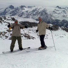
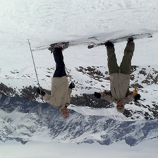
| "ski" | "shovel" | "web site" | "tennis ball" |
1 Introduction
With the emergence of deep convolutional networks (ConvNets), computer vision systems have become accurate and reliable enough to perform tasks of practical relevance autonomously and reliably over long periods of time. This has opened opportunities for the deployment of automated image recognition system in many commercial settings, such as in video surveillance, self-driving vehicles, or social media.
A major concern in our society about automatic decision systems is their reliability: if decisions are made by a trained classifier instead of a person, how can we be sure that the system works reliably now, and that it will continue to do so in the future? Formal verification techniques, as they are common for other safety-critical software components, such as device drivers, are still in their infancy for machine learning. Instead, quality control for trained system typically relies on extensive testing, making use of data that 1) was not used during training, and 2) reflects the expected situation at prediction time. If a system works well on a sufficiently large amount of data fulfilling 1) and 2), practical experience as well as machine learning theory tell us that it will also work well in the future. We call this operating within the specifications (within-specs).
In practice, problems emerge when a chance exists that the data distribution at prediction time differs from our expectations at training time, i.e. when condition 2) is violated. Such operating outside of the specifications (out-of-specs) can happen for a variety of reasons, ranging from user errors, through changing environmental conditions, to problems with the camera setup, and even deliberate sabotage. Standard performance guarantees do not hold anymore in the out-of-specs situations, and the prediction quality often drop substantially.
While this phenomenon is well known in the research community, e.g. under the name of domain shift, and to some extent it is well understood, it remains a major obstacle for the deployment of deep learning system in real-world applications. Surprising as it is, today’s most successful classification architectures, multi-class ConvNets with softmax activation, are not able to tell if they operate inside or outside the specifications. They will, for any input, predict one of the class labels they were trained for, no matter if the external situation matches the training conditions or not. Figure 1 shows an example: a VGG19 ConvNet, trained on ImageNet ILSVRC2012, correctly predicts the label ski for the left-most image. If that image is rotated by 180 degrees, though, e.g. because the camera is mounted upside down, the network classifies it as shovel. As even more extreme examples, a completely black image is classified as web site, and a pattern of random noise as tennis ball.
One can easily imagine many ways for trying to solve this problem, for example, by training the network differently or changing its architecture. However, any method that requires such changes to the training stage strongly reduces its real-world applicability. This is, because training ConvNets requires expert knowledge and large computational resources, so in practice most users rely on pretrained networks, which they use as black boxes, or fine-tune at best. Only the inputs can be influenced and the outputs observed. Sometimes, it might not even be possible to influence the inputs, e.g. in embedded devices, such as smart cameras, or in security related appliances that prevent such manipulations.
It is highly desirable to have a test that can reliably tell when a ConvNet operates out-of-specs, e.g. to send a warning to a human user, but that does not require modifications to any ConvNet internals. Our main contribution in this work is such a test, which is light-weight and theoretically well-founded.
We start in Section 2 by formulating first principles that any test for out-of-specs operation should have. We then describe our proposed method, KS(conf), which has at its core a classical Kolmogorov-Smirnov test that is applied to the confidences of network predictions. KS(conf) fulfills all required criteria and allows for simple and efficient implementation using standard components.
In an extensive experimental evaluation we demonstrate the power of the proposed procedure and show its advantages over alternative approaches. Over the course of these experiments, we obtained a number of insights into the diverse ways by which modern ConvNets reacts to change of their inputs. We find these of independent interest, so we report on a selection of them.
2 Testing for Out-of-Specs Operation
Any test for out-of-specs operation should be able to determine if the conditions under which a classifier currently operates differs from the conditions it was designed for. Assuming a fully automatic system, the only difference that can occur is a change in the input data distribution between training/validation and prediction time. Furthermore, since no ground truth labels are available at prediction time, only changes in the marginal (i.e. input image) distribution will be detectable. These considerations lead to a canonical blueprint for identifying out-of-specs behavior: perform a statistical test if the data observed at prediction time and data from known within-specs operation originate from the same underlying data distribution.
Unfortunately, statistical tests tend to suffer heavily from the curse of dimensionality, so reliable tests between sets of ConvNet inputs (e.g. high-dimensional images) is intractable. Therefore, and because ultimately we are interested in the network predictions anyway, we propose to work with the distribution of network outputs. For a multi-class classifier, the outputs are multi-dimensional, and modeling their distribution might still not be possible. Therefore, we suggest to use only the real-valued confidence value of the predicted label. These values are one-dimensional, available in most practical applications, and as our experiments show, they provide a strong proxy for detecting changes in the distribution of inputs. Because evaluating the network is a deterministic function, the output-based test cannot introduce spurious false positives: if reference and prediction distribution of the inputs are identical, then the distribution of outputs will be identical as well. It would in principle be possible that an output-based test overlooks relevant differences between the input distributions. Our experiments will show, however, that for a well-designed test this does not seem to be the case.
In addition to the probabilistic aspects, a test that aims at practical applications needs to have several additional features. We propose the following necessary conditions that a test must satisfy:
-
•
universal. The same test procedure should be applicable to different network architectures.
-
•
pretrained-ready. The test should be applicable to pretrained and finetuned networks and not require any specific steps during network training.
-
•
black-box ready. The test should not require knowledge of any ConvNet internals, such as the depth, activation functions, or weight matrices.
-
•
nonparametric. The test should not require a priori knowledge how the data distribution could change.
2.1 Notation
We assume an arbitrary fixed ConvNet, , with softmax outputs, i.e. for an input image we obtain an output vector with . Assuming a standard multi-class setting with softmax activation function at the output layer, one has for and . For any output , the predicted class label is , with ties broken arbitrarily. The confidence of this prediction is , i.e. the th entry of the output vector , or equivalently , i.e. the largest entry of .
Treating as a random variable with underlying probability distribution , the other quantities become random variables as well, and we name the induced probability distributions , , and respectively. We are interested in detecting if the distribution at prediction time differs from the distribution when operating within the specifications.
2.2 KS(conf): Kolmogorov-Smirnov Test of Confidences
We suggest a procedure for out-of-specs testing that we call KS(conf), for Kolmogorov-Smirnov test of confidences. Its main component is the application of a Kolmogorov-Smirnov test massey1951kolmogorov to the distribution of confidence values. KS(conf) consists of three main routines: calibration, batch testing and (optionally) filtering.
Calibration.
In this step, we establish a reference distribution for within-specs operation. It is meant to be run when the classifier system is installed at its destination, but a human expert is still available who can ensure that the environment is within-specs for the duration of the calibration phase.
To characterize the within-specs regime, we use a set of validation images, and their corresponding network confidence outputs, . For simplicity we assume all confidence values to be distinct. In practice, this can be enforced by perturbing the values by a small amount of random noise.
The distribution is one-dimensional with known range. Therefore, one can, in principle, estimate its probability density function (pdf) from a reasonably sized set of samples, e.g. by dividing the support into regular bins and counting the fraction of samples falling into each of them. For ConvNet confidence scores this would be wasteful, though, because these scores are typically far from uniformly distributed. To avoid a need for data-dependent binning, KS(conf) starts by a processing step. First, we estimate the inverse cumulative distribution function, , which is possible without binning: we sort the confidence values such that we can assume the values in monotonically increasing order. Then, for any , the estimated inv-cdf value at is obtained by linear interpolation:
| for with , | (1) |
with the convention and .
A particular property of is, that for -distributed , the values are distributed uniformly in . Thus, the quantities we ultimately work with for KS(conf) are the uniformized confidence scores . This transformation will prove useful for two reasons: in the batch testing phase, we will not have to compare two arbitrary distributions to each other, but only the currently observed distribution with the uniform one. In the filtering stage, where we do actually have to perform binning, we can use easier and more efficient uniform bins.
Batch testing.
The main step of KS(conf) is batch testing, which determines at any time of the classifier runtime, if the system operates within-specs or out-of-specs. This step happens at prediction time after the system has been activated to perform its actual task.
Testing is performed on batches of images, , that can but do not have to coincide with the image batches that are often used for efficient ConvNets evaluation on parallel architectures, such as GPUs. To the corresponding network confidences we apply the inverse cdf that was learned during calibration, resulting in values, that, as above, we consider sorted. We then compute the Kolmogorov-Smirnov test statistics
| (2) |
which reflects the biggest absolute difference between the (empirical) cdf of the observed batch, and the linearly increasing reference cdf. For a system that runs within-specs, will be close to uniformly distributed, and can be expected to be small. It will not be exactly , though, because of finite-sample effects and random fluctuations. It is a particularly appealing property of the KS statistics, that its distribution can be derived and used to determine confidence thresholds massey1951kolmogorov : for any there is a threshold , such that if we consider the test outcome positive for , then the expected probability of a false positive test results is . The values can be computed numerically JSSv008i18 or approximated well (in the regime that we are mainly interested in) by .
The Kolmogorov-Smirnov test has several advantages over other tests. In particular, it is distribution-free, i.e. the thresholds are the same regardless of what the distribution was. Also, it is invariant under reparameterization of the sample space, which in particular means that the KS statistics and the test outcome we compute in comparing to the uniform distribution is identical to the one for comparing the original to the within-specs distribution.
Filtering.
A case of particular interest of out-of-specs operation is when the working distribution is almost the reference one, but a certain fraction of unexpected data occurs, e.g. images of object classes that were not present at training time. In such cases, simply send a warning to a human operator might not be sufficient, because the difference in distribution is subtle and might not become clear simply from looking at the input data. We suggest to help the operator by highlighting which of the images in the batch are suspicious and the likely reason to cause the alarm. Unfortunately, on the level of individual samples it is not possible to identify suspicious examples with certainty, except when the support of the reference distribution and the unexpected data are disjoint. Instead, we suggest a filtering approach: if the out-of-specs test is possible, we accompany the warning it with a small number of example images from the batch that triggered the warning. The example images should be chosen in a way to contain as high a fraction of samples from the unexpected component as possible.
In KS(conf), we propose to use a density ratio criterion: if the desired number of example images is and the batch size is , we split the interval uniformly into many bins. We count how many of the values falls into each bin, and identify the bin with the highest count. Because the average number of samples per bin is at least , the selected bin contains at least that many samples. To reduce that number to exactly , we drop elements randomly from it.
The procedure can be expected to produce subset with a ratio of suspicious to expected images as high as the highest ratio of density between then. This is, because the reference distribution is uniform, so samples from the reference distribution should contribute equally to each bin. A bin that contains many more samples than the expected value is therefore likely the result of the unexpected distribution being present. Furthermore, from the number of samples in the most populated bin one can derive an estimate what fraction of unexpected samples to expect in the subset.
Resource Requirements.
The above description shows that KS(conf) can be implemented in a straight-forward way and that it requires only standard components, such as sorting and binning. The largest resource requirements occur during calibration, where the network has to be evaluated for input inputs and the resulting confidence values have to be sorted. The calibration step is performed only once and offline though, before actually before activating the classification system, so runtime is not a major problem, and even very large remains practical. A potential issue is the storage requirements, if calibration is meant to run on very small devices or very large validation sets. Luckily, there exist specific data structures that allow constructing approximate cdfs of arbitrary precision in an incremental way from streaming way. For example, t-digests dunning2014computing uses adaptive bins to build in empirical cdf in a streaming fashion. The memory requirements can be make by this, with well-understood trade-offs between the memory footprint and the quality of approximating the cdf.
The batch testing step runs during the standard operation of the classification system and therefore needs to be as efficient as possible. Implemented as described above, it requires applying the inverse cdf function, which typically requires a binary search, sorting the list of confidence values and identifying the maximum out of values. Consequently, the runtime complexity is and the memory requirement is . With only logarithmic overhead, the added computational cost is typically negligible compared to evaluating the ConvNet itself. For even more restricted settings, incremental variants of the Kolmogorov-Smirnov test have been developed, see e.g. dos2016fast .
The filtering step adds very little overhead. As the transformed confidence values are already available and the bins are regularly spaces, creating the bin counts and finding the bin with the largest number of entries requires operations and memory.
2.3 Related work
The problem of differences between data distributions at training and prediction time are well known ben2010theory . Nevertheless, none of the existing ConvNet architectures for image classification have the built-in functionality to identify when they operate outside of their specifications. Instead, one typically attempts to ensure that out-of-specs situations will not occur, e.g. by training invariant representations ganin15 . Such domain adaptation methods, however, require samples from the data distribution at prediction time and specific modifications of the network training, so they are not be applicable for end users who rely on pretrained classifiers. A notable exception is royer-cvpr2015 , which adapts adapt a classifier on-the-fly at prediction time, but is limited to changes of the class proportions. One specific out-of-specs situation are new classes that occur in the input data. Specific systems to handle these have been suggested for incremental icarl or open set learning Bendale_2015_CVPR ; Jain2014 . These methods also modify the training procedure, though, and work only for specific classifier architectures.
Conceptually most related to our work is the field of concept drift in the time series community, where the goal is to identify whether the distribution of a data stream changes over time. The majority of works in this area are not applicable to the situation we study, because they require labeled data at prediction time (e.g. harel2014concept ; wang2015concept ) or suffer from the curse of dimensionality (e.g. kuncheva2014pca ; sethi2016grid ). As an exception, 5693384 looks at concept drift detection from classifier output probabilities, and even suggests the use of a Kolmogorov-Smirnov test. The method operates the context of binary classifiers, though, without a clear way to generalize the results to multi-class classification with large label sets.
3 Experiments
As most detection tasks, the detection of out-of-specs behavior can be analyzed in terms of two core quantities: the false positive rate (FPR) should be as low as possible, and the true positive rate (TPR) should be as high as possible. While both quantities are important in practice, they typically play different roles. The TPR should be high, because it measures the ability of the test to perform the task it was designed for: detecting out-of-specs behavior. The FPR should be low, because otherwise the test will annoy the users with false alarms, and this typically has the consequence that the test is completely switched off or its alarms ignored. A practical test should allow its FPR to be controlled and ideally adjusted on-the-fly to a user-specific preference level. Our experimental protocol reflects this setting: for a user-specified FPR we report the TPR in a variety of settings that will be explained below.
For KS(conf), adjusting the FPR is straightforward, as it immediately corresponds to the parameter. When relying on the closed-form expression for the threshold, can be changed at any time without overhead. When using tabulated thresholds, can at least be changed within the set of precomputed values. Note that, in particular, the expensive calibration step never has to be rerun. Many other tests, in particular some of the baselines we describe later, do not have this property. To adjust their FPR, one has to repeat their calibration, which in particular requires getting access to new validation data or storing the original data.
3.1 Experimental Protocol
To analyze the behavior of KS(conf) and other tests in different scenarios, we perform a large-scale study using five popular ConvNet architectures: ResNet50 he2016deep and VGG19 Simonyan14c are standards in the computer vision community; SqueezeNet iandola2016squeezenet and MobileNet25 howard2017mobilenets have much smaller computational and memory requirements, which makes them suitable, e.g., for mobile and embedded applications; NASNetAlarge zoph2017learning achieves state-of-the-art performance in the ImageNet challenges, but is quite large and slow. Technical details of the networks can be found in Table 1.
| ILSVRC | number of | evaluation speed: GPU | CPU | |||
|---|---|---|---|---|---|---|
| network name | top-5 error | param.s | ||||
| MobileNet25 howard2017mobilenets | 24.2% | 0.48 M | 3.3 ms | 5.2 ms | 34 ms | 682 ms |
| SqueezeNet iandola2016squeezenet | 21.4% | 1.2 M | 5.7 ms | 10.1 ms | 113 ms | 2288 ms |
| ResNet50 he2016deep | 7.9% | 26 M | 12.2 ms | 34.1 ms | 293 ms | — |
| VGG19 Simonyan14c | 10.2% | 144 M | 9.9 ms | 53.5 ms | 385 ms | — |
| NASNetAlarge zoph2017learning | 3.9% | 94 M | 45.8 ms | 227.9 ms | 2107 ms | — |
As the main data source we use the ImageNet ILSVRC 2012 dataset ILSVRC15 , which consists of natural images of 1000 object categories. The ConvNets are trained on the 1.2 million training images111We use the pretrained models from https://github.com/taehoonlee/tensornets.. We use the 50.000 validation images to characterize the within-specs behavior in the calibration phase and the 100.000 test images to simulate the situation at prediction time. We do not make use of ground truth labels of the validation and test part at any time, as those would not be available for an actually deployed system, either.
Our experimental evaluation has two parts. First, we establish how well KS(conf) and the baselines respects the chosen false positive ratios, and how well they are able to detect changes of the input image distribution. We also benchmark KS(conf)’s ability to identify a set of suspicious images out of a stream of images that contain ordinary as well as unexpected images. Second, we provide further insight by analyzing how different network architectures react to a variety of changes in the input distribution, e.g. due to sensor modifications, based on how easy or hard it is for KS(conf) to detect those.
3.2 Baselines
There is no established standard on how to test if the distribution of network outputs coincide between training and deployment time. However, one can imagine a variety of way, and we include some of them as baselines in our experiments.
Mean-based tests.
It is a generally accepted fact in the community that ConvNets are very confident in their decisions for data of the type they were trained on, but less confident on other data. This suggests a straight-forward test for out-of-specs behavior: for a batch of images, compute the average confidence and report a positive test if that value lies below a threshold.
We include several baselines based on this reasoning that differ in how they set the threshold. The main two constructions are:
-
•
-test. We compute the mean, , and variance, , of the confidence values on the validation set. Invoking the law of large numbers, the distribution of the average confidence over a within-specs batch of size is approximately Gaussian with mean and variance . We set the threshold to identify the lower -quantile of that distribution.
-
•
(nonparametric) mean test. To avoid the assumption of Gaussianity, we use a bootstrap-like strategy: from the validation set we sample a large number of batches and we compute the mean confidence for each of them. The threshold is set such that at most a fraction of of the batches are flagged as positive.
Furthermore, we include a - and -mean test. These do the same as the and mean-test above, but work with the logarithms of confidences (logits) instead of the confidence values themselves.
The above tests are asymmetric, in the sense that they will detect if the mean confidence becomes too low, but not if its becomes too high. To be sure that this is not a major limitation, we also include symmetric versions of the above tests: we determine two thresholds, an upper and a lower one, allowing for false positives on each side.
Label-based test.
Instead of using the distribution of confidence values, it could also be possible to detect out-of-specs behavior from the distribution of actually predicted labels.
-
•
test. During calibration, we compute the relative frequency of labels on the validation set. For any batch, we perform a goodness-of-fit test, whether the empirical distribution is likely to originate from the stored one and report a positive test if the -value lies below the desired FPR.
3.3 Results: false positive rates
As discussed before, it is a crucial property of a test to have a controllable (and ideally arbitrarily low) false positive rate. We check this for KS(conf) and the baselines by running all tests on many batches sampled randomly from the ILSVRC test set. The distribution of this data is within-specs by assumption. Therefore, all positive tests are false positives, and we obtain the FPR by computing the fraction of positive tests.
 |
||
 |
 |
 |
 |
 |
 |
 |
 |
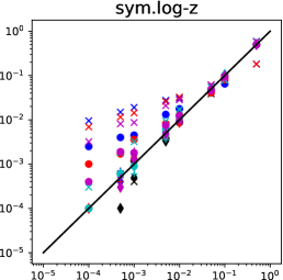 |
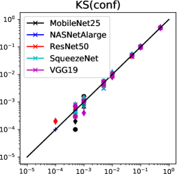
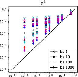
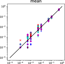
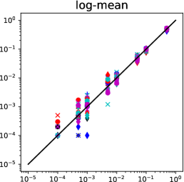
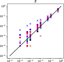
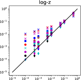
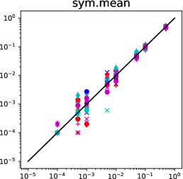
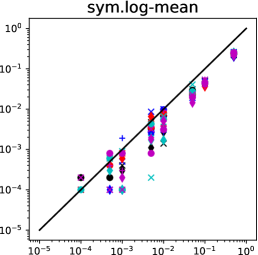
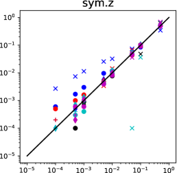
The results are depicted in Figure 2, where we report the average FPR over 10.000 random batches. One can see that KS(conf), mean and log-mean tests, as well as their symmetric counterparts, respect the FPR well. For KS(conf), this is expected, as the underlying Kolmogorov-Smirnov test has well understood statistics and universal thresholds are available. For the other four tests, the thresholds are obtained from simulating the procedure of testing on within-specs data many time. This ensures that the FPR is respected, but it requires access to the validation data any time the FPR is meant to be adapted, and it can be very time consuming, especially if small FPRs are desired.
In contrast, and - tests and their symmetric variants often produce more false positives than intended, especially for small batch sizes. This is because their thresholds are computed based on an assumption of Gaussianity, which is a good approximation only for quite large batch sizes. Finally, the label-based -test produces far too many false positives. The likely reason for this is the high dimensionality of the data: a rule of thumb says that the test is reliable when each bin of the distribution has at least 5 expected entries. This criterion is clearly violated in our situation, where the batch size is often even smaller than the number of bins. Consequently, we exclude the -test from further experiments. We keep the and - test in the list, but with the caveat that they should only be used with sufficiently large batch sizes.
In summary, of all methods, only KS(conf) achieves the two desirable properties that the FPR is respected for all batch sizes, and that adjusting the thresholds is possible efficiently and without access to validation data.
|
KS(conf) |
mean |
logmean |
|
- |
sym.mean |
sym.logmean |
sym. |
sym.- |
|
|---|---|---|---|---|---|---|---|---|---|
| AwA2-bat | 1.00 | 1.00 | 1.00 | 1.00 | 1.00 | 1.00 | 1.00 | 1.00 | 1.00 |
| AwA2-blue whale | 1.00 | 0.20 | 0.00 | 0.20 | 0.00 | 0.80 | 0.00 | 0.80 | 0.62 |
| AwA2-bobcat | 1.00 | 0.00 | 0.00 | 0.00 | 0.00 | 1.00 | 0.00 | 1.00 | 1.00 |
| AwA2-dolphin | 1.00 | 1.00 | 0.79 | 1.00 | 0.79 | 1.00 | 0.66 | 1.00 | 0.70 |
| AwA2-giraffe | 1.00 | 1.00 | 1.00 | 1.00 | 1.00 | 1.00 | 1.00 | 1.00 | 1.00 |
| AwA2-horse | 1.00 | 1.00 | 1.00 | 1.00 | 1.00 | 1.00 | 1.00 | 1.00 | 1.00 |
| AwA2-rat | 1.00 | 1.00 | 1.00 | 1.00 | 1.00 | 1.00 | 1.00 | 1.00 | 1.00 |
| AwA2-seal | 1.00 | 0.20 | 0.20 | 0.20 | 0.20 | 1.00 | 0.20 | 1.00 | 1.00 |
| AwA2-sheep | 1.00 | 0.01 | 0.00 | 0.00 | 0.00 | 0.65 | 0.00 | 0.63 | 0.82 |
| AwA2-walrus | 1.00 | 1.00 | 1.00 | 1.00 | 1.00 | 1.00 | 1.00 | 1.00 | 1.00 |
| DAVIS | 1.00 | 1.00 | 1.00 | 1.00 | 1.00 | 1.00 | 1.00 | 1.00 | 1.00 |

3.4 Results: detection rate
The true quality measure for any test is whether, at a fixed false positive rate, it is able to reliably detect changes in the input distribution. To test this, we operate the ConvNets under out-of-specs conditions by evaluating them on image data that has different characteristics than ILSVRC. Specifically, we use the 7913 images from the 10 test classes of the Animals with Attributes 2 (AwA2) (proposed split) xian2017zero . These are natural images of similar appearance as ILSVRC, but from classes that are not present in the larger dataset. Additionally, we also use the 3456 images from the 480p part of the DAVIS Perazzi2016 dataset. The images are in fact video frames and therefore exhibit different characteristics than ILSVRC’s still images, e.g. motion blur.
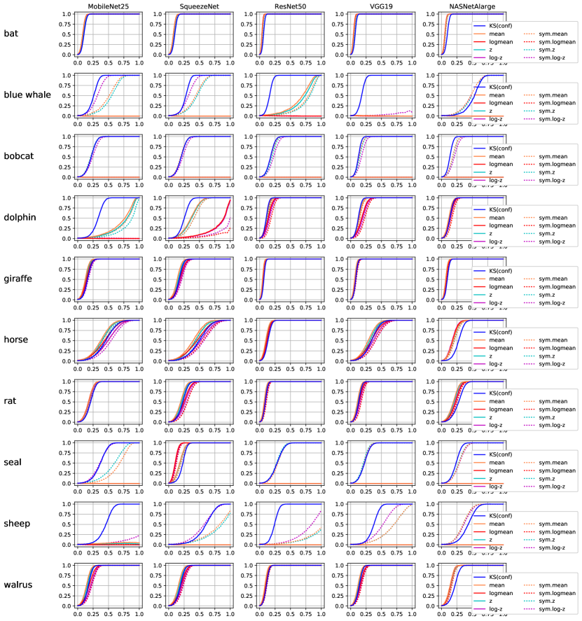
For randomly created batches, we test how often each of the tests is positive, and we report the average over 10.000 repeats. As the system is run completely out-of-specs in this scenario, all positive tests are correct, so the reported average directly corresponds to the TPR. Table 2 shows the results for an FPR and batch size averaged across the five ConvNets. More detailed results can be found in Appendix 6.
The main observation is that KS(conf) is able to reliably detect the out-of-specs behavior for all data sources, but none of the others methods are. All mean-based tests fails in at least some cases.
To shed more light on this effect, we performed more fine-grained experiments, where we create batches as mixtures of ILSVRC2012-test and AwA2 images with different mixture proportions. Figure 3 shows the results as curves of TPR versus the mixture proportion. The results fall into three characteristic classes: 1) some sources, e.g. bat, are identified reliably by all tests for all ConvNets. 2) other sources, e.g. bobcat, are identified reliably by some tests, but not at all by others. 3) for some sources, e.g. blue whale, tests show different sensitivities, i.e. some tests work only for high mixture proportions. Interestingly, the results differ substantially between networks. For example, for the ResNet50, perfect detection is typically achieved at lower mixture proportions than for MobileNet25. For NASNetAlarge on at lower mixture proportions than for MobileNet25. For NASNetAlarge on blue whale data, the symmetric mean and logmean tests work as least as well as KS(conf), but the same tests on the same data fail completely for VGG19.
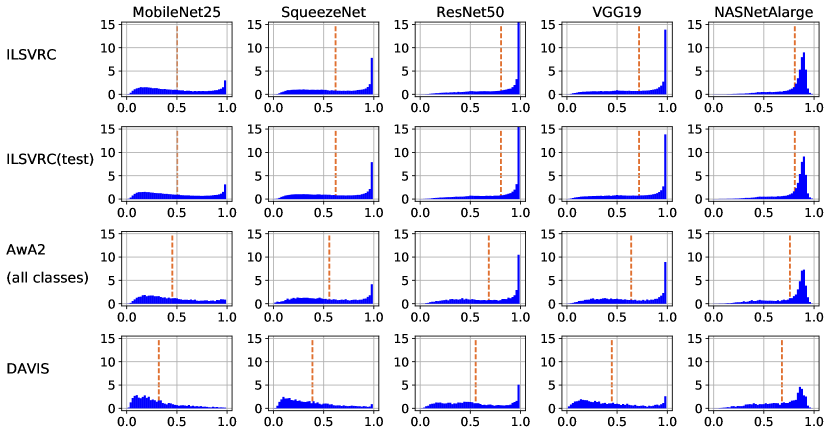
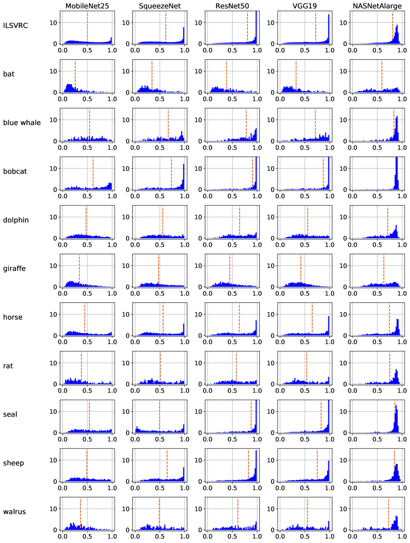
A possible source of explanation is Figure 4, where we plot the output distribution of different networks under different conditions. The first two rows reflects within-specs behavior. To some extent, they confirm the folk wisdom that ConvNet scores are biased towards high values. However, one can also see a remarkable variability between different networks. For example, MobileNet25 has a rather flat distribution compared to, e.g., VGG19, and the distribution for NASNetAlarge peaks not at but rather at . The other rows of the figure show the distribution in the same out-of-specs situations at in Figure 3, allowing to understand the reasons for the described behavior. For example, for bat, the pattern is as one would expect from an unknown class: confidences are overall much lower, which explain why the difference in distribution is easy to detect for all tests. The distribution for blue whale data differs much less from the within-specs situation, making it harder to detect. Finally, bobcat shows truly unexpected behavior: the networks are overall more confident in their predictions, which explains why in particular the single-sided mean-based tests fails in this case.
Overall, our experiments show that KS(conf) works reliably in all experimental conditions we tested. This is in agreement with the expectations from theory, as the underlying Kolmogorov-Smirnov test is known to have asymptotic power 1, meaning that if given enough data, it will detect any possible difference between distributions. In contrast to this, the mean-based tests show highly volatile behavior, which makes them unsuitable as a reliable out-of-specs test.
3.5 Results: filtering
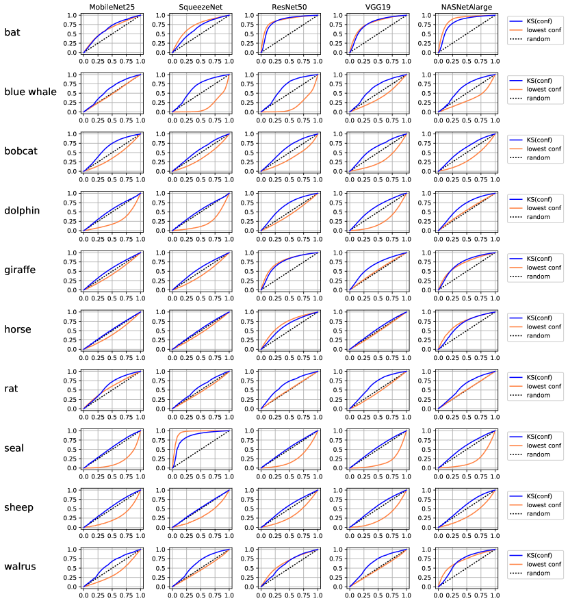
To benchmark the ability of KS(conf) to filter out images of an unexpected distribution, we run the filtering routine in the setting of the previous section, i.e. when the data at prediction time is a mixture of ILSVRC and AwA2 images. Each time KS(conf) reports a positive test, we identify a subset of images222Other subset sizes did not yield substantially different results. and measure how many of them were indeed samples from the unexpected classes. There is no established baseline for this tasks, so we compare against the intuitive baseline of reporting as subset the images with lowest confidence.
Figure 6 shows the fraction of outlier images in the identified subset for varying fractions of outlier images in the batch. A curve above the diagonal means that the test was successful in identifying suspicious images, a line below indicates that the method performs worse than a random selection. One can see that KS(conf) consistently creates better subsets than random selection would. Selecting the images of lowest confidence instead sometimes works very well (e.g. for bat), but fails in other cases (e.g. blue whale, bobcat), where it performs worse than random sampling. As can be expected, the reason lies in the fact that ConvNet confidences do not always decrease during out-of-specs operation, as we had already observed in Figure 4.
3.6 Results: camera system changes
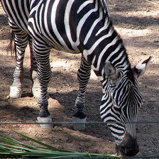
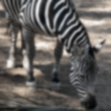
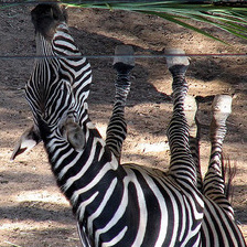
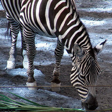
Another important reason why automatic imaging systems could operate out-of-specs is changes to the camera system. We benchmark the performance of KS(conf) to detect such, sometimes subtle, changes by running it on images that we obtain from the ILSVRC test set by applying characteristic manipulations. Because of the results of the previous section, we only report on the results of KS(conf) here. Our main goal is to gain insight into how different ConvNets react if the their inputs change due to external effect, such as incorrect camera installation, incorrect image exposure, or broken sensor pixels.
Specifically, we perform the following manipulations. Details of their implementation can be found in the corresponding sections.
-
•
loss-of-focus: we blur the image by filtering with a Gaussian kernel,
-
•
sensor noise: we add Gaussian random noise to each pixel,
-
•
dead pixels: we set a random subset of pixels to pure black or white,
-
•
wrong geometry. we flip the image horizontally or vertically, or rotate it by 90, 180 or 270 degrees
-
•
incorrect RGB/BGR color processing: we swap the and color channel,
-
•
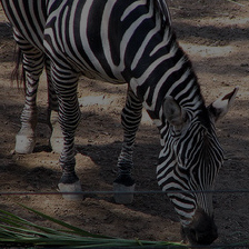
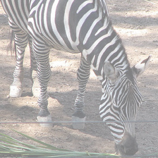
over- and under-exposure: we scale all image intensities towards or .
 |
 |
 |
 |
| original | loss-of-focus | sensor noise | dead pixels |
 |
 |
 |
 |
| wrong geometry | incorrect colors | under-exposure | over-exposure |
Figure 7 illustrates the operations. More detailed examples are provided in Appendix 7. In the following section, we discuss our main findings. A more in-depth analysis would likely find further noteworthy effects, though. Therefore, we have released the raw data and source code of the analysis for public use.333Code and data are available at https://github.com/ISTAustria-CVML/KSconf..
3.6.1 Loss of focus
To analyze the effect of a loss of focus on the ConvNet outputs, we create 100.000 perturbed test images by applying a Gaussian filter with variance , for each . Note that we filter in horizontal and vertical directions, but not across color channels.
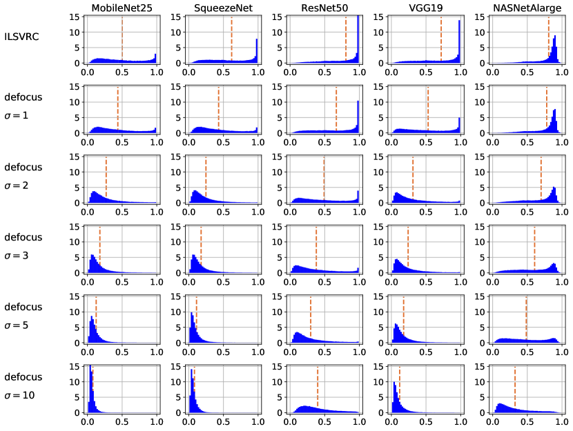
Figure 8 shows the detection rate achieved by KS(conf) for different batch sizes. Figure 9 shows the resulting distribution of confidence scores. One can see that already a rather weak loss of focus (i.e. blur) has a noticeable impact on the distribution of confidence scores. In particular, for SqueezeNet, ResNet50 and VGG19, the strong peak of confidence scores at or very close to is reduced. We observe that a loss of focus can reliably be detected from the confidence scores, and that this result seems rather stable across different ConvNet architectures.
3.6.2 Sensor Noise
To analyze the effect of sensor noise, we create 100.000 perturbed test images by adding independent Gaussian noise with variance in all color channels, for :
where generates samples from a standard Gaussian distribution and denotes the operation to clip a value to the interval .
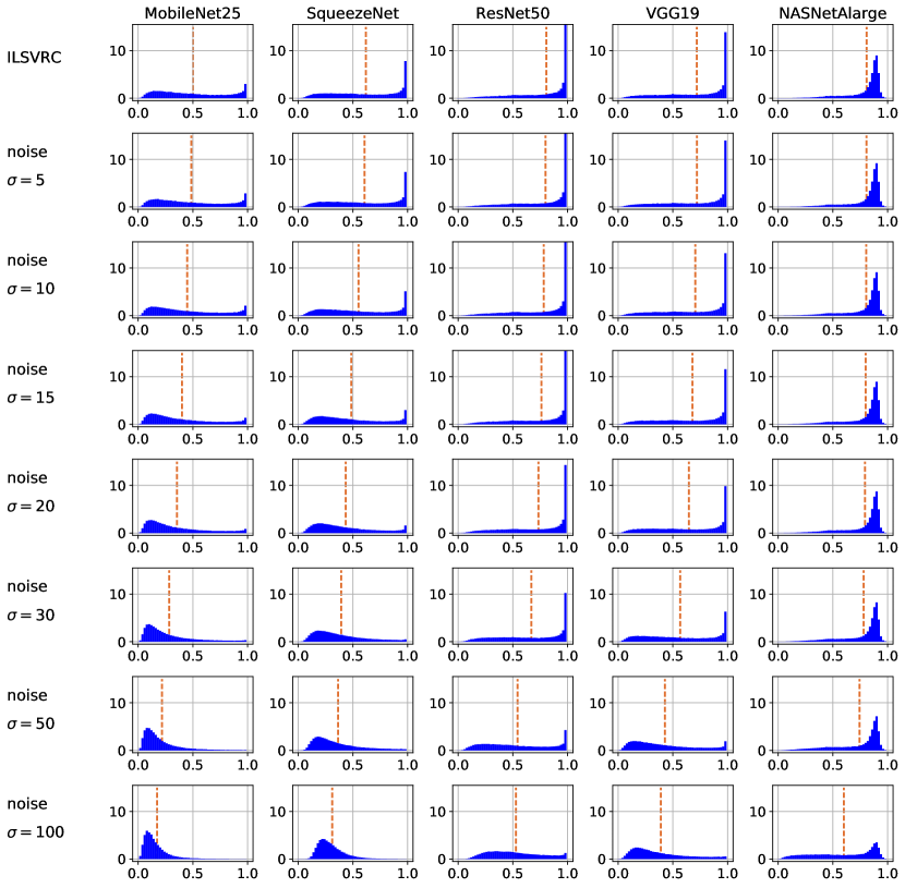
Figure 10 shows the detection rate achieved by KS(conf) for different batch sizes. Figure 11 shows the resulting distribution of confidence scores. One can see that the confidence scores of all tested ConvNets are rather robust against additive noise, especially VGG19 and NASNetAlarge for which noise of strength was not detectable, even for large batch sizes. For NASNetAlarge, even was almost undetectable from the output confidence scores. With increasing amounts of noise, however, the characteristics peaks at high confidence values start to disappear. At this level, reliable detection is possible for all ConvNet architectures.
3.6.3 Pixel Defects
We analyze the effect of cold and hot dead pixel defects by creating 100.000 perturbed test images with salt-and-pepper noise. We distort a random subset of percent of the pixels, setting half of them to pure black and half of them to pure white, for .
where and are disjoint random subsets of size each, where is the number of pixels in the image.
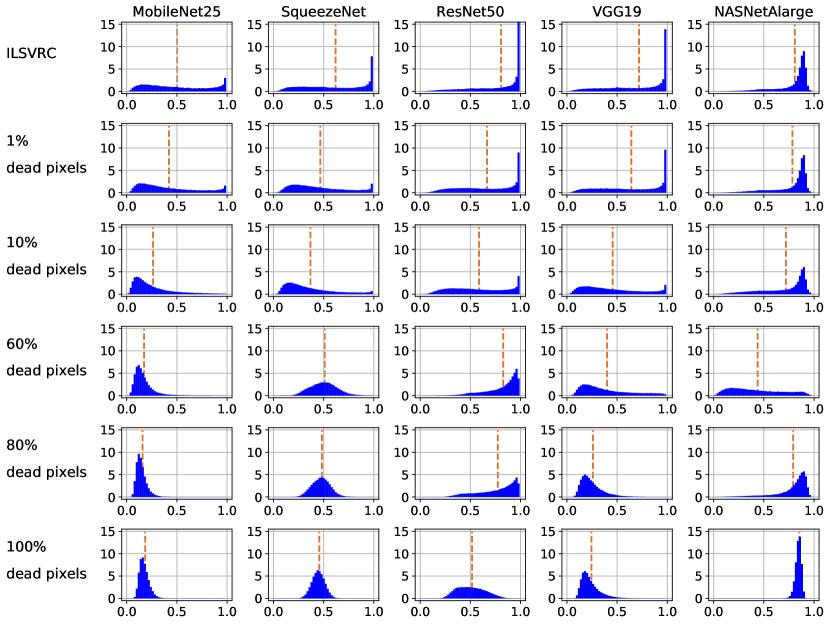
Figure 12 shows the detection rate achieved by KS(conf) for different batch sizes. Figure 13 shows the resulting distribution of confidence scores. One can see that most ConvNets are affected already by small levels of pixel defects (e.g. ). As for the previous cases, the main effect is that the distribution’s peak at high values gets reduced, until it disappears completely.
NASNetAlarge shows a very interesting and irregular behavior, though. For small perturbations (), the distribution is almost unaffected. When the perturbation strengths increases, until the expected effect happens, as the network outputs get overall less confident. For even higher perturbation strength, however, NASNetAlarge gets more confident again. For , i.e. an image consisting purely of black and white pixels in random arrangement, NASNetAlarge is overall more confidence than for the undisturbed images (it always predicts the class label window screen). We find this an important fact to keep in mind for real-world applications: one of the best existing ConvNets for image classification makes confident predictions (of wrong labels) when given random noise as input.
3.6.4 Under- and Over-Exposure
For each factor we create 100.000 perturbed test images by scaling the intensity values towards 0 (under-exposure),
| or towards 255 (over-exposure), | ||||
for .
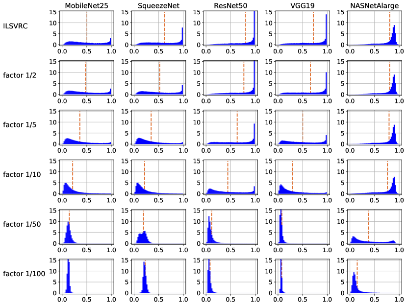
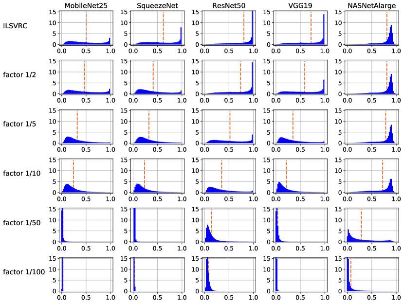
Figures 14 and 16 show the detection rate achieved by KS(conf) for different batch sizes. Figures 15 and 17 show the resulting distribution of confidence scores. One can see that the output confidences of all tested ConvNets, except for NASNetAlarge, are affected already by small levels under- or over-exposure (factor ). They react in the typical way of predicting high confidences values less frequently. NASNetAlarge tolerates a much larger amount of exposure change. A factor of is not detectable in the outputs, and a factor of only rarely. With bigger scale factors, its decisions become less confident as well, and the difference in confidence distributions can be detected reliably, as is the case for all other networks for all factors.
3.6.5 Geometry and Color Preprocessing
To simulate incorrect camera installations or geometry preprocessing, we benchmark KS(conf) with horizontally and vertically flipped images, as well as images that were rotated by 90, 180 or 270 degrees. To simulate incorrect color preprocessing, we use images in which the R and B channel have been swapped. For each transformation, we create 100.000 perturbed test images and measure KS(conf)’s detection rate.
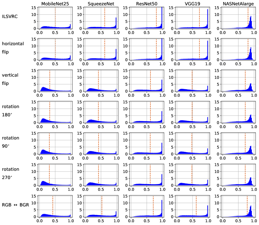
Figure 18 shows the detection rate achieved by KS(conf) for different batch sizes. Figure 19 shows the resulting distribution of confidence scores. One can see that all tested ConvNets are invariant to horizontal flips of the image, probably as an artifact of data augmentation steps that were applied during training. This could be beneficial at times, e.g. when the camera setup requires capturing images via a mirror. It could also be problematic in other situations, though, as it might make it hard to fine-tuning the networks for data that needs left-right asymmetry, such as detecting if a person is left- or right-handed. It should also be noted that it is not guaranteed that every available pretrained network exhibits near perfect invariance to horizontal flips. Therefore, when relying on it for a specific task, it should first be confirmed, e.g. using KS(conf).
Vertical flips and rotations affect the confidence distribution of all tested ConvNets, making these perturbations easily detectable. Similarly, wrong color preprocessing is also detectable from the output confidences at moderate batch sizes.
4 Conclusions
In this work, we discussed the importance of an image classifier being able to identify if it is running outside of its specifications, i.e. when the distribution of data it has to classify differs from the distribution of data it was trained for. We described a procedure, named KS(conf), based the classical statistical Kolmogorov-Smirnov test, which we apply to the distribution of the confidence values of the predicted labels. By extensive experiments we showed that KS(conf) reliably identifies out-of-specs behavior in a variety of settings, including images of unexpected classes in the data, but also effects of incorrect camera settings or sensor fatigue. We hope that our work leads to more research on how making ConvNet classifiers more trustworthy.
References
- (1) Ben-David, S., Blitzer, J., Crammer, K., Kulesza, A., Pereira, F., Vaughan, J.W.: A theory of learning from different domains. Machine Learning 79(1-2), 151–175 (2010)
- (2) Bendale, A., Boult, T.: Towards open world recognition. In: Conference on Computer Vision and Pattern Recognition (CVPR) (2015)
- (3) Dunning, T., Ertl, O.: Computing extremely accurate quantiles using t-digests. github.com (2014)
- (4) Ganin, Y., Lempitsky, V.: Unsupervised domain adaptation by backpropagation. In: International Conference on Machine Learing (ICML) (2015)
- (5) Harel, M., Mannor, S., El-Yaniv, R., Crammer, K.: Concept drift detection through resampling. In: International Conference on Machine Learing (ICML) (2014)
- (6) He, K., Zhang, X., Ren, S., Sun, J.: Deep residual learning for image recognition. In: Conference on Computer Vision and Pattern Recognition (CVPR) (2016)
- (7) Howard, A.G., Zhu, M., Chen, B., Kalenichenko, D., Wang, W., Weyand, T., Andreetto, M., Adam, H.: Mobilenets: Efficient convolutional neural networks for mobile vision applications. arXiv preprint arXiv:1704.04861 (2017)
- (8) Iandola, F.N., Han, S., Moskewicz, M.W., Ashraf, K., Dally, W.J., Keutzer, K.: SqueezeNet: AlexNet-level accuracy with 50x fewer parameters and 0.5 MB model size. arXiv preprint arXiv:1602.07360 (2016)
- (9) Jain, L.P., Scheirer, W.J., Boult, T.E.: Multi-class open set recognition using probability of inclusion. In: European Conference on Computer Vision (ECCV) (2014)
- (10) Kuncheva, L.I., Faithfull, W.J.: PCA feature extraction for change detection in multidimensional unlabeled data. IEEE Transactions on Neural Networks (T-NN) 25(1), 69–80 (2014)
- (11) Marsaglia, G., Tsang, W.W., Wang, J.: Evaluating Kolmogorov’s Distribution. Journal of Statistical Software, Articles 8(18) (2003)
- (12) Massey Jr, F.J.: The Kolmogorov-Smirnov test for goodness of fit. Journal of the American Statistical Association 46(253), 68–78 (1951)
- (13) Perazzi, F., Pont-Tuset, J., McWilliams, B., Van Gool, L., Gross, M., Sorkine-Hornung, A.: A benchmark dataset and evaluation methodology for video object segmentation. In: Conference on Computer Vision and Pattern Recognition (CVPR) (2016)
- (14) Rebuffi, S.A., Kolesnikov, A., Sperl, G., Lampert, C.H.: iCaRL: Incremental Classifier and Representation Learning. In: Conference on Computer Vision and Pattern Recognition (CVPR) (2016)
- (15) dos Reis, D.M., Flach, P., Matwin, S., Batista, G.: Fast unsupervised online drift detection using incremental Kolmogorov-Smirnov test. In: SIGKDD (2016)
- (16) Royer, A., Lampert, C.H.: Classifier adaptation at prediction time. In: Conference on Computer Vision and Pattern Recognition (CVPR) (2015)
- (17) Russakovsky, O., Deng, J., Su, H., Krause, J., Satheesh, S., Ma, S., Huang, Z., Karpathy, A., Khosla, A., Bernstein, M., Berg, A.C., Fei-Fei, L.: ImageNet Large Scale Visual Recognition Challenge. International Journal of Computer Vision (IJCV) 115(3) (2015). DOI 10.1007/s11263-015-0816-y
- (18) Sethi, T.S., Kantardzic, M., Hu, H.: A grid density based framework for classifying streaming data in the presence of concept drift. Journal of Intelligent Information Systems 46(1), 179–211 (2016)
- (19) Simonyan, K., Zisserman, A.: Very deep convolutional networks for large-scale image recognition. arXiv preprint arXiv:1409.1556 (2014)
- (20) Tange, O.: Gnu parallel - the command-line power tool. ;login: The USENIX Magazine 36(1), 42–47 (2011). URL http://www.gnu.org/s/parallel
- (21) Wang, H., Abraham, Z.: Concept drift detection for streaming data. In: International Joint Conference on Neural Networks (IJCNN) (2015)
- (22) Xian, Y., Lampert, C.H., Schiele, B., Akata, Z.: Zero-shot learning-a comprehensive evaluation of the good, the bad and the ugly. arXiv preprint arXiv:1707.00600 (2017)
- (23) Zliobaite, I.: Change with delayed labeling: When is it detectable? In: International Conference on Data Mining Workshops (2010)
- (24) Zoph, B., Vasudevan, V., Shlens, J., Le, Q.V.: Learning transferable architectures for scalable image recognition. arXiv preprint arXiv:1707.07012 (2017)
5 Appendix: Tabulated Thresholds for Kolmogorov-Smirnov Test
The following values were used as thresholds for the Kolmogorov-Smirnov test that is part of KS(conf). They were computed using the routines provided in JSSv008i18 .
| 1 | 3 | 5 | 10 | 30 | |
|---|---|---|---|---|---|
| 0.00001 | |||||
| 0.00005 | |||||
| 0.0001 | |||||
| 0.0005 | |||||
| 0.001 | |||||
| 0.005 | |||||
| 0.01 | |||||
| 0.05 | |||||
| 0.1 | |||||
| 0.5 |
| 50 | 100 | 300 | 500 | |
|---|---|---|---|---|
| 0.00001 | ||||
| 0.00005 | ||||
| 0.0001 | ||||
| 0.0005 | ||||
| 0.001 | ||||
| 0.005 | ||||
| 0.01 | ||||
| 0.05 | ||||
| 0.1 | ||||
| 0.5 |
| 3000 | 5000 | 10000 | ||
|---|---|---|---|---|
| 0.00001 | ||||
| 0.00005 | ||||
| 0.0001 | ||||
| 0.0005 | ||||
| 0.001 | ||||
| 0.005 | ||||
| 0.01 | ||||
| 0.05 | ||||
| 0.1 | ||||
| 0.5 |
6 Appendix: True Positive Rates for Different ConvNets
| MobileNet25 |
KS(conf) |
mean |
-mean |
|
-z |
sym.mean |
sym.-mean |
sym. |
sym.-z |
|---|---|---|---|---|---|---|---|---|---|
| AwA2-bat | |||||||||
| AwA2-blue whale | |||||||||
| AwA2-bobcat | |||||||||
| AwA2-dolphin | |||||||||
| AwA2-giraffe | |||||||||
| AwA2-horse | |||||||||
| AwA2-rat | |||||||||
| AwA2-seal | |||||||||
| AwA2-sheep | |||||||||
| AwA2-walrus |
| SqueezeNet | |||||||||
|---|---|---|---|---|---|---|---|---|---|
| AwA2-bat | |||||||||
| AwA2-blue whale | |||||||||
| AwA2-bobcat | |||||||||
| AwA2-dolphin | |||||||||
| AwA2-giraffe | |||||||||
| AwA2-horse | |||||||||
| AwA2-rat | |||||||||
| AwA2-seal | |||||||||
| AwA2-sheep | |||||||||
| AwA2-walrus |
| ResNet50 | |||||||||
|---|---|---|---|---|---|---|---|---|---|
| AwA2-bat | |||||||||
| AwA2-blue whale | |||||||||
| AwA2-bobcat | |||||||||
| AwA2-dolphin | |||||||||
| AwA2-giraffe | |||||||||
| AwA2-horse | |||||||||
| AwA2-rat | |||||||||
| AwA2-seal | |||||||||
| AwA2-sheep | |||||||||
| AwA2-walrus |
| VGG19 | |||||||||
|---|---|---|---|---|---|---|---|---|---|
| AwA2-bat | |||||||||
| AwA2-blue whale | |||||||||
| AwA2-bobcat | |||||||||
| AwA2-dolphin | |||||||||
| AwA2-giraffe | |||||||||
| AwA2-horse | |||||||||
| AwA2-rat | |||||||||
| AwA2-seal | |||||||||
| AwA2-sheep | |||||||||
| AwA2-walrus |
| NASNetAlarge | |||||||||
|---|---|---|---|---|---|---|---|---|---|
| AwA2-bat | |||||||||
| AwA2-blue whale | |||||||||
| AwA2-bobcat | |||||||||
| AwA2-dolphin | |||||||||
| AwA2-giraffe | |||||||||
| AwA2-horse | |||||||||
| AwA2-rat | |||||||||
| AwA2-seal | |||||||||
| AwA2-sheep | |||||||||
| AwA2-walrus |
7 Appendix: Illustrations of Synthetic Image Manipulations
7.1 Loss-of-focus (Gaussian blur)
![[Uncaptioned image]](/html/1804.04171/assets/zebra.jpg) |
![[Uncaptioned image]](/html/1804.04171/assets/zebrablur1.png) |
![[Uncaptioned image]](/html/1804.04171/assets/zebrablur2.png) |
| original | ||
![[Uncaptioned image]](/html/1804.04171/assets/zebrablur3.png) |
![[Uncaptioned image]](/html/1804.04171/assets/zebrablur4.png) |
![[Uncaptioned image]](/html/1804.04171/assets/zebrablur5.png) |
![[Uncaptioned image]](/html/1804.04171/assets/zebrablur6.png) |
![[Uncaptioned image]](/html/1804.04171/assets/zebrablur7.png) |
![[Uncaptioned image]](/html/1804.04171/assets/zebrablur8.png) |
![[Uncaptioned image]](/html/1804.04171/assets/zebrablur9.png) |
![[Uncaptioned image]](/html/1804.04171/assets/zebrablur10.png) |
|
7.2 Sensor noise (additive Gaussian noise)
![[Uncaptioned image]](/html/1804.04171/assets/zebra.jpg) |
![[Uncaptioned image]](/html/1804.04171/assets/zebranoise5.png) |
![[Uncaptioned image]](/html/1804.04171/assets/zebranoise10.png) |
| original | ||
![[Uncaptioned image]](/html/1804.04171/assets/zebranoise15.png) |
![[Uncaptioned image]](/html/1804.04171/assets/zebranoise20.png) |
![[Uncaptioned image]](/html/1804.04171/assets/zebranoise30.png) |
![[Uncaptioned image]](/html/1804.04171/assets/zebranoise50.png) |
![[Uncaptioned image]](/html/1804.04171/assets/zebranoise100.png) |
|
7.3 Pixel defects (salt-and-pepper noise)
![[Uncaptioned image]](/html/1804.04171/assets/zebra.jpg) |
![[Uncaptioned image]](/html/1804.04171/assets/zebradead1.png) |
![[Uncaptioned image]](/html/1804.04171/assets/zebradead5.png) |
| original | ||
![[Uncaptioned image]](/html/1804.04171/assets/zebradead10.png) |
![[Uncaptioned image]](/html/1804.04171/assets/zebradead20.png) |
![[Uncaptioned image]](/html/1804.04171/assets/zebradead40.png) |
![[Uncaptioned image]](/html/1804.04171/assets/zebradead60.png) |
![[Uncaptioned image]](/html/1804.04171/assets/zebradead80.png) |
![[Uncaptioned image]](/html/1804.04171/assets/zebradead100.png) |
7.4 Under-exposure (scaling towards 0)
![[Uncaptioned image]](/html/1804.04171/assets/zebra.jpg) |
![[Uncaptioned image]](/html/1804.04171/assets/zebrascale2.png) |
![[Uncaptioned image]](/html/1804.04171/assets/zebrascale3.png) |
| original | factor 1/2 | factor 1/3 |
![[Uncaptioned image]](/html/1804.04171/assets/zebrascale4.png) |
![[Uncaptioned image]](/html/1804.04171/assets/zebrascale5.png) |
![[Uncaptioned image]](/html/1804.04171/assets/zebrascale10.png) |
| factor 1/4 | factor 1/5 | factor 1/10 |
![[Uncaptioned image]](/html/1804.04171/assets/zebrascale20.png) |
![[Uncaptioned image]](/html/1804.04171/assets/zebrascale50.png) |
![[Uncaptioned image]](/html/1804.04171/assets/zebrascale100.png) |
| factor 1/20 | factor 1/50 | factor 1/100 |
7.5 Over-exposure (scaling towards 255)
![[Uncaptioned image]](/html/1804.04171/assets/zebra.jpg) |
![[Uncaptioned image]](/html/1804.04171/assets/zebrascale-2.png) |
![[Uncaptioned image]](/html/1804.04171/assets/zebrascale-3.png) |
| original | factor 1/2 | factor 1/3 |
![[Uncaptioned image]](/html/1804.04171/assets/zebrascale-4.png) |
![[Uncaptioned image]](/html/1804.04171/assets/zebrascale-5.png) |
![[Uncaptioned image]](/html/1804.04171/assets/zebrascale-10.png) |
| factor 1/4 | factor 1/5 | factor 1/10 |
![[Uncaptioned image]](/html/1804.04171/assets/zebrascale-20.png) |
![[Uncaptioned image]](/html/1804.04171/assets/zebrascale-50.png) |
![[Uncaptioned image]](/html/1804.04171/assets/zebrascale-100.png) |
| factor 1/20 | factor 1/50 | factor 1/100 |
7.6 Wrong geometry and color preprocessing
![[Uncaptioned image]](/html/1804.04171/assets/zebra.jpg) |
![[Uncaptioned image]](/html/1804.04171/assets/zebraflip2.png) |
![[Uncaptioned image]](/html/1804.04171/assets/zebraflip3.png) |
| original | horizontal flip | vertical flip |
![[Uncaptioned image]](/html/1804.04171/assets/zebraflip4.png) |
![[Uncaptioned image]](/html/1804.04171/assets/zebraflip5.png) |
![[Uncaptioned image]](/html/1804.04171/assets/zebraflip6.png) |
| 180∘ rotation | 90∘ rotation | 270∘ rotation |
![[Uncaptioned image]](/html/1804.04171/assets/zebraBGR.png) |
||
| RGB BGR |