Exploring deep learning as an event classification method for the Cherenkov Telescope Array

Abstract:

Telescopes based on the imaging atmospheric Cherenkov technique (IACTs) detect images of the atmospheric showers generated by gamma rays and cosmic rays as they are absorbed by the atmosphere. The much more frequent cosmic-ray events form the main background when looking for gamma-ray sources, and therefore IACT sensitivity is significantly driven by the capability to distinguish between these two types of events. Supervised learning algorithms, like random forests and boosted decision trees, have been shown to effectively classify IACT events. In this contribution we present results from exploratory work using deep learning as an event classification method for the Cherenkov Telescope Array (CTA). CTA, conceived as an array of tens of IACTs, is an international project for a next-generation ground-based gamma-ray observatory, aiming to improve on the sensitivity of current-generation experiments by an order of magnitude and provide energy coverage from 20 GeV to more than 300 TeV.

1 Introduction

In this contribution we present an exploratory work on the application of deep learning methods to the problem of event classification for imaging atmospheric Cherenkov telescopes (IACTs). IACTs are capable of imaging the particle showers created in the atmosphere by high energy ($\gtrsim 10$’s GeV) gamma rays. By focusing the Cherenkov photons emitted by the charged particles in the shower onto a high-sensitivity camera, images of the showers can be obtained. However, gamma-ray initiated showers are a minor fraction of the total number of observed atmospheric showers, which is dominated by a background of cosmic ray-induced showers. The ability to discriminate between gamma-ray events and cosmic-ray events is one of the major factors determining the sensitivity of IACTs to astrophysical gamma-ray sources.

Gamma-ray initiated showers are driven by purely electromagnetic processes, while cosmic-ray showers add hadronic processes to the former. This difference expresses itself in the morphology of the imaged shower and can be exploited to discriminate between the two cases. Originally, IACT images were parametrized in terms of their second moments [1], and event classification was performed by applying box cuts in the corresponding parameter space. Current generation IACTs have satisfactorily implemented classification schemes based on supervised learning algorithms trained on a set of event-level parameters reconstructed from multiple telescope images, as is the case of the random forest for the MAGIC telescope [2], and boosted decision trees (BDT) for the VERITAS telescope [3] and the H.E.S.S. telescope [4, 5], which have substantially improved their sensitivity.

Presently, deep convolutional neural networks (CNNs), also known as deep learning (DL), is the leading approach to supervised representation learning, encompassing the problem of image classification [6]. Due to its flexibility, versatility, and performance, DL has been applied to the analysis of data from diverse scientific disciplines, including high energy physics (see, e.g., [7, 8]). Thus, it is natural to ask whether IACT image classification could benefit from this approach, and efforts have begun to give an answer [9]. One of the main advantages of DL against previous machine learning approaches to IACT image classification is that CNNs do not need the images to be parametrized, and therefore have access to all the information contained in them, opening the way to exploiting image features that might get lost or washed out during the parametrization.

In this work, we investigate DL as an event classification method for the future Cherenkov Telescope Array (CTA,[10]). CTA is an international project aimed at constructing the next-generation IACT observatory, with an order of magnitude greater sensitivity than current-generation experiments. CTA will consist of two installations, one located in the Northern hemisphere (La Palma, Spain) and another in the Southern hemisphere (Cerro Paranal, Chile), each one equipped with an array of few tens of IACTs of different sizes optimized to different energy bands ranging from 20 GeV to more than 300 TeV. For this work we use images from Monte Carlo simulated events as detected by an array of 9.7-m-aperture Schwarzschild-Couder medium-sized telescopes (SC-MST, [11]) to train several known DL architectures in the event discrimination task, leaving the consideration of other telescope models to future works. Additionally, we focus on single-image classification as opposed to event-level classification (using multiple images from a same event to take advantage of stereoscopic information), which will be dealt with in subsequent works. Thus, this study serves as a proof of principle that CNNs are capable of classifying air shower images, and the resulting single-image networks will serve as a useful first stage of the more complex array-level networks we plan to later implement.

2 Deep learning

Deep convolutional neural networks (CNNs) operate fundamentally like traditional fully connected networks, but with innovations including local receptive fields, shared weights, and pooling that significantly reduce the parameter count and computational cost. A CNN consists of many layers, each containing a set of nodes. In the input layer, each node corresponds to one image pixel. In the following convolutional layers, each node receives inputs from a small number of nodes in the previous layer forming its local receptive field. These inputs are convolved with several ”filters”, consisting of a grid of weights spanning the receptive field, to produce the activations. The filter weights are shared across each layer’s nodes, a design choice that reflects the translational and rotational invariance of many visual features. A nonlinear activation function such as rectified linear unit is then applied to give the node output. We refer the reader to [12] for a concise overview of DL and to [6] for a more detailed work on the subject.

In some architectures, convolutional layers alternate with pooling layers that combine information from neighboring nodes to reduce the dimensionality of the feature maps and incorporate information from wider areas of the original image  [12]. This structure reflects the localized nature of image features, dramatically reducing the needed weight parameters by ignoring dependencies between distant pixels until later layers.

The last layer of a classifier outputs a prediction which is compared to the true label using a loss function, such as binary cross-entropy for binary classification. The network learns using backpropagation: gradients of the loss surface in high-dimensional weight space are calculated and the weights updated in the direction that minimizes the loss using a variant of gradient descent. Training is done in batches such that, for each epoch, the weights are updated based on the gradient from one sample at a time, repeated until the network has seen the entire training set.

3 Application to CTA event images

We used the Monte Carlo simulation chain for CTA described in [13], where the atmospheric showers are simulated with Corsika [14] and the telescope optics and camera readout are simulated with Sim_telarray [15]. We simulated the response of an array of 8 SCTs to $\sim 5\times 10^{9}$ proton showers and $\sim 9\times 10^{8}$ gamma-ray showers, assuming an altitude and atmospheric profile describing the conditions in the Roque de los Muchachos Observatory (La Palma, Spain), where the Northern installation of the CTA Observatory will be located. The SCT model, by design, combines an excellent point spread function across a wide field of view with a camera featuring the highest number of pixels among CTA telescopes. SCTs will potentially provide CTA with its highest-resolution shower images, thus motivating the selection of SCT images for this study. In addition, SCT gamma-ray cameras feature square pixels, as opposed to other types of CTA telescope models whose cameras are composed of hexagonal pixels, avoiding the need of transforming the hexagonal lattices into 2D arrays, the common input format for CNNs.

Figure 1: Some sample images from our data set, corresponding to independent events. Left image from a gamma-ray initiated shower. Right: image from proton initiated shower. The images have been normalized for better visualization.

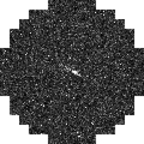
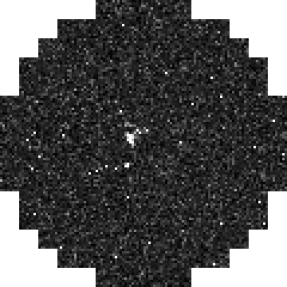
The energy distribution of the initial particles ranged from 3 GeV to 330 TeV in the case of gamma rays and 4 GeV to 600 TeV in the case of protons. The arrival direction of both particle types was homogeneously distributed inside a cone of 10^∘ radius with axis co-linear with the pointing position of the telescopes. Two different pointing positions were chosen, sharing a zenith angle of 20^∘ and Azimuth angle of 0^∘ and 180^∘, splitting the simulated events evenly between the two. The output of Sim_telarray consists of the collection of digitized photodetector pulses, for each triggered telescope camera, on an event-by-event basis. We used the IACT analysis package Event Display to convert Sim_telarray files into ROOT format. In order to convert the raw data in ROOT format into shower images we developed the code ImageExtractor, based on ROOT and the OpenCV library. ImageExtractor performs a simple pulse integration and stores the integrated pulse, in digital counts, into a 120x120 array representing the camera topology that is eventually saved into a 16-bit depth portable network graphics (PNG) image. Relevant Monte Carlo parameters, including the particle type, particle energy, impact parameter, and triggered telescope number, are stored in the image header for further reference.

Cut

Offset $\leq 3^{\circ}$

$-2<MSCW<2$

$-2<MSCL<5$

$EChi2S\geq 0$

$ERecS>0$ TeV

$0$ km $<$ Emission height $<50$ km

$dES\geq 0$ TeV

Table 1: Arrival direction and sanity cuts applied to all data. Only events passing all cuts were used for training, validation, or testing. The cut variables are: Offset between camera center and MC arrival direction of the event; MSCW (MSCL) is the event’s mean scaled width (length); EChi2S is the $\chi^{2}$ its estimated vs. reconstructed energy value; ERecS (Emission height) is its reconstructed energy (emission height); dES is the reconstructed energy error.

Several cuts were applied to the data before training. For all events, the arrival direction of the shower was constrained to offsets between $0^{\circ}$ and $3^{\circ}$ and the event telescope multiplicity was required to be $\geq 3$. Sanity cuts were also applied on several reconstructed event parameters (see Table 1). These cuts were chosen to match those in one of the standard CTA analysis chains, Eventdisplay, in particular to train the default BDT-based image classification [3] and use the classification performance achieved by the BDTs as a reference. The data were separated into three energy bins corresponding to low, medium, and high energies (see Table 2). Training was performed separately on each energy bin.

Within each bin, the data were randomly split into training, validation, and test sets, comprising 80%, 10%, and 10% of each bin’s data. Only images in the training sets were used as inputs for the CNN, while those in the validation sets were used to measure the network’s performance after each epoch of training. The images in the test sets were reserved to obtain a final measure of the network’s accuracy after training was complete. To instantiate our models, we used the high-level neural network library Keras [16] with Theano  [17] as the computational back-end. For this work we explored two well-known models, ResNet50 [18] and Inception V3 [19], both available as applications within Keras. Inception V3, by using batch normalization, optimization of layer dimensions, careful balancing of network width and depth, and aggressive factorizations of the convolutional layers, is able to achieve state of the art performance on the ILSVRC 2012 benchmark. ResNet50, developed in parallel to Inception V3, takes a different approach by using residual mapping (implemented as ”shortcut” connections across convolutional layers) to more effectively train very deep networks. Using this approach, networks of over 100 layers have been successfully trained to very high accuracies.

Energy	$E_{min}$	$E_{max}$	$N_{gamma}$	$N_{proton}$
bin	[TeV]	[TeV]
Total			4160578	4056723
Low	0.1	0.31	727316	228959
Medium	0.31	1	657397	119704
High	1	10	642034	72034

Table 2: Dataset used in this proceeding. All data were simulated at a Zenith angle of $20^{\circ}$ and at an Azimuth angle of either $0^{\circ}$ or $180^{\circ}$, split roughly evenly between the two. Total statistics are prior to any cut.

We trained both architectures on our dataset and compared their performance. The networks were not initialized with any pretrained weights. To adapt the networks for CTA data, the input images were resized to 240 x 240 arrays and the output layer replaced with a binary classifier. Training was conducted on two different computing systems sharing identical datasets and featuring similarly performing GPUs: a Nvidia™ GeForce GTX TITAN X Pascal and Nvidia™ GeForce GTX 1080 Ti. The training time over the full dataset was of 12 hours per energy bin and per model, while the classification of data is performed approximately three orders of magnitude faster.

4 Results

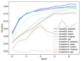
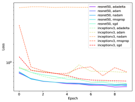
The maximum accuracy achievable by training a given network depends on the backpropagation algorithm used. We surveyed a subset of optimizers directly available in Keras in order to identify the best performing ones in terms of accuracy (fraction of images showing a classifier score for its true category higher than 0.5, where the classifier range is 0 to 1). Tests were conducted using stochastic gradient descent (SGD), RMSprop, Adam, Adadelta, and Nadam optimizers [20]. We trained ResNet50 and Inception V3 on a small subset of images ($2\times 10^{5}$ images per category), for a duration of 10 epochs, to evaluate the model accuracy and loss as a function of the chosen optimizer. We did not optimize the learning rates or any other hyperparameters of the different optimizers, adopting the default values as provided in Keras. Our findings are shown in Fig. 2. Our results show that the default hyperparameters work reasonably well for ResNet50 while most optimizers are not well tuned for Inception V3. Adadelta provided the highest accuracies at epoch 10 for both models. Consequently, we adopted Adadelta as the optimizer for the training on the full data set, allowing for a more direct comparison between performances.

After the selection of the optimizer, both ResNet50 and Inception V3 networks were trained using the full training and validation sets for the three energy bins. We trained our models for 10 epochs, which appeared to be enough for a stabilization of the training accuracy without a drop in the validation accuracy that might point out overtraining. A summary of the evolution of training and validation accuracy as well as loss can be found in Fig. 3. We found that both models achieve a very similar training accuracy at epoch 10, ResNet50 learning at a slightly faster pace than Inception V3, with the latter providing with marginally higher validation accuracies in the low ($0.3\%$) and high ($0.4\%$) energy ranges, while tying in the medium energy range. As expected, higher energies provide with higher accuracies, since the images tend to be larger and brighter (more information), thus allowing for a more effective training. A summary of the highest validation accuracies per training can be found in Table 3.

Figure 2: Network accuracy (left) and loss (right) as a function of the training epoch, for ResNet50 and InceptionV3 models. The training was performed on a subset of $2\times 10^{5}$ images per category drawn from the medium energy bin of the training dataset.

Model	Low E.	Med. E.	High E.
ResNet50	81.1%	90.1%	91.2%
Inception V3	81.4%	90.1%	91.6%

Table 3: Highest classification accuracy on the validation data set for ResNet50 and Inception V3 models for all energy bins.

Figure 3: Network training accuracy (right) and loss (left) as a function of the training epoch, for ResNet50 and InceptionV3 models and all three energy bins. For each model and energy bin both the training and validation accuracy and loss are shown (upper plot), as well as the gap between the two (lower plot): training curves are represented by thick lines, while validation accuracy curves are represented by thin lines. The training was performed on our full data set, independently for each energy bin.

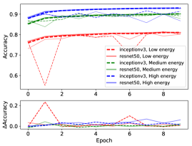
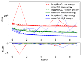
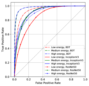
We generated receiver operating characteristic (ROC) curves for all scenarios by passing the corresponding test subsets to the trained models showing the highest validation accuracies. The collection of all ROC curves can be found in Fig. 4. It can be seen that, for the low and medium energies, both models are performing almost equally. For the highest energies there seems to be some distance between InceptionV3 and ResNet50 that we suspect may be originated by a higher susceptibility of the former to the relatively low image statistics present in the proton subsample, which is hinted in the behavior of the validation and loss for the validation sample in Fig. 3. Similarly found in the behavior of the BDTs, the InceptionV3 ROC curves for medium and high energies are close together, although we suspect that the discrimination power of CNNs in the highest energy range may increase if a larger sample of proton images is used for the training of the CNNs. While the ROC curves from the tested CNN architectures are significantly below the corresponding ones for the BDT-based classification method, one must bear in mind that the latter draws its power from a multi-image event stereo reconstruction, whereas our models are trained on individual images (coming from events that survive the above mentioned cuts but lacking any additional stereo information). Thus, the BDT ROC curve should be seen as a reference, a target to overtake in the future.

5 Conclusion and outlook

We have demonstrated that DL is capable of classifying simulated IACT images, here represented by SCT images, without any prior parametrization nor any assumption on the nature of the images themselves. The accuracy of the tested models is energy dependent, ranging from  81.4% in the low energy range to 91.6% in the high energy range for the Inception V3 architecture.

Figure 4: ROC curves from test data classified with ResNet50 and Inception V3 for the low, medium, and high energy bins. As a reference we show the ROC curves corresponding to BDT trained on the same data set (events parametrized using stereo information).

After applying CNNs to gamma-hadron separation on single-telescope images, the next step is to apply these techniques to array-level classification. IACT array analysis methods rely on combining information from multiple telescopes to achieve high-quality stereo shower reconstruction, perform background discrimination, and calculate reconstructed parameters. Going forward, the focus of our efforts will be on developing multi-input architectures consisting of separate CNNs for each telescope, which will then combine information through a fully-connected classifier to achieve more effective gamma-hadron separation on the array level. Eventually, we will assess the benefits of DL as compared to the current standard analysis on the instrument response functions.

We also plan to further investigate different architectures, gradient descent algorithms, and other hyper-parameters, narrowing down on the choice that provides optimal results. It may be possible to achieve superior results by customizing networks for the specific task of Cherenkov image classification. Other promising applications for CNNs to IACT data analysis include using similar methods to those presented here to do energy and angular reconstruction and performing more difficult background discrimination tasks such as gamma/electron separation or cosmic-ray composition studies.

6 Acknowledgments

We gratefully acknowledge support from the agencies and organizations listed under Funding Agencies at this website: http://www.cta-observatory.org/. This work was conducted in the context of the Analysis and Simulations Working Group of the CTA Consortium. DN wants to acknowledge support from the Spanish Ministry of Economy, Industry, and Competitiveness / ERDF UE grant FPA2015-73913-JIN. We want to thank Tarek Hassan for discussions at the early stages of this work. We acknowledge the support of NVIDIA Corporation with the donation of the Titan X Pascal GPU used for this research.

References

- [1] A. M. Hillas, Cerenkov light images of EAS produced by primary gamma, International Cosmic Ray Conference 3 (Aug., 1985).
- [2] J. Albert et al., Implementation of the Random Forest method for the Imaging Atmospheric Cherenkov Telescope MAGIC, Nuclear Instruments and Methods in Physics Research A 588 (Apr., 2008) 424–432, [arXiv:0709.3719].
- [3] M. Krause, E. Pueschel, and G. Maier, Improved /hadron separation for the detection of faint -ray sources using boosted decision trees, Astroparticle Physics 89 (2017) 1–9.
- [4] S. Ohm, C. van Eldik, and K. Egberts, /hadron separation in very-high-energy -ray astronomy using a multivariate analysis method, Astroparticle Physics 31 (June, 2009) 383–391, [arXiv:0904.1136].
- [5] Y. Becherini, A. Djannati-Ataï, V. Marandon, M. Punch, and S. Pita, A new analysis strategy for detection of faint -ray sources with Imaging Atmospheric Cherenkov Telescopes, Astroparticle Physics 34 (July, 2011) 858–870, [arXiv:1104.5359].
- [6] I. Goodfellow, Y. Bengio, and A. Courville, Deep Learning. MIT Press, 2016. http://www.deeplearningbook.org.
- [7] P. Baldi, P. Sadowski, and D. Whiteson, Searching for Exotic Particles in High-Energy Physics with Deep Learning, Nature Commun. 5 (2014) 4308, [arXiv:1402.4735].
- [8] A. Aurisano, A. Radovic, D. Rocco, A. Himmel, M. D. Messier, E. Niner, G. Pawloski, F. Psihas, A. Sousa, and P. Vahle, A convolutional neural network neutrino event classifier, Journal of Instrumentation 11 (Sept., 2016) P09001, [arXiv:1604.01444].
- [9] Q. Feng and T. T. Y. Lin, The analysis of VERITAS muon images using convolutional neural networks, ArXiv e-prints (Nov., 2016) [arXiv:1611.09832].
- [10] B. S. Acharya et al., Introducing the CTA concept, Astroparticle Physics 43 (Mar., 2013) 3–18.
- [11] V. Vassiliev, S. Fegan, and P. Brousseau, Wide field aplanatic two-mirror telescopes for ground-based -ray astronomy, Astroparticle Physics 28 (Sept., 2007) 10–27, [astro-ph/0612718].
- [12] Y. LeCun, Y. Bengio, and G. Hinton, Deep learning, Nature 521 (2015), no. 7553 436–444.
- [13] K. Bernlöhr and CTA Consortium, Monte Carlo design studies for the Cherenkov Telescope Array, Astroparticle Physics 43 (Mar., 2013) 171–188, [arXiv:1210.3503].
- [14] D. Heck, J. Knapp, J. N. Capdevielle, G. Schatz, and T. Thouw, CORSIKA: a Monte Carlo code to simulate extensive air showers. Feb., 1998.
- [15] K. Bernlöhr, Simulation of imaging atmospheric Cherenkov telescopes with CORSIKA and sim_ telarray, Astroparticle Physics 30 (Oct., 2008) 149–158, [arXiv:0808.2253].
- [16] F. Chollet et al., “Keras.” https://github.com/fchollet/keras, 2015.
- [17] Theano Development Team, Theano: A Python framework for fast computation of mathematical expressions, (May, 2016) [arXiv:1605.02688].
- [18] K. He, X. Zhang, S. Ren, and J. Sun, Deep Residual Learning for Image Recognition, ArXiv e-prints (Dec., 2015) [arXiv:1512.03385].
- [19] C. Szegedy, V. Vanhoucke, S. Ioffe, J. Shlens, and Z. Wojna, Rethinking the Inception Architecture for Computer Vision, ArXiv e-prints (Dec., 2015) [arXiv:1512.00567].
- [20] I. Sutskever, J. Martens, G. Dahl, and G. Hinton, On the importance of initialization and momentum in deep learning, in International conference on machine learning, pp. 1139–1147, 2013.