Fisher GAN

Youssef Mroueh, Tom Sercu
mroueh@us.ibm.com, tom.sercu1@ibm.com
* Equal Contribution
AI Foundations, IBM Research AI
IBM T.J Watson Research Center
Abstract

Generative Adversarial Networks (GANs) are powerful models for learning complex distributions. Stable training of GANs has been addressed in many recent works which explore different metrics between distributions. In this paper we introduce Fisher GAN which fits within the Integral Probability Metrics (IPM) framework for training GANs. Fisher GAN defines a critic with a data dependent constraint on its second order moments. We show in this paper that Fisher GAN allows for stable and time efficient training that does not compromise the capacity of the critic, and does not need data independent constraints such as weight clipping. We analyze our Fisher IPM theoretically and provide an algorithm based on Augmented Lagrangian for Fisher GAN. We validate our claims on both image sample generation and semi-supervised classification using Fisher GAN.

1 Introduction

Generative Adversarial Networks (GANs) [1] have recently become a prominent method to learn high-dimensional probability distributions. The basic framework consists of a generator neural network which learns to generate samples which approximate the distribution, while the discriminator measures the distance between the real data distribution, and this learned distribution that is referred to as fake distribution. The generator uses the gradients from the discriminator to minimize the distance with the real data distribution. The distance between these distributions was the object of study in [2], and highlighted the impact of the distance choice on the stability of the optimization. The original GAN formulation optimizes the Jensen-Shannon divergence, while later work generalized this to optimize f-divergences [3], KL [4], the Least Squares objective [5]. Closely related to our work, Wasserstein GAN (WGAN) [6] uses the earth mover distance, for which the discriminator function class needs to be constrained to be Lipschitz. To impose this Lipschitz constraint, WGAN proposes to use weight clipping, i.e. a data independent constraint, but this comes at the cost of reducing the capacity of the critic and high sensitivity to the choice of the clipping hyper-parameter. A recent development Improved Wasserstein GAN (WGAN-GP) [7] introduced a data dependent constraint namely a gradient penalty to enforce the Lipschitz constraint on the critic, which does not compromise the capacity of the critic but comes at a high computational cost.

We build in this work on the Integral probability Metrics (IPM) framework for learning GAN of [8]. Intuitively the IPM defines a critic function f𝑓f, that maximally discriminates between the real and fake distributions. We propose a theoretically sound and time efficient data dependent constraint on the critic of Wasserstein GAN, that allows a stable training of GAN and does not compromise the capacity of the critic. Where WGAN-GP uses a penalty on the gradients of the critic, Fisher GAN imposes a constraint on the second order moments of the critic. This extension to the IPM framework is inspired by the Fisher Discriminant Analysis method.

The main contributions of our paper are:

  1. 1.

    We introduce in Section 2 the Fisher IPM, a scaling invariant distance between distributions. Fisher IPM introduces a data dependent constraint on the second order moments of the critic that discriminates between the two distributions. Such a constraint ensures the boundedness of the metric and the critic. We show in Section 2.2 that Fisher IPM when approximated with neural networks, corresponds to a discrepancy between whitened mean feature embeddings of the distributions. In other words a mean feature discrepancy that is measured with a Mahalanobis distance in the space computed by the neural network.

  2. 2.

    We show in Section 3 that Fisher IPM corresponds to the Chi-squared distance (χ2subscript𝜒2\chi_{2}) when the critic has unlimited capacity (the critic belongs to a universal hypothesis function class). Moreover we prove in Theorem 2 that even when the critic is parametrized by a neural network, it approximates the χ2subscript𝜒2\chi_{2} distance with a factor which is a inner product between optimal and neural network critic. We finally derive generalization bounds of the learned critic from samples from the two distributions, assessing the statistical error and its convergence to the Chi-squared distance from finite sample size.

  3. 3.

    We use Fisher IPM as a GAN objective 111Code is available at https://github.com/tomsercu/FisherGAN and formulate an algorithm that combines desirable properties (Table 1): a stable and meaningful loss between distributions for GAN as in Wasserstein GAN [6], at a low computational cost similar to simple weight clipping, while not compromising the capacity of the critic via a data dependent constraint but at a much lower computational cost than [7]. Fisher GAN achieves strong semi-supervised learning results without need of batch normalization in the critic.

Table 1: Comparison between Fisher GAN and recent related approaches.
Stability Unconstrained Efficient Representation
capacity Computation power (SSL)
Standard GAN [1, 9]              ✓       ✓       ✓
WGAN, McGan [6, 8]       ✓              ✓       
WGAN-GP [7]       ✓       ✓              ?
Fisher Gan (Ours)       ✓       ✓       ✓       ✓

2 Learning GANs with Fisher IPM

2.1 Fisher IPM in an arbitrary function space: General framework

Integral Probability Metric (IPM). Intuitively an IPM defines a critic function f𝑓f belonging to a function class \mathscr{F}, that maximally discriminates between two distributions. The function class \mathscr{F} defines how f𝑓f is bounded, which is crucial to define the metric. More formally, consider a compact space XX\pazocal{X} in dsuperscript𝑑\mathbb{R}^{d}. Let \mathscr{F} be a set of measurable, symmetric and bounded real valued functions on XX\pazocal{X}. Let 𝒫(X)𝒫X\mathscr{P}(\pazocal{X}) be the set of measurable probability distributions on XX\pazocal{X}. Given two probability distributions ,𝒫(X)𝒫X\mathbb{P},\mathbb{Q}\in\mathscr{P}({\pazocal{X}}), the IPM indexed by a symmetric function space \mathscr{F} is defined as follows [10]:

d(,)=supf{𝔼xf(x)𝔼xf(x)}.subscript𝑑subscriptsupremum𝑓similar-to𝑥𝔼𝑓𝑥similar-to𝑥𝔼𝑓𝑥d_{\mathscr{F}}(\mathbb{P},\mathbb{Q})=\sup_{f\in\mathscr{F}}\Big{\{}\underset{x\sim\mathbb{P}}{\mathbb{E}}f(x)-\underset{x\sim\mathbb{Q}}{\mathbb{E}}f(x)\Big{\}}. (1)

It is easy to see that dsubscript𝑑d_{\mathscr{F}} defines a pseudo-metric over 𝒫(X)𝒫X\mathscr{P}(\pazocal{X}). Note specifically that if \mathscr{F} is not bounded, supfsubscriptsupremum𝑓\sup_{f} will scale f𝑓f to be arbitrarily large. By choosing \mathscr{F} appropriately [11], various distances between probability measures can be defined.

First formulation: Rayleigh Quotient. In order to define an IPM in the GAN context, [6, 8] impose the boundedness of the function space via a data independent constraint. This was achieved via restricting the norms of the weights parametrizing the function space to a psubscript𝑝\ell_{p} ball. Imposing such a data independent constraint makes the training highly dependent on the constraint hyper-parameters and restricts the capacity of the learned network, limiting the usability of the learned critic in a semi-supervised learning task. Here we take a different angle and design the IPM to be scaling invariant as a Rayleigh quotient. Instead of measuring the discrepancy between means as in Equation (1), we measure a standardized discrepancy, so that the distance is bounded by construction. Standardizing this discrepancy introduces as we will see a data dependent constraint, that controls the growth of the weights of the critic f𝑓f and ensures the stability of the training while maintaining the capacity of the critic. Given two distributions ,𝒫(X)𝒫X\mathbb{P},\mathbb{Q}\in\mathscr{P}(\pazocal{X}) the Fisher IPM for a function space \mathscr{F} is defined as follows:

d(,)=supf𝔼x[f(x)]𝔼x[f(x)]1/2𝔼xf2(x)+1/2𝔼xf2(x).subscript𝑑subscriptsupremum𝑓similar-to𝑥𝔼delimited-[]𝑓𝑥similar-to𝑥𝔼delimited-[]𝑓𝑥12subscript𝔼similar-to𝑥superscript𝑓2𝑥12subscript𝔼similar-to𝑥superscript𝑓2𝑥d_{\mathscr{F}}(\mathbb{P},\mathbb{Q})=\sup_{f\in\mathscr{F}}\frac{\underset{x\sim\mathbb{P}}{\mathbb{E}}[f(x)]-\underset{x\sim\mathbb{Q}}{\mathbb{E}}[f(x)]}{\sqrt{\nicefrac{{1}}{{2}}\mathbb{E}_{x\sim\mathbb{P}}f^{2}(x)+\nicefrac{{1}}{{2}}\mathbb{E}_{x\sim\mathbb{Q}}f^{2}(x)}}. (2)

While a standard IPM (Equation (1)) maximizes the discrepancy between the means of a function under two different distributions, Fisher IPM looks for critic f𝑓f that achieves a tradeoff between maximizing the discrepancy between the means under the two distributions (between class variance), and reducing the pooled second order moment (an upper bound on the intra-class variance).

Standardized discrepancies have a long history in statistics and the so-called two-samples hypothesis testing. For example the classic two samples Student’s tlimit-from𝑡t- test defines the student statistics as the ratio between means discrepancy and the sum of standard deviations. It is now well established that learning generative models has its roots in the two-samples hypothesis testing problem [12]. Non parametric two samples testing and model criticism from the kernel literature lead to the so called maximum kernel mean discrepancy (MMD) [13]. The MMD cost function and the mean matching IPM for a general function space has been recently used for training GAN [14, 15, 8].

Interestingly Harchaoui et al [16] proposed Kernel Fisher Discriminant Analysis for the two samples hypothesis testing problem, and showed its statistical consistency. The Standard Fisher discrepancy used in Linear Discriminant Analysis (LDA) or Kernel Fisher Discriminant Analysis (KFDA) can be written: supf(𝔼x[f(x)]𝔼x[f(x)])2Varx(f(x))+Varx(f(x)),subscriptsupremum𝑓superscriptsimilar-to𝑥𝔼delimited-[]𝑓𝑥similar-to𝑥𝔼delimited-[]𝑓𝑥2subscriptVarsimilar-toxfxsubscriptVarsimilar-toxfx\sup_{f\in\mathscr{F}}\frac{\left(\underset{x\sim\mathbb{P}}{\mathbb{E}}[f(x)]-\underset{x\sim\mathbb{Q}}{\mathbb{E}}[f(x)]\right)^{2}}{\rm{Var}_{x\sim\mathbb{P}}(f(x))+\rm{Var}_{x\sim\mathbb{Q}}(f(x))}, where Varx(f(x))=𝔼xf2(x)(𝔼x(f(x)))2subscriptVarsimilar-toxfxsubscript𝔼similar-toxsuperscriptf2xsuperscriptsubscript𝔼similar-toxfx2\rm{Var}_{x\sim\mathbb{P}}(f(x))=\mathbb{E}_{x\sim\mathbb{P}}f^{2}(x)-(\mathbb{E}_{x\sim\mathbb{P}}(f(x)))^{2}. Note that in LDA \mathscr{F} is restricted to linear functions, in KFDA \mathscr{F} is restricted to a Reproducing Kernel Hilbert Space (RKHS). Our Fisher IPM (Eq (2)) deviates from the standard Fisher discrepancy since the numerator is not squared, and we use in the denominator the second order moments instead of the variances. Moreover in our definition of Fisher IPM, \mathscr{F} can be any symmetric function class.

Second formulation: Constrained form. Since the distance is scaling invariant, dsubscript𝑑d_{\mathscr{F}} can be written equivalently in the following constrained form:

d(,)=supf,12𝔼xf2(x)+12𝔼xf2(x)=1(f):=𝔼x[f(x)]𝔼x[f(x)].subscript𝑑subscriptsupremumformulae-sequence𝑓12subscript𝔼similar-to𝑥superscript𝑓2𝑥12subscript𝔼similar-to𝑥superscript𝑓2𝑥1𝑓assignsimilar-to𝑥𝔼delimited-[]𝑓𝑥similar-to𝑥𝔼delimited-[]𝑓𝑥d_{\mathscr{F}}(\mathbb{P},\mathbb{Q})=\sup_{f\in\mathscr{F},\frac{1}{2}\mathbb{E}_{x\sim\mathbb{P}}f^{2}(x)+\frac{1}{2}\mathbb{E}_{x\sim\mathbb{Q}}f^{2}(x)=1}\mathscr{E}(f):=\underset{x\sim\mathbb{P}}{\mathbb{E}}[f(x)]-\underset{x\sim\mathbb{Q}}{\mathbb{E}}[f(x)]. (3)

Specifying ,\mathbb{P},\mathbb{Q}: Learning GAN with Fisher IPM. We turn now to the problem of learning GAN with Fisher IPM. Given a distribution r𝒫(X)subscript𝑟𝒫X\mathbb{P}_{r}\in\mathscr{P}(\pazocal{X}), we learn a function gθ:ZnzX,:subscript𝑔𝜃ZsuperscriptsubscriptnzXg_{\theta}:\pazocal{Z}\subset\mathbb{R}^{n_{z}}\to\pazocal{X}, such that for zpzsimilar-to𝑧subscript𝑝𝑧z\sim p_{z}, the distribution of gθ(z)subscript𝑔𝜃𝑧g_{\theta}(z) is close to the real data distribution rsubscript𝑟\mathbb{P}_{r}, where pzsubscript𝑝𝑧p_{z} is a fixed distribution on ZZ\pazocal{Z} (for instance z𝒩(0,Inz)similar-to𝑧𝒩0subscript𝐼subscript𝑛𝑧z\sim\mathscr{N}(0,I_{n_{z}})). Let θsubscript𝜃\mathbb{P}_{\theta} be the distribution of gθ(z),zpzsimilar-tosubscript𝑔𝜃𝑧𝑧subscript𝑝𝑧g_{\theta}(z),z\sim p_{z}. Using Fisher IPM (Equation (3)) indexed by a parametric function class psubscript𝑝\mathscr{F}_{p}, the generator minimizes the IPM: mingθdp(r,θ)subscriptsubscript𝑔𝜃subscript𝑑subscript𝑝subscript𝑟subscript𝜃\min_{g_{\theta}}d_{\mathscr{F}_{p}}(\mathbb{P}_{r},\mathbb{P}_{\theta}). Given samples {xi,1N}subscript𝑥𝑖1𝑁\{x_{i},1\dots N\} from rsubscript𝑟\mathbb{P}_{r} and samples {zi,1M}subscript𝑧𝑖1𝑀\{z_{i},1\dots M\} from pzsubscript𝑝𝑧p_{z} we shall solve the following empirical problem:

mingθsupfpp^(fp,gθ):=1Ni=1Nfp(xi)1Mj=1Mfp(gθ(zj)) Subject to Ω^(fp,gθ)=1,assignsubscriptsubscript𝑔𝜃subscriptsupremumsubscript𝑓𝑝subscript𝑝^subscript𝑓𝑝subscript𝑔𝜃1𝑁superscriptsubscript𝑖1𝑁subscript𝑓𝑝subscript𝑥𝑖1𝑀superscriptsubscript𝑗1𝑀subscript𝑓𝑝subscript𝑔𝜃subscript𝑧𝑗 Subject to ^Ωsubscript𝑓𝑝subscript𝑔𝜃1\displaystyle\min_{g_{\theta}}\sup_{f_{p}\in\mathscr{F}_{p}}\hat{\mathscr{E}}(f_{p},g_{\theta}):=\frac{1}{N}\sum_{i=1}^{N}f_{p}(x_{i})-\frac{1}{M}\sum_{j=1}^{M}f_{p}(g_{\theta}(z_{j}))\text{ Subject to }\hat{\Omega}(f_{p},g_{\theta})=1, (4)

where Ω^(fp,gθ)=12Ni=1Nfp2(xi)+12Mj=1Mfp2(gθ(zj))^Ωsubscript𝑓𝑝subscript𝑔𝜃12𝑁superscriptsubscript𝑖1𝑁subscriptsuperscript𝑓2𝑝subscript𝑥𝑖12𝑀superscriptsubscript𝑗1𝑀subscriptsuperscript𝑓2𝑝subscript𝑔𝜃subscript𝑧𝑗\hat{\Omega}(f_{p},g_{\theta})=\frac{1}{2N}\sum_{i=1}^{N}f^{2}_{p}(x_{i})+\frac{1}{2M}\sum_{j=1}^{M}f^{2}_{p}(g_{\theta}(z_{j})). For simplicity we will have M=N𝑀𝑁M=N.

Refer to caption
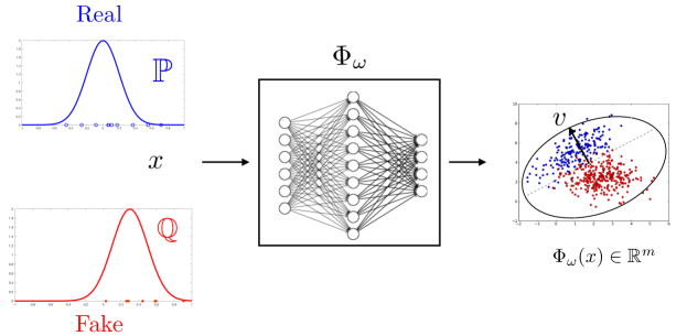
Figure 1: Illustration of Fisher IPM with Neural Networks. ΦωsubscriptΦ𝜔\Phi_{\omega} is a convolutional neural network which defines the embedding space. v𝑣v is the direction in this embedding space with maximal mean separation v,μω()μω()𝑣subscript𝜇𝜔subscript𝜇𝜔\left\langle{v},{\mu_{\omega}(\mathbb{P})-\mu_{\omega}(\mathbb{Q})}\right\rangle, constrained by the hyperellipsoid vΣω(;)v=1superscript𝑣topsubscriptΣ𝜔𝑣1v^{\top}\,\Sigma_{\omega}(\mathbb{P};\mathbb{Q})\,v=1.

2.2 Fisher IPM with Neural Networks

We will specifically study the case where \mathscr{F} is a finite dimensional Hilbert space induced by a neural network ΦωsubscriptΦ𝜔\Phi_{\omega} (see Figure 1 for an illustration). In this case, an IPM with data-independent constraint will be equivalent to mean matching [8]. We will now show that Fisher IPM will give rise to a whitened mean matching interpretation, or equivalently to mean matching with a Mahalanobis distance.

Rayleigh Quotient. Consider the function space v,ωsubscript𝑣𝜔\mathscr{F}_{v,\omega}, defined as follows

v,ω={f(x)=v,Φω(x)|vm,Φω:Xm},subscript𝑣𝜔conditional-set𝑓𝑥𝑣subscriptΦ𝜔𝑥:𝑣superscript𝑚subscriptΦ𝜔Xsuperscriptm\mathscr{F}_{v,\omega}=\{f(x)=\left\langle{v},{\Phi_{\omega}(x)}\right\rangle|v\in\mathbb{R}^{m},\Phi_{\omega}:\pazocal{X}\to\mathbb{R}^{m}\},

ΦωsubscriptΦ𝜔\Phi_{\omega} is typically parametrized with a multi-layer neural network. We define the mean and covariance (Gramian) feature embedding of a distribution as in McGan [8]:

μω()=𝔼x(Φω(x))andΣω()=𝔼x(Φω(x)Φω(x)),formulae-sequencesubscript𝜇𝜔similar-to𝑥𝔼subscriptΦ𝜔𝑥andsubscriptΣ𝜔similar-to𝑥𝔼subscriptΦ𝜔𝑥subscriptΦ𝜔superscript𝑥top\mu_{\omega}(\mathbb{P})=\underset{x\sim\mathbb{P}}{\mathbb{E}}\left(\Phi_{\omega}(x)\right)~{}~{}~{}~{}~{}\text{and}~{}~{}~{}~{}~{}\Sigma_{\omega}(\mathbb{P})=\underset{x\sim\mathbb{P}}{\mathbb{E}}\left(\Phi_{\omega}(x)\Phi_{\omega}(x)^{\top}\right),

Fisher IPM as defined in Equation (2) on v,ωsubscript𝑣𝜔\mathscr{F}_{v,\omega} can be written as follows:

dv,ω(,)=maxωmaxvv,μω()μω()v(12Σω()+12Σω()+γIm)v,subscript𝑑subscript𝑣𝜔subscript𝜔subscript𝑣𝑣subscript𝜇𝜔subscript𝜇𝜔superscript𝑣top12subscriptΣ𝜔12subscriptΣ𝜔𝛾subscript𝐼𝑚𝑣d_{\mathscr{F}_{v,\omega}}(\mathbb{P},\mathbb{Q})=\max_{\omega}\max_{v}\frac{\left\langle{v},{\mu_{\omega}(\mathbb{P})-\mu_{\omega}(\mathbb{Q})}\right\rangle}{\sqrt{v^{\top}(\frac{1}{2}\Sigma_{\omega}(\mathbb{P})+\frac{1}{2}\Sigma_{\omega}(\mathbb{Q})+\gamma I_{m})v}}, (5)

where we added a regularization term (γ>0𝛾0\gamma>0) to avoid singularity of the covariances. Note that if ΦωsubscriptΦ𝜔\Phi_{\omega} was implemented with homogeneous non linearities such as RELU, if we swap (v,ω)𝑣𝜔(v,\omega) with (cv,cω)𝑐𝑣superscript𝑐𝜔(cv,c^{\prime}\omega) for any constants c,c>0𝑐superscript𝑐0c,c^{\prime}>0, the distance dv,ωsubscript𝑑subscript𝑣𝜔d_{\mathscr{F}_{v,\omega}} remains unchanged, hence the scaling invariance.

Constrained Form. Since the Rayleigh Quotient is not amenable to optimization, we will consider Fisher IPM as a constrained optimization problem. By virtue of the scaling invariance and the constrained form of the Fisher IPM given in Equation (3), dv,ωsubscript𝑑subscript𝑣𝜔d_{\mathscr{F}_{v,\omega}} can be written equivalently as:

dv,ω(,)=maxω,v,v(12Σω()+12Σω()+γIm)v=1v,μω()μω()subscript𝑑subscript𝑣𝜔subscript𝜔𝑣superscript𝑣top12subscriptΣ𝜔12subscriptΣ𝜔𝛾subscript𝐼𝑚𝑣1𝑣subscript𝜇𝜔subscript𝜇𝜔d_{\mathscr{F}_{v,\omega}}(\mathbb{P},\mathbb{Q})=\max_{\omega,v,v^{\top}(\frac{1}{2}\Sigma_{\omega}(\mathbb{P})+\frac{1}{2}\Sigma_{\omega}(\mathbb{Q})+\gamma I_{m})v=1}\left\langle{v},{\mu_{\omega}(\mathbb{P})-\mu_{\omega}(\mathbb{Q})}\right\rangle (6)

Define the pooled covariance: Σω(;)=12Σω()+12Σω()+γImsubscriptΣ𝜔12subscriptΣ𝜔12subscriptΣ𝜔𝛾subscript𝐼𝑚\Sigma_{\omega}(\mathbb{P};\mathbb{Q})=\frac{1}{2}\Sigma_{\omega}(\mathbb{P})+\frac{1}{2}\Sigma_{\omega}(\mathbb{Q})+\gamma I_{m}. Doing a simple change of variable u=(Σω(;))12v𝑢superscriptsubscriptΣ𝜔12𝑣u=(\Sigma_{\omega}(\mathbb{P};\mathbb{Q}))^{\frac{1}{2}}v we see that:

du,ω(,)subscript𝑑subscript𝑢𝜔\displaystyle d_{\mathscr{F}_{u,\omega}}(\mathbb{P},\mathbb{Q}) =\displaystyle= maxωmaxu,u=1u,(Σω(;))12(μω()μω())subscript𝜔subscript𝑢delimited-∥∥𝑢1𝑢superscriptsubscriptΣ𝜔12subscript𝜇𝜔subscript𝜇𝜔\displaystyle\max_{\omega}\max_{u,\left\lVert{u}\right\rVert=1}\left\langle{u},{(\Sigma_{\omega}(\mathbb{P};\mathbb{Q}))^{-\frac{1}{2}}\left(\mu_{\omega}(\mathbb{P})-\mu_{\omega}(\mathbb{Q})\right)}\right\rangle (7)
=\displaystyle= maxω(Σω(;))12(μω()μω()),subscript𝜔superscriptsubscriptΣ𝜔12subscript𝜇𝜔subscript𝜇𝜔\displaystyle\max_{\omega}\left\lVert{(\Sigma_{\omega}(\mathbb{P};\mathbb{Q}))^{-\frac{1}{2}}\left(\mu_{\omega}(\mathbb{P})-\mu_{\omega}(\mathbb{Q})\right)}\right\rVert,

hence we see that fisher IPM corresponds to the worst case distance between whitened means. Since the means are white, we don’t need to impose further constraints on ω𝜔\omega as in [6, 8]. Another interpretation of the Fisher IPM stems from the fact that:

dv,ω(,)=maxω(μω()μω())Σω1(;)(μω()μω()),subscript𝑑subscript𝑣𝜔subscript𝜔superscriptsubscript𝜇𝜔subscript𝜇𝜔topsuperscriptsubscriptΣ𝜔1subscript𝜇𝜔subscript𝜇𝜔d_{\mathscr{F}_{v,\omega}}(\mathbb{P},\mathbb{Q})=\max_{\omega}\sqrt{(\mu_{\omega}(\mathbb{P})-\mu_{\omega}(\mathbb{Q}))^{\top}\Sigma_{\omega}^{-1}(\mathbb{P};\mathbb{Q})(\mu_{\omega}(\mathbb{P})-\mu_{\omega}(\mathbb{Q}))},

from which we see that Fisher IPM is a Mahalanobis distance between the mean feature embeddings of the distributions. The Mahalanobis distance is defined by the positive definite matrix Σw(;)subscriptΣ𝑤\Sigma_{w}(\mathbb{P};\mathbb{Q}). We show in Appendix A that the gradient penalty in Improved Wasserstein [7] gives rise to a similar Mahalanobis mean matching interpretation.

Learning GAN with Fisher IPM. Hence we see that learning GAN with Fisher IPM:

mingθmaxωmaxv,v(12Σω(r)+12Σω(θ)+γIm)v=1v,μw(r)μω(θ)subscriptsubscript𝑔𝜃subscript𝜔subscript𝑣superscript𝑣top12subscriptΣ𝜔subscript𝑟12subscriptΣ𝜔subscript𝜃𝛾subscript𝐼𝑚𝑣1𝑣subscript𝜇𝑤subscript𝑟subscript𝜇𝜔subscript𝜃\min_{g_{\theta}}\max_{\omega}\max_{v,v^{\top}(\frac{1}{2}\Sigma_{\omega}(\mathbb{P}_{r})+\frac{1}{2}\Sigma_{\omega}(\mathbb{\mathbb{P}_{\theta}})+\gamma I_{m})v=1}\left\langle{v},{\mu_{w}(\mathbb{P}_{r})-\mu_{\omega}(\mathbb{P}_{\theta})}\right\rangle

corresponds to a min-max game between a feature space and a generator. The feature space tries to maximize the Mahalanobis distance between the feature means embeddings of real and fake distributions. The generator tries to minimize the mean embedding distance.

Refer to caption
Figure 2: Example on 2D synthetic data, where both {\color[rgb]{0,0,1}\definecolor[named]{pgfstrokecolor}{rgb}{0,0,1}\mathbb{P}} and {\color[rgb]{1,0,0}\definecolor[named]{pgfstrokecolor}{rgb}{1,0,0}\mathbb{Q}} are fixed normal distributions with the same covariance and shifted means along the x-axis, see (a). Fig (b, c) show the exact χ2subscript𝜒2\chi_{2} distance from numerically integrating Eq (8), together with the estimate obtained from training a 5-layer MLP with layer size = 16 and LeakyReLU nonlinearity on different training sample sizes. The MLP is trained using Algorithm 1, where sampling from the generator is replaced by sampling from \mathbb{Q}, and the χ2subscript𝜒2\chi_{2} MLP estimate is computed with Equation (2) on a large number of samples (i.e. out of sample estimate). We see in (b) that for large enough sample size, the MLP estimate is extremely good. In (c) we see that for smaller sample sizes, the MLP approximation bounds the ground truth χ2subscript𝜒2\chi_{2} from below (see Theorem 2) and converges to the ground truth roughly as 𝒪(1N)𝒪1𝑁\mathscr{O}(\frac{1}{\sqrt{N}}) (Theorem 3). We notice that when the distributions have small χ2subscript𝜒2\chi_{2} distance, a larger training size is needed to get a better estimate - again this is in line with Theorem 3.

3 Theory

We will start first by studying the Fisher IPM defined in Equation (2) when the function space has full capacity i.e when the critic belongs to 2(X,12(+))subscript2X12\mathscr{L}_{2}(\pazocal{X},\frac{1}{2}(\mathbb{P}+\mathbb{Q})) meaning that Xf2(x)((x)+(x))2𝑑x<subscriptXsuperscript𝑓2𝑥𝑥𝑥2differential-d𝑥\int_{\pazocal{X}}f^{2}(x)\frac{(\mathbb{P}(x)+\mathbb{Q}(x))}{2}dx<\infty. Theorem 1 shows that under this condition, the Fisher IPM corresponds to the Chi-squared distance between distributions, and gives a closed form expression of the optimal critic function fχsubscript𝑓𝜒f_{\chi} (See Appendix B for its relation with the Pearson Divergence). Proofs are given in Appendix D.

Theorem 1 (Chi-squared distance at full capacity).

Consider the Fisher IPM for \mathscr{F} being the space of all measurable functions endowed by 12(+)12\frac{1}{2}(\mathbb{P}+\mathbb{Q}), i.e. :=2(X,+2)assignsubscript2X2\mathscr{F}:=\mathscr{L}_{2}(\pazocal{X},\frac{\mathbb{P}+\mathbb{Q}}{2}). Define the Chi-squared distance between two distributions:

χ2(,)=X((x)(x))2(x)+(x)2𝑑xsubscript𝜒2subscriptXsuperscript𝑥𝑥2𝑥𝑥2differential-d𝑥\chi_{2}(\mathbb{P},\mathbb{Q})=\sqrt{\int_{\pazocal{X}}\frac{(\mathbb{P}(x)-\mathbb{Q}(x))^{2}}{\frac{\mathbb{P}(x)+\mathbb{Q}(x)}{2}}dx} (8)

The following holds true for any ,\mathbb{P},\mathbb{Q}, \mathbb{P}\neq\mathbb{Q}:

1) The Fisher IPM for =2(X,+2)subscript2X2\mathscr{F}=\mathscr{L}_{2}(\pazocal{X},\frac{\mathbb{P}+\mathbb{Q}}{2}) is equal to the Chi-squared distance defined above: d(,)=χ2(,).subscript𝑑subscript𝜒2d_{\mathscr{F}}(\mathbb{P},\mathbb{Q})=\chi_{2}(\mathbb{P},\mathbb{Q}).
2) The optimal critic of the Fisher IPM on 2(X,+2)subscript2X2\mathscr{L}_{2}(\pazocal{X},\frac{\mathbb{P}+\mathbb{Q}}{2}) is :

fχ(x)=1χ2(,)(x)(x)(x)+(x)2.subscript𝑓𝜒𝑥1subscript𝜒2𝑥𝑥𝑥𝑥2f_{\chi}(x)=\frac{1}{\chi_{2}(\mathbb{P},\mathbb{Q})}\frac{\mathbb{P}(x)-\mathbb{Q}(x)}{\frac{\mathbb{P}(x)+\mathbb{Q}(x)}{2}}.

We note here that LSGAN [5] at full capacity corresponds to a Chi-Squared divergence, with the main difference that LSGAN has different objectives for the generator and the discriminator (bilevel optimizaton), and hence does not optimize a single objective that is a distance between distributions. The Chi-squared divergence can also be achieved in the f𝑓f-gan framework from [3]. We discuss the advantages of the Fisher formulation in Appendix C.

Optimizing over 2(X,+2)subscript2X2\mathscr{L}_{2}(\pazocal{X},\frac{\mathbb{P}+\mathbb{Q}}{2}) is not tractable, hence we have to restrict our function class, to a hypothesis class \mathscr{H}, that enables tractable computations. Here are some typical choices of the space ::absent\mathscr{H}: Linear functions in the input features, RKHS, a non linear multilayer neural network with a linear last layer (v,ωsubscript𝑣𝜔\mathscr{F}_{v,\omega}). In this Section we don’t make any assumptions about the function space and show in Theorem 2 how the Chi-squared distance is approximated in \mathscr{H}, and how this depends on the approximation error of the optimal critic fχsubscript𝑓𝜒f_{\chi} in \mathscr{H}.

Theorem 2 (Approximating Chi-squared distance in an arbitrary function space \mathscr{H}).

Let \mathscr{H} be an arbitrary symmetric function space. We define the inner product f,fχ2(X,+2)=Xf(x)fχ(x)(x)+(x)2𝑑xsubscript𝑓subscript𝑓𝜒subscript2X2subscriptX𝑓𝑥subscript𝑓𝜒𝑥𝑥𝑥2differential-d𝑥\left\langle{f},{f_{\chi}}\right\rangle_{\mathscr{L}_{2}(\pazocal{X},\frac{\mathbb{P}+\mathbb{Q}}{2})}=\int_{\pazocal{X}}f(x)f_{\chi}(x)\frac{\mathbb{P}(x)+\mathbb{Q}(x)}{2}dx, which induces the Lebesgue norm. Let 𝕊2(X,+2)subscript𝕊subscript2X2\mathbb{S}_{\mathscr{L}_{2}(\pazocal{X},\frac{\mathbb{P}+\mathbb{Q}}{2})} be the unit sphere in 2(X,+2)subscript2X2\mathscr{L}_{2}(\pazocal{X},\frac{\mathbb{P}+\mathbb{Q}}{2}): 𝕊2(X,+2)={f:X,f2(X,+2)=1}.subscript𝕊subscript2X2conditional-set𝑓formulae-sequenceXsubscriptdelimited-∥∥fsubscript2X21\mathbb{S}_{\mathscr{L}_{2}(\pazocal{X},\frac{\mathbb{P}+\mathbb{Q}}{2})}=\{f:\pazocal{X}\to\mathbb{R},\left\lVert{f}\right\rVert_{\mathscr{L}_{2}(\pazocal{X},\frac{\mathbb{P}+\mathbb{Q}}{2})}=1\}. The fisher IPM defined on an arbitrary function space \mathscr{H} d(,)subscript𝑑d_{\mathscr{H}}(\mathbb{P},\mathbb{Q}), approximates the Chi-squared distance. The approximation quality depends on the cosine of the approximation of the optimal critic fχsubscript𝑓𝜒f_{\chi} in \mathscr{H}. Since \mathscr{H} is symmetric this cosine is always positive (otherwise the same equality holds with an absolute value)

d(,)=χ2(,)supf𝕊2(X,+2)f,fχ2(X,+2),subscript𝑑subscript𝜒2subscriptsupremum𝑓subscript𝕊subscript2X2subscript𝑓subscript𝑓𝜒subscript2X2d_{\mathscr{H}}(\mathbb{P},\mathbb{Q})=\chi_{2}(\mathbb{P},\mathbb{Q})\sup_{f\in\mathscr{H}\cap~{}\mathbb{S}_{\mathscr{L}_{2}(\pazocal{X},\frac{\mathbb{P}+\mathbb{Q}}{2})}}\left\langle{f},{f_{\chi}}\right\rangle_{\mathscr{L}_{2}(\pazocal{X},\frac{\mathbb{P}+\mathbb{Q}}{2})},

Equivalently we have following relative approximation error:

χ2(,)d(,)χ2(,)=12inff𝕊2(X,+2)ffχ2(X,+2)2.subscript𝜒2subscript𝑑subscript𝜒212subscriptinfimum𝑓subscript𝕊subscript2X2subscriptsuperscriptdelimited-∥∥𝑓subscript𝑓𝜒2subscript2X2\frac{\chi_{2}(\mathbb{P},\mathbb{Q})-d_{\mathscr{H}}(\mathbb{P},\mathbb{Q})}{\chi_{2}(\mathbb{P},\mathbb{Q})}=\frac{1}{2}\inf_{f\in\mathscr{H}\cap~{}\mathbb{S}_{\mathscr{L}_{2}(\pazocal{X},\frac{\mathbb{P}+\mathbb{Q}}{2})}}\left\lVert{f-f_{\chi}}\right\rVert^{2}_{\mathscr{L}_{2}(\pazocal{X},\frac{\mathbb{P}+\mathbb{Q}}{2})}.

From Theorem 2, we know that we have always d(,)χ2(,)subscript𝑑subscript𝜒2d_{\mathscr{H}}(\mathbb{P},\mathbb{Q})\leq\chi_{2}(\mathbb{P},\mathbb{Q}). Moreover if the space \mathscr{H} was rich enough to provide a good approximation of the optimal critic fχsubscript𝑓𝜒f_{\chi}, then dsubscript𝑑d_{\mathscr{H}} is a good approximation of the Chi-squared distance χ2subscript𝜒2\chi_{2}.

Generalization bounds for the sample quality of the estimated Fisher IPM from samples from \mathbb{P} and \mathbb{Q} can be done akin to [11], with the main difficulty that for Fisher IPM we have to bound the excess risk of a cost function with data dependent constraints on the function class. We give generalization bounds for learning the Fisher IPM in the supplementary material (Theorem 3, Appendix E). In a nutshell the generalization error of the critic learned in a hypothesis class \mathscr{H} from samples of \mathbb{P} and \mathbb{Q}, decomposes to the approximation error from Theorem 2 and a statistical error that is bounded using data dependent local Rademacher complexities [17] and scales like O(1/n),n=MN/M+N𝑂1𝑛𝑛𝑀𝑁𝑀𝑁O(\sqrt{\nicefrac{{1}}{{n}}}),n=\nicefrac{{MN}}{{M+N}}. We illustrate in Figure 2 our main theoretical claims on a toy problem.

4 Fisher GAN Algorithm using ALM

For any choice of the parametric function class psubscript𝑝\mathscr{F}_{p} (for example v,ωsubscript𝑣𝜔\mathscr{F}_{v,\omega}), note the constraint in Equation (4) by Ω^(fp,gθ)=12Ni=1Nfp2(xi)+12Nj=1Nfp2(gθ(zj)).^Ωsubscript𝑓𝑝subscript𝑔𝜃12𝑁superscriptsubscript𝑖1𝑁subscriptsuperscript𝑓2𝑝subscript𝑥𝑖12𝑁superscriptsubscript𝑗1𝑁subscriptsuperscript𝑓2𝑝subscript𝑔𝜃subscript𝑧𝑗\hat{\Omega}(f_{p},g_{\theta})=\frac{1}{2N}\sum_{i=1}^{N}f^{2}_{p}(x_{i})+\frac{1}{2N}\sum_{j=1}^{N}f^{2}_{p}(g_{\theta}(z_{j})). Define the Augmented Lagrangian [18] corresponding to Fisher GAN objective and constraint given in Equation (4):

LF(p,θ,λ)=^(fp,gθ)+λ(1Ω^(fp,gθ))ρ2(Ω^(fp,gθ)1)2subscriptLFp𝜃𝜆^subscriptfpsubscriptg𝜃𝜆1^Ωsubscriptfpsubscriptg𝜃𝜌2superscript^Ωsubscriptfpsubscriptg𝜃12\pazocal{L}_{F}(p,\theta,\lambda)=\hat{\mathscr{E}}(f_{p},g_{\theta})+\lambda(1-\hat{\Omega}(f_{p},g_{\theta}))-\frac{\rho}{2}(\hat{\Omega}(f_{p},g_{\theta})-1)^{2} (9)

where λ𝜆\lambda is the Lagrange multiplier and ρ>0𝜌0\rho>0 is the quadratic penalty weight. We alternate between optimizing the critic and the generator. Similarly to [7] we impose the constraint when training the critic only. Given θ𝜃\theta, for training the critic we solve maxpminλLF(p,θ,λ).subscript𝑝subscript𝜆subscriptLFp𝜃𝜆\max_{p}\min_{\lambda}\pazocal{L}_{F}(p,\theta,\lambda). Then given the critic parameters p𝑝p we optimize the generator weights θ𝜃\theta to minimize the objective minθ^(fp,gθ).subscript𝜃^subscript𝑓𝑝subscript𝑔𝜃\min_{\theta}\hat{\mathscr{E}}(f_{p},g_{\theta}). We give in Algorithm 1, an algorithm for Fisher GAN, note that we use ADAM [19] for optimizing the parameters of the critic and the generator. We use SGD for the Lagrange multiplier with learning rate ρ𝜌\rho following practices in Augmented Lagrangian [18].

Algorithm 1 Fisher GAN
  Input: ρ𝜌\rho penalty weight, η𝜂\eta Learning rate, ncsubscript𝑛𝑐n_{c} number of iterations for training the critic, N batch size
  Initialize p,θ,λ=0𝑝𝜃𝜆0p,\theta,\lambda=0
  repeat
     for j=1𝑗1j=1 to ncsubscript𝑛𝑐n_{c} do
        Sample a minibatch xi,i=1N,xirformulae-sequencesubscript𝑥𝑖𝑖1𝑁similar-tosubscript𝑥𝑖subscript𝑟x_{i},i=1\dots N,x_{i}\sim\mathbb{P}_{r}
        Sample a minibatch zi,i=1N,zipzformulae-sequencesubscript𝑧𝑖𝑖1𝑁similar-tosubscript𝑧𝑖subscript𝑝𝑧z_{i},i=1\dots N,z_{i}\sim p_{z}
        (gp,gλ)(pLF,λLF)(p,θ,λ)subscript𝑔𝑝subscript𝑔𝜆subscript𝑝subscriptLFsubscript𝜆subscriptLFp𝜃𝜆(g_{p},g_{\lambda})\leftarrow(\nabla_{p}{\pazocal{L}_{F}},\nabla_{\lambda}\pazocal{L}_{F})(p,\theta,\lambda)
        pp+η ADAM (p,gp)𝑝𝑝𝜂 ADAM 𝑝subscript𝑔𝑝p\leftarrow p+\eta\text{ ADAM }(p,g_{p})
        λλρgλ𝜆𝜆𝜌subscript𝑔𝜆\lambda\leftarrow\lambda-\rho g_{\lambda} {SGD rule on λ𝜆\lambda with learning rate ρ𝜌\rho}
     end for
     Sample zi,i=1N,zipzformulae-sequencesubscript𝑧𝑖𝑖1𝑁similar-tosubscript𝑧𝑖subscript𝑝𝑧{z_{i},i=1\dots N,z_{i}\sim p_{z}}
     dθθ^(fp,gθ)=θ1Ni=1Nfp(gθ(zi))subscript𝑑𝜃subscript𝜃^subscript𝑓𝑝subscript𝑔𝜃subscript𝜃1𝑁superscriptsubscript𝑖1𝑁subscript𝑓𝑝subscript𝑔𝜃subscript𝑧𝑖d_{\theta}\leftarrow\nabla_{\theta}\hat{\mathscr{E}}(f_{p},g_{\theta})=-\nabla_{\theta}\frac{1}{N}\sum_{i=1}^{N}f_{p}(g_{\theta}(z_{i}))
     θθη ADAM (θ,dθ)𝜃𝜃𝜂 ADAM 𝜃subscript𝑑𝜃\theta\leftarrow\theta-\eta\text{ ADAM }(\theta,d_{\theta})
  until θ𝜃\theta converges

5 Experiments

We experimentally validate the proposed Fisher GAN. We claim three main results: (1) stable training with a meaningful and stable loss going down as training progresses and correlating with sample quality, similar to [6, 7]. (2) very fast convergence to good sample quality as measured by inception score. (3) competitive semi-supervised learning performance, on par with literature baselines, without requiring normalization of the critic.

We report results on three benchmark datasets: CIFAR-10 [20], LSUN [21] and CelebA [22]. We parametrize the generator gθsubscript𝑔𝜃g_{\theta} and critic f𝑓f with convolutional neural networks following the model design from DCGAN [23]. For 64×64646464\times 64 images (LSUN, CelebA) we use the model architecture in Appendix F.2, for CIFAR-10 we train at a 32×32323232\times 32 resolution using architecture in F.3 for experiments regarding sample quality (inception score), while for semi-supervised learning we use a better regularized discriminator similar to the Openai [9] and ALI [24] architectures, as given in F.4.We used Adam [19] as optimizer for all our experiments, hyper-parameters given in Appendix F.

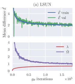
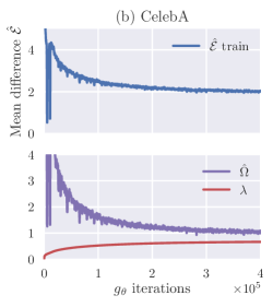
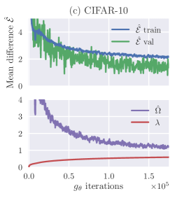
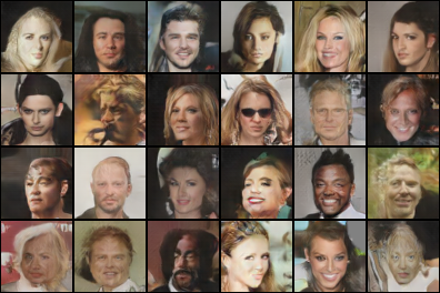
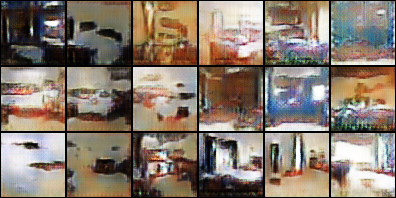
Qualitative: Loss stability and sample quality. Figure 3 shows samples and plots during training. For LSUN we use a higher number of D updates (nc=5subscript𝑛𝑐5n_{c}=5) , since we see similarly to WGAN that the loss shows large fluctuations with lower ncsubscript𝑛𝑐n_{c} values. For CIFAR-10 and CelebA we use reduced nc=2subscript𝑛𝑐2n_{c}=2 with no negative impact on loss stability. CIFAR-10 here was trained without any label information. We show both train and validation loss on LSUN and CIFAR-10 showing, as can be expected, no overfitting on the large LSUN dataset and some overfitting on the small CIFAR-10 dataset. To back up our claim that Fisher GAN provides stable training, we trained both a Fisher Gan and WGAN where the batch normalization in the critic f𝑓f was removed (Figure 4).

Refer to caption
Refer to caption
Refer to caption
Refer to caption
Refer to caption
Refer to caption
Figure 3: Samples and plots of the loss ^(.)\hat{\mathscr{E}}(.), lagrange multiplier λ𝜆\lambda, and constraint Ω^(.)\hat{\Omega}(.) on 3 benchmark datasets. We see that during training as λ𝜆\lambda grows slowly, the constraint becomes tight.
Refer to caption
Refer to caption
Figure 4: No Batch Norm: Training results from a critic f𝑓f without batch normalization. Fisher GAN (left) produces decent samples, while WGAN with weight clipping (right) does not. We hypothesize that this is due to the implicit whitening that Fisher GAN provides. (Note that WGAN-GP does also succesfully converge without BN [7]). For both models the learning rate was appropriately reduced.

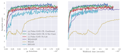
Quantitative analysis: Inception Score and Speed. It is agreed upon that evaluating generative models is hard [25]. We follow the literature in using “inception score” [9] as a metric for the quality of CIFAR-10 samples. Figure 5 shows the inception score as a function of number of gθsubscript𝑔𝜃g_{\theta} updates and wallclock time. All timings are obtained by running on a single K40 GPU on the same cluster. We see from Figure 5, that Fisher GAN both produces better inception scores, and has a clear speed advantage over WGAN-GP.

Quantitative analysis: SSL. One of the main premises of unsupervised learning, is to learn features on a large corpus of unlabeled data in an unsupervised fashion, which are then transferable to other tasks. This provides a proper framework to measure the performance of our algorithm. This leads us to quantify the performance of Fisher GAN by semi-supervised learning (SSL) experiments on CIFAR-10. We do joint supervised and unsupervised training on CIFAR-10, by adding a cross-entropy term to the IPM objective, in conditional and unconditional generation.
Refer to caption
Refer to caption
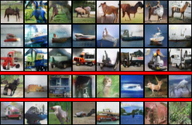
Figure 5: CIFAR-10 inception scores under 3 training conditions. Corresponding samples are given in rows from top to bottom (a,b,c). The inception score plots are mirroring Figure 3 from [7].
Note In v1 of this paper, the baseline inception scores were underestimated because they were computed using too few samples.
Note All inception scores are computed from the same tensorflow codebase, using the architecture described in appendix F.3, and with weight initialization from a normal distribution with stdev=0.02. In Appendix F.1 we show that these choices are also benefiting our WGAN-GP baseline.
Table 2: CIFAR-10 inception scores using resnet architecture and codebase from [7]. We used Layer Normalization [26] which outperformed unnormalized resnets. Apart from this, no additional hyperparameter tuning was done to get stable training of the resnets.
Method Score
ALI [24] 5.34±.05plus-or-minus5.34.055.34\pm.05
BEGAN [27] 5.625.625.62
DCGAN [23] (in [28]) 6.16±.07plus-or-minus6.16.076.16\pm.07
Improved GAN (-L+HA) [9] 6.86±.06plus-or-minus6.86.066.86\pm.06
EGAN-Ent-VI [29] 7.07±.10plus-or-minus7.07.107.07\pm.10
DFM [30] 7.72±.13plus-or-minus7.72.137.72\pm.13
WGAN-GP ResNet [7] 7.86±.07plus-or-minus7.86.077.86\pm.07
Fisher GAN ResNet (ours) 7.90±.05plus-or-minus7.90.057.90\pm.05
    Unsupervised
Method Score
SteinGan [31] 6.356.356.35
DCGAN (with labels, in [31]) 6.586.586.58
Improved GAN [9] 8.09±.07plus-or-minus8.09.078.09\pm.07
Fisher GAN ResNet (ours) 8.16±.12plus-or-minus8.16.128.16\pm.12
AC-GAN [32] 8.25±.07plus-or-minus8.25.078.25\pm.07
SGAN-no-joint [28] 8.37±.08plus-or-minus8.37.088.37\pm.08
WGAN-GP ResNet [7] 8.42±.10plus-or-minus8.42.108.42\pm.10
SGAN [28] 8.59±.12plus-or-minus8.59.128.59\pm.12
    Supervised

Unconditional Generation with CE Regularization. We parametrize the critic f𝑓f as in v,ωsubscript𝑣𝜔\mathscr{F}_{v,\omega}. While training the critic using the Fisher GAN objective LFsubscriptLF\pazocal{L}_{F} given in Equation (9), we train a linear classifier on the feature space ΦωsubscriptΦ𝜔\Phi_{\omega} of the critic, whenever labels are available (K𝐾K labels). The linear classifier is trained with Cross-Entropy (CE) minimization. Then the critic loss becomes LD=LFλD(x,y)labCE(x,y;S,Φω)subscriptLDsubscriptLFsubscript𝜆DsubscriptxylabCExySsubscriptΦ𝜔\pazocal{L}_{D}=\pazocal{L}_{F}-\lambda_{D}\sum_{(x,y)\in\text{lab}}CE(x,y;S,\Phi_{\omega}), where CE(x,y;S,Φω)=log[Softmax(S,Φω(x))y]𝐶𝐸𝑥𝑦𝑆subscriptΦ𝜔SoftmaxsubscriptSsubscriptΦ𝜔xyCE(x,y;S,\Phi_{\omega})=-\log\left[\rm{Softmax}(\left\langle{S},{\Phi_{\omega}(x)}\right\rangle)_{y}\right], where SK×m𝑆superscript𝐾𝑚S\in\mathbb{R}^{K\times m} is the linear classifier and S,ΦωK𝑆subscriptΦ𝜔superscript𝐾\left\langle{S},{\Phi_{\omega}}\right\rangle\in\mathbb{R}^{K} with slight abuse of notation. λDsubscript𝜆𝐷\lambda_{D} is the regularization hyper-parameter. We now sample three minibatches for each critic update: one labeled batch from the small labeled dataset for the CE term, and an unlabeled batch + generated batch for the IPM.

Conditional Generation with CE Regularization. We also trained conditional generator models, conditioning the generator on y𝑦y by concatenating the input noise with a 1-of-K embedding of the label: we now have gθ(z,y)subscript𝑔𝜃𝑧𝑦g_{\theta}(z,y). We parametrize the critic in v,ωsubscript𝑣𝜔\mathscr{F}_{v,\omega} and modify the critic objective as above. We also add a cross-entropy term for the generator to minimize during its training step: LG=^+λGzp(z),yp(y)CE(gθ(z,y),y;S,Φω)subscriptLG^subscript𝜆Gsubscriptformulae-sequencesimilar-tozpzsimilar-toypyCEsubscriptg𝜃zyySsubscriptΦ𝜔\pazocal{L}_{G}=\hat{\mathscr{E}}+\lambda_{G}\sum_{z\sim p(z),y\sim p(y)}CE(g_{\theta}(z,y),y;S,\Phi_{\omega}). For generator updates we still need to sample only a single minibatch since we use the minibatch of samples from gθ(z,y)subscript𝑔𝜃𝑧𝑦g_{\theta}(z,y) to compute both the IPM loss ^^\mathscr{\hat{E}} and CE. The labels are sampled according to the prior yp(y)similar-to𝑦𝑝𝑦y\sim p(y), which defaults to the discrete uniform prior when there is no class imbalance. We found λD=λG=0.1subscript𝜆𝐷subscript𝜆𝐺0.1\lambda_{D}=\lambda_{G}=0.1 to be optimal.

New Parametrization of the Critic: “K+1𝐾1K+1 SSL”. One specific successful formulation of SSL in the standard GAN framework was provided in [9], where the discriminator classifies samples into K+1𝐾1K+1 categories: the K𝐾K correct clases, and K+1𝐾1K+1 for fake samples. Intuitively this puts the real classes in competition with the fake class. In order to implement this idea in the Fisher framework, we define a new function class of the critic that puts in competition the K𝐾K class directions of the classifier Sysubscript𝑆𝑦S_{y}, and another “K+1” direction v𝑣v that indicates fake samples. Hence we propose the following parametrization for the critic: f(x)=y=1Kp(y|x)Sy,Φω(x)v,Φω(x)𝑓𝑥superscriptsubscript𝑦1𝐾𝑝conditional𝑦𝑥subscript𝑆𝑦subscriptΦ𝜔𝑥𝑣subscriptΦ𝜔𝑥f(x)=\sum_{y=1}^{K}p(y|x)\left\langle{S_{y}},{\Phi_{\omega}(x)}\right\rangle-\left\langle{v},{\Phi_{\omega}(x)}\right\rangle, where p(y|x)=Softmax(S,Φω(x))y𝑝conditional𝑦𝑥SoftmaxsubscriptSsubscriptΦ𝜔xyp(y|x)=\rm{Softmax}(\left\langle{S},{\Phi_{\omega}(x)}\right\rangle)_{y} which is also optimized with Cross-Entropy. Note that this critic does not fall under the interpretation with whitened means from Section 2.2, but does fall under the general Fisher IPM framework from Section 2.1. We can use this critic with both conditional and unconditional generation in the same way as described above. In this setting we found λD=1.5,λG=0.1formulae-sequencesubscript𝜆𝐷1.5subscript𝜆𝐺0.1\lambda_{D}=1.5,\,\lambda_{G}=0.1 to be optimal.

Layerwise normalization on the critic. For most GAN formulations following DCGAN design principles, batch normalization (BN) [33] in the critic is an essential ingredient. From our semi-supervised learning experiments however, it appears that batch normalization gives substantially worse performance than layer normalization (LN) [26] or even no layerwise normalization. We attribute this to the implicit whitening Fisher GAN provides.

Table 3 shows the SSL results on CIFAR-10. We show that Fisher GAN has competitive results, on par with state of the art literature baselines. When comparing to WGAN with weight clipping, it becomes clear that we recover the lost SSL performance. Results with the K+1𝐾1K+1 critic are better across the board, proving consistently the advantage of our proposed K+1𝐾1K+1 formulation. Conditional generation does not provide gains in the setting with layer normalization or without normalization.

Table 3: CIFAR-10 SSL results.
Note In v3, strong results were added using LN and no normalization.
Number of labeled examples 1000 2000 4000 8000
Model Misclassification rate
CatGAN [34] 19.5819.5819.58
Improved GAN (FM) [9] 21.83±2.01plus-or-minus21.832.0121.83\pm 2.01 19.61±2.09plus-or-minus19.612.0919.61\pm 2.09 18.63±2.32plus-or-minus18.632.3218.63\pm 2.32 17.72±1.82plus-or-minus17.721.8217.72\pm 1.82
ALI [24] 19.98±0.89plus-or-minus19.980.8919.98\pm 0.89 19.09±0.44plus-or-minus19.090.4419.09\pm 0.44 17.99±1.62plus-or-minus17.991.6217.99\pm 1.62 17.05±1.49plus-or-minus17.051.4917.05\pm 1.49
WGAN (weight clipping) Uncond 69.01 56.48 40.85 30.56
WGAN (weight clipping) Cond 68.11 58.59 42.00 30.91
Fisher GAN BN Cond 36.3736.3736.37 32.0332.0332.03 27.4227.4227.42 22.8522.8522.85
Fisher GAN BN Uncond 36.4236.4236.42 33.4933.4933.49 27.3627.3627.36 22.8222.8222.82
Fisher GAN BN K+1 Cond 34.9434.9434.94 28.0428.0428.04 23.8523.8523.85 20.7520.7520.75
Fisher GAN BN K+1 Uncond 33.4933.4933.49 28.6028.6028.60 24.1924.1924.19 21.5921.5921.59
Fisher GAN LN Cond 26.78±1.04plus-or-minus26.781.0426.78\pm 1.04 23.30±0.39plus-or-minus23.300.3923.30\pm 0.39 20.56±0.64plus-or-minus20.560.6420.56\pm 0.64 18.26±0.25plus-or-minus18.260.2518.26\pm 0.25
Fisher GAN LN Uncond 24.39±1.22plus-or-minus24.391.2224.39\pm 1.22 22.69±1.27plus-or-minus22.691.2722.69\pm 1.27 19.53±0.34plus-or-minus19.530.3419.53\pm 0.34 17.84±0.15plus-or-minus17.840.1517.84\pm 0.15
Fisher GAN LN K+1 Cond 20.99±0.66plus-or-minus20.990.6620.99\pm 0.66 19.01±0.21plus-or-minus19.010.2119.01\pm 0.21 17.41±0.38plus-or-minus17.410.3817.41\pm 0.38 15.50±0.41plus-or-minus15.500.4115.50\pm 0.41
Fisher GAN LN K+1, Uncond 19.74±0.21plus-or-minus19.740.2119.74\pm 0.21 17.87±0.38plus-or-minus17.870.3817.87\pm 0.38 16.13±0.53plus-or-minus16.130.5316.13\pm 0.53 14.81±0.16plus-or-minus14.810.1614.81\pm 0.16
Fisher GAN No Norm K+1, Uncond 21.15±0.54plus-or-minus21.150.5421.15\pm 0.54 18.21±0.30plus-or-minus18.210.3018.21\pm 0.30 16.74±0.19plus-or-minus16.740.1916.74\pm 0.19 14.80±0.15plus-or-minus14.800.1514.80\pm 0.15

6 Conclusion

We have defined Fisher GAN, which provide a stable and fast way of training GANs. The Fisher GAN is based on a scale invariant IPM, by constraining the second order moments of the critic. We provide an interpretation as whitened (Mahalanobis) mean feature matching and χ2subscript𝜒2\chi_{2} distance. We show graceful theoretical and empirical advantages of our proposed Fisher GAN.

Acknowledgments.

The authors thank Steven J. Rennie for many helpful discussions and Martin Arjovsky for helpful clarifications and pointers.

References

  • [1] Ian Goodfellow, Jean Pouget-Abadie, Mehdi Mirza, Bing Xu, David Warde-Farley, Sherjil Ozair, Aaron Courville, and Yoshua Bengio. Generative adversarial nets. In NIPS, 2014.
  • [2] Martin Arjovsky and Léon Bottou. Towards principled methods for training generative adversarial networks. In ICLR, 2017.
  • [3] Sebastian Nowozin, Botond Cseke, and Ryota Tomioka. f-gan: Training generative neural samplers using variational divergence minimization. In NIPS, 2016.
  • [4] Casper Kaae Sønderby, Jose Caballero, Lucas Theis, Wenzhe Shi, and Ferenc Huszár. Amortised map inference for image super-resolution. ICLR, 2017.
  • [5] Xudong Mao, Qing Li, Haoran Xie, Raymond YK Lau, and Zhen Wang. Least squares generative adversarial networks. arXiv:1611.04076, 2016.
  • [6] Martin Arjovsky, Soumith Chintala, and Léon Bottou. Wasserstein gan. ICML, 2017.
  • [7] Ishaan Gulrajani, Faruk Ahmed, Martin Arjovsky, Vincent Dumoulin, and Aaron Courville. Improved training of wasserstein gans. arXiv:1704.00028, 2017.
  • [8] Youssef Mroueh, Tom Sercu, and Vaibhava Goel. Mcgan: Mean and covariance feature matching gan. arXiv:1702.08398 ICML, 2017.
  • [9] Tim Salimans, Ian Goodfellow, Wojciech Zaremba, Vicki Cheung, Alec Radford, and Xi Chen. Improved techniques for training gans. NIPS, 2016.
  • [10] Alfred Müller. Integral probability metrics and their generating classes of functions. Advances in Applied Probability, 1997.
  • [11] Bharath K. Sriperumbudur, Kenji Fukumizu, Arthur Gretton, Bernhard Schölkopf, and Gert R. G. Lanckriet. On the empirical estimation of integral probability metrics. Electronic Journal of Statistics, 2012.
  • [12] Shakir Mohamed and Balaji Lakshminarayanan. Learning in implicit generative models. arXiv:1610.03483, 2016.
  • [13] Arthur Gretton, Karsten M Borgwardt, Malte J Rasch, Bernhard Schölkopf, and Alexander Smola. A kernel two-sample test. JMLR, 2012.
  • [14] Yujia Li, Kevin Swersky, and Richard Zemel. Generative moment matching networks. In ICML, 2015.
  • [15] Gintare Karolina Dziugaite, Daniel M Roy, and Zoubin Ghahramani. Training generative neural networks via maximum mean discrepancy optimization. UAI, 2015.
  • [16] Zaïd Harchaoui, Francis R Bach, and Eric Moulines. Testing for homogeneity with kernel fisher discriminant analysis. In NIPS, 2008.
  • [17] Peter L. Bartlett, Olivier Bousquet, and Shahar Mendelson. Local rademacher complexities. Ann. Statist., 2005.
  • [18] J. Nocedal and S. J. Wright. Numerical Optimization. Springer, 2nd edition, 2006.
  • [19] Diederik Kingma and Jimmy Ba. Adam: A method for stochastic optimization. In ICLR, 2015.
  • [20] A. Krizhevsky and G. Hinton. Learning multiple layers of features from tiny images. Master’s thesis, 2009.
  • [21] Fisher Yu, Ari Seff, Yinda Zhang, Shuran Song, Thomas Funkhouser, and Jianxiong Xiao. Lsun: Construction of a large-scale image dataset using deep learning with humans in the loop. arXiv:1506.03365, 2015.
  • [22] Ziwei Liu, Ping Luo, Xiaogang Wang, and Xiaoou Tang. Deep learning face attributes in the wild. In ICCV, 2015.
  • [23] Alec Radford, Luke Metz, and Soumith Chintala. Unsupervised representation learning with deep convolutional generative adversarial networks. arXiv:1511.06434, 2015.
  • [24] Vincent Dumoulin, Ishmael Belghazi, Ben Poole, Alex Lamb, Martin Arjovsky, Olivier Mastropietro, and Aaron Courville. Adversarially learned inference. ICLR, 2017.
  • [25] Lucas Theis, Aäron van den Oord, and Matthias Bethge. A note on the evaluation of generative models. ICLR, 2016.
  • [26] Jimmy Lei Ba, Jamie Ryan Kiros, and Geoffrey E Hinton. Layer normalization. arXiv preprint arXiv:1607.06450, 2016.
  • [27] David Berthelot, Tom Schumm, and Luke Metz. Began: Boundary equilibrium generative adversarial networks. arXiv preprint arXiv:1703.10717, 2017.
  • [28] Xun Huang, Yixuan Li, Omid Poursaeed, John Hopcroft, and Serge Belongie. Stacked generative adversarial networks. arXiv preprint arXiv:1612.04357, 2016.
  • [29] Zihang Dai, Amjad Almahairi, Philip Bachman, Eduard Hovy, and Aaron Courville. Calibrating energy-based generative adversarial networks. arXiv preprint arXiv:1702.01691, 2017.
  • [30] D Warde-Farley and Y Bengio. Improving generative adversarial networks with denoising feature matching. ICLR submissions, 8, 2017.
  • [31] Dilin Wang and Qiang Liu. Learning to draw samples: With application to amortized mle for generative adversarial learning. arXiv preprint arXiv:1611.01722, 2016.
  • [32] Augustus Odena, Christopher Olah, and Jonathon Shlens. Conditional image synthesis with auxiliary classifier gans. arXiv preprint arXiv:1610.09585, 2016.
  • [33] Sergey Ioffe and Christian Szegedy. Batch normalization: Accelerating deep network training by reducing internal covariate shift. Proc. ICML, 2015.
  • [34] Jost Tobias Springenberg. Unsupervised and semi-supervised learning with categorical generative adversarial networks. arXiv:1511.06390, 2015.
  • [35] Alessandra Tosi, Søren Hauberg, Alfredo Vellido, and Neil D. Lawrence. Metrics for probabilistic geometries. 2014.
  • [36] Bharath K. Sriperumbudur, Kenji Fukumizu, Arthur Gretton, Bernhard Scholkopf, and Gert R. G. Lanckriet. On integral probability metrics, ϕitalic-ϕ\phi-divergences and binary classification. 2009.
  • [37] I. Ekeland and T. Turnbull. Infinite-dimensional Optimization and Convexity. The University of Chicago Press, 1983.
  • [38] Xavier Glorot and Yoshua Bengio. Understanding the difficulty of training deep feedforward neural networks. In International conference on artificial intelligence and statistics, pages 249–256, 2010.
  • [39] Kaiming He, Xiangyu Zhang, Shaoqing Ren, and Jian Sun. Delving deep into rectifiers: Surpassing human-level performance on imagenet classification. arXiv preprint arXiv:1502.01852, 2015.

Supplementary Material for Fisher GAN
Youssef Mroueh, Tom Sercu

IBM Research AI

Appendix A WGAN-GP versus Fisher GAN

Consider

v,ω={f(x)=v,Φw(x),vm,Φω:Xdm}subscript𝑣𝜔conditional-setformulae-sequence𝑓𝑥𝑣subscriptΦ𝑤𝑥𝑣superscript𝑚subscriptΦ𝜔Xsuperscriptdsuperscriptm\mathscr{F}_{v,\omega}=\{f(x)=\left\langle{v},{\Phi_{w}(x)}\right\rangle,v\in\mathbb{R}^{m},\Phi_{\omega}:\pazocal{X}\subset\mathbb{R}^{d}\to\mathbb{R}^{m}\}

Let

JΦω(x)m×d,[JΦω(x)]i,j=ei,Φω(x)xjformulae-sequencesubscript𝐽subscriptΦ𝜔𝑥superscript𝑚𝑑subscriptdelimited-[]subscript𝐽subscriptΦ𝜔𝑥𝑖𝑗subscript𝑒𝑖subscriptΦ𝜔𝑥subscript𝑥𝑗J_{\Phi_{\omega}}(x)\in\mathbb{R}^{m\times d},[J_{\Phi_{\omega}}(x)]_{i,j}=\frac{\partial\left\langle{e_{i}},{\Phi_{\omega}(x)}\right\rangle}{\partial x_{j}}

be the Jacobian matrix of the Φω(.)\Phi_{\omega}(.). It is easy to see that

xf(x)=JΦω(x)vd,subscript𝑥𝑓𝑥subscriptsuperscript𝐽topsubscriptΦ𝜔𝑥𝑣superscript𝑑\nabla_{x}f(x)=J^{\top}_{\Phi_{\omega}}(x)v\in\mathbb{R}^{d},

and therefore

xf(x)2=v,JΦω(x)JΦω(x)v,superscriptdelimited-∥∥subscript𝑥𝑓𝑥2𝑣subscript𝐽subscriptΦ𝜔𝑥subscriptsuperscript𝐽topsubscriptΦ𝜔𝑥𝑣\left\lVert{\nabla_{x}f(x)}\right\rVert^{2}=\left\langle{v},{J_{\Phi_{\omega}}(x)J^{\top}_{\Phi_{\omega}}(x)v}\right\rangle,

Note that ,

JΦω(x)JΦω(x)subscript𝐽subscriptΦ𝜔𝑥subscriptsuperscript𝐽topsubscriptΦ𝜔𝑥J_{\Phi_{\omega}}(x)J^{\top}_{\Phi_{\omega}}(x)

is the so called metric tensor in information geometry (See for instance [35] and references there in). The gradient penalty for WGAN of [7] can be derived from a Rayleigh quotient principle as well, written in the constraint form:

dv,ω(,)=supfv,ω,𝔼uU[0,1]𝔼xu+(1u)xf(x)2=1𝔼xf(x)𝔼xf(x)subscript𝑑subscript𝑣𝜔subscriptsupremumformulae-sequence𝑓subscript𝑣𝜔subscript𝔼similar-to𝑢𝑈01subscript𝔼similar-to𝑥𝑢1𝑢superscriptdelimited-∥∥subscript𝑥𝑓𝑥21subscript𝔼similar-to𝑥𝑓𝑥subscript𝔼similar-to𝑥𝑓𝑥d_{\mathscr{F}_{v,\omega}}(\mathbb{P},\mathbb{Q})=\sup_{f\in\mathscr{F}_{v,\omega},\mathbb{E}_{u\sim U[0,1]}\mathbb{E}_{x\sim u\mathbb{P}+(1-u)\mathbb{Q}}\left\lVert{\nabla_{x}f(x)}\right\rVert^{2}=1}\mathbb{E}_{x\sim\mathbb{P}}f(x)-\mathbb{E}_{x\sim\mathbb{Q}}f(x)

Using the special parametrization we can write:

𝔼uU[0,1]𝔼xu+(1u)xf(x)2=v(𝔼uU[0,1]𝔼xu+(1u)JΦω(x)JΦω(x))vsubscript𝔼similar-to𝑢𝑈01subscript𝔼similar-to𝑥𝑢1𝑢superscriptdelimited-∥∥subscript𝑥𝑓𝑥2superscript𝑣topsubscript𝔼similar-to𝑢𝑈01subscript𝔼similar-to𝑥𝑢1𝑢subscript𝐽subscriptΦ𝜔𝑥subscriptsuperscript𝐽topsubscriptΦ𝜔𝑥𝑣\mathbb{E}_{u\sim U[0,1]}\mathbb{E}_{x\sim u\mathbb{P}+(1-u)\mathbb{Q}}\left\lVert{\nabla_{x}f(x)}\right\rVert^{2}=v^{\top}\left(\mathbb{E}_{u\sim U[0,1]}\mathbb{E}_{x\sim u\mathbb{P}+(1-u)\mathbb{Q}}J_{\Phi_{\omega}}(x)J^{\top}_{\Phi_{\omega}}(x)\right)v

Let

ω(;)=𝔼uU[0,1]𝔼xu+(1u)JΦω(x)JΦω(x)m×msubscript𝜔subscript𝔼similar-to𝑢𝑈01subscript𝔼similar-to𝑥𝑢1𝑢subscript𝐽subscriptΦ𝜔𝑥subscriptsuperscript𝐽topsubscriptΦ𝜔𝑥superscript𝑚𝑚\mathscr{M}_{\omega}(\mathbb{P};\mathbb{Q})=\mathbb{E}_{u\sim U[0,1]}\mathbb{E}_{x\sim u\mathbb{P}+(1-u)\mathbb{Q}}J_{\Phi_{\omega}}(x)J^{\top}_{\Phi_{\omega}}(x)\in\mathbb{R}^{m\times m}

is the expected Riemannian metric tensor [35]. Hence we obtain:

dv,ω(,)subscript𝑑subscript𝑣𝜔\displaystyle d_{\mathscr{F}_{v,\omega}}(\mathbb{P},\mathbb{Q}) =maxwmaxv,vω(;)v=1v,μω()μω()absentsubscript𝑤subscript𝑣superscript𝑣topsubscript𝜔𝑣1𝑣subscript𝜇𝜔subscript𝜇𝜔\displaystyle=\max_{w}\max_{v,v^{\top}\mathscr{M}_{\omega}(\mathbb{P};\mathbb{Q})v=1}\left\langle{v},{\mu_{\omega}(\mathbb{P})-\mu_{\omega}(\mathbb{Q})}\right\rangle
=maxωω12(;)(μω())μω()absentsubscript𝜔subscriptsuperscript12𝜔subscript𝜇𝜔subscript𝜇𝜔\displaystyle=\max_{\omega}\left\lVert{\mathscr{M}^{-\frac{1}{2}}_{\omega}(\mathbb{P};\mathbb{Q})(\mu_{\omega}(\mathbb{P}))-\mu_{\omega}(\mathbb{Q})}\right\rVert

Hence Gradient penalty can be seen as well as mean matching in the metric defined by the expected metric tensor ωsubscript𝜔\mathscr{M}_{\omega}.

Improved WGAN [7] IPM can be written as follows :

maxω(μω()μω())ω1(;)(μω()μω())subscript𝜔superscriptsubscript𝜇𝜔subscript𝜇𝜔topsuperscriptsubscript𝜔1subscript𝜇𝜔subscript𝜇𝜔\max_{\omega}\sqrt{(\mu_{\omega}(\mathbb{P})-\mu_{\omega}(\mathbb{Q}))^{\top}\mathscr{M}_{\omega}^{-1}(\mathbb{P};\mathbb{Q})(\mu_{\omega}(\mathbb{P})-\mu_{\omega}(\mathbb{Q}))}

to be contrasted with Fisher IPM:

maxω(μω()μω())Σω1(;)(μω()μω())subscript𝜔superscriptsubscript𝜇𝜔subscript𝜇𝜔topsuperscriptsubscriptΣ𝜔1subscript𝜇𝜔subscript𝜇𝜔\max_{\omega}\sqrt{(\mu_{\omega}(\mathbb{P})-\mu_{\omega}(\mathbb{Q}))^{\top}\Sigma_{\omega}^{-1}(\mathbb{P};\mathbb{Q})(\mu_{\omega}(\mathbb{P})-\mu_{\omega}(\mathbb{Q}))}

Both Improved WGAN are doing mean matching using different Mahalanobis distances! While improved WGAN uses an expected metric tensor ωsubscript𝜔\mathscr{M}_{\omega} to compute this distance, Fisher IPM uses a simple pooled covariance ΣωsubscriptΣ𝜔\Sigma_{\omega} to compute this metric. It is clear that Fisher GAN has a computational advantage!

Appendix B Chi-squared distance and Pearson Divergence

The definition of χ2subscript𝜒2\chi_{2} distance:

χ22(,)=2X((x)(x))2(x)+(x)𝑑x.superscriptsubscript𝜒222subscriptXsuperscript𝑥𝑥2𝑥𝑥differential-d𝑥\chi_{2}^{2}(\mathbb{P},\mathbb{Q})=2\int_{\pazocal{X}}\frac{(\mathbb{P}(x)-\mathbb{Q}(x))^{2}}{\mathbb{P}(x)+\mathbb{Q}(x)}dx.

The χ2subscript𝜒2\chi_{2} Pearson divergence:

χ2P(,)=X((x)(x))2(x)𝑑x.subscriptsuperscript𝜒𝑃2subscriptXsuperscript𝑥𝑥2𝑥differential-d𝑥\chi^{P}_{2}(\mathbb{P},\mathbb{Q})=\int_{\pazocal{X}}\frac{(\mathbb{P}(x)-\mathbb{Q}(x))^{2}}{\mathbb{Q}(x)}dx.

We have the following relation:

χ22(,)=14χ2P(,+2).subscriptsuperscript𝜒2214subscriptsuperscript𝜒𝑃22\chi^{2}_{2}(\mathbb{P},\mathbb{Q})=\frac{1}{4}\chi^{P}_{2}\left(\mathbb{P},\frac{\mathbb{P}+\mathbb{Q}}{2}\right).

Appendix C Fisher GAN and φ𝜑\varphi-divergence Based GANs

Since f𝑓f-gan [3] also introduces a GAN formulation which recovers the Chi-squared divergence, we compare our approaches.

Let us recall here the definition of φ𝜑\varphi-divergence:

dφ(,)=Xφ((x)(x))(x)𝑑x,subscript𝑑𝜑subscriptX𝜑𝑥𝑥𝑥differential-d𝑥d_{\varphi}(\mathbb{P},\mathbb{Q})=\int_{\pazocal{X}}\varphi\left(\frac{\mathbb{P}(x)}{\mathbb{Q}(x)}\right)\mathbb{Q}(x)dx,

where φ:+:𝜑superscript\varphi:\mathbb{R}^{+}\to\mathbb{R} is a convex, lower-semicontinuous function satisfying φ(1)=0𝜑10\varphi(1)=0. Let φsuperscript𝜑\varphi^{*} the Fenchel conjugate of φ𝜑\varphi:

φ(t)=supuDomφutφ(u)superscript𝜑𝑡subscriptsupremum𝑢𝐷𝑜subscript𝑚𝜑𝑢𝑡𝜑𝑢\varphi^{*}(t)=\sup_{u\in Dom_{\varphi}}{ut-\varphi(u)}

As shown in [3] and in [36], for any function space \mathscr{F} we get the lower bound:

dφ(,)supf𝔼xf(x)𝔼xφ(f(x)),subscript𝑑𝜑subscriptsupremum𝑓subscript𝔼similar-to𝑥𝑓𝑥subscript𝔼similar-to𝑥superscript𝜑𝑓𝑥d_{\varphi}(\mathbb{P},\mathbb{Q})\geq\sup_{f\in\mathscr{F}}\mathbb{E}_{x\sim\mathbb{P}}f(x)-\mathbb{E}_{x\sim\mathbb{Q}}\varphi^{*}(f(x)),

For the particular case φ(t)=(t1)2𝜑𝑡superscript𝑡12\varphi(t)=(t-1)^{2} and φ(t)=14t2+tsuperscript𝜑𝑡14superscript𝑡2𝑡\varphi^{*}(t)=\frac{1}{4}t^{2}+t we have the Pearson χ2subscript𝜒2\chi_{2} divergence:

dφ(,)=X((x)(x))2(x)𝑑x=χ2P(,)subscript𝑑𝜑subscriptXsuperscript𝑥𝑥2𝑥differential-d𝑥subscriptsuperscript𝜒𝑃2d_{\varphi}(\mathbb{P},\mathbb{Q})=\int_{\pazocal{X}}\frac{(\mathbb{P}(x)-\mathbb{Q}(x))^{2}}{\mathbb{Q}(x)}dx=\chi^{P}_{2}(\mathbb{P},\mathbb{Q})

Hence to optimize the same cost function of Fisher GAN in the φ𝜑\varphi-GAN framework we have to consider:

12χ2P(,+2),12subscriptsuperscript𝜒𝑃22\frac{1}{2}\sqrt{\chi^{{P}}_{2}\left(\mathbb{P},\frac{\mathbb{P}+\mathbb{Q}}{2}\right)},

Fisher GAN gives an inequality for the symmetric Chi-squared and the φ𝜑\varphi-GAN gives a lower variational bound. i.e compare for φ𝜑\varphi-GAN:

supf𝔼xf(x)𝔼x+2φ(f(x))subscriptsupremum𝑓subscript𝔼similar-to𝑥𝑓𝑥subscript𝔼similar-to𝑥2superscript𝜑𝑓𝑥\displaystyle\sup_{f\in\mathscr{F}}\mathbb{E}_{x\sim\mathbb{P}}f(x)-\mathbb{E}_{x\sim\frac{\mathbb{P}+\mathbb{Q}}{2}}\varphi^{*}(f(x)) =supf𝔼xf(x)𝔼x+2(14f2(x)+f(x))absentsubscriptsupremum𝑓subscript𝔼similar-to𝑥𝑓𝑥subscript𝔼similar-to𝑥214superscript𝑓2𝑥𝑓𝑥\displaystyle=\sup_{f\in\mathscr{F}}\mathbb{E}_{x\sim\mathbb{P}}f(x)-\mathbb{E}_{x\sim\frac{\mathbb{P}+\mathbb{Q}}{2}}\left(\frac{1}{4}f^{2}(x)+f(x)\right)
=supf12(𝔼xf(x)𝔼xf(x))14𝔼x+2f2(x)absentsubscriptsupremum𝑓12subscript𝔼similar-to𝑥𝑓𝑥subscript𝔼similar-to𝑥𝑓𝑥14subscript𝔼similar-to𝑥2superscript𝑓2𝑥\displaystyle=\sup_{f\in\mathscr{F}}\frac{1}{2}\left(\mathbb{E}_{x\sim\mathbb{P}}f(x)-\mathbb{E}_{x\sim\mathbb{Q}}f(x)\right)-\frac{1}{4}\mathbb{E}_{x\sim\frac{\mathbb{P}+\mathbb{Q}}{2}}f^{2}(x) (10)

and for Fisher GAN:

supf,𝔼x+2f2(x)=1𝔼xf(x)𝔼x(f(x))subscriptsupremumformulae-sequence𝑓subscript𝔼similar-to𝑥2superscript𝑓2𝑥1subscript𝔼similar-to𝑥𝑓𝑥subscript𝔼similar-to𝑥𝑓𝑥\sup_{f\in\mathscr{F},\mathbb{E}_{x\sim\frac{\mathbb{P}+\mathbb{Q}}{2}}f^{2}(x)=1}\mathbb{E}_{x\sim\mathbb{P}}f(x)-\mathbb{E}_{x\sim\mathbb{Q}}(f(x)) (11)

while equivalent at the optimum those two formulations for the symmetric Chi-squared given in Equations (10), and (11) have different theoretical and practical properties. On the theory side:

  1. 1.

    While the formulation in (10) is a φ𝜑\varphi divergence, the formulation given by the Fisher criterium in (11) is an IPM with a data dependent constraint. This is a surprising result because φ𝜑\varphi-divergences and IPM exhibit different properties and the only known non trivial φ𝜑\varphi divergence that is also an IPM with data independent function class is the total variation distance [36]. When we allow the function class to be dependent on the distributions, the symmetric Chi-squared divergence (in fact general Chi-squared also) can be cast as an IPM! Hence in the context of GAN training we inherit the known stability of IPM based training for GANs.

  2. 2.

    Theorem 2 for the Fisher criterium gives us an approximation error when we change the function from the space of measurable functions to a hypothesis class. It is not clear how tight the lower bound in the φ𝜑\varphi-divergence will be as we relax the function class.

On the practical side:

  1. 1.

    Once we parametrize the critic f𝑓f as a neural network with linear output activation, i.e. f(x)=v,Φω(x)𝑓𝑥𝑣subscriptΦ𝜔𝑥f(x)=\left\langle{v},{\Phi_{\omega}(x)}\right\rangle, we see that the optimization is unconstrained for the φ𝜑\varphi-divergence formulation (10) and the weights updates can explode and have an unstable behavior. On the other hand in the Fisher formulation (11) the data dependent constraint that is imposed slowly through the lagrange multiplier, enforces a variance control that prevents the critic from blowing up and causing instabilities in the training. Note that in the Fisher case we have three players: the critic, the generator and the lagrange multiplier. The lagrange multiplier grows slowly to enforce the constraint and to approach the Chi-squared distance as training converges. Note that the φ𝜑\varphi-divergence formulation (10) can be seen as a Fisher GAN with fixed lagrange multiplier λ=12𝜆12\lambda=\frac{1}{2} that is indeed unstable in theory and in our experiments.

Remark 1.

Note that if the Neyman divergence is of interest, it can also be obtained as the following Fisher criterium:

supf,𝔼xf2(x)=1𝔼xf(x)𝔼x(f(x)),subscriptsupremumformulae-sequence𝑓subscript𝔼similar-to𝑥superscript𝑓2𝑥1subscript𝔼similar-to𝑥𝑓𝑥subscript𝔼similar-to𝑥𝑓𝑥\sup_{f\in\mathscr{F},\mathbb{E}_{x\sim\mathbb{P}}f^{2}(x)=1}\mathbb{E}_{x\sim\mathbb{P}}f(x)-\mathbb{E}_{x\sim\mathbb{Q}}(f(x)), (12)

this is equivalent at the optimum to:

χ2N(,)=X((x)(x))2(x)𝑑x.subscriptsuperscript𝜒𝑁2subscriptXsuperscript𝑥𝑥2𝑥differential-d𝑥\chi^{N}_{2}(\mathbb{P},\mathbb{Q})=\int_{\pazocal{X}}\frac{(\mathbb{P}(x)-\mathbb{Q}(x))^{2}}{\mathbb{P}(x)}dx.

Using a neural network f(x)=v,Φω(x)𝑓𝑥𝑣subscriptΦ𝜔𝑥f(x)=\left\langle{v},{\Phi_{\omega}(x)}\right\rangle, the Neyman divergence can be achieved with linear output activation and a data dependent constraint:

supv,ω,𝔼x(v,Φω(x))2=1v,𝔼xΦω(x)𝔼xΦω(x)subscriptsupremum𝑣𝜔subscript𝔼similar-to𝑥superscript𝑣subscriptΦ𝜔𝑥21𝑣subscript𝔼similar-to𝑥subscriptΦ𝜔𝑥subscript𝔼similar-to𝑥subscriptΦ𝜔𝑥\sup_{v,\omega,~{}\mathbb{E}_{x\sim\mathbb{P}}(\left\langle{v},{\Phi_{\omega}(x)}\right\rangle)^{2}=1}\left\langle{v},{\mathbb{E}_{x\sim\mathbb{P}}\Phi_{\omega}(x)-\mathbb{E}_{x\sim\mathbb{Q}}\Phi_{\omega}(x)}\right\rangle

To obtain the same divergence as a φ𝜑\varphi-divergence we need φ(u)=(1u)2u𝜑𝑢superscript1𝑢2𝑢\varphi(u)=\frac{(1-u)^{2}}{u}, and φ(u)=221u,(u<1).superscript𝜑𝑢221𝑢𝑢1\varphi^{*}(u)=2-2\sqrt{1-u},~{}(u<1). Moreover exponential activation functions are used in [3], which most likely renders this formulation also unstable for GAN training.

Appendix D Proofs

Proof of Theorem 1.

Consider the space of measurable functions,

={f:X, f measurable such that Xf2(x)((x)+(x))2dx<}conditional-set𝑓formulae-sequenceX f measurable such that subscriptXsuperscriptf2xxx2differential-dx\mathscr{F}=\left\{f:\pazocal{X}\to\mathbb{R},\text{ $f$ measurable such that }\int_{\pazocal{X}}f^{2}(x)\frac{(\mathbb{P}(x)+\mathbb{Q}(x))}{2}dx<\infty\right\}

meaning that f2(X,+2)𝑓subscript2X2f\in\mathscr{L}_{2}(\pazocal{X},\frac{\mathbb{P}+\mathbb{Q}}{2}).

d(,)subscript𝑑\displaystyle d_{\mathscr{F}}(\mathbb{P},\mathbb{Q}) =\displaystyle= supf2(X,+2),f0𝔼x[f(x)]𝔼x[f(x)]12𝔼xf2(x)+12𝔼xf2(x)subscriptsupremumformulae-sequence𝑓subscript2X2f0similar-to𝑥𝔼delimited-[]𝑓𝑥similar-to𝑥𝔼delimited-[]𝑓𝑥12subscript𝔼similar-to𝑥superscript𝑓2𝑥12subscript𝔼similar-to𝑥superscript𝑓2𝑥\displaystyle\sup_{f\in\mathscr{L}_{2}(\pazocal{X},\frac{\mathbb{P}+\mathbb{Q}}{2}),f\neq 0}\frac{\underset{x\sim\mathbb{P}}{\mathbb{E}}[f(x)]-\underset{x\sim\mathbb{Q}}{\mathbb{E}}[f(x)]}{\sqrt{\frac{1}{2}\mathbb{E}_{x\sim\mathbb{P}}f^{2}(x)+\frac{1}{2}\mathbb{E}_{x\sim\mathbb{Q}}f^{2}(x)}}
=\displaystyle= supf2(X,+2),f2(X,+2)=1𝔼x[f(x)]𝔼x[f(x)]subscriptsupremumformulae-sequence𝑓subscript2X2subscriptdelimited-∥∥fsubscript2X21similar-to𝑥𝔼delimited-[]𝑓𝑥similar-to𝑥𝔼delimited-[]𝑓𝑥\displaystyle\sup_{f\in\mathscr{L}_{2}(\pazocal{X},\frac{\mathbb{P}+\mathbb{Q}}{2}),\left\lVert{f}\right\rVert_{\mathscr{L}_{2}(\pazocal{X},\frac{\mathbb{P}+\mathbb{Q}}{2})}=1}\underset{x\sim\mathbb{P}}{\mathbb{E}}[f(x)]-\underset{x\sim\mathbb{Q}}{\mathbb{E}}[f(x)]
=\displaystyle= supf2(X,+2),f2(X,+2)1𝔼x[f(x)]𝔼x[f(x)] (By convexity of the cost functional in f)subscriptsupremumformulae-sequence𝑓subscript2X2subscriptdelimited-∥∥fsubscript2X21similar-to𝑥𝔼delimited-[]𝑓𝑥similar-to𝑥𝔼delimited-[]𝑓𝑥 (By convexity of the cost functional in f)\displaystyle\sup_{f\in\mathscr{L}_{2}(\pazocal{X},\frac{\mathbb{P}+\mathbb{Q}}{2}),\left\lVert{f}\right\rVert_{\mathscr{L}_{2}(\pazocal{X},\frac{\mathbb{P}+\mathbb{Q}}{2})}\leq 1}\underset{x\sim\mathbb{P}}{\mathbb{E}}[f(x)]-\underset{x\sim\mathbb{Q}}{\mathbb{E}}[f(x)]\text{ (By convexity of the cost functional in $f$)}
=\displaystyle= supf2(X,+2)infλ0L(f,λ),subscriptsupremum𝑓subscript2X2subscriptinfimum𝜆0Lf𝜆\displaystyle\sup_{f\in\mathscr{L}_{2}(\pazocal{X},\frac{\mathbb{P}+\mathbb{Q}}{2})}\inf_{\lambda\geq 0}\pazocal{L}(f,\lambda),

where in the last equation we wrote the lagrangian of the Fisher IPM for this particular function class :=2(X,+2)assignsubscript2X2\mathscr{F}:=\mathscr{L}_{2}(\pazocal{X},\frac{\mathbb{P}+\mathbb{Q}}{2}):

L(f,λ)=Xf(x)((x)(x))dx+λ2(112Xf2(x)((x)+(x))dx),Lf𝜆subscriptXfxxxdifferential-dx𝜆2112subscriptXsuperscriptf2xxxdifferential-dx\pazocal{L}(f,\lambda)=\int_{\pazocal{X}}f(x)(\mathbb{P}(x)-\mathbb{Q}(x))dx+\frac{\lambda}{2}\left(1-\frac{1}{2}\ \int_{\pazocal{X}}f^{2}(x)(\mathbb{P}(x)+\mathbb{Q}(x))dx\right),

By convexity of the functional cost and constraints, and since f2(X,+2)𝑓subscript2X2f\in\mathscr{L}_{2}(\pazocal{X},\frac{\mathbb{P}+\mathbb{Q}}{2}), we can minimize the inner loss to optimize this functional for each xX𝑥Xx\in\pazocal{X} [37]. The first order conditions of optimality (KKT conditions) gives us for the optimum fχ,λsubscript𝑓𝜒subscript𝜆f_{\chi},\lambda_{*}:

((x)(x))λ2fχ(x)((x)+(x)))=0,(\mathbb{P}(x)-\mathbb{Q}(x))-\frac{\lambda_{*}}{2}f_{\chi}(x)(\mathbb{P}(x)+\mathbb{Q}(x)))=0,
fχ(x)=2λ(x)(x)(x)+(x).subscript𝑓𝜒𝑥2subscript𝜆𝑥𝑥𝑥𝑥f_{\chi}(x)=\frac{2}{\lambda_{*}}\frac{\mathbb{P}(x)-\mathbb{Q}(x)}{\mathbb{P}(x)+\mathbb{Q}(x)}.

Using the feasibility constraint: Xfχ2(x)((x)+(x)2)=1,subscriptXsubscriptsuperscript𝑓2𝜒𝑥𝑥𝑥21\int_{\pazocal{X}}f^{2}_{\chi}(x)\left(\frac{\mathbb{P}(x)+\mathbb{Q}(x)}{2}\right)=1, we get :

X4λ2((x)(x))2((x)+(x))2((x)+(x)2)=1,subscriptX4subscriptsuperscript𝜆2superscript𝑥𝑥2superscript𝑥𝑥2𝑥𝑥21\int_{\pazocal{X}}\frac{4}{\lambda^{2}_{*}}\frac{(\mathbb{P}(x)-\mathbb{Q}(x))^{2}}{(\mathbb{P}(x)+\mathbb{Q}(x))^{2}}\left(\frac{\mathbb{P}(x)+\mathbb{Q}(x)}{2}\right)=1,

which gives us the expression of λsubscript𝜆\lambda_{*}:

λ=X((x)(x))2(x)+(x)2𝑑x.subscript𝜆subscriptXsuperscript𝑥𝑥2𝑥𝑥2differential-d𝑥\lambda_{*}=\sqrt{\int_{\pazocal{X}}\frac{(\mathbb{P}(x)-\mathbb{Q}(x))^{2}}{\frac{\mathbb{P}(x)+\mathbb{Q}(x)}{2}}dx}.

Hence for :=2(X,+2)assignsubscript2X2\mathscr{F}:=\mathscr{L}_{2}(\pazocal{X},\frac{\mathbb{P}+\mathbb{Q}}{2}) we have:

d(,)=Xfχ(x)((x)(x))𝑑x=X((x)(x))2(x)+(x)2𝑑x=λsubscript𝑑subscriptXsubscript𝑓𝜒𝑥𝑥𝑥differential-d𝑥subscriptXsuperscript𝑥𝑥2𝑥𝑥2differential-d𝑥subscript𝜆{d}_{\mathscr{F}}(\mathbb{P},\mathbb{Q})=\int_{\pazocal{X}}f_{\chi}(x)(\mathbb{P}(x)-\mathbb{Q}(x))dx=\sqrt{\int_{\pazocal{X}}\frac{(\mathbb{P}(x)-\mathbb{Q}(x))^{2}}{\frac{\mathbb{P}(x)+\mathbb{Q}(x)}{2}}dx}=\lambda_{*}

Define the following distance between two distributions:

χ2(,)=dd+d2dd+d22(X,+2),subscript𝜒2subscriptdelimited-∥∥𝑑𝑑𝑑2𝑑𝑑𝑑2subscript2X2\chi_{2}(\mathbb{P},\mathbb{Q})=\left\lVert{\frac{d\mathbb{P}}{\frac{d\mathbb{P}+d\mathbb{Q}}{2}}-\frac{d\mathbb{Q}}{\frac{d\mathbb{P}+d\mathbb{Q}}{2}}}\right\rVert_{\mathscr{L}_{2}(\pazocal{X},\frac{\mathbb{P}+\mathbb{Q}}{2})},

We refer to this distance as the χ2subscript𝜒2\chi_{2} distance between two distributions. It is easy to see that :

d(,)=χ2(,)subscript𝑑subscript𝜒2d_{\mathscr{F}}(\mathbb{P},\mathbb{Q})=\chi_{2}(\mathbb{P},\mathbb{Q})

and the optimal critic fχsubscript𝑓𝜒f_{\chi} has the following expression:

fχ(x)=1χ2(,)(x)(x)(x)+(x)2.subscript𝑓𝜒𝑥1subscript𝜒2𝑥𝑥𝑥𝑥2f_{\chi}(x)=\frac{1}{\chi_{2}(\mathbb{P},\mathbb{Q})}\frac{\mathbb{P}(x)-\mathbb{Q}(x)}{\frac{\mathbb{P}(x)+\mathbb{Q}(x)}{2}}.

Proof of Theorem 2.

Define the means difference functional \mathscr{E}:

(f;,)=𝔼xf(x)𝔼xf(x)𝑓subscript𝔼similar-to𝑥𝑓𝑥subscript𝔼similar-to𝑥𝑓𝑥\mathscr{E}(f;\mathbb{P},\mathbb{Q})=\mathbb{E}_{x\sim\mathbb{P}}f(x)-\mathbb{E}_{x\sim\mathbb{Q}}f(x)

Let

𝕊2(X,+2)={f:X,f2(X,+2)=1}subscript𝕊subscript2X2conditional-set𝑓formulae-sequenceXsubscriptdelimited-∥∥fsubscript2X21\mathbb{S}_{\mathscr{L}_{2}(\pazocal{X},\frac{\mathbb{P}+\mathbb{Q}}{2})}=\{f:\pazocal{X}\to\mathbb{R},\left\lVert{f}\right\rVert_{\mathscr{L}_{2}(\pazocal{X},\frac{\mathbb{P}+\mathbb{Q}}{2})}=1\}

For a symmetric function class \mathscr{H}, the Fisher IPM has the following expression:

d(,)subscript𝑑\displaystyle d_{\mathscr{H}}(\mathbb{P},\mathbb{Q}) =\displaystyle= supf,f2(X,+2)=1(f;,)subscriptsupremumformulae-sequence𝑓subscriptdelimited-∥∥𝑓subscript2X21𝑓\displaystyle\sup_{f\in\mathscr{H},~{}\left\lVert{f}\right\rVert_{\mathscr{L}_{2}(\pazocal{X},\frac{\mathbb{P}+\mathbb{Q}}{2})}=1}\mathscr{E}(f;\mathbb{P},\mathbb{Q})
=\displaystyle= supf𝕊2(X,+2)(f;,).subscriptsupremum𝑓subscript𝕊subscript2X2𝑓\displaystyle\sup_{f\in\mathscr{H}\cap~{}\mathbb{S}_{\mathscr{L}_{2}(\pazocal{X},\frac{\mathbb{P}+\mathbb{Q}}{2})}}\mathscr{E}(f;\mathbb{P},\mathbb{Q}).

Recall that for =2(X,+2)subscript2X2\mathscr{H}=\mathscr{L}_{2}(\pazocal{X},\frac{\mathbb{P}+\mathbb{Q}}{2}), the optimum χ2(,)subscript𝜒2\chi_{2}(\mathbb{P},\mathbb{Q}) is achieved for :

fχ(x)=1χ2(,)(x)(x)(x)+(x)2,xX a.s.formulae-sequencesubscript𝑓𝜒𝑥1subscript𝜒2𝑥𝑥𝑥𝑥2for-all𝑥X a.sf_{\chi}(x)=\frac{1}{\chi_{2}(\mathbb{P},\mathbb{Q})}\frac{\mathbb{P}(x)-\mathbb{Q}(x)}{\frac{\mathbb{P}(x)+\mathbb{Q}(x)}{2}},\forall x\in\pazocal{X}\text{ a.s}.

Let f𝑓f\in\mathscr{H} such that f2(X,+2)=1subscriptdelimited-∥∥𝑓subscript2X21\left\lVert{f}\right\rVert_{\mathscr{L}_{2}(\pazocal{X},\frac{\mathbb{P}+\mathbb{Q}}{2})}=1 we have the following:

f,fχ2(X,+2)subscript𝑓subscript𝑓𝜒subscript2X2\displaystyle\left\langle{f},{f_{\chi}}\right\rangle_{\mathscr{L}_{2}(\pazocal{X},\frac{\mathbb{P}+\mathbb{Q}}{2})} =\displaystyle= Xf(x)fχ(x)((x)+(x))2𝑑xsubscriptX𝑓𝑥subscript𝑓𝜒𝑥𝑥𝑥2differential-d𝑥\displaystyle\int_{\pazocal{X}}f(x)f_{\chi}(x)\frac{(\mathbb{P}(x)+\mathbb{Q}(x))}{2}dx
=\displaystyle= 1χ2(,)Xf(x)((x)(x))𝑑x1subscript𝜒2subscriptX𝑓𝑥𝑥𝑥differential-d𝑥\displaystyle\frac{1}{\chi_{2}(\mathbb{P},\mathbb{Q})}\int_{\pazocal{X}}f(x)(\mathbb{P}(x)-\mathbb{Q}(x))dx
=\displaystyle= (f;,)χ2(,).𝑓subscript𝜒2\displaystyle\frac{\mathscr{E}(f;\mathbb{P},\mathbb{Q})}{\chi_{2}(\mathbb{P},\mathbb{Q})}.

It follows that for any f𝕊2(X,+2)𝑓subscript𝕊subscript2X2f\in\mathscr{H}\cap~{}\mathbb{S}_{\mathscr{L}_{2}(\pazocal{X},\frac{\mathbb{P}+\mathbb{Q}}{2})} we have:

(f;,)=χ2(,)f,fχ2(X,+2)𝑓subscript𝜒2subscript𝑓subscript𝑓𝜒subscript2X2\mathscr{E}(f;\mathbb{P},\mathbb{Q})=\chi_{2}(\mathbb{P},\mathbb{Q})\left\langle{f},{f_{\chi}}\right\rangle_{\mathscr{L}_{2}(\pazocal{X},\frac{\mathbb{P}+\mathbb{Q}}{2})} (13)

In particular taking the supsupremum\sup over 𝕊2(X,+2)subscript𝕊subscript2X2\mathscr{H}\cap~{}\mathbb{S}_{\mathscr{L}_{2}(\pazocal{X},\frac{\mathbb{P}+\mathbb{Q}}{2})} we have:

d(,)=χ2(,)supf𝕊2(X,+2)f,fχ2(X,+2).subscript𝑑subscript𝜒2subscriptsupremum𝑓subscript𝕊subscript2X2subscript𝑓subscript𝑓𝜒subscript2X2d_{\mathscr{H}}(\mathbb{P},\mathbb{Q})=\chi_{2}(\mathbb{P},\mathbb{Q})\sup_{f\in\mathscr{H}\cap~{}\mathbb{S}_{\mathscr{L}_{2}(\pazocal{X},\frac{\mathbb{P}+\mathbb{Q}}{2})}}\left\langle{f},{f_{\chi}}\right\rangle_{\mathscr{L}_{2}(\pazocal{X},\frac{\mathbb{P}+\mathbb{Q}}{2})}. (14)

note that since \mathscr{H} is symmetric all quantities are positive after taking the sup (if \mathscr{H} was not symmetric one can take the absolute values, and similar results hold with absolute values.)

If \mathscr{H} is rich enough so that we find, for ε(0,1)𝜀01\varepsilon\in(0,1), a 1ε1𝜀1-\varepsilon approximation of fχsubscript𝑓𝜒f_{\chi} in 𝕊2(X,+2)subscript𝕊subscript2X2\mathscr{H}\cap~{}\mathbb{S}_{\mathscr{L}_{2}(\pazocal{X},\frac{\mathbb{P}+\mathbb{Q}}{2})}, i.e:

supf𝕊2(X,+2)f,fχ2(X,+2)=1εsubscriptsupremum𝑓subscript𝕊subscript2X2subscript𝑓subscript𝑓𝜒subscript2X21𝜀\sup_{f\in\mathscr{H}\cap~{}\mathbb{S}_{\mathscr{L}_{2}(\pazocal{X},\frac{\mathbb{P}+\mathbb{Q}}{2})}}\left\langle{f},{f_{\chi}}\right\rangle_{\mathscr{L}_{2}(\pazocal{X},\frac{\mathbb{P}+\mathbb{Q}}{2})}=1-\varepsilon

we have therefore that dsubscript𝑑d_{\mathscr{H}} is a 1ε1𝜀1-\varepsilon approximation of χ2(,)subscript𝜒2\chi_{2}(\mathbb{P},\mathbb{Q}):

d(,)=(1ε)χ2(,).subscript𝑑1𝜀subscript𝜒2d_{\mathscr{H}}(\mathbb{P},\mathbb{Q})=(1-\varepsilon)\chi_{2}(\mathbb{P},\mathbb{Q}).

Since f𝑓f and fχsubscript𝑓𝜒f_{\chi} are unit norm in 2(X,+2)subscript2X2\mathscr{L}_{2}(\pazocal{X},\frac{\mathbb{P}+\mathbb{Q}}{2}) we have the following relative error:

χ2(,)d(,)χ2(,)=12inff𝕊2(X,+2)ffχ2(X,+)22.\frac{\chi_{2}(\mathbb{P},\mathbb{Q})-d_{\mathscr{H}}(\mathbb{P},\mathbb{Q})}{\chi_{2}(\mathbb{P},\mathbb{Q})}=\frac{1}{2}\inf_{f\in\mathscr{H}\cap~{}\mathbb{S}_{\mathscr{L}_{2}(\pazocal{X},\frac{\mathbb{P}+\mathbb{Q}}{2})}}\left\lVert{f-f_{\chi}}\right\rVert^{2}_{\mathscr{L}_{2}(\pazocal{X},\frac{\mathbb{P}+\mathbb{Q})}{2}}. (15)

Appendix E Theorem 3: Generalization Bounds

Let \mathscr{H} be a function space of real valued functions on XX\pazocal{X}. We assume that \mathscr{H} is bounded, there exists ν>0𝜈0\nu>0, such that fνsubscriptdelimited-∥∥𝑓𝜈\left\lVert{f}\right\rVert_{\infty}\leq\nu. Since the second moments are bounded we can relax this assumption using Chebyshev’s inequality, we have:

{xX,|f(x)|ν}𝔼x+2f2(x)ν2=1ν2,formulae-sequence𝑥Xfx𝜈similar-to𝑥2𝔼superscript𝑓2𝑥superscript𝜈21superscript𝜈2\mathbb{P}\left\{x\in\pazocal{X},\lvert{f(x)}\rvert\leq\nu\right\}\leq\frac{\underset{x\sim\frac{\mathbb{P}+\mathbb{Q}}{2}}{\mathbb{E}}f^{2}(x)}{\nu^{2}}=\frac{1}{\nu^{2}},

hence we have boundedness with high probability. Define the expected mean discrepancy (.)\mathscr{E}(.) and the second order norm Ω(.)\Omega(.):

(f)=𝔼xf(x)𝔼xf(x),Ω(f)=12(𝔼xf2(x)+𝔼xf2(x))formulae-sequence𝑓subscript𝔼similar-to𝑥𝑓𝑥subscript𝔼similar-to𝑥𝑓𝑥Ω𝑓12subscript𝔼similar-to𝑥superscript𝑓2𝑥subscript𝔼similar-to𝑥superscript𝑓2𝑥\mathscr{E}(f)=\mathbb{E}_{x\sim\mathbb{P}}f(x)-\mathbb{E}_{x\sim\mathbb{Q}}f(x)~{}~{},\Omega(f)=\frac{1}{2}\left(\mathbb{E}_{x\sim\mathbb{P}}f^{2}(x)+\mathbb{E}_{x\sim\mathbb{Q}}f^{2}(x)\right)

and their empirical counterparts, given N𝑁N samples {xi}i=1Nsimilar-tosubscriptsuperscriptsubscript𝑥𝑖𝑁𝑖1\{x_{i}\}^{N}_{i=1}\sim\mathbb{P},{yi}i=1Msimilar-tosubscriptsuperscriptsubscript𝑦𝑖𝑀𝑖1\{y_{i}\}^{M}_{i=1}\sim\mathbb{Q} :

^(f)=1Ni=1Nf(xi)1Mi=1Mf(yi),Ω^(f)=12Ni=1Nf2(xi)+12Mi=1Mf2(yi),formulae-sequence^𝑓1𝑁superscriptsubscript𝑖1𝑁𝑓subscript𝑥𝑖1𝑀superscriptsubscript𝑖1𝑀𝑓subscript𝑦𝑖^Ω𝑓12𝑁superscriptsubscript𝑖1𝑁superscript𝑓2subscript𝑥𝑖12𝑀superscriptsubscript𝑖1𝑀superscript𝑓2subscript𝑦𝑖\mathscr{\hat{E}}(f)=\frac{1}{N}\sum_{i=1}^{N}f(x_{i})-\frac{1}{M}\sum_{i=1}^{M}f(y_{i}),~{}\hat{\Omega}(f)=\frac{1}{2N}\sum_{i=1}^{N}f^{2}(x_{i})+\frac{1}{2M}\sum_{i=1}^{M}f^{2}(y_{i}),
Theorem 3.

Let n=MNM+N𝑛𝑀𝑁𝑀𝑁n=\frac{MN}{M+N}. Let ,𝒫(X),formulae-sequence𝒫X\mathbb{P},\mathbb{Q}\in\mathscr{P}(\pazocal{X}),\mathbb{P}\neq\mathbb{Q}, and let χ2(,)subscript𝜒2\chi_{2}(\mathbb{P},\mathbb{Q}) be their Chi-squared distance. Let fargmaxf,Ω(f)=1(f)superscript𝑓subscriptformulae-sequence𝑓Ω𝑓1𝑓f^{*}\in\arg\max_{f\in\mathscr{H},\Omega(f)=1}\mathscr{E}(f), and f^argmaxf,Ω^(f)=1^(f)^𝑓subscriptformulae-sequence𝑓^Ω𝑓1^𝑓\hat{f}\in\arg\max_{f\in\mathscr{H},\hat{\Omega}(f)=1}\hat{\mathscr{E}}(f). Define the expected mean discrepancy of the optimal empirical critic f^^𝑓\hat{f}:

d^(,)=(f^)subscript^𝑑^𝑓\hat{d}_{\mathscr{H}}(\mathbb{P},\mathbb{Q})=\mathscr{E}(\hat{f})

For τ>0𝜏0\tau>0. The following generalization bound on the estimation of the Chi-squared distance, with probability 112eτ112superscript𝑒𝜏1-12e^{-\tau}:

χ2(,)d^(,)χ2(,)12inff𝕊2(X,+2)ffχ2(X,+2)2 approximation error +εnχ2(,)Statistical Error.subscript𝜒2subscript^𝑑subscript𝜒2subscript12subscriptinfimum𝑓subscript𝕊subscript2X2subscriptsuperscriptdelimited-∥∥𝑓subscript𝑓𝜒2subscript2X2 approximation error subscriptsubscript𝜀𝑛subscript𝜒2Statistical Error\frac{\chi_{2}(\mathbb{P},\mathbb{Q})-\hat{d}_{\mathscr{H}}(\mathbb{P},\mathbb{Q})}{\chi_{2}(\mathbb{P},\mathbb{Q})}\leq\underbrace{\frac{1}{2}\inf_{f\in\mathscr{H}\cap~{}\mathbb{S}_{\mathscr{L}_{2}(\pazocal{X},\frac{\mathbb{P}+\mathbb{Q}}{2})}}\left\lVert{f-f_{\chi}}\right\rVert^{2}_{\mathscr{L}_{2}(\pazocal{X},\frac{\mathbb{P}+\mathbb{Q}}{2})}}_{\text{ approximation error }}+\underbrace{\frac{\varepsilon_{n}}{\chi_{2}(\mathbb{P},\mathbb{Q})}}_{\text{Statistical Error}}. (16)

where

εnsubscript𝜀𝑛\displaystyle\varepsilon_{n} =c3M,N(f;{f,Ω^(f)1+ν2+2ηn},S)absentsubscript𝑐3subscript𝑀𝑁𝑓formulae-sequence𝑓^Ω𝑓1superscript𝜈22subscript𝜂𝑛𝑆\displaystyle=c_{3}\mathscr{R}_{M,N}(f;\{f\in\mathscr{H},\hat{\Omega}(f)\leq 1+\nu^{2}+2\eta_{n}\},S)
+c4(1+2νλ^)M,N(f;{f,Ω^(f)1+ν22+ηn},S)+O(1n)subscript𝑐412𝜈^𝜆subscript𝑀𝑁𝑓formulae-sequence𝑓^Ω𝑓1superscript𝜈22subscript𝜂𝑛𝑆𝑂1𝑛\displaystyle+c_{4}(1+2\nu\hat{\lambda})\mathscr{R}_{M,N}(f;\{f\in\mathscr{H},\hat{\Omega}(f)\leq 1+\frac{\nu^{2}}{2}+\eta_{n}\},S)+O(\frac{1}{\sqrt{n}})

and

ηnc1νN,M(f;f,S)+c2ν2τn,\eta_{n}\geq c_{1}\nu{\mathscr{R}_{N,M}(f;f\in\mathscr{H},S)}+c_{2}\frac{\nu^{2}\tau}{n},

λ^^𝜆\hat{\lambda} is the Lagrange multiplier, c1,c2,c3,c4subscript𝑐1subscript𝑐2subscript𝑐3subscript𝑐4c_{1},c_{2},c_{3},c_{4} are numerical constants, and M,Nsubscript𝑀𝑁\mathscr{R}_{M,N} is the rademacher complexity:

M,N(f;,S)=Eσsupf[i=1N+MσiY~if(Xi)|S],subscript𝑀𝑁𝑓𝑆subscript𝐸𝜎subscriptsupremum𝑓delimited-[]conditionalsuperscriptsubscript𝑖1𝑁𝑀subscript𝜎𝑖subscript~𝑌𝑖𝑓subscript𝑋𝑖𝑆\mathscr{R}_{M,N}(f;\mathscr{F},S)=E_{\sigma}\sup_{f\in\mathscr{F}}\left[\sum_{i=1}^{N+M}\sigma_{i}\tilde{Y}_{i}f(X_{i})|S\right],

Y~=(1N,1NN,1M1MM)~𝑌subscript1𝑁1𝑁𝑁subscript1𝑀1𝑀𝑀\tilde{Y}=(\underbrace{\frac{1}{N},\dots\frac{1}{N}}_{N},\underbrace{\frac{-1}{M}\dots\frac{-1}{M}}_{M}), S={x1xN,y1yM}𝑆subscript𝑥1subscript𝑥𝑁subscript𝑦1subscript𝑦𝑀S=\{x_{1}\dots x_{N},y_{1}\dots y_{M}\},σi=±1subscript𝜎𝑖plus-or-minus1\sigma_{i}=\pm 1 with probability 1212\frac{1}{2}, that are iids.

For example:

={f(x)=v,Φ(x),vm}formulae-sequence𝑓𝑥𝑣Φ𝑥𝑣superscript𝑚\mathscr{H}=\{f(x)=\left\langle{v},{\Phi(x)}\right\rangle,v\in\mathbb{R}^{m}\}

Note that for simplicity here we assume that the feature map is fixed Φ:Xm:ΦXsuperscriptm\Phi:\pazocal{X}\to\mathbb{R}^{m}, and we parametrize the class function only with v𝑣v.

M,N(f;{,Ω^(f)R},S))2Rd(γ)n,\mathscr{R}_{M,N}(f;\{\mathscr{H},\hat{\Omega}(f)\leq R\},S))\leq\sqrt{2R\frac{d(\gamma)}{n}},

where

d(γ)=j=1mσj2σj2+γ𝑑𝛾superscriptsubscript𝑗1𝑚subscriptsuperscript𝜎2𝑗subscriptsuperscript𝜎2𝑗𝛾d(\gamma)=\sum_{j=1}^{m}\frac{\sigma^{2}_{j}}{\sigma^{2}_{j}+\gamma}

is the effective dimension (d(γ)<<m)much-less-than𝑑𝛾𝑚(d(\gamma)<<m). Hence we see that typically εn=O(1n)subscript𝜀𝑛𝑂1𝑛\varepsilon_{n}=O(\frac{1}{\sqrt{n}}).

Proof of Theorem 3.

Let {xi}i=1Nsimilar-tosuperscriptsubscriptsubscript𝑥𝑖𝑖1𝑁\{x_{i}\}_{i=1}^{N}\sim\mathbb{P}, {yi}i=1Msimilar-tosuperscriptsubscriptsubscript𝑦𝑖𝑖1𝑀\{y_{i}\}_{i=1}^{M}\sim\mathbb{Q}. Define the following functionals:

(f)=𝔼xf(x)𝔼xf(x),Ω(f)=12(𝔼xf2(x)+𝔼xf2(x))formulae-sequence𝑓subscript𝔼similar-to𝑥𝑓𝑥subscript𝔼similar-to𝑥𝑓𝑥Ω𝑓12subscript𝔼similar-to𝑥superscript𝑓2𝑥subscript𝔼similar-to𝑥superscript𝑓2𝑥\mathscr{E}(f)=\mathbb{E}_{x\sim\mathbb{P}}f(x)-\mathbb{E}_{x\sim\mathbb{Q}}f(x)~{}~{},\Omega(f)=\frac{1}{2}\left(\mathbb{E}_{x\sim\mathbb{P}}f^{2}(x)+\mathbb{E}_{x\sim\mathbb{Q}}f^{2}(x)\right)

and their empirical estimates:

^(f)=1Ni=1Nf(xi)1Mi=1Mf(yi),Ω^(f)=12Ni=1Nf2(xi)+12Mi=1Mf2(yi)formulae-sequence^𝑓1𝑁superscriptsubscript𝑖1𝑁𝑓subscript𝑥𝑖1𝑀superscriptsubscript𝑖1𝑀𝑓subscript𝑦𝑖^Ω𝑓12𝑁superscriptsubscript𝑖1𝑁superscript𝑓2subscript𝑥𝑖12𝑀superscriptsubscript𝑖1𝑀superscript𝑓2subscript𝑦𝑖\mathscr{\hat{E}}(f)=\frac{1}{N}\sum_{i=1}^{N}f(x_{i})-\frac{1}{M}\sum_{i=1}^{M}f(y_{i}),~{}\hat{\Omega}(f)=\frac{1}{2N}\sum_{i=1}^{N}f^{2}(x_{i})+\frac{1}{2M}\sum_{i=1}^{M}f^{2}(y_{i})

Define the following Lagrangians:

L(f,λ)=(f)+λ2(1Ω(f)),L^(f,λ)=^(f)+λ2(1Ω^(f))formulae-sequenceLf𝜆f𝜆21Ωf^Lf𝜆^f𝜆21^Ωf\pazocal{L}(f,\lambda)=\mathscr{E}(f)+\frac{\lambda}{2}(1-\Omega(f)),~{}\pazocal{\hat{L}}(f,\lambda)=\mathscr{\hat{E}}(f)+\frac{\lambda}{2}(1-\hat{\Omega}(f))

Recall some definitions of the Fisher IPM:

d(,)=supfinfλ0L(f,λ) achieved at (f,λ)subscript𝑑subscriptsupremum𝑓subscriptinfimum𝜆0Lf𝜆 achieved at subscriptfsubscript𝜆d_{\mathscr{H}}(\mathbb{P},\mathbb{Q})=\sup_{f\in\mathscr{H}}\inf_{\lambda\geq 0}\pazocal{L}(f,\lambda)~{}\text{ achieved at }(f_{*},\lambda_{*})

We assume that a saddle point for this problem exists and it is feasible. We assume also that λ^^𝜆\hat{\lambda} is positive and bounded.

d(,)=(f) and Ω(f)=1subscript𝑑subscript𝑓 and Ωsubscript𝑓1d_{\mathscr{H}}(\mathbb{P},\mathbb{Q})=\mathscr{E}(f_{*})\text{ and }\Omega(f_{*})=1
L(f,λ)L(f,λ)L(f,λ)Lfsubscript𝜆Lsubscriptfsubscript𝜆Lsubscriptf𝜆\pazocal{L}(f,\lambda_{*})\leq\pazocal{L}(f_{*},\lambda_{*})\leq\pazocal{L}(f_{*},\lambda)

The fisher IPM empirical estimate is given by:

d(N,N)=supfinfλ0L^(f,λ), achieved at (f^,λ^)subscript𝑑subscript𝑁subscript𝑁subscriptsupremum𝑓subscriptinfimum𝜆0^Lf𝜆 achieved at ^f^𝜆d_{\mathscr{H}}(\mathbb{P}_{N},\mathbb{Q}_{N})=\sup_{f\in\mathscr{H}}\inf_{\lambda\geq 0}\pazocal{\hat{L}}(f,\lambda),~{}\text{ achieved at }(\hat{f},\hat{\lambda})

hence we have:

d(N,N)=^(f^) and Ω^(f^)=1.subscript𝑑subscript𝑁subscript𝑁^^𝑓 and ^Ω^𝑓1d_{\mathscr{H}}(\mathbb{P}_{N},\mathbb{Q}_{N})=\mathscr{\hat{E}}(\hat{f})\text{ and }\hat{\Omega}(\hat{f})=1.

The Generalization error of the empirical critic f^^𝑓\hat{f} is the expected mean discrepancy (f^)^𝑓\mathscr{E}(\hat{f}). We note d^(,)=(f^)subscript^𝑑^𝑓\hat{d}_{\mathscr{H}}(\mathbb{P},\mathbb{Q})=\mathscr{E}(\hat{f}), the estimated distance using the critic f^^𝑓\hat{f}, on out of samples:

χ2(,)d^(,)subscript𝜒2subscript^𝑑\displaystyle\chi_{2}(\mathbb{P},\mathbb{Q})-\hat{d}_{\mathscr{H}}(\mathbb{P},\mathbb{Q}) =(fχ)(f^)absentsubscript𝑓𝜒^𝑓\displaystyle=\mathscr{E}(f_{\chi})-\mathscr{E}(\hat{f})
=(fχ)(f)Approximation Error+(f)(f^)Statistical Errorabsentsubscriptsubscript𝑓𝜒superscript𝑓Approximation Errorsubscriptsuperscript𝑓^𝑓Statistical Error\displaystyle=\underbrace{\mathscr{E}(f_{\chi})-\mathscr{E}(f^{*})}_{\text{Approximation Error}}+\underbrace{\mathscr{E}(f^{*})-\mathscr{E}(\hat{f})}_{\text{Statistical Error}}

Bounding the Approximation Error. By Theorem 2 we know that:

(fχ)(f)=χ2(,)d(,)=χ2(,)2inff𝕊2(X,+2)ffχ2(X,+2)2.subscript𝑓𝜒superscript𝑓subscript𝜒2subscript𝑑subscript𝜒22subscriptinfimum𝑓subscript𝕊subscript2X2subscriptsuperscriptdelimited-∥∥𝑓subscript𝑓𝜒2subscript2X2\mathscr{E}(f_{\chi})-\mathscr{E}(f^{*})=\chi_{2}(\mathbb{P},\mathbb{Q})-d_{\mathscr{H}}(\mathbb{P},\mathbb{Q})=\frac{\chi_{2}(\mathbb{P},\mathbb{Q})}{2}\inf_{f\in\mathscr{H}\cap~{}\mathbb{S}_{\mathscr{L}_{2}(\pazocal{X},\frac{\mathbb{P}+\mathbb{Q}}{2})}}\left\lVert{f-f_{\chi}}\right\rVert^{2}_{\mathscr{L}_{2}(\pazocal{X},\frac{\mathbb{P}+\mathbb{Q}}{2})}.

Hence we have for \mathbb{P}\neq\mathbb{Q}:

χ2(,)d^(,)χ2(,)=12inff𝕊2(X,+2)ffχ2(X,+2)2+(f)(f^)χ2(,)Statistical Errorsubscript𝜒2subscript^𝑑subscript𝜒212subscriptinfimum𝑓subscript𝕊subscript2X2subscriptsuperscriptdelimited-∥∥𝑓subscript𝑓𝜒2subscript2X2subscriptsuperscript𝑓^𝑓subscript𝜒2Statistical Error\frac{\chi_{2}(\mathbb{P},\mathbb{Q})-\hat{d}_{\mathscr{H}}(\mathbb{P},\mathbb{Q})}{\chi_{2}(\mathbb{P},\mathbb{Q})}=\frac{1}{2}\inf_{f\in\mathscr{H}\cap~{}\mathbb{S}_{\mathscr{L}_{2}(\pazocal{X},\frac{\mathbb{P}+\mathbb{Q}}{2})}}\left\lVert{f-f_{\chi}}\right\rVert^{2}_{\mathscr{L}_{2}(\pazocal{X},\frac{\mathbb{P}+\mathbb{Q}}{2})}+\underbrace{\frac{\mathscr{E}(f^{*})-\mathscr{E}(\hat{f})}{\chi_{2}(\mathbb{P},\mathbb{Q})}}_{\text{Statistical Error}} (17)

Note that this equation tells us that the relative error depends on the approximation error of the the optimal critic fχsubscript𝑓𝜒f_{\chi}, and the statistical error coming from using finite samples in approximating the distance. We note that the statistical error is divided by the Chi-squared distance, meaning that we need a bigger sample size when \mathbb{P} and \mathbb{Q} are close in the Chi-squared sense, in order to reduce the overall relative error.

Hence we are left with bounding the statistical error using empirical processes theory. Assume \mathscr{H} is a space of bounded functions i.e fνsubscriptdelimited-∥∥𝑓𝜈\left\lVert{f}\right\rVert_{\infty}\leq\nu.

Bounding the Statistical Error. Note that we have: (i) L^(f,λ^)L^(f^,λ^)^Lsuperscript𝑓^𝜆^L^𝑓^𝜆\hat{\pazocal{L}}(f^{*},\hat{\lambda})\leq\hat{\pazocal{L}}(\hat{f},\hat{\lambda}) and (ii) Ω(f)=1Ωsuperscript𝑓1\Omega(f^{*})=1.

(f)(f^)superscript𝑓^𝑓\displaystyle\mathscr{E}(f^{*})-\mathscr{E}(\hat{f}) =((f)^(f))+(^(f)+λ^2(1Ω^(f))L^(f,λ^)^(f^)L^(f^,λ^))+(^(f^)(f^))+λ^2(Ω^(f)1)absentsuperscript𝑓^superscript𝑓subscript^superscript𝑓^𝜆21^Ωsuperscript𝑓^Lsuperscript𝑓^𝜆subscript^^𝑓^L^𝑓^𝜆^^𝑓^𝑓^𝜆2^Ωsuperscript𝑓1\displaystyle=\left(\mathscr{E}(f^{*})-\mathscr{\hat{E}}(f^{*})\right)+(\underbrace{\mathscr{\hat{E}}(f^{*})+\frac{\hat{\lambda}}{2}(1-\hat{\Omega}(f^{*}))}_{\hat{\pazocal{L}}(f^{*},\hat{\lambda})}-\underbrace{\mathscr{\hat{E}}(\hat{f})}_{\hat{\pazocal{L}}(\hat{f},\hat{\lambda})})+\left(\mathscr{\hat{E}}(\hat{f})-\mathscr{E}(\hat{f})\right)+\frac{\hat{\lambda}}{2}\left(\hat{\Omega}(f^{*})-1\right)
supf,Ω(f)1|^(f)(f)|+supf,Ω^(f)1|^(f)(f)|+λ^2(Ω^(f)Ω(f))Using (i) and (ii)absentsubscriptsupremumformulae-sequence𝑓Ω𝑓1^𝑓𝑓subscriptsupremumformulae-sequence𝑓^Ω𝑓1^𝑓𝑓^𝜆2^Ωsuperscript𝑓Ωsuperscript𝑓Using (i) and (ii)\displaystyle\leq\sup_{f\in\mathscr{H},\Omega(f)\leq 1}\lvert{\mathscr{\hat{E}}({f})-\mathscr{E}({f})}\rvert+\sup_{f\in\mathscr{H},\hat{\Omega}(f)\leq 1}\lvert{\mathscr{\hat{E}}({f})-\mathscr{E}({f})}\rvert+\frac{\hat{\lambda}}{2}\left(\hat{\Omega}(f^{*})-\Omega(f^{*})\right)\text{Using (i) and (ii)}
supf,Ω(f)1|^(f)(f)|+supf,Ω^(f)1|^(f)(f)|+λ^2supf,Ω(f)1|Ω^(f)Ω(f)|.absentsubscriptsupremumformulae-sequence𝑓Ω𝑓1^𝑓𝑓subscriptsupremumformulae-sequence𝑓^Ω𝑓1^𝑓𝑓^𝜆2subscriptsupremumformulae-sequence𝑓Ω𝑓1^Ω𝑓Ω𝑓\displaystyle\leq\sup_{f\in\mathscr{H},\Omega(f)\leq 1}\lvert{\mathscr{\hat{E}}({f})-\mathscr{E}({f})}\rvert+\sup_{f\in\mathscr{H},\hat{\Omega}(f)\leq 1}\lvert{\mathscr{\hat{E}}({f})-\mathscr{E}({f})}\rvert+\frac{\hat{\lambda}}{2}\sup_{f\in\mathscr{H},\Omega(f)\leq 1}\lvert{\hat{\Omega}(f)-\Omega(f)}\rvert.

Let S={x1xN,y1yM}𝑆subscript𝑥1subscript𝑥𝑁subscript𝑦1subscript𝑦𝑀S=\{x_{1}\dots x_{N},y_{1}\dots y_{M}\}. Define the following quantities:

Z1(S)=supf,Ω(f)1|^(f)(f)|, Concentration of the cost on data distribution dependent constraintsubscript𝑍1𝑆subscriptsupremumformulae-sequence𝑓Ω𝑓1^𝑓𝑓 Concentration of the cost on data distribution dependent constraintZ_{1}(S)=\sup_{f\in\mathscr{H},\Omega(f)\leq 1}\lvert{\mathscr{\hat{E}}({f})-\mathscr{E}({f})}\rvert,\text{ Concentration of the cost on data distribution dependent constraint}
Z2(S)=supf,Ω^(f)1|^(f)(f)|, Concentration of the cost on an empirical data dependent constraintsubscript𝑍2𝑆subscriptsupremumformulae-sequence𝑓^Ω𝑓1^𝑓𝑓 Concentration of the cost on an empirical data dependent constraintZ_{2}(S)=\sup_{f\in\mathscr{H},\hat{\Omega}(f)\leq 1}\lvert{\mathscr{\hat{E}}({f})-\mathscr{E}({f})}\rvert,\text{ Concentration of the cost on an empirical data dependent constraint}
Z3(S)=supf,Ω(f)1|Ω^(f)Ω(f)|,λ^Z3(S) is the sensitivity of the cost as the constraint set changes subscript𝑍3𝑆subscriptsupremumformulae-sequence𝑓Ω𝑓1^Ω𝑓Ω𝑓^𝜆subscript𝑍3𝑆 is the sensitivity of the cost as the constraint set changes Z_{3}(S)=\sup_{f\in\mathscr{H},\Omega(f)\leq 1}\lvert{\hat{\Omega}(f)-\Omega(f)}\rvert,\hat{\lambda}Z_{3}(S)\text{ is the sensitivity of the cost as the constraint set changes }

We have:

(f)(f^)Z1(S)+Z2(S)+λ^Z3(S),superscript𝑓^𝑓subscript𝑍1𝑆subscript𝑍2𝑆^𝜆subscript𝑍3𝑆\mathscr{E}(f^{*})-\mathscr{E}(\hat{f})\leq{Z_{1}(S)}+{Z_{2}(S)}+\hat{\lambda}Z_{3}(S), (18)

Note that the supsupremum\sup in Z1(S)subscript𝑍1𝑆Z_{1}(S) and Z3(S)subscript𝑍3𝑆Z_{3}(S) is taken with respect to class function {f,Ω(f)=f2(X,+2)21}𝑓Ω𝑓subscriptsuperscriptdelimited-∥∥𝑓2subscript2X21\{f,\Omega(f)=\left\lVert{f}\right\rVert^{2}_{\mathscr{L}_{2}(\pazocal{X},\frac{\mathbb{P}+\mathbb{Q}}{2})}\leq 1\} hence we will bound Z1(S),subscript𝑍1𝑆Z_{1}(S), and Z3(S)subscript𝑍3𝑆Z_{3}(S) using local Rademacher complexity. In Z2(S)subscript𝑍2𝑆Z_{2}(S) the supsupremum\sup is taken on a data dependent function class and can be bounded with local rademacher complexity as well but needs more careful work.

Bounding Z1(S)subscript𝑍1𝑆Z_{1}(S), and Z3(S)subscript𝑍3𝑆Z_{3}(S)

Lemma 1 (Bounds with (Local) Rademacher Complexity [11, 17]).

Let Z(S)=supf(f)^(f)𝑍𝑆subscriptsupremum𝑓𝑓^𝑓Z(S)=\sup_{f\in\mathscr{F}}\mathscr{E}(f)-\hat{\mathscr{E}}(f), Assume that fνsubscriptdelimited-∥∥𝑓𝜈\left\lVert{f}\right\rVert_{\infty}\leq\nu, for all f𝑓f\in\mathscr{F}.

  • For any α,τ>0𝛼𝜏0\alpha,\tau>0. Define variances var(f)𝑣𝑎subscript𝑟𝑓var_{\mathbb{P}}(f), and similarly var(f)𝑣𝑎subscript𝑟𝑓var_{\mathbb{Q}}(f). Assume max(var(f),var(f))r𝑣𝑎subscript𝑟𝑓𝑣𝑎subscript𝑟𝑓𝑟\max(var_{\mathbb{P}}(f),var_{\mathbb{Q}}(f))\leq r for any f𝑓f\in\mathscr{F}. We have with probability 1eτ1superscript𝑒𝜏1-e^{-\tau} :

    Z(S)(1+α)ESZ(S)+2rτ(M+N)MN+2τν(M+N)MN(23+1α)𝑍𝑆1𝛼subscript𝐸𝑆𝑍𝑆2𝑟𝜏𝑀𝑁𝑀𝑁2𝜏𝜈𝑀𝑁𝑀𝑁231𝛼Z(S)\leq{(1+\alpha)}E_{S}Z(S)+\sqrt{\frac{2r\tau(M+N)}{MN}}+\frac{2\tau\nu(M+N)}{MN}\left(\frac{2}{3}+\frac{1}{\alpha}\right)

    The same result holds for : Z(S)=supf^(f)(f).𝑍𝑆subscriptsupremum𝑓^𝑓𝑓Z(S)=\sup_{f\in\mathscr{F}}\hat{\mathscr{E}}(f)-\mathscr{E}(f).

  • By symmetrization we have: 𝔼SZ(S)2ESM,N(f;,S)subscript𝔼𝑆𝑍𝑆2subscript𝐸𝑆subscript𝑀𝑁𝑓𝑆\mathbb{E}_{S}Z(S)\leq 2E_{S}\mathscr{R}_{M,N}(f;\mathscr{F},S) where M,Nsubscript𝑀𝑁\mathscr{R}_{M,N} is the rademacher complexity:

    M,N(f;,S)=Eσsupf[i=1N+MσiY~if(Xi)|S],subscript𝑀𝑁𝑓𝑆subscript𝐸𝜎subscriptsupremum𝑓delimited-[]conditionalsuperscriptsubscript𝑖1𝑁𝑀subscript𝜎𝑖subscript~𝑌𝑖𝑓subscript𝑋𝑖𝑆\mathscr{R}_{M,N}(f;\mathscr{F},S)=E_{\sigma}\sup_{f\in\mathscr{F}}\left[\sum_{i=1}^{N+M}\sigma_{i}\tilde{Y}_{i}f(X_{i})|S\right],

    Y~=(1N,1NN,1M1MM)~𝑌subscript1𝑁1𝑁𝑁subscript1𝑀1𝑀𝑀\tilde{Y}=(\underbrace{\frac{1}{N},\dots\frac{1}{N}}_{N},\underbrace{\frac{-1}{M}\dots\frac{-1}{M}}_{M}), σi=±1subscript𝜎𝑖plus-or-minus1\sigma_{i}=\pm 1 with probability 1212\frac{1}{2}, that are iids.

  • We have with probability 1eτ1superscript𝑒𝜏1-e^{-\tau} for all δ(0,1)𝛿01\delta\in(0,1):

    ESM,N(f;,S)M,N(f;,S)1δ+τν(M+N)MNδ(1δ).subscript𝐸𝑆subscript𝑀𝑁𝑓𝑆subscript𝑀𝑁𝑓𝑆1𝛿𝜏𝜈𝑀𝑁𝑀𝑁𝛿1𝛿E_{S}\mathscr{R}_{M,N}(f;\mathscr{F},S)\leq\frac{\mathscr{R}_{M,N}(f;\mathscr{F},S)}{1-\delta}+\frac{\tau\nu(M+N)}{MN\delta(1-\delta)}.
Lemma 2 (Contraction Lemma [17]).

Let ϕitalic-ϕ\phi be a contraction, that is |ϕ(x)ϕ(y)|L|xy|italic-ϕ𝑥italic-ϕ𝑦𝐿𝑥𝑦\lvert{\phi(x)-\phi(y)}\rvert\leq L\lvert{x-y}\rvert. Then, for every class \mathscr{F},

M,N(f;ϕ,S)LM,N(f;,S),subscript𝑀𝑁𝑓italic-ϕ𝑆𝐿subscript𝑀𝑁𝑓𝑆\mathscr{R}_{M,N}(f;\phi\circ\mathscr{F},S)\leq L\mathscr{R}_{M,N}(f;\mathscr{F},S),

ϕ={ϕf,f}italic-ϕitalic-ϕ𝑓𝑓\phi\circ\mathscr{F}=\{\phi\circ f,f\in\mathscr{F}\}.

Let n=MNM+N𝑛𝑀𝑁𝑀𝑁n=\frac{MN}{M+N}. Applying Lemma 1 for ={f,Ω(f)1}formulae-sequence𝑓Ω𝑓1\mathscr{F}=\{f\in\mathscr{H},\Omega(f)\leq 1\}. Since Ω(f)1Ω𝑓1\Omega(f)\leq 1, var(f)Ω(f)1𝑣𝑎subscript𝑟𝑓Ω𝑓1var_{\mathbb{P}}(f)\leq\Omega(f)\leq 1, and similarly for var(f)𝑣𝑎subscript𝑟𝑓var_{\mathbb{Q}}(f). Hence max(var(f),var(f))1𝑣𝑎subscript𝑟𝑓𝑣𝑎subscript𝑟𝑓1\max(var_{\mathbb{P}}(f),var_{\mathbb{Q}}(f))\leq 1. Putting all together we obtain with probability 12eτ12superscript𝑒𝜏1-2e^{-\tau}:

Z1(S)subscript𝑍1𝑆\displaystyle Z_{1}(S) 2(1+α)1δM,N(f;{f,Ω(f)1},S)+2τn+2τνn(23+1α+1+αδ(1δ))absent21𝛼1𝛿subscript𝑀𝑁𝑓formulae-sequence𝑓Ω𝑓1𝑆2𝜏𝑛2𝜏𝜈𝑛231𝛼1𝛼𝛿1𝛿\displaystyle\leq\frac{2(1+\alpha)}{1-\delta}\mathscr{R}_{M,N}(f;\{f\in\mathscr{H},\Omega(f)\leq 1\},S)+\sqrt{\frac{2\tau}{n}}+\frac{2\tau\nu}{n}\left(\frac{2}{3}+\frac{1}{\alpha}+\frac{1+\alpha}{\delta(1-\delta)}\right) (19)

Now tuning to Z3(S)subscript𝑍3𝑆Z_{3}(S) applying Lemma 1 for {f2,f,Ω(f)1}formulae-sequencesuperscript𝑓2𝑓Ω𝑓1\{f^{2},f\in\mathscr{H},\Omega(f)\leq 1\}. Note that Var(f2)𝔼f4Ω(f)ν2ν2𝑉𝑎𝑟superscript𝑓2𝔼superscript𝑓4Ω𝑓superscript𝜈2superscript𝜈2Var(f^{2})\leq\mathbb{E}f^{4}\leq\Omega(f)\nu^{2}\leq\nu^{2}. We have that for α>0𝛼0\alpha>0, δ(0,1)𝛿01\delta\in(0,1) and with probability at least 12eτ12superscript𝑒𝜏1-2e^{-\tau}:

Z3(S)subscript𝑍3𝑆\displaystyle Z_{3}(S) 2(1+α)1δN,M(f2;{f,Ω(f)1},S)+2τν2n+2τν2n(23+1α+1+αδ(1δ))absent21𝛼1𝛿subscript𝑁𝑀superscript𝑓2formulae-sequence𝑓Ω𝑓1𝑆2𝜏superscript𝜈2𝑛2𝜏superscript𝜈2𝑛231𝛼1𝛼𝛿1𝛿\displaystyle\leq\frac{2(1+\alpha)}{1-\delta}{\mathscr{R}_{N,M}(f^{2};\{f\in\mathscr{H},\Omega(f)\leq 1\},S)}+\sqrt{\frac{2\tau\nu^{2}}{n}}+\frac{2\tau\nu^{2}}{n}\left(\frac{2}{3}+\frac{1}{\alpha}+\frac{1+\alpha}{\delta(1-\delta)}\right)

Note that applying the contraction Lemma for ϕ(x)=x2italic-ϕ𝑥superscript𝑥2\phi(x)=x^{2} (with lipchitz constant 2ν2𝜈2\nu on [ν,ν]𝜈𝜈[-\nu,\nu]) we have:

N,M(f2;{f,Ω(f)1},S)2νN,M(f;{f,Ω(f)1},S),subscript𝑁𝑀superscript𝑓2formulae-sequence𝑓Ω𝑓1𝑆2𝜈subscript𝑁𝑀𝑓formulae-sequence𝑓Ω𝑓1𝑆\mathscr{R}_{N,M}(f^{2};\{f\in\mathscr{H},\Omega(f)\leq 1\},S)\leq 2\nu\mathscr{R}_{N,M}(f;\{f\in\mathscr{H},\Omega(f)\leq 1\},S),

Hence we have finally:

Z3(S)subscript𝑍3𝑆\displaystyle Z_{3}(S) 4(1+α)ν1δN,M(f;{f,Ω(f)1},S)+2τν2n+2τν2n(23+1α+1+αδ(1δ))absent41𝛼𝜈1𝛿subscript𝑁𝑀𝑓formulae-sequence𝑓Ω𝑓1𝑆2𝜏superscript𝜈2𝑛2𝜏superscript𝜈2𝑛231𝛼1𝛼𝛿1𝛿\displaystyle\leq\frac{4(1+\alpha)\nu}{1-\delta}{\mathscr{R}_{N,M}(f;\{f\in\mathscr{H},\Omega(f)\leq 1\},S)}+\sqrt{\frac{2\tau\nu^{2}}{n}}+\frac{2\tau\nu^{2}}{n}\left(\frac{2}{3}+\frac{1}{\alpha}+\frac{1+\alpha}{\delta(1-\delta)}\right) (20)

Note that the of complexity of \mathscr{H}, depends also upon the distributions \mathbb{P} and \mathbb{Q}, since it is defined on the intersection of \mathscr{H} and the unity ball in 2(X,+2)subscript2X2\mathscr{L}_{2}(\pazocal{X},\frac{\mathbb{P}+\mathbb{Q}}{2}).

From Distributions to Data dependent Bounds. We study how the Ω^(f)^Ω𝑓\hat{\Omega}(f) concentrates uniformly on \mathscr{H}. Note that in this case to apply Lemma 1, we use r𝔼(f4)ν4𝑟𝔼superscript𝑓4superscript𝜈4r\leq\mathbb{E}(f^{4})\leq\nu^{4}. We have with probability 12eτ12superscript𝑒𝜏1-2e^{-\tau}:

Ω^(f)Ω(f)+4(1+α)ν1δN,M(f;f,S)+2τν4rn+2τν2n(23+1α+1+αδ(1δ))\hat{\Omega}(f)\leq\Omega(f)+\frac{4(1+\alpha)\nu}{1-\delta}{\mathscr{R}_{N,M}(f;f\in\mathscr{H},S)}+\sqrt{\frac{2\tau\nu^{4}r}{n}}+\frac{2\tau\nu^{2}}{n}\left(\frac{2}{3}+\frac{1}{\alpha}+\frac{1+\alpha}{\delta(1-\delta)}\right)

Now using that for any α>0𝛼0\alpha>0: 2uvαu+vα2𝑢𝑣𝛼𝑢𝑣𝛼2\sqrt{uv}\leq\alpha u+\frac{v}{\alpha} we have for α=12𝛼12\alpha=\frac{1}{2}: 2τν4nν22+4τν2n.2𝜏superscript𝜈4𝑛superscript𝜈224𝜏superscript𝜈2𝑛\sqrt{\frac{2\tau\nu^{4}}{n}}\leq\frac{\nu^{2}}{2}+\frac{4\tau\nu^{2}}{n}. For some universal constants, c1,c2subscript𝑐1subscript𝑐2c_{1},c_{2}, let:

ηnc1νN,M(f;f,S)+c2ν2τn,\eta_{n}\geq c_{1}\nu{\mathscr{R}_{N,M}(f;f\in\mathscr{H},S)}+c_{2}\frac{\nu^{2}\tau}{n},

we have therefore with probability 12eτ12superscript𝑒𝜏1-2e^{-\tau}:

Ω^(f)Ω(f)+ν22+ηn,^Ω𝑓Ω𝑓superscript𝜈22subscript𝜂𝑛\hat{\Omega}(f)\leq\Omega(f)+\frac{\nu^{2}}{2}+\eta_{n}, (21)

note that Typically ηn=O(1n)subscript𝜂𝑛𝑂1𝑛\eta_{n}=O(\frac{1}{\sqrt{n}}).
The same inequality holds with the same probability:

Ω(f)Ω^(f)+ν22+ηn,Ω𝑓^Ω𝑓superscript𝜈22subscript𝜂𝑛\Omega(f)\leq\hat{\Omega}(f)+\frac{\nu^{2}}{2}+\eta_{n}, (22)

Note that we have now the following inclusion using Equation (21):

{f,f,Ω(f)1}{f,f,Ω^(f)1+ν22+ηn}\{f,f\in\mathscr{H},\Omega(f)\leq 1\}\subset\left\{f,f\in\mathscr{H},\hat{\Omega}(f)\leq 1+\frac{\nu^{2}}{2}+\eta_{n}\right\}

Hence:

M,N(f;{f,Ω(f)1},S)M,N(f;{f,Ω^(f)1+ν22+ηn},S)subscript𝑀𝑁𝑓formulae-sequence𝑓Ω𝑓1𝑆subscript𝑀𝑁𝑓formulae-sequence𝑓^Ω𝑓1superscript𝜈22subscript𝜂𝑛𝑆\mathscr{R}_{M,N}(f;\{f\in\mathscr{H},\Omega(f)\leq 1\},S)\leq\mathscr{R}_{M,N}(f;\{f\in\mathscr{H},\hat{\Omega}(f)\leq 1+\frac{\nu^{2}}{2}+\eta_{n}\},S)

Hence we obtain a data dependent bound in Equations (19),(20) with a union bound with probability 16eτ16superscript𝑒𝜏1-6e^{-\tau}.

Bounding Z2(S)subscript𝑍2𝑆Z_{2}(S). Note that concentration inequalities don’t apply to Z2(S)subscript𝑍2𝑆Z_{2}(S) since the cost function and the function class are data dependent. We need to turn the constraint to a data independent constraint i.e does not depend on the training set. For f,Ω^(f)1𝑓^Ω𝑓1f,\hat{\Omega}(f)\leq 1, by Equation (22) we have with probability 12eτ12superscript𝑒𝜏1-2e^{-\tau}:

Ω(f)1+ν22+ηn,Ω𝑓1superscript𝜈22subscript𝜂𝑛\Omega(f)\leq 1+\frac{\nu^{2}}{2}+\eta_{n},

we have therefore the following inclusion with probability 12eτ12superscript𝑒𝜏1-2e^{-\tau}:

{f,Ω^(f)1}{f,Ω(f)1+ν22+ηn}formulae-sequence𝑓^Ω𝑓1formulae-sequence𝑓Ω𝑓1superscript𝜈22subscript𝜂𝑛\{f\in\mathscr{H},\hat{\Omega}(f)\leq 1\}\subset\{f\in\mathscr{H},\Omega(f)\leq 1+\frac{\nu^{2}}{2}+\eta_{n}\}

Recall that:

Z2(S)=supf,Ω^(f)1|^(f)(f)|subscript𝑍2𝑆subscriptsupremumformulae-sequence𝑓^Ω𝑓1^𝑓𝑓Z_{2}(S)=\sup_{f\in\mathscr{H},\hat{\Omega}(f)\leq 1}\lvert{\mathscr{\hat{E}}({f})-\mathscr{E}({f})}\rvert

Hence with probability 12eτ12superscript𝑒𝜏1-2e^{-\tau}:

Z2(S)Z~2(S)=supf,f,Ω(f)1+ν22+ηn|^(f)(f)|subscript𝑍2𝑆subscript~𝑍2𝑆subscriptsupremumformulae-sequence𝑓𝑓Ω𝑓1superscript𝜈22subscript𝜂𝑛^𝑓𝑓Z_{2}(S)\leq\tilde{Z}_{2}(S)=\sup_{f,f\in\mathscr{H},\Omega(f)\leq 1+\frac{\nu^{2}}{2}+\eta_{n}}\lvert{\mathscr{\hat{E}}({f})-\mathscr{E}({f})}\rvert

Applying again Lemma 1 on Z~2(S)subscript~𝑍2𝑆\tilde{Z}_{2}(S) we have with probability 14eτ14superscript𝑒𝜏1-4e^{-\tau}:

Z2(S)Z~2(S)subscript𝑍2𝑆subscript~𝑍2𝑆\displaystyle Z_{2}(S)\leq\tilde{Z}_{2}(S) 2(1+α)1δM,N(f;{f,Ω(f)1+ν22+ηn},S)+2τ(1+ν22+ηn)nabsent21𝛼1𝛿subscript𝑀𝑁𝑓formulae-sequence𝑓Ω𝑓1superscript𝜈22subscript𝜂𝑛𝑆2𝜏1superscript𝜈22subscript𝜂𝑛𝑛\displaystyle\leq\frac{2(1+\alpha)}{1-\delta}\mathscr{R}_{M,N}(f;\{f\in\mathscr{H},\Omega(f)\leq 1+\frac{\nu^{2}}{2}+\eta_{n}\},S)+\sqrt{\frac{2\tau(1+\frac{\nu^{2}}{2}+\eta_{n})}{n}}
+2τνn(23+1α+1+αδ(1δ)).2𝜏𝜈𝑛231𝛼1𝛼𝛿1𝛿\displaystyle+\frac{2\tau\nu}{n}\left(\frac{2}{3}+\frac{1}{\alpha}+\frac{1+\alpha}{\delta(1-\delta)}\right).

Now reapplying the inclusion using Equation (21), we get the following bound on the local rademacher complexity with probability 12eτ12superscript𝑒𝜏1-2e^{-\tau}:

M,N(f;{f,Ω(f)1+ν22+ηn},S)M,N(f;{f,Ω^(f)1+ν2+2ηn},S)subscript𝑀𝑁𝑓formulae-sequence𝑓Ω𝑓1superscript𝜈22subscript𝜂𝑛𝑆subscript𝑀𝑁𝑓formulae-sequence𝑓^Ω𝑓1superscript𝜈22subscript𝜂𝑛𝑆\mathscr{R}_{M,N}(f;\{f\in\mathscr{H},\Omega(f)\leq 1+\frac{\nu^{2}}{2}+\eta_{n}\},S)\leq\mathscr{R}_{M,N}(f;\{f\in\mathscr{H},\hat{\Omega}(f)\leq 1+\nu^{2}+2\eta_{n}\},S)

Hence with probability 16eτ16superscript𝑒𝜏1-6e^{-\tau} we have:

Z2(S)subscript𝑍2𝑆\displaystyle Z_{2}(S) 2(1+α)1δM,N(f;{f,Ω^(f)1+ν2+2ηn},S)+2τ(1+ν22+ηn)nabsent21𝛼1𝛿subscript𝑀𝑁𝑓formulae-sequence𝑓^Ω𝑓1superscript𝜈22subscript𝜂𝑛𝑆2𝜏1superscript𝜈22subscript𝜂𝑛𝑛\displaystyle\leq\frac{2(1+\alpha)}{1-\delta}\ \mathscr{R}_{M,N}(f;\{f\in\mathscr{H},\hat{\Omega}(f)\leq 1+\nu^{2}+2\eta_{n}\},S)+\sqrt{\frac{2\tau(1+\frac{\nu^{2}}{2}+\eta_{n})}{n}}
+2τνn(23+1α+1+αδ(1δ)).2𝜏𝜈𝑛231𝛼1𝛼𝛿1𝛿\displaystyle+\frac{2\tau\nu}{n}\left(\frac{2}{3}+\frac{1}{\alpha}+\frac{1+\alpha}{\delta(1-\delta)}\right).

Putting all together. We have with probability at least 112eτ112superscript𝑒𝜏1-12e^{-\tau}, for universal constants c1,c2,c3,c4subscript𝑐1subscript𝑐2subscript𝑐3subscript𝑐4c_{1},c_{2},c_{3},c_{4}

ηnc1νN,M(f;f,S)+c2ν2τn,\eta_{n}\geq c_{1}\nu{\mathscr{R}_{N,M}(f;f\in\mathscr{H},S)}+c_{2}\frac{\nu^{2}\tau}{n},
(f)(f^)superscript𝑓^𝑓\displaystyle\mathscr{E}(f^{*})-\mathscr{E}(\hat{f}) Z1(S)+Z2(S)+λ^Z3(S)absentsubscript𝑍1𝑆subscript𝑍2𝑆^𝜆subscript𝑍3𝑆\displaystyle\leq{Z_{1}(S)}+{Z_{2}(S)}+\hat{\lambda}Z_{3}(S)
εnabsentsubscript𝜀𝑛\displaystyle\leq\varepsilon_{n}
=c3M,N(f;{f,Ω^(f)1+ν2+2ηn},S)absentsubscript𝑐3subscript𝑀𝑁𝑓formulae-sequence𝑓^Ω𝑓1superscript𝜈22subscript𝜂𝑛𝑆\displaystyle=c_{3}\mathscr{R}_{M,N}(f;\{f\in\mathscr{H},\hat{\Omega}(f)\leq 1+\nu^{2}+2\eta_{n}\},S)
+c4(1+2νλ^)M,N(f;{f,Ω^(f)1+ν22+ηn},S)subscript𝑐412𝜈^𝜆subscript𝑀𝑁𝑓formulae-sequence𝑓^Ω𝑓1superscript𝜈22subscript𝜂𝑛𝑆\displaystyle+c_{4}(1+2\nu\hat{\lambda})\mathscr{R}_{M,N}(f;\{f\in\mathscr{H},\hat{\Omega}(f)\leq 1+\frac{\nu^{2}}{2}+\eta_{n}\},S)
+O(1n).𝑂1𝑛\displaystyle+O(\frac{1}{\sqrt{n}}).

Note that typically εn=O(1n)subscript𝜀𝑛𝑂1𝑛\varepsilon_{n}=O(\frac{1}{\sqrt{n}}). Hence it follows that:

χ2(,)d^(,)χ2(,)12inff𝕊2(X,+2)ffχ2(X,+2)2 approximation error +εnχ2(,)Statistical Error.subscript𝜒2subscript^𝑑subscript𝜒2subscript12subscriptinfimum𝑓subscript𝕊subscript2X2subscriptsuperscriptdelimited-∥∥𝑓subscript𝑓𝜒2subscript2X2 approximation error subscriptsubscript𝜀𝑛subscript𝜒2Statistical Error\frac{\chi_{2}(\mathbb{P},\mathbb{Q})-\hat{d}_{\mathscr{H}}(\mathbb{P},\mathbb{Q})}{\chi_{2}(\mathbb{P},\mathbb{Q})}\leq\underbrace{\frac{1}{2}\inf_{f\in\mathscr{H}\cap~{}\mathbb{S}_{\mathscr{L}_{2}(\pazocal{X},\frac{\mathbb{P}+\mathbb{Q}}{2})}}\left\lVert{f-f_{\chi}}\right\rVert^{2}_{\mathscr{L}_{2}(\pazocal{X},\frac{\mathbb{P}+\mathbb{Q}}{2})}}_{\text{ approximation error }}+\underbrace{\frac{\varepsilon_{n}}{\chi_{2}(\mathbb{P},\mathbb{Q})}}_{\text{Statistical Error}}. (23)

If \mathbb{P} and \mathbb{Q} are close we need more samples to estimate the χ2subscript𝜒2\chi_{2} distance and reduce the relative error.

Example: Bounding local complexity for a simple linear function class.

={f(x)=v,Φ(x),vm}formulae-sequence𝑓𝑥𝑣Φ𝑥𝑣superscript𝑚\mathscr{H}=\{f(x)=\left\langle{v},{\Phi(x)}\right\rangle,v\in\mathbb{R}^{m}\}

Note that for simplicity here we assume that the feature map is fixed Φ:Xm:ΦXsuperscriptm\Phi:\pazocal{X}\to\mathbb{R}^{m}, and we parametrize the class function only with v𝑣v. Note that supv,v(Σ(N)+Σ(M)+γIm)v2Rv,i=1NσiY~iΦ(Xi)subscriptsupremum𝑣superscript𝑣topΣsubscript𝑁Σsubscript𝑀𝛾subscript𝐼𝑚𝑣2𝑅𝑣superscriptsubscript𝑖1𝑁subscript𝜎𝑖subscript~𝑌𝑖Φsubscript𝑋𝑖\sup_{v,v^{\top}(\Sigma(\mathbb{P}_{N})+\Sigma(\mathbb{Q}_{M})+\gamma I_{m})v\leq 2R}\left\langle{v},{\sum_{i=1}^{N}\sigma_{i}\tilde{Y}_{i}\Phi(X_{i})}\right\rangle

=supv,v1v,(Σ(N)+Σ(M)+γIm2R)12i=1NσiY~iΦ(Xi)absentsubscriptsupremum𝑣delimited-∥∥𝑣1𝑣superscriptΣsubscript𝑁Σsubscript𝑀𝛾subscript𝐼𝑚2𝑅12superscriptsubscript𝑖1𝑁subscript𝜎𝑖subscript~𝑌𝑖Φsubscript𝑋𝑖\displaystyle=\sup_{v,\left\lVert{v}\right\rVert\leq 1}\left\langle{v},{\left(\frac{\Sigma(\mathbb{P}_{N})+\Sigma(\mathbb{Q}_{M})+\gamma I_{m}}{2R}\right)^{-\frac{1}{2}}\sum_{i=1}^{N}\sigma_{i}\tilde{Y}_{i}\Phi(X_{i})}\right\rangle
=(Σ(N)+Σ(M)+γIm2R)12i=1N+MσiY~iΦ(Xi)absentdelimited-∥∥superscriptΣsubscript𝑁Σsubscript𝑀𝛾subscript𝐼𝑚2𝑅12superscriptsubscript𝑖1𝑁𝑀subscript𝜎𝑖subscript~𝑌𝑖Φsubscript𝑋𝑖\displaystyle=\left\lVert{\left(\frac{\Sigma(\mathbb{P}_{N})+\Sigma(\mathbb{Q}_{M})+\gamma I_{m}}{2R}\right)^{-\frac{1}{2}}\sum_{i=1}^{N+M}\sigma_{i}\tilde{Y}_{i}\Phi(X_{i})}\right\rVert
=2Ri,j=1N+MσiσjY~iY~jΦ(Xi)(Σ(N)+Σ(M)+γIm)1Φ(Xj)absent2𝑅superscriptsubscript𝑖𝑗1𝑁𝑀subscript𝜎𝑖subscript𝜎𝑗subscript~𝑌𝑖subscript~𝑌𝑗Φsuperscriptsubscript𝑋𝑖topsuperscriptΣsubscript𝑁Σsubscript𝑀𝛾subscript𝐼𝑚1Φsubscript𝑋𝑗\displaystyle=\sqrt{2R}\sqrt{\sum_{i,j=1}^{N+M}\sigma_{i}\sigma_{j}\tilde{Y}_{i}\tilde{Y}_{j}\Phi(X_{i})^{\top}\left({\Sigma(\mathbb{P}_{N})+\Sigma(\mathbb{Q}_{M})+\gamma I_{m}}\right)^{-1}\Phi(X_{j})}

It follows by Jensen inequality that 𝔼σsupv,v(Σ(N)+Σ(M)+γIm)v2Rv,i=1NσiY~iΦ(Xi)subscript𝔼𝜎subscriptsupremum𝑣superscript𝑣topΣsubscript𝑁Σsubscript𝑀𝛾subscript𝐼𝑚𝑣2𝑅𝑣superscriptsubscript𝑖1𝑁subscript𝜎𝑖subscript~𝑌𝑖Φsubscript𝑋𝑖\mathbb{E}_{\sigma}\sup_{v,v^{\top}(\Sigma(\mathbb{P}_{N})+\Sigma(\mathbb{Q}_{M})+\gamma I_{m})v\leq\sqrt{2R}}\left\langle{v},{\sum_{i=1}^{N}\sigma_{i}\tilde{Y}_{i}\Phi(X_{i})}\right\rangle

2R𝔼σi,j=1N+MσiσjY~iY~jΦ(Xi)(Σ(N)+Σ(M)+γIm)1Φ(Xj)absent2𝑅subscript𝔼𝜎superscriptsubscript𝑖𝑗1𝑁𝑀subscript𝜎𝑖subscript𝜎𝑗subscript~𝑌𝑖subscript~𝑌𝑗Φsuperscriptsubscript𝑋𝑖topsuperscriptΣsubscript𝑁Σsubscript𝑀𝛾subscript𝐼𝑚1Φsubscript𝑋𝑗\displaystyle\leq\sqrt{2R}\sqrt{\mathbb{E}_{\sigma}\sum_{i,j=1}^{N+M}\sigma_{i}\sigma_{j}\tilde{Y}_{i}\tilde{Y}_{j}\Phi(X_{i})^{\top}\left({\Sigma(\mathbb{P}_{N})+\Sigma(\mathbb{Q}_{M})}+\gamma I_{m}\right)^{-1}\Phi(X_{j})}
=2Ri=1N+MY~i2Φ(Xi)(Σ(N)+Σ(M)+γIm)1Φ(Xi)absent2𝑅superscriptsubscript𝑖1𝑁𝑀subscriptsuperscript~𝑌2𝑖Φsuperscriptsubscript𝑋𝑖topsuperscriptΣsubscript𝑁Σsubscript𝑀𝛾subscript𝐼𝑚1Φsubscript𝑋𝑖\displaystyle=\sqrt{2R}\sqrt{\sum_{i=1}^{N+M}\tilde{Y}^{2}_{i}\Phi(X_{i})^{\top}\left({\Sigma(\mathbb{P}_{N})+\Sigma(\mathbb{Q}_{M})+\gamma I_{m}}\right)^{-1}\Phi(X_{i})}
=2RTr((Σ(N)+Σ(M)+γIm)1(1NΣ(N)+1MΣ(M)))absent2𝑅𝑇𝑟superscriptΣsubscript𝑁Σsubscript𝑀𝛾subscript𝐼𝑚11𝑁Σsubscript𝑁1𝑀Σsubscript𝑀\displaystyle=\sqrt{2R}\sqrt{Tr\left(\left(\Sigma(\mathbb{P}_{N})+\Sigma(\mathbb{Q}_{M})+\gamma I_{m}\right)^{-1}\left(\frac{1}{N}\Sigma(\mathbb{P}_{N})+\frac{1}{M}\Sigma(\mathbb{Q}_{M})\right)\right)}
2RM+NMNTr((Σ(N)+Σ(M)+γIm)1(Σ(N)+Σ(M)))absent2𝑅𝑀𝑁𝑀𝑁𝑇𝑟superscriptΣsubscript𝑁Σsubscript𝑀𝛾subscript𝐼𝑚1Σsubscript𝑁Σsubscript𝑀\displaystyle\leq\sqrt{2R\frac{M+N}{MN}}\sqrt{Tr\left(\left(\Sigma(\mathbb{P}_{N})+\Sigma(\mathbb{Q}_{M})+\gamma I_{m}\right)^{-1}\left(\Sigma(\mathbb{P}_{N})+\Sigma(\mathbb{Q}_{M})\right)\right)}

Let

d(γ)=Tr((Σ(N)+Σ(M)+γIm)1(Σ(N)+Σ(M))),𝑑𝛾𝑇𝑟superscriptΣsubscript𝑁Σsubscript𝑀𝛾subscript𝐼𝑚1Σsubscript𝑁Σsubscript𝑀d(\gamma)=Tr\left(\left(\Sigma(\mathbb{P}_{N})+\Sigma(\mathbb{Q}_{M})+\gamma I_{m}\right)^{-1}\left(\Sigma(\mathbb{P}_{N})+\Sigma(\mathbb{Q}_{M})\right)\right),

d(γ)𝑑𝛾d(\gamma) is the so called effective dimension in regression problems. Let ΣΣ\Sigma be the singular values of Σ(N)+Σ(M)Σsubscript𝑁Σsubscript𝑀\Sigma(\mathbb{P}_{N})+\Sigma(\mathbb{Q}_{M}),

d(γ)=j=1mσj2σj2+γ𝑑𝛾superscriptsubscript𝑗1𝑚subscriptsuperscript𝜎2𝑗subscriptsuperscript𝜎2𝑗𝛾d(\gamma)=\sum_{j=1}^{m}\frac{\sigma^{2}_{j}}{\sigma^{2}_{j}+\gamma}

Hence we obtain the following bound on the local rademacher complexity:

M,N(f;{,Ω^(f)R},S))2R(M+N)d(γ)MN=2Rd(γ)n\mathscr{R}_{M,N}(f;\{\mathscr{H},\hat{\Omega}(f)\leq R\},S))\leq\sqrt{2R\frac{(M+N)d(\gamma)}{MN}}=\sqrt{2R\frac{d(\gamma)}{n}}

Note that without the local constraint the effective dimension d(γ)𝑑𝛾d(\gamma) (typically d(γ)<<mmuch-less-than𝑑𝛾𝑚d(\gamma)<<m) is replaced by the ambient dimension m𝑚m.∎

Appendix F Hyper-parameters and Architectures of Discriminator and Generators

For CIFAR-10 we use adam learning rate η=2e4𝜂2e4\eta=2\mathrm{e}{-4}, β1=0.5subscript𝛽10.5\beta_{1}=0.5 and β2=0.999subscript𝛽20.999\beta_{2}=0.999, and penalty weight ρ=3e7𝜌3e7\rho=3\mathrm{e}{-7}, for LSUN and CelebA we use η=5e4𝜂5e4\eta=5\mathrm{e}{-4}, β1=0.5subscript𝛽10.5\beta_{1}=0.5 and β2=0.999subscript𝛽20.999\beta_{2}=0.999, and ρ=1e6𝜌1e6\rho=1\mathrm{e}{-6}. We found the optimization to be stable with very similar performance in the range η[1e4,1e3]𝜂1e41e3\eta\in\left[1\mathrm{e}{-4},1\mathrm{e}{-3}\right] and ρ[1e7,1e5]𝜌1e71e5\rho\in\left[1\mathrm{e}{-7},1\mathrm{e}{-5}\right] across our experiments. We found weight initialization from a normal distribution with stdev=0.02 to perform better than Glorot [38] or He [39] initialization for both Fisher GAN and WGAN-GP. This initialization is the default in pytorch, while in the WGAN-GP codebase He init [39] is used. Specifically the initialization of the generator is more important.

We used some L2 weight decay: 1e61e61\mathrm{e}{-6} on ω𝜔\omega (i.e. all layers except last) and 1e31e31\mathrm{e}{-3} weight decay on the last layer v𝑣v.

F.1 Inception score WGAN-GP baselines: comparison of architecture and weight initialization

As noted in Figure 5 and in above paragraph, we used intialization from a normal distribution with stdev=0.02 for the inception score experiments for both Fisher GAN and WGAN-GP. For transparency, and to show that our architecture and initialization benefits both Fisher GAN and WGAN-GP, we provide plots of different combinations below (Figure 6). Architecture-wise, F64 refers to the architecture described in Appendix F.3 with 64 feature maps after the first convolutional layer. F128 is the architecture from the WGAN-GP codebase [7], which has double the number of feature maps (128 fmaps) and does not have the two extra layers in G and D (D layers 2-7, G layers 9-14). The result reported in the WGAN-GP paper [7] corresponds to WGAN-GP F128 He init. For WGAN (Figure 7) the 64-fmap architecture gives some initial instability but catches up to the same level as the 128-fmap architecture.
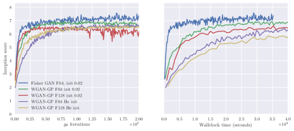
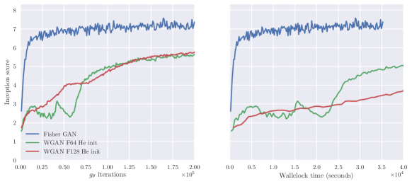
Refer to caption
Figure 6: Architecture and initialization variations, trained with WGAN-GP. Fisher included for comparison. In the main text (Figure 5) we only compare against the best architecture F64 init 0.02.
Refer to caption
Figure 7: Architecture variations, trained with WGAN. Fisher included for comparison.

F.2 LSUN and CelebA.

### LSUN and CelebA: 64x64 dcgan with G_extra_layers=2 and D_extra_layers=0
G (
(main): Sequential (
(0): ConvTranspose2d(100, 512, kernel_size=(4, 4), stride=(1, 1), bias=False)
(1): BatchNorm2d(512, eps=1e-05, momentum=0.1, affine=True)
(2): ReLU (inplace)
(3): ConvTranspose2d(512, 256, kernel_size=(4, 4), stride=(2, 2), padding=(1, 1), bias=False)
(4): BatchNorm2d(256, eps=1e-05, momentum=0.1, affine=True)
(5): ReLU (inplace)
(6): ConvTranspose2d(256, 128, kernel_size=(4, 4), stride=(2, 2), padding=(1, 1), bias=False)
(7): BatchNorm2d(128, eps=1e-05, momentum=0.1, affine=True)
(8): ReLU (inplace)
(9): ConvTranspose2d(128, 64, kernel_size=(4, 4), stride=(2, 2), padding=(1, 1), bias=False)
(10): BatchNorm2d(64, eps=1e-05, momentum=0.1, affine=True)
(11): ReLU (inplace)
(12): Conv2d(64, 64, kernel_size=(3, 3), stride=(1, 1), padding=(1, 1), bias=False)
(13): BatchNorm2d(64, eps=1e-05, momentum=0.1, affine=True)
(14): ReLU (inplace)
(15): Conv2d(64, 64, kernel_size=(3, 3), stride=(1, 1), padding=(1, 1), bias=False)
(16): BatchNorm2d(64, eps=1e-05, momentum=0.1, affine=True)
(17): ReLU (inplace)
(18): ConvTranspose2d(64, 3, kernel_size=(4, 4), stride=(2, 2), padding=(1, 1), bias=False)
(19): Tanh ()
)
)
D (
(main): Sequential (
(0): Conv2d(3, 64, kernel_size=(4, 4), stride=(2, 2), padding=(1, 1), bias=False)
(1): LeakyReLU (0.2, inplace)
(2): Conv2d(64, 128, kernel_size=(4, 4), stride=(2, 2), padding=(1, 1), bias=False)
(3): BatchNorm2d(128, eps=1e-05, momentum=0.1, affine=True)
(4): LeakyReLU (0.2, inplace)
(5): Conv2d(128, 256, kernel_size=(4, 4), stride=(2, 2), padding=(1, 1), bias=False)
(6): BatchNorm2d(256, eps=1e-05, momentum=0.1, affine=True)
(7): LeakyReLU (0.2, inplace)
(8): Conv2d(256, 512, kernel_size=(4, 4), stride=(2, 2), padding=(1, 1), bias=False)
(9): BatchNorm2d(512, eps=1e-05, momentum=0.1, affine=True)
(10): LeakyReLU (0.2, inplace)
)
(V): Linear (8192 -> 1)
)

F.3 CIFAR-10: Sample Quality and Inceptions Scores Experiments

### CIFAR-10: 32x32 dcgan with G_extra_layers=2 and D_extra_layers=2. For samples and inception.
G (
(main): Sequential (
(0): ConvTranspose2d(100, 256, kernel_size=(4, 4), stride=(1, 1), bias=False)
(1): BatchNorm2d(256, eps=1e-05, momentum=0.1, affine=True)
(2): ReLU (inplace)
(3): ConvTranspose2d(256, 128, kernel_size=(4, 4), stride=(2, 2), padding=(1, 1), bias=False)
(4): BatchNorm2d(128, eps=1e-05, momentum=0.1, affine=True)
(5): ReLU (inplace)
(6): ConvTranspose2d(128, 64, kernel_size=(4, 4), stride=(2, 2), padding=(1, 1), bias=False)
(7): BatchNorm2d(64, eps=1e-05, momentum=0.1, affine=True)
(8): ReLU (inplace)
(9): Conv2d(64, 64, kernel_size=(3, 3), stride=(1, 1), padding=(1, 1), bias=False)
(10): BatchNorm2d(64, eps=1e-05, momentum=0.1, affine=True)
(11): ReLU (inplace)
(12): Conv2d(64, 64, kernel_size=(3, 3), stride=(1, 1), padding=(1, 1), bias=False)
(13): BatchNorm2d(64, eps=1e-05, momentum=0.1, affine=True)
(14): ReLU (inplace)
(15): ConvTranspose2d(64, 3, kernel_size=(4, 4), stride=(2, 2), padding=(1, 1), bias=False)
(16): Tanh ()
)
)
D (
(main): Sequential (
(0): Conv2d(3, 64, kernel_size=(4, 4), stride=(2, 2), padding=(1, 1), bias=False)
(1): LeakyReLU (0.2, inplace)
(2): Conv2d(64, 64, kernel_size=(3, 3), stride=(1, 1), padding=(1, 1), bias=False)
(3): BatchNorm2d(64, eps=1e-05, momentum=0.1, affine=True)
(4): LeakyReLU (0.2, inplace)
(5): Conv2d(64, 64, kernel_size=(3, 3), stride=(1, 1), padding=(1, 1), bias=False)
(6): BatchNorm2d(64, eps=1e-05, momentum=0.1, affine=True)
(7): LeakyReLU (0.2, inplace)
(8): Conv2d(64, 128, kernel_size=(4, 4), stride=(2, 2), padding=(1, 1), bias=False)
(9): BatchNorm2d(128, eps=1e-05, momentum=0.1, affine=True)
(10): LeakyReLU (0.2, inplace)
(11): Conv2d(128, 256, kernel_size=(4, 4), stride=(2, 2), padding=(1, 1), bias=False)
(12): BatchNorm2d(256, eps=1e-05, momentum=0.1, affine=True)
(13): LeakyReLU (0.2, inplace)
)
(V): Linear (4096 -> 1)
(S): Linear (6144 -> 10)
)

F.4 CIFAR-10: SSL Experiments

### CIFAR-10: 32x32 D is in the flavor OpenAI Improved GAN, ALI.
G same as above.
D (
(main): Sequential (
(0): Dropout (p = 0.2)
(1): Conv2d(3, 96, kernel_size=(3, 3), stride=(1, 1), padding=(1, 1))
(2): LeakyReLU (0.2, inplace)
(3): Conv2d(96, 96, kernel_size=(3, 3), stride=(1, 1), padding=(1, 1), bias=False)
(4): BatchNorm2d(96, eps=1e-05, momentum=0.1, affine=True)
(5): LeakyReLU (0.2, inplace)
(6): Conv2d(96, 96, kernel_size=(3, 3), stride=(2, 2), padding=(1, 1), bias=False)
(7): BatchNorm2d(96, eps=1e-05, momentum=0.1, affine=True)
(8): LeakyReLU (0.2, inplace)
(9): Dropout (p = 0.5)
(10): Conv2d(96, 192, kernel_size=(3, 3), stride=(1, 1), padding=(1, 1), bias=False)
(11): BatchNorm2d(192, eps=1e-05, momentum=0.1, affine=True)
(12): LeakyReLU (0.2, inplace)
(13): Conv2d(192, 192, kernel_size=(3, 3), stride=(1, 1), padding=(1, 1), bias=False)
(14): BatchNorm2d(192, eps=1e-05, momentum=0.1, affine=True)
(15): LeakyReLU (0.2, inplace)
(16): Conv2d(192, 192, kernel_size=(3, 3), stride=(2, 2), padding=(1, 1), bias=False)
(17): BatchNorm2d(192, eps=1e-05, momentum=0.1, affine=True)
(18): LeakyReLU (0.2, inplace)
(19): Dropout (p = 0.5)
(20): Conv2d(192, 384, kernel_size=(3, 3), stride=(1, 1), bias=False)
(21): BatchNorm2d(384, eps=1e-05, momentum=0.1, affine=True)
(22): LeakyReLU (0.2, inplace)
(23): Dropout (p = 0.5)
(24): Conv2d(384, 384, kernel_size=(3, 3), stride=(1, 1), bias=False)
(25): BatchNorm2d(384, eps=1e-05, momentum=0.1, affine=True)
(26): LeakyReLU (0.2, inplace)
(27): Dropout (p = 0.5)
(28): Conv2d(384, 384, kernel_size=(1, 1), stride=(1, 1), bias=False)
(29): BatchNorm2d(384, eps=1e-05, momentum=0.1, affine=True)
(30): LeakyReLU (0.2, inplace)
(31): Dropout (p = 0.5)
)
(V): Linear (6144 -> 1)
(S): Linear (6144 -> 10)
)

Appendix G Sample implementation in PyTorch

This minimalistic sample code is based on https://github.com/martinarjovsky/WassersteinGAN at commit d92c503.

Some elements that could be added are:

  • Validation loop

  • Monitoring of weights and activations

  • Separate weight decay for last layer v𝑣v (we trained with 1e31e31\mathrm{e}{-3} weight decay on v𝑣v).

  • Adding Cross-Entropy objective and class-conditioned generator.

G.1 Main loop

First note the essential change in the critic’s forward pass definition:

- output = output.mean(0)
- return output.view(1)
+ return output.view(-1)

Then the main training loop becomes:

gen_iterations = 0
for epoch in range(opt.niter):
data_iter = iter(dataloader)
i = 0
while i < len(dataloader):
############################
# (1) Update D network
###########################
for p in netD.parameters(): # reset requires_grad
p.requires_grad = True # they are set to False below in netG update
# train the discriminator Diters times
if opt.hiDiterStart and (gen_iterations < 25 or gen_iterations % 500 == 0):
Diters = 100
else:
Diters = opt.Diters
j = 0
while j < Diters and i < len(dataloader):
j += 1
data = data_iter.next()
i += 1
# train with real
real_cpu, _ = data
netD.zero_grad()
batch_size = real_cpu.size(0)
if opt.cuda:
real_cpu = real_cpu.cuda()
input.resize_as_(real_cpu).copy_(real_cpu)
inputv = Variable(input)
vphi_real = netD(inputv)
# train with fake
noise.resize_(opt.batchSize, nz, 1, 1).normal_(0, 1)
noisev = Variable(noise, volatile = True) # totally freeze netG
fake = Variable(netG(noisev).data)
inputv = fake
vphi_fake = netD(inputv)
# NOTE here f = <v,phi> , but with modified f the below two lines are the
# only ones that need change. E_P and E_Q refer to Expectation over real and fake.
E_P_f, E_Q_f = vphi_real.mean(), vphi_fake.mean()
E_P_f2, E_Q_f2 = (vphi_real**2).mean(), (vphi_fake**2).mean()
constraint = (1 - (0.5*E_P_f2 + 0.5*E_Q_f2))
# See Equation (9)
obj_D = E_P_f - E_Q_f + alpha * constraint - opt.rho/2 * constraint**2
# max_w min_alpha obj_D. Compute negative gradients, apply updates with negative sign.
obj_D.backward(mone)
optimizerD.step()
# artisanal sgd. We minimze alpha so a <- a + lr * (-grad)
alpha.data += opt.rho * alpha.grad.data
alpha.grad.data.zero_()
############################
# (2) Update G network
###########################
for p in netD.parameters():
p.requires_grad = False # to avoid computation
netG.zero_grad()
# in case our last batch was the tail batch of the dataloader,
# make sure we feed a full batch of noise
noise.resize_(opt.batchSize, nz, 1, 1).normal_(0, 1)
noisev = Variable(noise)
fake = netG(noisev)
vphi_fake = netD(fake)
obj_G = -vphi_fake.mean() # Just minimize mean difference
obj_G.backward() # G: min_theta
optimizerG.step()
gen_iterations += 1

G.2 Full diff from reference

Note that from the arXiv   source, the file diff.txt could be used in combination with git apply.

diff --git a/main.py b/main.py
index 7c3e638..e0cae42 100644
--- a/main.py
+++ b/main.py
@@ -34,15 +34,17 @@ parser.add_argument(’--cuda’ , action=’store_true’, help=’enables cuda’)
parser.add_argument(’--ngpu’ , type=int, default=1, help=’number of GPUs to use’)
parser.add_argument(’--netG’, default=’’, help="path to netG (to continue training)")
parser.add_argument(’--netD’, default=’’, help="path to netD (to continue training)")
-parser.add_argument(’--clamp_lower’, type=float, default=-0.01)
-parser.add_argument(’--clamp_upper’, type=float, default=0.01)
+parser.add_argument(’--wdecay’, type=float, default=0.000, help=’wdecay value for Phi’)
parser.add_argument(’--Diters’, type=int, default=5, help=’number of D iters per each G iter’)
+parser.add_argument(’--hiDiterStart’ , action=’store_true’, help=’do many D iters at start’)
parser.add_argument(’--noBN’, action=’store_true’, help=’use batchnorm or not (only for DCGAN)’)
parser.add_argument(’--mlp_G’, action=’store_true’, help=’use MLP for G’)
parser.add_argument(’--mlp_D’, action=’store_true’, help=’use MLP for D’)
-parser.add_argument(’--n_extra_layers’, type=int, default=0, help=’Number of extra layers on gen and disc’)
+parser.add_argument(’--G_extra_layers’, type=int, default=0, help=’Number of extra layers on gen and disc’)
+parser.add_argument(’--D_extra_layers’, type=int, default=0, help=’Number of extra layers on gen and disc’)
parser.add_argument(’--experiment’, default=None, help=’Where to store samples and models’)
parser.add_argument(’--adam’, action=’store_true’, help=’Whether to use adam (default is rmsprop)’)
+parser.add_argument(’--rho’, type=float, default=1e-6, help=’Weight on the penalty term for (sigmas -1)**2’)
opt = parser.parse_args()
print(opt)
@@ -60,7 +62,7 @@ cudnn.benchmark = True
if torch.cuda.is_available() and not opt.cuda:
print("WARNING: You have a CUDA device, so you should probably run with --cuda")
-if opt.dataset in [’imagenet’, ’folder’, ’lfw’]:
+if opt.dataset in [’imagenet’, ’folder’, ’lfw’, ’celeba’]:
# folder dataset
dataset = dset.ImageFolder(root=opt.dataroot,
transform=transforms.Compose([
@@ -94,7 +96,6 @@ nz = int(opt.nz)
ngf = int(opt.ngf)
ndf = int(opt.ndf)
nc = int(opt.nc)
-n_extra_layers = int(opt.n_extra_layers)
# custom weights initialization called on netG and netD
def weights_init(m):
@@ -106,11 +107,11 @@ def weights_init(m):
m.bias.data.fill_(0)
if opt.noBN:
- netG = dcgan.DCGAN_G_nobn(opt.imageSize, nz, nc, ngf, ngpu, n_extra_layers)
+ netG = dcgan.DCGAN_G_nobn(opt.imageSize, nz, nc, ngf, ngpu, opt.G_extra_layers)
elif opt.mlp_G:
netG = mlp.MLP_G(opt.imageSize, nz, nc, ngf, ngpu)
else:
- netG = dcgan.DCGAN_G(opt.imageSize, nz, nc, ngf, ngpu, n_extra_layers)
+ netG = dcgan.DCGAN_G(opt.imageSize, nz, nc, ngf, ngpu, opt.G_extra_layers)
netG.apply(weights_init)
if opt.netG != ’’: # load checkpoint if needed
@@ -120,7 +121,7 @@ print(netG)
if opt.mlp_D:
netD = mlp.MLP_D(opt.imageSize, nz, nc, ndf, ngpu)
else:
- netD = dcgan.DCGAN_D(opt.imageSize, nz, nc, ndf, ngpu, n_extra_layers)
+ netD = dcgan.DCGAN_D(opt.imageSize, nz, nc, ndf, ngpu, opt.D_extra_layers)
netD.apply(weights_init)
if opt.netD != ’’:
@@ -132,6 +133,7 @@ noise = torch.FloatTensor(opt.batchSize, nz, 1, 1)
fixed_noise = torch.FloatTensor(opt.batchSize, nz, 1, 1).normal_(0, 1)
one = torch.FloatTensor([1])
mone = one * -1
+alpha = torch.FloatTensor([0]) # lagrange multipliers
if opt.cuda:
netD.cuda()
@@ -139,14 +141,16 @@ if opt.cuda:
input = input.cuda()
one, mone = one.cuda(), mone.cuda()
noise, fixed_noise = noise.cuda(), fixed_noise.cuda()
+ alpha = alpha.cuda()
+alpha = Variable(alpha, requires_grad=True)
# setup optimizer
if opt.adam:
- optimizerD = optim.Adam(netD.parameters(), lr=opt.lrD, betas=(opt.beta1, 0.999))
- optimizerG = optim.Adam(netG.parameters(), lr=opt.lrG, betas=(opt.beta1, 0.999))
+ optimizerD = optim.Adam(netD.parameters(), lr=opt.lrD, betas=(opt.beta1, 0.999), weight_decay=opt.wdecay)
+ optimizerG = optim.Adam(netG.parameters(), lr=opt.lrG, betas=(opt.beta1, 0.999), weight_decay=opt.wdecay)
else:
- optimizerD = optim.RMSprop(netD.parameters(), lr = opt.lrD)
- optimizerG = optim.RMSprop(netG.parameters(), lr = opt.lrG)
+ optimizerD = optim.RMSprop(netD.parameters(), lr = opt.lrD, weight_decay=opt.wdecay)
+ optimizerG = optim.RMSprop(netG.parameters(), lr = opt.lrG, weight_decay=opt.wdecay)
gen_iterations = 0
for epoch in range(opt.niter):
@@ -160,7 +164,7 @@ for epoch in range(opt.niter):
p.requires_grad = True # they are set to False below in netG update
# train the discriminator Diters times
- if gen_iterations < 25 or gen_iterations % 500 == 0:
+ if opt.hiDiterStart and (gen_iterations < 25 or gen_iterations % 500 == 0):
Diters = 100
else:
Diters = opt.Diters
@@ -168,10 +172,6 @@ for epoch in range(opt.niter):
while j < Diters and i < len(dataloader):
j += 1
- # clamp parameters to a cube
- for p in netD.parameters():
- p.data.clamp_(opt.clamp_lower, opt.clamp_upper)
-
data = data_iter.next()
i += 1
@@ -185,18 +185,28 @@ for epoch in range(opt.niter):
input.resize_as_(real_cpu).copy_(real_cpu)
inputv = Variable(input)
- errD_real = netD(inputv)
- errD_real.backward(one)
+ vphi_real = netD(inputv)
# train with fake
noise.resize_(opt.batchSize, nz, 1, 1).normal_(0, 1)
noisev = Variable(noise, volatile = True) # totally freeze netG
fake = Variable(netG(noisev).data)
inputv = fake
- errD_fake = netD(inputv)
- errD_fake.backward(mone)
- errD = errD_real - errD_fake
+
+ vphi_fake = netD(inputv)
+ # NOTE here f = <v,phi> , but with modified f the below two lines are the
+ # only ones that need change. E_P and E_Q refer to Expectation over real and fake.
+ E_P_f, E_Q_f = vphi_real.mean(), vphi_fake.mean()
+ E_P_f2, E_Q_f2 = (vphi_real**2).mean(), (vphi_fake**2).mean()
+ constraint = (1 - (0.5*E_P_f2 + 0.5*E_Q_f2))
+ # See Equation (9)
+ obj_D = E_P_f - E_Q_f + alpha * constraint - opt.rho/2 * constraint**2
+ # max_w min_alpha obj_D. Compute negative gradients, apply updates with negative sign.
+ obj_D.backward(mone)
optimizerD.step()
+ # artisanal sgd. We minimze alpha so a <- a + lr * (-grad)
+ alpha.data += opt.rho * alpha.grad.data
+ alpha.grad.data.zero_()
############################
# (2) Update G network
@@ -209,14 +219,20 @@ for epoch in range(opt.niter):
noise.resize_(opt.batchSize, nz, 1, 1).normal_(0, 1)
noisev = Variable(noise)
fake = netG(noisev)
- errG = netD(fake)
- errG.backward(one)
+ vphi_fake = netD(fake)
+ obj_G = -vphi_fake.mean() # Just minimize mean difference
+ obj_G.backward() # G: min_theta
optimizerG.step()
gen_iterations += 1
- print(’[%d/%d][%d/%d][%d] Loss_D: %f Loss_G: %f Loss_D_real: %f Loss_D_fake %f’
+ IPM_enum = E_P_f.data[0] - E_Q_f.data[0]
+ IPM_denom = (0.5*E_P_f2.data[0] + 0.5*E_Q_f2.data[0]) ** 0.5
+ IPM_ratio = IPM_enum / IPM_denom
+ print((’[%d/%d][%d/%d][%d] IPM_enum: %.4f IPM_denom: %.4f IPM_ratio: %.4f
+ ’E_P_f: %.4f E_Q_f: %.4f E_P_(f^2): %.4f E_Q_(f^2): %.4f’)
% (epoch, opt.niter, i, len(dataloader), gen_iterations,
- errD.data[0], errG.data[0], errD_real.data[0], errD_fake.data[0]))
+ IPM_enum, IPM_denom, IPM_ratio,
+ E_P_f.data[0], E_Q_f.data[0], E_P_f2.data[0], E_Q_f2.data[0]))
if gen_iterations % 500 == 0:
real_cpu = real_cpu.mul(0.5).add(0.5)
vutils.save_image(real_cpu, ’{0}/real_samples.png’.format(opt.experiment))
diff --git a/models/dcgan.py b/models/dcgan.py
index 1dd8dbf..ea86a94 100644
--- a/models/dcgan.py
+++ b/models/dcgan.py
@@ -48,9 +48,7 @@ class DCGAN_D(nn.Module):
output = nn.parallel.data_parallel(self.main, input, range(self.ngpu))
else:
output = self.main(input)
-
- output = output.mean(0)
- return output.view(1)
+ return output.view(-1)
class DCGAN_G(nn.Module):
def __init__(self, isize, nz, nc, ngf, ngpu, n_extra_layers=0):
@@ -148,9 +146,7 @@ class DCGAN_D_nobn(nn.Module):
output = nn.parallel.data_parallel(self.main, input, range(self.ngpu))
else:
output = self.main(input)
-
- output = output.mean(0)
- return output.view(1)
+ return output.view(-1)
class DCGAN_G_nobn(nn.Module):
def __init__(self, isize, nz, nc, ngf, ngpu, n_extra_layers=0):