Microlensing constraints on primordial black holes with the Subaru/HSC Andromeda observation

Abstract

Primordial black holes (PBHs) have long been suggested as a viable candidate for the elusive dark matter (DM). The abundance of such PBHs has been constrained using a number of astrophysical observations, except for a hitherto unexplored mass window of $M_{\rm PBH}=[10^{-14},10^{-9}]M_{\odot}$. Here we carry out a dense-cadence (2 min sampling rate), 7 hour-long observation of the Andromeda galaxy (M31) with the Subaru Hyper Suprime-Cam to search for microlensing of stars in M31 by PBHs lying in the halo regions of the Milky Way (MW) and M31. Given our simultaneous monitoring of more than tens of millions of stars in M31, if such light PBHs make up a significant fraction of DM, we expect to find many microlensing events for the PBH DM scenario. However, we identify only a single candidate event, which translates into the most stringent upper bounds on the abundance of PBHs in the mass range $M_{\rm PBH}\simeq[10^{-11},10^{-6}]M_{\odot}$.

Hiroko Niikura^1,2, Masahiro Takada¹, Naoki Yasuda¹, Robert H. Lupton³, Takahiro Sumi⁴, Surhud More¹, Toshiki Kurita^1,2, Sunao Sugiyama^1,2, Anupreeta More¹, Masamune Oguri^1,2,5, Masashi Chiba⁶

• Kavli Institute for the Physics and Mathematics of the Universe (WPI), The University of Tokyo Institutes for Advanced Study (UTIAS), The University of Tokyo, Chiba, 277-8583, Japan

• Physics Department, The University of Tokyo, Bunkyo, Tokyo 113-0031, Japan

• Department of Astrophysical Sciences, Princeton University, Peyton Hall, Princeton NJ 08544 USA

• Department of Earth and Space Science, Graduate School of Science, Osaka University, Toyonaka, Osaka 560-0043, Japan

• Research Center for the Early Universe, University of Tokyo, Tokyo 113-0033, Japan

• Astronomical Institute, Tohoku University, Aoba-ku, Sendai 980-8578, Japan

The nature of dark matter (DM) remains one of the most important problems in physics. Previous studies have suggested that DM is non-baryonic, non-relativistic, and interacts with ordinary matter only via gravity [1, 2, 3]. Currently, unknown stable particle(s) beyond the Standard Model of Particle Physics, such as Weakly Interacting Massive Particles (WIMPs), are considered to be viable candidates [4]. However such particles have so far evaded detection in either elastic scattering experiments, indirect experiments or collider experiments [5]. Primordial black holes (PBH), which can be formed during the early universe, are also viable candidates for the elusive DM [6, 7, 8].

Figure 1: The background shows the HSC image of M31 as seen by the 104 CCD chips of the Subaru/HSC camera. The white-colored grid represents a predefined iso-latitude tessellation grid, called the HSC “patch” (approximately 12 arcmin on a side). Our data analysis including the image subtraction is performed on individual patches. We exclude those patches which are marked in dark-blue color from our analysis as the dense star fields in these patches result in a saturation of the CCDs.

Figure 2: The expected differential number of PBH microlensing events per logarithmic interval of the full-width-at-half-maximum (FWHM) microlensing timescale ${t_{\rm FWHM}}$, for a single star in M31. Each solid line corresponds to a monochromatic PBH DM scenario and assumes that all the dark matter consists of such PBHs. We adopt DM halo models for the MW and M31 halos which reproduce their individual rotation curves. The event rate calculation includes distributions of impact parameters and velocities of PBHs relative to a source star. Given the cadence, our data has the highest sensitivity to measure lightcurves with $t_{\rm FWHM}\simeq[0.07,3]~{}{\rm hours}$ shown by the unshaded regions.

The abundance of PBHs of different mass scales is already constrained by various observations except for a mass window of $M_{\rm PBH}\simeq[10^{19},10^{24}]$g or equivalently $[10^{-14},10^{-9}]M_{\odot}$ [9]. The existing constraints based on the capture of neutron stars and white dwarfs [10] in this mass regime are based on uncertain assumptions about the presence of DM in a globular cluster [11]. Thus it is of critical importance to further explore observational constraints on the PBH abundance for this mass window.

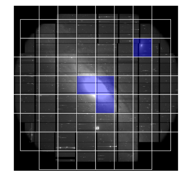
Gravitational microlensing is a powerful method to probe DM in the Milky Way (MW) [12, 13]. Microlensing causes a time-varying magnification of a background star when a lensing object crosses the line-of-sight to the star at close proximity. The microlensing experiments, MACHO [14] and EROS [15], have previously monitored large number of stars in the Large Magellanic Cloud (LMC) with roughly a 24 hour cadence. They have ruled out massive compact halo objects (MACHOs) such as brown dwarfs with mass scales $[10^{-7},10]M_{\odot}$ as DM candidates. We also note that if PBHs with mass around $10M_{\odot}$ comprise even 1% of the DM and form binaries, then their merger rate could be larger than the LIGO event rate [16, 17]. Microlensing searches on time scales of 15 or 30 minutes have also been carried out using the public 2-year Kepler data to constrain the abundance of $10^{-8}M_{\odot}$ PBHs [18]. With the aim of constraining the abundance of PBH on even smaller mass scales, we carried out a dense cadence observation of the Andromeda galaxy (M31), with the Subaru Hyper Suprime-Cam (HSC). We search for microlensing event(s) of M31 stars by intervening PBHs in both the halo regions of MW and M31. M31 is the MW’s largest neighboring spiral galaxy, at a distance of 770 kpc (the distance modulus $\mu\simeq 24.4~{}$mag). Even a single night of HSC/Subaru yields an ideal dataset to search for the PBH microlensing events for the following reasons. First, the 1.5 degree diameter field-of-view of HSC [19] allows us to cover the entire region of M31 (the bulge, disk and halo regions) with a single pointing, as shown in Fig. 1. Secondly, the 8.2m large aperture and its superb image quality (typically $0.6^{\prime\prime}$ seeing)[20] allow us to detect fluxes from M31 stars down to $m_{r}\simeq 26$ even with a short exposure of 90 sec. These two facts allow us to simultaneously monitor a sufficiently large number of stars in M31. Thirdly, the 90 sec exposure and a short camera readout of $\sim$35 sec enable us to take data at an unprecedented cadence of 2 min. Thus, we can search for microlensing events with PBH mass scales smaller than those probed by Ref. [18]. Finally, the huge volume between M31 and the Earth, leads to a large optical depth of PBH microlensing to each star in M31, which allows us to put meaningful constraints on the PBH DM scenario.

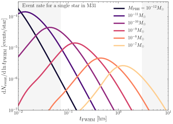
In Fig. 2 we show the differential number of PBH microlensing events for a single star in M31 per logarithmic timescale, for our 7 hour-long HSC observation, assuming that PBHs of a single mass scale make up all DM in the halo regions of MW and M31. Here we consider a monochromatic PBH mass-scale for illustrative purposes. However, our limits will apply to a general scenario of PBH DM with an arbitrary mass spectrum. To model the DM distribution, we adopt the halo model for the MW and M31 from Ref. [21], with model parameters constrained by the observed galaxy rotation curves. We assume $M_{\rm vir}=10^{12}M_{\odot}$ and $1.6\times 10^{12}M_{\odot}$ as the virial mass of the MW and the M31 halo, respectively. To be conservative, we ignore any further DM contribution arising in the intervening space between MW and M31, e.g. due to a possible filamentary structure between the two galaxies. Once the halo model parameters, the distance to the lensing PBH, the impact parameter and the tangential velocity relative to the source star on the sky, are specified, we can predict the microlensing light curve. Different combinations of the model parameters could produce a similar timescale for the light curve. The expected event number in Fig. 2 takes into account variations of the parameters, by integrating the differential event rate over the ranges of model parameters for a fixed PBH mass and a fixed microlensing timescale. Throughout this paper we characterize each microlensing light curve by its full-width-at-half-maximum (FWHM) timescale, $t_{\rm FWHM}$. The constraint on the abundance of PBHs can be obtained by integrating the expected microlensing events over all possible light-curve timescales accessible to our observations. Our dense HSC data is most sensitive to light curves with timescales ranging from a few minutes to a few hours. The expected number of PBH microlensing is quite high, up to $\mathrm{d}N_{\rm exp}/\mathrm{d}\ln t_{\rm FWHM}\sim 10^{-5}$ for a light curve timescale of $t_{\rm FWHM}\sim 0.1~{}$hours. Hence, if we monitor $10^{8}$ stars in M31 with each exposure (visit) as we will describe below, we can expect to observe $\sim 10^{3}$ events if such PBHs constitute most DM in the MW and M31 halo regions. Since a PBH in the halo region has a typical motion of 200 ${\rm km}/{\rm s}$ as implied by the rotation curve irrespectively of PBH mass, a lighter PBH will result in an event with a shorter timescale, owing to its smaller Einstein radius. This makes high-cadence observations of M31 ideally suited for the search of microlensing events arising from lighter PBHs.

Figure 3: An example of the image subtraction technique we use for the analysis in this paper. The left panel shows the reference image which was constructed by co-adding the images of 10 best-seeing epochs, with a typical seeing of $0.45^{\prime\prime}$. The size of the image is $222\times 356$ pixels (corresponding to about 0.63 sq. arcmin), and corresponds to the disk region in M31. The middle panel shows a target image (coadded image using 3 sequential exposures) with seeing size of $0.8^{\prime\prime}$. The right panel shows the difference image generated by our image subtraction pipeline properly accounting for the different seeing of the target and reference images even in such a densely populated stellar field. A variable star candidate shows up in the difference image at the center. In this case, the candidate object appears as a negative flux in the difference image, because the object was fainter in the target image than in the reference image.

Motivated by these considerations, we carried out a dense-cadence HSC observation of M31 in the $r$-band on the night of November 23, 2014. The HSC camera has 104 science detectors with a pixel scale of $0.168^{\prime\prime}$ [19, 22] (see Fig. 1). The pointing was centered at the coordinates of the M31 central region: (RA, dec) = (00h 42m 44.420s,+41d 16m 10.1s). We did not adopt any dithering (moving the pointing directions) between different exposures in order to keep the same stars in the same CCD chip. We carried out the observations with a cadence of 2 minutes, and acquired 194 exposures for M31 during 7 hours within the same night until the elevation of M31 fell below about $30$ degrees. The last 6 of the exposures at the end of our observations suffered from bad seeing, $\lower 2.15277pt\hbox{$\;\buildrel>\over{\sim}\;$}1.2^{\prime\prime}$. Therefore in our analysis, we use 188 exposures in total. These data yield a densely-sampled light curve for every variable star candidate in the field with a 2-min cadence.

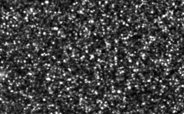
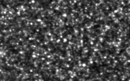
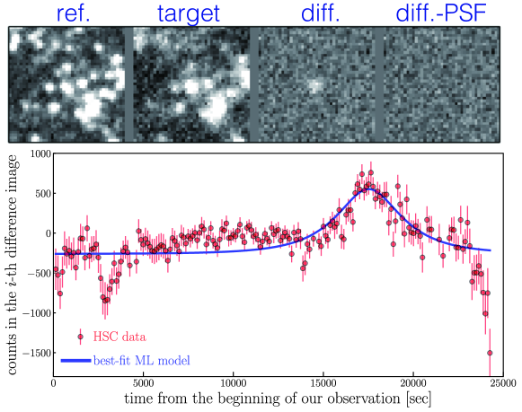
The analysis of M31 time domain data presents a formidable challenge, as it is a dense stellar field. We are in the pixel lensing regime, where we need to detect the microlensing of a single unresolved star among many stars that contribute photons to each CCD pixel [23, 24, 25]. All of the previous work on M31 microlensing (e.g., see [26]) has been carried out using smaller aperture telescopes, which can only be sensitive to microlensing of relatively bright stars such as red giants [27]. In addition the image quality of HSC corresponds to a significant step ahead, especially given the typical seeing size $\sim 0.6^{\prime\prime}$. In order to search for pixel lensing, we used the image subtraction technique described in Alard & Lupton [28]. This technique has been integrated into the standard HSC data reduction pipeline, $\mathtt{hscPipe}$ [29]. The pipeline subtracts a reference image (constructed from the 10 epochs with the best seeing data) from a target image for M31 taken at a different epoch, and catalogs variable star candidates that are identified in the difference image. In Fig. 3, we demonstrate an example of the image difference technique successfully performed by our pipeline in a typically dense stellar field in M31. A variable star candidate, which undergoes a flux change between the reference and target epochs, appears in the difference image, as shown in the right panel. We exclude the core bulge of M31 and the region including M101 from our analysis where there are many saturated stars as there is no hope of recovering microlensing events buried in saturated pixels even with an image difference technique.

Figure 4: The single remaining candidate that passed all the criteria we impose to select microlensing events. The images in the upper panels show the postage-stamped images around the candidate: the reference image, the target image, the difference image and the residual image after subtracting the best-fit PSF image, respectively. The lower panel shows that the best-fit microlensing model (blue curve) gives an acceptable fit to the measured light curve. The error bars denote photometric errors in the brightness measurement in the different image at each epoch.

We extract 15571 candidate variable stars, from the difference images constructed by subtracting the reference image from each of the 188 target images. All of these candidates satisfy our basic selection criteria – (a) at least a $5\sigma$ detection of flux in any of the 188 difference images, and (b) the difference image of the candidate is consistent with the Point Spread Function (PSF). Subsequently, we perform PSF photometry at the center of each candidate in all of the difference images. This allows us to measure the light curve of the candidate as a function of time, sampled every 2 min, through our 7 hour-long observation period. Our candidates include many secure detections of variable events such as stellar flares, eclipsing contact binaries and Cepheid variables. However, our photometry comes with an important caveat. The photometry in the difference image measures only the flux change between the reference and target images. Although we also use the PSF photometry at the candidate position in the reference image to infer the intrinsic flux of the candidate star, this photometry could be contaminated by fluxes of neighboring stars. Among the 15,571 variables we detect, about 3000 are brighter than $m_{r}=25$, while the rest extend down to $m_{r}\sim 26$. Thus, even with a 90 sec short exposure, the 8.2 m aperture and excellent image quality enables us to detect variables stars down to $m_{r}\sim 25$–$26$, which clearly shows the power of HSC/Subaru for time domain astronomy.

We then search for microlensing events from our master catalog of 15,571 variable star candidates. As the optical depth of microlensing towards a single star is $\tau\ll 1$, the probability to have multiple lensing events for the same source star is negligible. Therefore, we impose a level 1 requirement that a candidate should have a single “bump” feature in the light curve, defined by 3 time-consecutive flux changes each with a significance greater than $5\sigma$ in the difference image. This selection leaves us with $11,703$ candidates. Then we fit the parameters of a microlensing model with each measured light curve. The microlensing light curve in the difference images is characterized by 3 parameters: the impact parameter, the light-curve FWHM timescale and the intrinsic flux (more exactly the intrinsic ADU counts of the candidate in the difference image). To perform a $\chi^{2}$-fit to the data, we estimate the rms noise of PSF photometry in each of the difference images by estimating the PSF photometry at 1,000 random points in each HSC patch region (see Fig. 1). We keep only those candidates which yield a best fit reduced $\chi$-squared value, $\chi^{2}_{\rm best-fit}/185<3.5$ (the degrees of freedom are $185=188-3$). This criterion is sufficiently conservative (the P-value is $\sim 10^{-5}$) for us not to miss a real microlensing candidate, if it exists. We further impose the condition that the light curve has a symmetric shape around the peak. These selections leave us with a total of 66 candidates.

Finally we perform a visual inspection of each of the remaining candidates. We found various impostors that are not removed by the above automated criteria. Most of them are a result of imperfect image subtraction; in most cases the difference image has significant residuals near the edges of CCD chip or around a bright star. In particular, bright stars cause a spiky residual in the difference image, which result in impostors with a microlensing-like light curve if the PSF flux is measured at a fixed position. We found 44 such impostors which were a result of such spike-like images around bright stars. Of the remaining, 20 impostors were located at the edges of the CCDs. We also identified 1 impostor event caused by a moving object, an asteroid. If the light curve is measured at a fixed position where the asteroid passes, it results in a light curve which mimics microlensing. In summary, the visual inspection left us with a single candidate which passed all our cuts and visual checks. The candidate position is $({\rm RA},{\rm dec})=(00{\rm h}~{}45{\rm m}~{}33.413{\rm s},+41{\rm d}~{}07{\rm m}~{}53.03{\rm s})$. Fig. 4 shows the images and the light curve for the remaining candidate. Although the light curve looks noisy, it is consistent with the microlensing prediction. The magnitude of the star inferred from the reference image $m_{r}\sim 24.5$. Unfortunately, the candidate is placed just outside the survey regions of the Panchromatic Hubble Andromeda Treasury (PHAT) catalog in Refs. [30, 31], so the HST image at this location is not available. To address whether the candidate is a variable star, we looked into the $r$-band data that was taken during the HSC commissioning run in 2013, a different epoch from our observing night. If our candidate is a variable star, it would display a time variability at the different epoch. However, the $r$-band commissioning image was unfortunately taken with a seeing of about $1.2^{\prime\prime}$, so the difference image at the candidate position appears noisy. Similarly, we also analyzed the $g$-band images taken during the HSC commissioning run. However, due to the short duration of the data itself ($\sim 15~{}$min), it is difficult to judge whether this candidate has any time variability between the $g$ band images. Therefore, we cannot conclusively infer the nature of this candidate. In what follows, we derive an upper bound on the abundance of PBHs as a constituent of DM assuming that this remaining candidate is real.

Figure 5: The red shaded region corresponds to the 95% C.L. upper bound on the PBH mass fraction to DM in the halo regions of MW and M31, derived from our search for microlensing of M31 stars based on the “single-night” HSC/Subaru data and fills a large gap in the existing constraints by closing the PBH DM window around lunar mass scale. To derive this constraint, we took into account the effect of finite source size, assuming that all source stars in M31 have a solar radius, as well as the effect of wave optics in the HSC $r$-band filter on the microlensing event (see text for details). The effects weaken the upper bounds at $M\lower 2.15277pt\hbox{$\;\buildrel<\over{\sim}\;$}10^{-7}M_{\odot}$, and give no constraint on PBH at $M\lower 2.15277pt\hbox{$\;\buildrel<\over{\sim}\;$}10^{-11}M_{\odot}$. Our constraint can be compared with other observational constraints as shown by the gray shaded regions: extragalactic $\gamma$-rays from PBH evaporation [32], femtolensing of $\gamma$-ray burst (“Femto”) [33], microlensing search of stars from the satellite 2-years Kepler data (“Kepler”) [18], MACHO/EROS/OGLE microlensing of stars (“EROS/MACHO”) [15], and the accretion effects on the CMB observables (“CMB”) [34], updated from the earlier estimate [35].

Now we use the results of our microlensing search to constrain the abundance of PBHs in the halo regions of MW and M31. The expected number of PBH microlensing events in our HSC data is given by

$$N_{\rm exp}\!\left(M_{\rm PBH},\frac{\Omega_{\rm PBH}}{\Omega_{\rm DM}}\right)=\frac{\Omega_{\rm PBH}}{\Omega_{\rm DM}}\int_{0}^{t_{\rm obs}}\!\!\frac{\mathrm{d}t_{\rm FWHM}}{t_{\rm FWHM}}~{}\int\!\!\mathrm{d}m_{r}~{}\frac{\mathrm{d}N_{\rm event}}{\mathrm{d}{\ln t}_{\rm FWHM}}\frac{\mathrm{d}N_{s}}{\mathrm{d}m_{r}}\epsilon({t}_{\rm FWHM},m_{r}),$$ (1)

where $\mathrm{d}N_{\rm exp}/\mathrm{d}t_{\rm FWHM}$ is the differential event rate for a single star (Fig. 2) per logarithmic timescale, $\mathrm{d}{N}/\mathrm{d}m_{r}$ is the luminosity function of source stars in the $r$-band magnitude range $[m_{r},m_{r}+\mathrm{d}m_{r}]$, and $\epsilon(m_{\rm FWHM},m_{r})$ is the detection efficiency quantifying the probability that a microlensing event for a star with magnitude $m_{r}$ and the light curve timescale $t_{\rm FWHM}$ is detected by our selection procedures. The event rate depends on the mass fraction of PBHs to the total DM mass in the halo regions, $\Omega_{\rm PBH}/\Omega_{\rm DM}$. Note that we have assumed a parametric model for the total matter content of the MW and M31 halos constrained by their respective rotation curves (see the explanation for Fig. 2). The PBH DM mass fraction does not depend on the cosmological matter parameter, $\Omega_{\rm m0}$, that is relevant for the cosmic expansion.

We use the following procedure to estimate $\mathrm{d}N_{s}/\mathrm{d}m_{r}$ and $\epsilon$ in Eq. (1). Since individual stars are not resolved in the HSC data, especially in the disk region of M31, it is not straightforward to estimate the number of source stars from the HSC data alone. This constitutes a significant uncertainty in our results. One way to estimate the number of source stars from the HSC data itself is using the number of “detected peaks” in the reference image (the best-seeing co-added image). This estimate is very conservative as it misses the numerous faint stars that do not produce prominent peaks. To overcome this difficulty, we use the HST PHAT star catalog as follows. Our HSC data has an overlap with the HST PHAT survey for the M31 disk region, where individual stars are resolved thanks to the high angular resolution of the ACS/HST data. We found that the number counts of peaks in the HSC image fairly well agrees with the counts in the PHAT catalog down to $m_{r}\sim 23$, after applying a color transformation between the HSC and HST filters, but indeed misses stars at the fainter magnitudes. For the overlapping regions, we used the PHAT star counts down to $m_{r}\sim 26$. For the non-overlapping regions in the M31 disk, we infer the luminosity function by extrapolating the number counts of HSC peaks at $m_{r}=23$ down to $m_{r}=26$ based on the PHAT luminosity function of stars at a similar distance from the M31 center. For our default analysis, we used about $8.7\times 10^{7}$ stars down to $m_{r}=26~{}$mag over the entire region of M31, which is a factor 14 more number of stars than that of HSC peaks. The large number of source stars in the M31 region can be compared with those in previous studies, e.g., [18] used $\sim 1.5\times 10^{5}$ source stars for the microlensing search in Kepler data.

For an estimation of the detection efficiency $\epsilon(t_{\rm FWHM},m_{r})$ in Eq. (1), we carry out Monte Carlo simulations of microlensing light curves adopting random combinations of the model parameters (the impact parameter, $t_{\rm FWHM}$, and the intrinsic flux) and adding the statistical noise based on the photometry errors in each HSC-patch region. These simulations allow us to estimate the fraction of simulated light curves that can be recovered by our selection procedures. As a cross-check, we also use SynPipe [36], a pipeline to inject a synthesized microlensed star into every individual HSC exposure image at a randomly-selected location. We then test whether our microlensing search can identify such synthesized events from these images in order to estimate the detection efficiency. The two methods give similar estimates for the detection efficiency. Our results indicate that our pipeline can recover about 70–60% of microlensing events for stars with intrinsic magnitude $m_{r}=23$–$24~{}$mag, if the timescale is in the range $t_{\rm FWHM}\simeq[0.1,3]~{}{\rm hours}$. For fainter stars with $m_{r}=25~{}$–26 mag, the efficiency is reduced to about 30–20%.

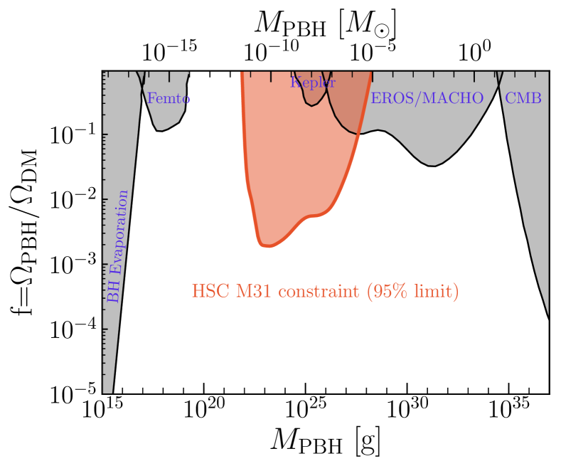
Next we combine the estimates of $\mathrm{dN}_{\rm event}/\mathrm{d}\ln t_{\rm FWHM}$, $\mathrm{d}N_{s}/\mathrm{d}m_{r}$ and $\epsilon(t_{\rm FWHM},m_{r})$ in Eq. (1) to constrain the abundance of PBHs. Assuming the number of microlensing events follow a Poisson distribution, the probability to observe a given number of such events, $N_{\rm obs}$, is given by $P(k=N_{\rm obs}|N_{\rm exp})=\left[\left(N_{\rm exp}\right)^{k}/k!\right]\exp[-N_{\rm exp}]$. Hence the 95% C.L. interval is estimated as $P(k=0)+P(k=1)\geq 0.05$, leading to $N_{\rm exp}\leq 4.74$ assuming that the candidate in Fig. 4 is real. Fig. 5 shows our result in comparison with other observational constraints on the abundance of PBHs on different mass scales. In the results, we took into account the effect of finite source star size [37] as well as the effect of wave optics on the microlensing cross section [38, 39]. The finite-source size results in the magnification of only a small part of the star and hence affects the detectability of the event. The effect modifies our constraints on mass scales, $M_{\rm PBH}\lower 2.15277pt\hbox{$\;\buildrel<\over{\sim}\;$}10^{-7}M_{\odot}$ where the Einstein radii of the PBHs become comparable to or smaller than the size of the source stars. We caution that we may have underestimated the impact somewhat as we have assumed a solar radius for all stars in M31, while some of the stars would likely be giants. The wave effect arises from the fact that the Schwarzschild radii of light PBHs with $M\lower 2.15277pt\hbox{$\;\buildrel<\over{\sim}\;$}10^{-11}M_{\odot}$ become comparable to the wavelength of the HSC $r$-band filter (centered around 600 nm). In this regime, the wave nature of light becomes important and can further lower the maximum magnification of the microlensing light curve. This results in a lower event rate for a given detection threshold. These effects need to be further studied and carefully accounted for. Nevertheless the figure shows that a single night of HSC data on M31 results in a tight upper bound on the mass fraction of PBHs to DM, $\Omega_{\rm PBH}/\Omega_{\rm DM}$. The origin of the constraint can be easily understood. Given that we monitor about $10^{8}$ stars, we expected to observe about 1,000 microlensing events if PBHs of a single mass scale $M_{\rm PBH}\sim 10^{-9}M_{\odot}$ make up all DM in the MW and M31 halo regions (see Fig. 2), and yet we could identify only a single event. In other words, only a small mass fraction of PBHs such as $\Omega_{\rm PBH}/\Omega_{\rm DM}\simeq 0.001$ is allowed in order to reconcile the PBH DM scenario with our M31 data. Our results constrain PBHs in an open window of PBH masses, $M_{\rm PBHs}\simeq[10^{-11},10^{-9}]M_{\odot}$, as well as give tighter constraints than those reported by previous work in the range of $M_{\rm PBH}\simeq[10^{-9},10^{-6}]M_{\odot}$. In particular, our constraint is tighter than the constraint from the 2-year Kepler data that had monitored an open cluster containing $10^{5}$ stars, with about 15 or 30 min cadence over 2 years [18].

More generally, theoretical models for formation of PBHs in the early universe scenario [40, 41, 42, 43, 44, 45] predict a mass spectrum. Some theoretical models even predict mass spectrum extending up to a $10M_{\odot}$ scale, the mass scale of LIGO binary black holes. All such models with a non-monochromatic mass spectrum must reconcile with our constraints (see the discussion around Eq. 26 in the Supplementary Information and also see Refs. [9, 46, 47]). We expect the observational constraints to be improved in the future. By simply carrying out observations of M31 for more HSC nights, the bounds on the PBH abundances could be tightened. For example, an additional monitoring of M31 for 10 clear nights could tighten the upper bounds by a factor of $10$. We also expect our constraints to be extended to heavier mass scales by monitoring M31 over a longer timescale from months to years. Repeated observations of M31 every few months over years, e.g., 10 minutes of monitoring during each observation run, should be able to provide important constraints on heavier mass scales including those at LIGO BH mass scales of $10M_{\odot}$. Since M31 is the most suitable target in the northern hemisphere for HSC, this is a valuable opportunity, waiting to be exploited.

Correspondence and requests for material in relation to this work should be sent to Hiroko Niikura (niikura@hep.phys.s.u-tokyo.ac.jp) as well as Masahiro Takada (masahiro.takada@ipmu.jp).

Author contributions

All the authors discussed the results and commented on the manuscript. M.T., H.N. and S.M. wrote the paper. H.N. performed most of the data analysis, the calculation of microlensing event rates and the model fitting. M.T. proposed the idea, and M.T and T.S. prepared the observation plan and strategy for the HSC/Subaru observation of M31. N.Y. and R.H.L. provided advice about the use of the HSC data analysis pipeline, especially the image difference method. T.K. and S.S. carefully estimated the effect of finite source size and the wave optics effect on microlensing event rates for PBH at $\lower 2.15277pt\hbox{$\;\buildrel<\over{\sim}\;$}10^{-9}M_{\odot}$, and we were able to obtain a more accurate estimation of the upper bounds on the abundance of such PBHs. All the authors commented on the draft text.

Supplementary Information

1 Event rate of PBH microlensing for M31 stars

In this section we estimate event rates of PBH microlensing for a star in M31. We extend the formulation in previous studies [13, 1, 2, 3] to microlensing effect on a star in M31 due to PBHs assuming the PBHs exist in the halo regions of MW and M31.

1.1 Microlensing basics

If a star in M31 and a foreground PBH are almost perfectly aligned along the line-of-sight to an observer, the star is multiply imaged due to strong gravitational lensing. In case these multiple images are unresolved, the flux from the star appears magnified. When the source star and the lensing PBH are separated by an angle $\beta$ on the sky, the total lensing magnification, i.e. the sum of the magnification of the two images, is

$$A=A_{1}+A_{2}=\frac{u^{2}+2}{u\sqrt{u^{2}+4}},$$ (2)

where $u\equiv(d\times\beta)/R_{E}$, and $d$ is the distance to a lensing PBH. The Einstein radius $R_{E}$ is defined as

$$R^{2}_{E}=\frac{4GM_{\rm PBH}D}{c^{2}},$$ (3)

where $M_{\rm PBH}$ is the PBH mass. $D$ is the lensing weighted distance, $D\equiv d(1-d/d_{\rm s})$, where $d_{\rm s}$ is the distance to a source star in M31, and $d$ is the distance to the PBH. By plugging typical values of the parameters, we can find the typical Einstein radius:

$$\theta_{E}\equiv\frac{R_{E}}{d}\simeq 3\times 10^{-8}~{}{\rm arcsec}\left(\frac{M_{\rm PBH}}{10^{-8}M_{\odot}}\right)^{1/2}\left(\frac{d}{100~{}{\rm kpc}}\right)^{-1/2}$$ (4)

where we assumed $d_{\rm s}=770~{}{\rm kpc}$ for distance to a star in M31 and we assumed $D\sim d$ for simplicity, and employed $M_{\rm PBH}=10^{-8}M_{\odot}$ as a working example for the sake of comparison with Ref. [18]. In the following analysis we will consider a wide range of PBH mass scales. The PBH lensing phenomena we search for are in the microlensing regime; we cannot resolve two lensed images with angular resolution of an optical telescope, and we can measure only the total magnification. A size of a star in M31 is viewed as

$$\theta_{s}\simeq\frac{R_{s}}{d_{\rm s}}\simeq 5.8\times 10^{-9}~{}{\rm arcsec}\ ,$$ (5)

if the source star has a similar size to the solar radius ($R_{\odot}\simeq 6.96\times 10^{10}~{}$cm). Comparing with Eq. (4) we find that the Einstein radius becomes smaller than the source size if PBH mass $M_{\rm PBH}\lower 2.15277pt\hbox{$\;\buildrel<\over{\sim}\;$}10^{-10}M_{\odot}$ corresponding to $M_{\rm PBH}\lower 2.15277pt\hbox{$\;\buildrel<\over{\sim}\;$}10^{23}~{}$g. We will later discuss such lighter PBHs, where we will take into account the effect of finite source size on the microlensing [37, 4, 18].

Since the PBH and the source star move relative to each other on the sky, the lensing magnification varies with time, allowing us to identify the star as a variable source in a difference image from the cadence observation. The microlensing light curve has a characteristic timescale that is needed for a lensing PBH to move across the Einstein radius:

$$t_{E}\equiv\frac{R_{E}}{v},$$ (6)

where $v$ is the relative velocity. Assuming fiducial values for these parameters, we can estimate the typical timescale as

$$t_{E}\simeq 34~{}{\rm min}\left(\frac{M_{\rm PBH}}{10^{-8}M_{\odot}}\right)^{1/2}\left(\frac{d}{100~{}{\rm kpc}}\right)^{1/2}\left(\frac{v}{200~{}{\rm km/s}}\right)^{-1}~{},$$ (7)

where we assumed $v=200~{}{\rm km/s}$ for the typical relative velocity. Thus the microlensing light curve is expected to vary over several tens of minutes, and should be well sampled by our HSC observation. It should also be noted that a PBH closer to the Earth gives a longer timescale light curve for a fixed velocity. Since we can safely assume that the relative velocity stays constant during the Einstein radius crossing, the light curve should have a symmetric shape around the peak, which we will use to eliminate impostors.

1.2 Microlensing event rate

Here we estimate expected microlensing event rates from PBHs assuming that they consist of a significant fraction of DM in the MW and M31 halo regions.

We first need to assume a model for the spatial distribution of DM (therefore PBHs) between M31 and us (the Earth). Here we simply assume that the DM distribution in each halo region of MW or M31 follows the NFW profile [5]:

$$\rho_{\mathrm{NFW}}(r)=\frac{\rho_{c}}{(r/r_{s})(1+r/r_{s})^{2}},$$ (8)

where $r$ is the radius from the MW center or the M31 center, $r_{s}$ is the scale radius and $\rho_{c}$ is the central density parameter. In this paper we adopt the halo model in Ref. [21]: $M_{\rm vir}=10^{12}M_{\odot}$, $\rho_{c}=4.88\times 10^{6}~{}{M_{\odot}/{\rm kpc}^{3}}$, and $r_{s}=21.5~{}{\rm kpc}$ for MW, taken from Table 2 in the paper, while $M_{\rm vir}=1.6\times 10^{12}M_{\odot}$, $\rho_{c}=4.96\times 10^{6}~{}{M_{\odot}/{\rm kpc}^{3}}$, and $r_{s}=25~{}{\rm kpc}$ for M31, taken from Table 3. Thus we assume a slightly larger DM content for the M31 halo than the MW halo. Dark matter profiles with these parameters have been shown to fairly well reproduce the observed rotation curves for MW and M31, respectively. There might be an extra DM contribution in the intervening space between MW and M31, e.g. due to a filamentary structure bridging MW and M31. However, we do not consider such an unknown contribution.

Consider a PBH at a distance $d$ (kpc) from the Earth and in the angular direction to M31, $(l,b)=(121.2^{\circ},-21.6^{\circ})$ in the Galactic coordinate system. Assuming that the Earth is placed at distance $R_{\oplus}=8.5~{}{\rm kpc}$ from the MW center, we can express the separation to the PBH from the MW center, $r_{\rm MW-PBH}$, in terms of the distance from the Earth, $d$, as

$$r_{\rm MW-PBH}(d)=\sqrt{R_{\oplus}^{2}-2R_{\oplus}d\cos(l)\cos(b)+d^{2}}.$$ (9)

If we ignore the angular extent of M31 on the sky (which is restricted to 1.5 degree in diameter for our study), the distance to the PBH from the M31 center, $r_{\rm M31-PBH}$, is approximately given by,

$$r_{\rm M31-PBH}(d)\simeq d_{\rm s}-d,$$ (10)

where we approximated the distance to a source star in M31 to be the same as the distance to the center of M31, $D_{\rm M31}\simeq d_{\rm s}$, which we assume to be equal to $d_{\rm s}=770~{}{\rm kpc}$ throughout this paper.

Figure 6: Upper: The optical depth of PBH microlensing effect on a single star in M31 as a function of the distance to PBH, $d$, which can be obtained by integrating the integrand in Eq. (11) over $[0,d]$, rather than $[0,d_{\rm s}]$. The optical depth is independent of PBH mass, and we assumed NFW parameters to model the DM distribution in each of the MW and M31 halo regions, where we determined the NFW parameters so as to reproduce their rotation curves (see text for details). Lower: Similar plot, but the fractional contribution of PBHs at the distance, $d$, to the optical depth. Note that $d$ in the $x$-axis is in linear scale. The area under this curve up to $d$ gives the optical depth to $d$ in the upper plot.

By using Eqs. (8)-(10), we can compute the DM density, contributed from both the MW and M31 halos, as a function of the distance to PBH, $d$.

Assuming that PBHs make up the DM content by a a fraction of $\Omega_{\rm PBH}/\Omega_{\rm DM}$, we can compute the optical depth $\tau$ for the microlensing of PBHs with mass $M_{\rm PBH}$ for a single star in M31. The optical depth is defined as the probability for a source star to be inside the Einstein radius of a foreground PBH on the sky or equivalently the probability for the magnification of source flux to be greater than that at the Einstein radius, $A\geq 1.34$ [12]:

$$\tau(d;M_{\rm PBH})=\frac{\Omega_{\rm PBH}}{\Omega_{\rm DM}}\int^{d_{\rm s}}_{0}\!\!\mathrm{d}d~{}\frac{\rho_{\rm DM}(d)}{M_{\rm PBH}}\pi R_{E}^{2}(d,M_{\rm PBH}).$$ (11)

Here the mass density field of DM is given by the sum of NFW profiles for the MW and M31 halos: $\rho_{\rm DM}(d)=\rho_{\rm NFW,MW}(d)+\rho_{\rm NFW,M31}(d)$. Note that, because of $R_{E}^{2}\propto M_{\rm PBH}$, the optical depth is independent of PBH mass.

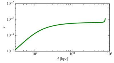
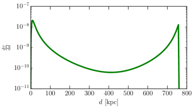
In Fig. 6, we show the optical depth of PBH microlensing for a single star in M31, calculated using the above equation. Here we have assumed that all the DM in the halo regions of MW and M31 is composed of PBHs, i.e., $\Omega_{\rm PBH}/\Omega_{\rm DM}=1$. The optical depth for microlensing, $\tau\sim 10^{-6}$, is larger compared to that to LMC or a star cluster in MW ($\tau\sim 10^{-7}$) by an order of magnitude, due to the enormous volume and large mass content between the Earth and M31. The PBHs in each of the MW and M31 halos result in a roughly equal contribution to the optical depth to an M31 star. Although there is an uncertainty in the DM density in the inner region of MW or M31 (at radii $\lower 2.15277pt\hbox{$\;\buildrel<\over{\sim}\;$}10$ kpc) due to poorly-understood baryonic effects, the contribution is not large.

Figure 7: A schematic illustration of configurations of a lensing PBH and a source star in M31 in the lens plane, following Fig. 4 of Ref. [13]. The orbit of a lensing PBH, around a source star in M31 (placed at the origin in this figure), is parameterized as in the figure, which is used to derive the microlensing event rate (see text for details).

Next we estimate the rate for microlensing events with a given timescale for its light curve. First we model the velocity distribution of DM in the halo regions. We simply assume an isotropic Maxwellian velocity distribution for DM particles (e.g., [4]):

$$f(\mathbf{v};r)\mathrm{d}^{3}\mathbf{v}=\frac{1}{\pi^{3/2}v_{\rm c}(r)^{3}}\exp\left[-\frac{|\mathbf{v}|^{2}}{v_{\rm c}(r)^{2}}\right]\mathrm{d}^{3}\mathbf{v}$$ (12)

where $V_{\rm halo}(r)$ is the velocity dispersion at radius $r$ from the MW or M31 center. For $V_{\rm halo}(r)$, we assume that it is given as

$$v_{\rm c}(r)=\sqrt{\frac{GM_{\rm NFW}(<r)}{r}},$$ (13)

where $M_{\rm NFW}(<r)$ is the interior mass within radius $r$ from the halo center, defined as $M_{\rm NFW}(<r)=4\pi\rho_{s}r^{3}_{s}\left[\ln(1+c)-{c}/({1+c})\right]$, where $c=r/r_{s}$ for each of the MW and M31 halos.

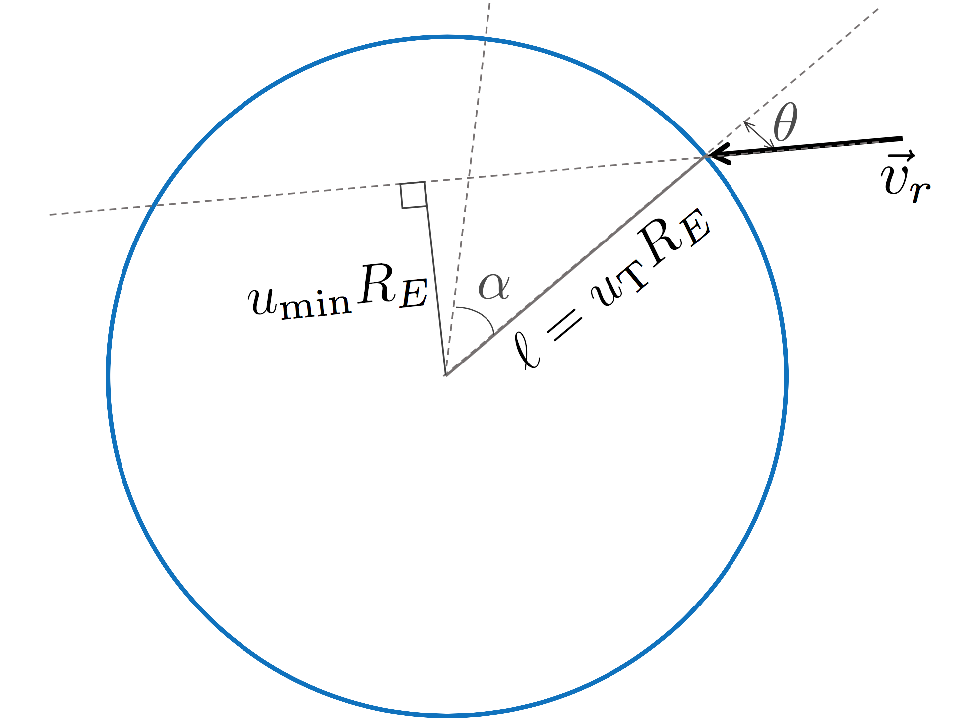
We start from the geometry and variables shown in Fig. 4 of Ref. [13] and their Eq. (10) (see Fig. 7), which gives the rate $\mathrm{d}\Gamma$ of PBHs entering a volume element along the line-of-sight where they can cause microlensing for a single star in M31:

$${\rm d}\Gamma=\frac{\Omega_{\rm PBH}}{\Omega_{\rm DM}}\frac{\rho_{\rm DM}(d)}{M_{\rm PBH}}\frac{u_{\rm T}R_{\rm E}}{\pi v_{\rm c}^{2}}\exp\left[-\frac{v_{\rm r}^{2}}{v_{\rm c}^{2}}\right]\,v_{\rm r}^{2}\cos\theta\,{\rm d}v_{\rm r}\,{\rm d}\theta\,{\rm d}d\,{\rm d}\alpha.$$ (14)

Here $n_{\rm PBH}(d)$ is the number density of PBHs at the distance $d$ from the Earth, $v_{\rm r}$ is the velocity of the PBH in the lens plane, $\theta$ is the angle at which the PBH enters the volume element, and $\alpha$ is an angle with respect to an arbitrary direction in the lens plane, as shown in Fig. 7. Microlensing events are identified if they have a given threshold magnification $A_{\rm T}$ at peak. This threshold magnification defines a threshold impact parameter with respect to the Einstein radius of a PBH, $u_{\rm T}=R_{\rm T}/R_{\rm E}$. Compared to Ref. [13], we have further ignored motions of source stars for simplicity, i.e. $v_{\rm t}=0$. The parameters vary in the range of $\theta\in[-\pi/2,\pi/2]$, $\alpha\in[0,2\pi]$, $v_{\rm r}=[0,\infty)$.

The timescale for the microlensing event described by the above geometry is given by $\hat{t}=2R_{\rm E}\cos\theta~{}u_{\rm T}/v_{\rm r}$. Thus the differential rate of microlensing events, occurring per unit timescale $\hat{t}$, is given by

$$\frac{{\rm d}\Gamma}{{\rm d}\hat{t}} = \frac{\Omega_{\rm PBH}}{\Omega_{\rm DM}}\int_{0}^{d_{\rm s}}\!\!{\rm d}d\int_{0}^{\infty}\!\!{\rm d}v_{\rm r}\,\int_{-\pi/2}^{\pi/2}\!\!{\rm d}\theta\int_{0}^{2\pi}\!\!{\rm d}\alpha\,\frac{\rho_{\rm DM}(d)}{M_{\rm PBH}}$$ (15)

$$\times\frac{u_{\rm T}R_{\rm E}}{\pi v_{\rm c}^{2}}\exp\left[-\frac{v_{\rm r}^{2}}{v_{\rm c}^{2}}\right]\,v_{\rm r}^{2}\cos\theta~{}\,\delta_{\rm D}\!\left(\hat{t}-\frac{2R_{\rm E}u_{\rm T}\cos\theta}{v_{\rm r}}\right).\hskip 10.00002pt$$

Using the Dirac-delta function identity,

$$\delta_{\rm D}\left(\hat{t}-\frac{2R_{\rm E}u_{\rm T}\cos\theta}{v_{\rm r}}\right)=\delta_{\rm D}\left(v_{\rm r}-\frac{2R_{\rm E}u_{\rm T}\cos\theta}{\hat{t}}\right)\frac{v_{\rm r}^{2}}{2R_{\rm E}u_{\rm T}\cos\theta},$$ (16)

and integrating over $\alpha$ and $v_{\rm r}$, we obtain

$$\frac{{\rm d}\Gamma}{{\rm d}\hat{t}}=\frac{\Omega_{\rm PBH}}{\Omega_{\rm DM}}\int_{0}^{d_{\rm s}}\!\!{\rm d}d\int_{-\pi/2}^{\pi/2}\!\!{\rm d}\theta\,\frac{\rho_{\rm DM}(d)}{M_{\rm PBH}v_{\rm c}^{2}}v_{\rm r}^{4}\,\exp\left[-\frac{v_{\rm r}^{2}}{v_{\rm c}^{2}}\right]\,,$$ (17)

with $v_{\rm r}=2R_{\rm E}u_{\rm T}\cos\theta/\hat{t}$. One can rewrite this equation by changing variable $\theta$ to the minimum impact $u_{\rm min}=u_{\rm T}\sin\theta$, such that, $\mathrm{d}\theta=\mathrm{d}u_{\rm min}/\sqrt{u_{\rm T}^{2}-u_{\rm min}^{2}}$. This results in

$$\frac{{\rm d}\Gamma}{{\rm d}\hat{t}}=2\frac{\Omega_{\rm PBH}}{\Omega_{\rm DM}}\int_{0}^{d_{\rm s}}\!\!{\rm d}d\int_{0}^{u_{T}}\!\!\frac{{\rm d}u_{\rm min}}{\sqrt{u_{\rm T}^{2}-u_{\rm min}^{2}}}\frac{\rho_{\rm DM}(d)}{M_{\rm PBH}v_{\rm c}^{2}}v_{\rm r}^{4}\exp\left[-\frac{v_{\rm r}^{2}}{v_{\rm c}^{2}}\right]\,,$$ (18)

where $v_{\rm r}=2R_{E}\sqrt{u_{\rm T}^{2}-u_{\rm min}^{2}}/\hat{t}$. To compute the event rate due to PBHs in both the halo regions of MW and M31, we sum the contributions, $\mathrm{d}\Gamma=\mathrm{d}\Gamma_{\rm MW}+\mathrm{d}\Gamma_{\rm M31}$. As we described above, we can express the centric radius of each halo, $r$, entering into $v_{\rm c}(r)$, in terms of the distance to the lensing PBH, $d$; $r=r(d)$. Unless explicitly stated, we will employ $u_{\rm T}=1$ as our default choice. Note that the expected event number shown in Fig. 2, $\mathrm{d}N_{\rm event}/\mathrm{d}\ln t_{\rm FWHM}$, is related to $\mathrm{d}\Gamma$ via $\mathrm{d}\Gamma/\mathrm{d}\ln{t}_{\rm FWHM}=\mathrm{d}^{2}N_{\rm event}/\mathrm{d}\ln t_{\rm FWHM}\mathrm{d}t_{\rm obs}$, where $t_{\rm obs}$ is the unit observation time [hours]. Since our observation was done for 7 consecutive hours within one night under the similar weather conditions, $\mathrm{d}N_{\rm event}/\mathrm{d}\ln t_{\rm FWHM}=7\times\mathrm{d}\Gamma/\mathrm{d}\ln t_{\rm FWHM}$.

Figure 8: The differential event rate of PBH microlensing for a single M31 star (Eq. 18); the rate per unit observation time (hour), per a single source star in M31, and per unit timescale of the microlensing light curve (hour) for PBHs of a given mass scale. Here we assumed that all the DM in the MW and M31 halo regions is made of PBHs; $\Omega_{\rm PBH}/\Omega_{\rm DM}=1$. The $x$-axis is the full-width-half-maximum (FWHM) timescale of microlensing light curve. The lighter or heavier PBH has a shorter or longer timescale of microlensing light curve. The right panel shows the relative contribution to the microlensing event rate due to PBHs in either MW or M31 halo region, for the case of $M_{\rm PBH}=10^{-8}M_{\odot}$.

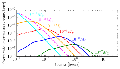
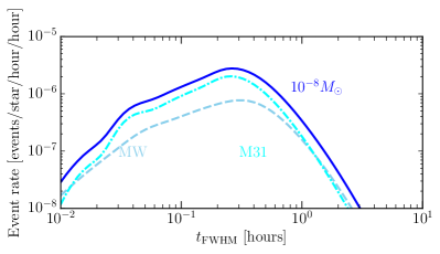
Fig. 8 shows the expected event rate for the PBH microlensing, computed using Eq. (18). Here we show the event rate as a function of the full-width-half-maximum (FWHM) timescale of the light curve, which matches our search of microlensing events from the real HSC data. If a PBH is in the mass range $M=[10^{-12},10^{-7}]M_{\odot}\simeq 2\times[10^{21},10^{26}]~{}{\rm g}$, it causes the microlensing event that has a typical timescale in the range of $[10^{-1},1]~{}$hour. The lighter or heavier PBHs tend to cause a shorter or longer timescale event. The event rate is quite high up to $10^{-4}$ for a microlensing timescale with $[0.1,1]~{}$hours. That is, if we take about 10 hours observation and observe $10^{8}$ stars at once for each exposure, we expect many events up to $10^{4}$ events (because $10^{-4}\times 10~{}[{\rm hour}]\times 0.1~{}[{\rm hour}]\simeq 10^{4}$), assuming that such PBHs constitute a majority of DM in the intervening space bridging MW and M31. The right figure shows that the PBHs in the M31 halo region give a slightly larger contribution to the event rate, because we assumed a larger halo mass for M31 than that of MW. Thus the high-cadence HSC observation of M31 is suitable for searching for microlensing events of PBHs.

1.3 Light curve characterization in pixel lensing regime

As we described above, the timescale for the PBH and M31 star microlensing system is typically several tens of minutes for a PBH with $10^{-8}M_{\odot}$. However, there is an observational challenge. Since the M31 region is such a dense star field, fluxes from multiple stars are overlapped in each CCD pixel ($0.168^{\prime\prime}$ pixel scale for HSC/Subaru). In other words individual stars are not resolved even with the Subaru angular resolution (about $0.6^{\prime\prime}$ for the seeing size). Hence we cannot identify which individual star in M31 is strongly lensed by a PBH, even if it occurs. Such a microlensing of unresolved stars falls in the “pixel microlensing” regime [25] (also see [26] for a review).

To identify microlensing events in the pixel microlensing regime requires elaborate data reduction techniques. In this paper, we use the image subtraction or image difference technique first described in Ref. [28]. The image difference technique allows us to search for variable objects including candidate stars that undergo microlensing by PBHs. In brief, starting with the time sequenced $N_{\rm exp}$ images of M31, the analysis proceeds as follows. (i) We generate a reference image by co-adding some of the best-seeing images in order to gain a higher signal-to-noise. Next we subtract this reference image from each of the $N_{\rm exp}$ images after carefully matching their point spread functions (PSFs) as described in Ref. [28]. (ii) We search for candidate variable objects that show up in the difference image. In reality, if the image subtraction is imperfect, the difference image would contain many artifacts, as we will discuss further. (iii) Once secure variable objects are detected, we determine the position (RA and dec) of each variable object in the difference image. We perform PSF photometry for each variable candidate using the PSF center to be at the position of the candidate in the difference image. By repeating the PSF photometry in each difference image of the $N_{\rm exp}$ images, we can measure the light curve of the candidate as a function of the observation time.

The light curve of a microlensing event obtained using the PSF flux in the difference image at time $t$, obtained as described above, can be expressed as

$$\Delta F(t)=F_{0}\left[A(t)-A(t_{\rm ref})\right],$$ (19)

where $\Delta F(t)$ is the differential flux of the star at time $t$ relative to the reference image, $F_{0}$ is the intrinsic flux, $A(t)$ is the lensing magnification at $t$ and $A(t_{\rm ref})$ is the magnification at the time of the reference image, $t_{\rm ref}$. In the above equation, $\Delta F(t)$ is a direct observable, and others ($F_{0},A(t),A(t_{\rm ref})$) are parameters that have to be modeled.

As can be seen from Eq. (2), the light curve for the microlensing of a point source by a point mass can be characterized by two parameters. The first parameter is the maximum amplification $A_{0}=A(u_{\rm min})$ when the lensing PBH is closest to a source star on the sky, where $u_{\rm min}$ is the impact parameter relative to the Einstein radius $R_{E}$ ($u_{\rm min}$ is dimension-less). The second one is the timescale of the light curve, which depends on the Einstein radius as well as the transverse velocity of the PBH moving across the sky. For the timescale parameter we use the FWHM timescale of the microlensing light curve, $t_{\rm FWHM}$, instead of $t_{E}$, defined as

$$A\left(\frac{t_{\rm FWHM}}{2}\right)-1\equiv\frac{A_{0}-1}{2}.$$ (20)

Thus the light curve of microlensing can be fully modeled by the three parameters, $F_{0}$, $u_{\rm min}$ and $t_{\rm FWHM}$. In the following we will use the three parameters when performing a fitting of the microlensing model to the observed light curve of microlensing candidate in the image difference. Note that the use of $t_{\rm FWHM}$, instead of $t_{E}$, gives slightly less degenerate constraints on the parameters [6].

2 Data Analysis and Object Selection

2.1 Observations

Figure 9: The background image of M31 shows configuration of 104 CCD chips of the Subaru/HSC camera. The white-color grids are the HSC “patch” regions. The patches labeled as “patch-D1”, “patch-D2” and “patch-H” are taken from representative regions of the disk region closer to the central bulge, the outer disk region and the halo region, respectively, which are often used to show example results of our data processing in the main text. The dark-blue regions are the patches we exclude from our data analysis due to too dense star fields, where fluxes from stars are saturated and the data are not properly analyzed.

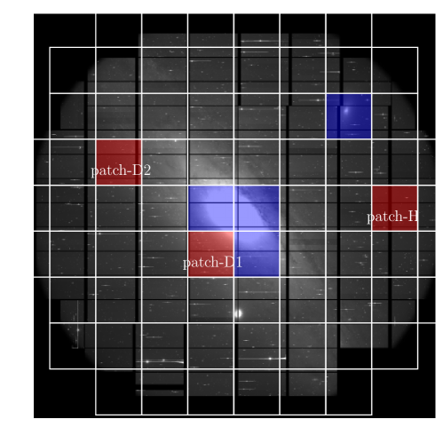
The HSC camera has 104 science detectors with a pixel scale of $0.168^{\prime\prime}$ [19]. The 1.5 degree diameter FoV of HSC enables us to cover the entire region of M31, from the inner bulge to the outer disk and halo regions with a single pointing. The pointing is centered at the coordinates of the M31 central region: (RA, dec) = (00h 42m 44.420s,+41d 16m 10.1s). We do not perform any dithering between different exposures in order to compare stars in the same CCD chip, which makes the image difference somewhat easier. However, in reality the HSC/Subaru system has some subtle inaccuracies in its auto-guidance and/or pointing system. This results in variations in the pointings of different exposures, typical variations range from a few to a few tens of pixels.

Fig. 9 shows the configuration of the 104 CCD chips relative to the image of M31 on the sky. The white-color boxes denote locations of HSC “patches”, which are convenient tessellations of the HSC FoV. The image subtraction and the search of microlensing events will be done on a patch-by-patch basis. The patches labeled “patch-D1”, “patch-D2” and “patch-H” denote the regions that represent inner and outer disk regions (-D1 and -D2) and a halo (-H) region, respectively. These representative regions will be used to show how the results vary in the different regions.

Figure 10: The PSF FWHM (seeing size) of each exposure (90 sec exposure each) as a function of time $t~{}$[sec] from the start of our observation. We took the images of M31 region every 2 min (90 sec exposure plus about 35 sec for readout), and have 188 exposures in total. The red points show the images of 10 best-seeing epochs ($\sim 0.45^{\prime\prime}$) from which the reference image, used for the image difference, was constructed.

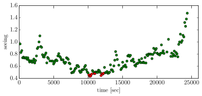
Our observation was conducted on November 23, 2014 which was a dark night, a day after the new moon. In total, we acquired 194 exposures of M31 with the HSC $r$-band filter, for the period of about 7 hours, until the elevation of M31 fell below about $30$ degrees. We carried out the observation with a cadence of 2 minutes, which allows us to densely sample the light curve for each variable object. The total exposure time was 90 seconds on source and about 35 seconds were spent for readout on average. The weather was excellent for most of our observation as can be seen from Fig. 10, which shows how the seeing FWHM changed with time from the start of our observation. The seeing size was better than $0.7^{\prime\prime}$ for most of the observation period, with a best seeing FWHM of about $0.4^{\prime\prime}$ at $t\sim 10,000~{}$sec (2.8 hours). However, the seeing got worse than $1^{\prime\prime}$ towards the end of our observation. We exclude 6 exposures which had seeing FWHM worse than $1.2^{\prime\prime}$ and use the remaining 188 exposures for our science analysis.

We also use the $g$- and $r$-band data, which were taken during the commissioning run on June 16 and 17 in 2013, respectively, in order to obtain color information of stars as well as to test a variability of candidates at different epochs. The $g$-band data consist of $5\times 120~{}{\rm sec}$ exposures and $5\times 30~{}{\rm sec}$ exposures in total, while the $r$-band data consists of $10\times 120~{}{\rm sec}$ exposures.

2.2 Data reduction and Sample selection

2.2.1 Standard data processing

We performed basic standard data reduction with the dedicated software package for HSC, hscPipe (version 3.8.6; also see Bosch et al. [29]), which is being developed based on the Large Synoptic Survey Telescope software package [7, 8, 9] . This pipeline performs a number of common tasks such as bias subtraction, flat fielding with dome flats, coadding, astrometric and photometric calibrations, as well as source detection and measurements.

After these basic data processing steps, we subtract the background contamination from light diffusion of atmosphere and/or unknown scattered light. However the background subtraction is quite challenging for the M31 region, because there is no blank region and every CCD chip is to some extent contaminated by unresolved, diffuse stellar light. To tackle this problem, we first divide each CCD chip into different meshes (the default subdivision is done into 64 meshes in each CCD chip). We then employ a higher-order polynomial fitting to estimate a smooth background over different meshes. We employed a 10-th order polynomial fitting for the CCD chips around the bulge region, which are particularly dense star regions. For other CCD chips, we use a 6-th order polynomial fitting scheme. However, we found residual systematic effects in the background subtraction, so we will further use additional correction for photometry of the difference image, as we will discuss later.

For our study, accurate PSF measurements and accurate astrometric solutions are crucial, because those allow for an accurate subtraction of different images. The pipeline first identifies brightest star objects ($S/N\lower 2.15277pt\hbox{$\;\buildrel>\over{\sim}\;$}50$) to characterize the PSF and do an initial astrometric and photometric calibration. From this initial bright object catalog, we select star candidates in the size and magnitude plane for PSF estimation (see Ref. [29] for details). The selected stars are fed into the PSFEx package [10] to determine the PSF as a function of positions in each CCD chip. The functional form of the PSF model is the native pixel basis and we use a second-order polynomial per CCD chip for the spatial interpolation. For the determination of the astrometry, we used a 30 sec calibration image that we took at the beginning of our observation, where bright stars are less saturated. We obtain an astrometry solution after every 11 images, 30 sec calibration frame plus 10 time-consecutive science exposures, by matching the catalog of stars to the Pan-STARRS1 system [11, 12, 13]. The HSC pipeline provides us with a useful feature, the so-called “hscMap”, which defines a conversion of the celestial sphere to the flat coordinate system, “hscMap coordinate”, based on a tessellation of the sky. In Fig. 9 the white-color regions denote the hscMap “patch” regions. We perform image difference separately on each patch. Due to too many saturated stars in the bulge region and M101, we exclude the patches, marked by dark blue color, from the following analysis.

2.2.2 Image subtraction and object detection

In order to find variable objects, we employ the difference image technique developed in Alard & Lupton (1998; [28]) (also see Ref. [14]), which is integrated into the HSC pipeline. To do this, we first generated the “reference” image by co-adding 10 best-seeing images among the 188 exposure images, where the 10 images are not time-consecutive (most of the 10 images are from images around about 3 hours from the beginning of the observation, as shown in Fig. 10). We use the mean of the 10 images as the observation time of the reference image, $t_{\rm ref}$, which is needed to model the microlensing light curve (Eq. 19).

In order to make a master catalog of variable object candidates, we constructed 63 target images by co-adding 3 time-consecutive images from the original 188 exposure images. A typical limiting magnitude is about 26 mag (5$\sigma$ for point sources), and even better for images where seeing is good (see below). When subtracting the reference image from each target image, the Alard & Lupton algorithm uses a space-varying convolution kernel to match the PSFs of two images. The optimal convolution kernel is derived by minimizing the difference between convolved PSFs of two images. A variable object, which has a flux change between the two images, shows up in the difference image.

Fig. 3 shows an example of the image subtraction performed by the pipeline. Even for a dense star region in M31, the pipeline properly subtracts the reference from the target image, by matching the PSFs and astrometry. A point source which undergoes a change in its flux shows up in the difference image, as seen in the right panel. In this case, the candidate appears as a black-color point source meaning a negative flux, because it has a fainter flux in the target image than in the reference image.

We detect objects in the difference image each of which is defined from a local minimum or maximum in the difference image, where we used $5\sigma$ for the PSF magnitude as detection threshold. The pipeline also measures the center of each object and the size and ellipticity from the second moments. In this process we discarded objects that have ill-defined center, a saturated pixel(s) in the difference and/or original image or if the objects are placed at a position within 50 pixels from the CCD edge.

2.2.3 PSF photometry and master catalog of variable star candidates

For each variable star candidate, we obtain PSF photometry in the difference image to quantify the change of flux. We allow negative PSF fluxes for candidates that have fainter flux in the target image than in the reference image. Since the photon counts in each CCD pixel is generally contaminated by multiple stars in most of the M31 regions, we often find a residual coherent background (large-scale modulated background) in each difference image, due to imperfect background subtraction in the original image. To avoid contamination from such a residual background, we first measure the spatially constant background from the median of counts in $41\times 41$ pixels around each object in the postage-stamp image, and then subtract this background from the image. Then we perform the PSF-photometry counts in ADU units taking the PSF center to be at the candidate center. Hereafter we sometimes refer to PSF magnitude in the difference image as “PSF counts”. The pipeline also estimates noise in each pixel assuming the background limit (Poisson noise), and gives an estimation of the noise for the PSF photometry (see Eqs. 14 and 15 in Ref. [15] for the similar definition). However, the noise estimation involves a non-trivial propagation of Poisson noise in the image difference procedures, so we will use another estimate for the PSF photometry error in each patch, as described below.

In the following we focus on the PSF photometry counts in ADU units in the difference image, rather than the magnitude, because it is a direct observable in our analysis. However, we will also need to infer the magnitude of each candidate; for example, to estimate the luminosity function of source stars in each magnitude bin or to plot the light curve of variable star candidates in units of the magnitude. In this case we estimate the magnitude of an object in the $i$-th target image, $m_{i}$, based on

$$m_{i}=-2.5\log\left(\frac{C_{{\rm diff},i}+C_{\rm ref}}{F_{0,i}}\right),$$ (21)

where $C_{\rm diff},i$ is the PSF flux for the object in the difference image of the $i$-th target image, $C_{\rm ref}$ is the PSF flux of the reference image at the object position, and $F_{0,i}$ is the zero-point flux in the $i$-th image. Note that the counts of the reference image $C_{\rm ref}$ can be contaminated by fluxes from neighboring stars, so the above magnitude might not be accurate.

Figure 11: Examples of detected objects in the difference image, which pass or do not pass the selection criteria to define a master catalog of variable star candidates (see text for details). Each panel shows 4 postage-stamp images: the leftmost image is the reference image (the coadded image of 10 best-seeing exposures), the 2nd left is the target image (the coadded image of 3 time-consecutive exposures), the 3rd image is the difference image between the reference and target images, and the rightmost image is the residual image after subtracting the best-fit PSF image from the difference image at the object position. The two objects in top raw are successful candidates that passed all the selection criteria: the left-panel object has a brighter flux in the target image than in the reference image, while the right-panel object has a fainter flux (therefore appear as a black-color image with negative flux). The lower-row objects are removed from the catalog after the selection criteria. The objects in the middle row are excluded because the object is either smaller or larger than the PSF size. The left object in the bottom row is excluded because it has a too large ellipticity than PSF. The right object is excluded because of too large residual image.

From the initial catalog constructed from the $5\sigma$ candidates from the 63 coadded images, we prune it down to a master catalog of “secure” variable star candidates by applying the following criteria:

• PSF magnitude threshold – A candidate should have a PSF magnitude, with a detection significance of $5\sigma$ or higher (including a negative flux), in any of the 63 difference images.

• Minimum size – The size of the candidate should be greater than 0.75 times the PSF size of each difference image.

• Maximum size – The size of the candidate should be smaller than 1.25 times the PSF size.

• Roundness – The candidate should have a round shape. We require our candidates to have an axis ratio greater than 0.75, as the PSF does not show extreme axis ratios.

• PSF shape – We impose that the shape of an object should be consistent with the PSF shape. The residual image, obtained by subtracting a scaled PSF model from the candidate image in the difference image, should be within $3\sigma$ for the cumulative deviation over pixels inside the PSF aperture.

Fig. 11 shows examples of objects that pass or fail the above criteria. Note that the above conditions are broad enough in order for us not to miss a real candidate of microlensing if it exists. We make a master catalog of variable star candidates from objects that pass all the above conditions as well as are detected in the image difference at least twice in the 63 difference images at the same position within 2 pixels. These criteria result in 15,571 candidates of variable objects, which is our master catalog of variable star candidates.

2.2.4 Light curve measurement

Figure 12: Examples of light curves for real variable stars identified in our method. The green-circle data points show the light curve sampled by our original data of 2 min sampling rate, while the red-triangle points are the light curve measured from the coadded data of 3 time-consecutive exposures (therefore 6 min cadence) (see text for details). Upper left: candidate stellar flare. When converting the magnitude from the counts in the difference image at each observation time, we used Eq. (21). Note that the estimated magnitude might be contaminated by fluxes of neighboring stars in the reference image. Upper right: candidate contact binary stars. Lower left: the eclipse binary system, which is probably a system of white dwarf and brown dwarf, because one star (white dwarf) has a total eclipse over about 10 min duration, and then the eclipse has about 3 hours period. Lower right: candidate variable star, which has a longer period than our observation duration (7 hours).

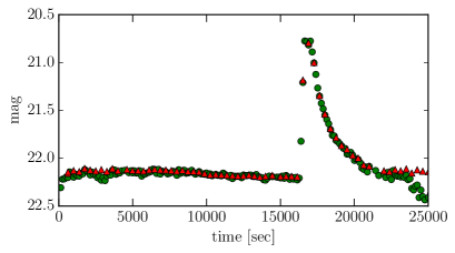
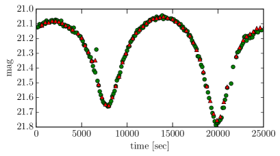
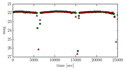
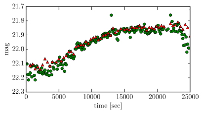
Once each candidate is identified, we measure the PSF counts in each of the 63 difference images. This allows us to measure the light curve with a 6 min resolution, as a function of time from the beginning to the end of our 7 hour long observations. In order to restore the highest time resolution of our data, we then used each of 188 exposures and measured the PSF counts in each of the 188 difference image that was made by subtracting the reference image (the coadded image of 10 best-seeing exposures) from every single exposure. Here we used the same position of candidate as used in the 63 images. In this way we measure the light curve of the object with 2 min time resolution.

Fig. 12 shows the light curves for examples of real variable stars. Note that we converted the PSF counts of each candidate in the difference image to the magnitude based on Eq. (21). However, the magnitude might be contaminated by fluxes from blended stars surrounding the candidate star. The figure demonstrates our ability to properly sample the light curves with high time resolution. Thus the difference image technique works well and can identify variable star candidates as well as measure their light curves.

Figure 13: Distribution of secure variable star candidates, detected from our analysis using the image difference technique. The different symbols denote different types of candidates classified based on the shapes of their light curves. Here we exclude other non-secure candidates that are CCD artifacts and impostors near to the CCD edge or bright stars. The left panel shows the distribution for the candidates with magnitudes $m_{r}\leq 24~{}$mag, while the right panel shows the candidates at $m_{r}\leq 25~{}$mag. The number of candidates are 1,334 and 2,740, respectively.

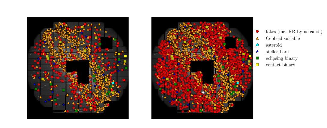
Fig. 13 shows the distribution of secure variable star candidates detected in our analysis over the HSC field-of-view, for candidates with magnitudes $m_{r}\leq 24$  and 25 mag in the left and right panel, respectively. To estimate the magnitude of each candidate, we used the PSF magnitude of the candidate in the reference image. Based on the shape of the light curve for each candidate, we visually classified the candidates in different types of variable stars; i) stellar flares, ii) eclipsing or contact binary systems, iii) asteroids (moving object), iv) Cepheid variables if the candidates appear to have a longer period than our observation duration (7 hours), and v) “impostors”. Here impostors are those candidates which show time variability only when the seeing conditions are as good as $\lower 2.15277pt\hbox{$\;\buildrel<\over{\sim}\;$}0.6^{\prime\prime}$. Since such good-seeing data is deeper as found from Figs. 10 and 14, we seem to find RR-Lyrae type variables whose apparent magnitudes would be around $r\sim 25~{}$mag. When the seeing gets worse, these stars cannot be reliably seen in the difference image. Since RR-Lyrae stars should exist in the M31 region, we think the “impostor” stars are good candidates for RR-Lyrae stars. The figure shows that our analysis successfully enables to find variable stars across the disk and halo regions. The total number of candidates are 1,334 and 2,740 for $m_{r}\leq 24~{}$ and 25 mag, respectively.

3 Statistics and Selection Criteria

Given the catalog of variable star candidates each of which has its measured light curve, we now search for secure candidates of PBH microlensing. In this section we describe our selection criteria to discriminate the microlensing event from other variables.

3.1 Photometric errors of the light curve measurement

Figure 14: The photometric error used for the light curve measurement in the difference image; we randomly select 1,000 points in the difference image of a given patch (here shown for the patch-D2 in Fig. 9), measure the PSF photometry at each random point, and then estimate the variance of the PSF photometries (see text for details). The square symbols show the 3- or 5-sigma photometric errors estimated from the variance when using the difference images constructed from the coadded images of 3 exposures, as a function of observation time. The circle symbols, connected by the line, are the results for each exposure. Although we use the photometric error in the ADU counts for a fitting of the microlensing model to the light curve, we here convert the counts to the magnitude for illustrative convenience.

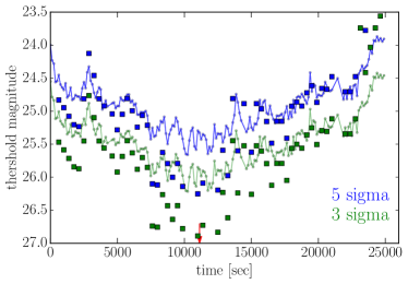
Our primary tool to search for variable objects in the dense star regions of M31 is the use of the image difference technique, as we have shown. To robustly search for secure candidates of PBH microlensing that have the expected light curve shapes, it is crucial to properly estimate the photometry error in the light curve measurement. However, accurate photometry for dense star regions in M31 is challenging. To overcome this difficulty, we use the following approach to obtain a conservative estimate of the error. The pipeline performs image subtraction on each patch basis (as denoted by white-color square regions in Fig. 9). For a given difference image, we randomly select 1,000 points in each patch region, and then perform PSF photometry at each random point in the same manner as that for the variable star candidates. In selecting random points, we avoided regions corresponding to bad CCD pixels or near the CCD chip edges. We then estimate the variance from those 1,000 PSF magnitudes, repeat the variance estimation in the difference image for every observation time, and use the variance as a $1\sigma$ photometry error in the light curve measurement at the observation time. The photometric error estimated in this way would include a contamination from various effects such as a large-scale residual background due to an imperfect background subtraction. We find that the photometric error is larger than the error estimated from the pipeline at the candidate position, which is locally estimated by propagating the Poisson noise of the counts through the image subtraction processes.

Fig. 14 shows the photometric error on the light curve measurement in the difference image, estimated based on the above method. The shape of the photometric error appears to correlate with the seeing conditions in Fig. 10. The figure shows that most of our data reaches a depth of 26 mag or so thanks to the 8.2m large aperture of Subaru.

3.2 Microlensing model fit to the light curve data

Table 1: Definitions of Statistics

Statistic	Definition
$\Delta C(t_{i})$	PSF-photometry counts of a candidate in the $i$-th difference image at the observation time $t_{i}$;
	the time sequence of $\Delta C(t_{i})$ forms the light curve of each candidate (188 data points,
	sampled by every 2 min).
$\Delta C_{{\rm coadd}}(t_{i})$	PSF-photometry counts of a candidate in the $i$-th difference image of 3 coadded images at $t_{i}$
	(63 data points, sampled by every 6 min)
$\sigma_{i}$	$1\sigma$ error of PSF-photometry in the $i$-th difference image (see text for details)
$\sigma_{{\rm coadd},i}$	$1\sigma$ error in the $i$-th difference image of 3 coadded images at $t_{i}$
bump	sequence of 3 or more time-consecutive data points with $\Delta C_{i}\geq 5\sigma_{i}$ in the light curve
bumplen	length (number) of time-consecutive data points with $\Delta C_{i}\geq 5\sigma_{i}$
mlchi2_dof	$\chi^{2}$ of the light curve fit to microlensing model divided by the degrees of freedom
mlchi2in_dof	$\chi^{2}$ of the microlensing fit for data points with $t_{i}$ satisfying $t_{0}-t_{\rm FWHM}^{\rm obs}\leq t_{i}\leq t_{0}+t^{\rm obs}_{\rm FWHM}$
asymmetry $a_{\rm asy}$	$(1/N_{\rm asy})\left.\sum_{t_{i}}\left[\Delta C(t_{0}-\Delta t_{i})-\Delta C(t_{0}+\Delta t_{i})\right]\right/[\overline{\Delta C}-\Delta C_{\rm min}]$ (see text for details)
seeing_corr	correlation between the light curve shape and the seeing variation (see text for details)

Table 2: Selection Criteria

Selection Criterion	Purpose	No. of remained candidates
$\Delta C_{{\rm coadd},i}\geq 5\sigma_{{\rm coadd},i}$	initial definition of candidates	15,571
bumplen$\geq 3$	select candidates with a significant peak(s) in the light curve	11,703
mlchi2dof$<3.5$	select candidates whose light curve is reasonably well fit	227
	by the microlensing
$a_{\rm asy}<0.17$	remove candidates that have an asymmetric light curve such	146
	as star flares
significant peak	select candidates that show a clear peak in its light curve	66
	(see text for details)
visual inspection	visually check each candidate (its light curve and images)	1
seeing_corr	remove candidates whose light curve is correlated with time	1
	variation of seeing

Figure 15: Example of the light curves of candidates that are rejected by our selection criteria for a microlensing event. The red points in each panel shows the PSF photometry at each observation time and consist of 188 data points to form the light curve sampled by every 2 min in the difference images. The errorbar around each data point is the photometry error that is locally estimated by propagating the Poisson noise of counts through the difference image processes at the candidate position. The range bracketed by the two data points around zero counts is the $\pm 1\sigma$ photometry error that is estimated from the PSF photometries of 1,000 random points as shown Fig. 14. The blue data points are the light curve for the best-fit microlensing model. The upper-left panel shows an example of the candidates that is rejected due to a bad $\chi^{2}_{\rm min}$ for the fitting to the microlensing light curve. The upper-right panel shows an example of the candidates that is rejected by the asymmetric shape of the light curve around the peak. The lower two panels show examples of the candidates that do not show a prominent peak feature as expected for a microlensing event.

Figure 16: The upper panel shows an example of light curves for impostors that are caused by a spike-like image around a bright star. The light curve appears to look like a microlensing event, but it is found to be near a bright star. The lower panel shows the light curve for an asteroid that also shows a microlensing-like light curve. If the PSF photometry is made at the fixed position (the center in the lower-right image), the measured light curve looks like a microlensing event. The red points in the image denotes the asteroid trajectory. From our analysis of M31 observation, we identified one asteroid.

Here we describe our selection procedure for PBH microlensing events from the candidates. The unique part of our study is the the high cadence for the light curve of each candidate, sampled by every 2 min over about 7 hours. However the monitoring of each light curve is limited by a duration of 7 hours. If a microlensing event has a longer time duration than $7~{}$hours, we can not identify such a candidate. We use the statistics in Table 1 to quantify the characteristics of each light curve. Our selection procedure for the candidates are summarized in Table 2. We will describe each of the selection steps in detail.

As we described, we start with the master catalog of variable star candidates, which contains 15,571 candidates, to search for microlensing events. Our level 1 requirement is that a candidate event should have a “bump” in its light curve, defined as 3 time-consecutive flux changes each of which has a signal-to-noise ratio greater than $5\sigma$ in the difference image; $\Delta C_{i}\geq 5\sigma_{i}$, where the subscript $i$ denotes the $i$-th difference image (at the observation time $t_{i}$). This criteria leaves us with $11,703$ candidates over all the patches.

Next we fit the observed light curves of each candidate with a model describing the expected microlensing light curve. As we described in Section 1.3, the light curve of a microlensing in the difference image is given as

$$\Delta C(t_{i})=C_{0}\left[A(t_{i})-A(t_{\rm ref})\right],$$ (22)

where $C_{0}$ is the PSF-photometry counts of an unlensed image in the difference image, corresponding to $F_{0}$ in Eq. (19), and $A(t_{i})$ and $A(t_{\rm ref})$ are lensing magnifications at the observation time $t_{i}$ and the time of the reference image $t_{\rm ref}$. As described in Section 1.3, the light curve in the difference image is characterized by 3 parameters: $(u_{\rm min},t_{\rm FWHM},C_{0})$, where $u_{\rm min}$ is the impact parameter of closest approach between PBH and a source star in units of the Einstein radius, and $t_{\rm FWHM}$ is the FWHM timescale of the light curve.

We identify the time of maximum magnification in the light curve and denote it by $t_{\rm 0}$. For the model fitting, we employ the following range for the model parameters:

• $0.01\leq u_{\rm min}<1$, which determines the maximum magnification, $A_{\rm max}\equiv A(u_{\rm min})$ (see Eq. 2). Thus we assume the range of maximum magnification to be $1.34\leq A_{\rm max}\lower 2.15277pt\hbox{$\;\buildrel<\over{\sim}\;$}100$.

• $0.01\leq t_{\rm FWHM}/[{\rm sec}]<25,000$. Here the lower limit is much shorter than the sampling rate of light curve (2 min), but we include such a short time-scale light curve for safety (see below). The upper limit corresponds to the longest duration of our observation ($\sim 7~{}$hours).

• Once the parameters, $u_{\rm min}$ and $t_{\rm FWHM}$, are specified, the intrinsic flux can be estimated as $C_{0}=\Delta C_{\rm max}^{\rm obs}/[A_{\rm max}-A(t_{\rm ref})]$, where $\Delta C_{\rm max}^{\rm obs}$ is the counts of the light curve peak in the difference image. In practice, the flux measurement is affected by measurement noise as well as the sampling resolution of light curve, so we allow the intrinsic flux to vary in the range of $0.5\times\Delta C_{\rm max}^{\rm obs}/(A_{\rm max}-1)\leq C_{0}\leq 1.5\times\Delta C_{\rm max}^{\rm obs}/(A_{\rm max}-1)$.

The above ranges of parameters are broad enough in order for us not to miss a real candidate of microlensing. For each candidate, we perform a standard $\chi^{2}$ fit by comparing the model microlensing light curve to the observed light curve:

$$\chi^{2}=\sum_{i=1}^{188}\frac{\left[\Delta C^{\rm obs}(t_{i})-\Delta C^{\rm model}(t_{i};C_{0},t_{\rm FWHM},u_{\rm min})\right]^{2}}{\sigma_{i}^{2}},$$ (23)

where $\Delta C^{\rm model}(t_{i})$ is the model light curve for microlensing, given by Eq. (22), and $\sigma_{i}$ is the rms noise of PSF photometry in the $i$-th difference image, estimated from the 1,000 random points as described above.

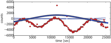
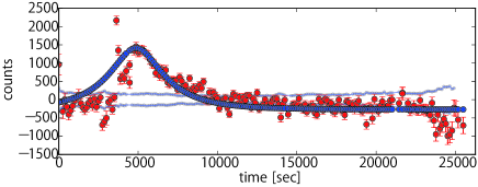
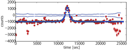
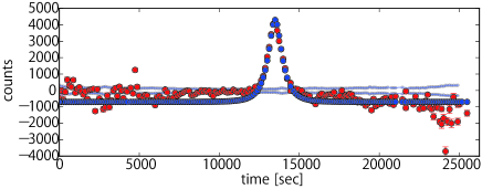
We compute the reduced $\chi^{2}$ by dividing the minimum $\chi^{2}$ by the degrees of freedom (188-3=185). We discard candidates that have ${\rm mlchi2\_dof}>3.5$. This criterion is reasonably conservative (the P-value is $\sim 10^{-5}$). We further impose the condition that the best-fit $t_{\rm FWHM}<14,400~{}$sec (4 hours), in order to remove candidates whose light curve has a longer time variation than what we can robustly determine. This selection removes most of Cepheid-type variables. This selection leaves 225 candidates. The upper-left panel of Fig. 15 shows an example of candidates that are removed by the condition ${\rm mlchi2\_dof}<3.5$ (i.e. ${\rm mlchi2\_dof}>3.5$ for this candidate). This is likely to be a binary star system.

Microlensing predicts a symmetric light curve with respect to the maximum-magnification time $t_{0}$ ($A_{\rm max}$); the light curve at $t_{i}=|t_{0}\pm\Delta t|$ should have a similar flux as the lensing PBH should have a nearly constant velocity within the Einstein radius. Following [18], we define a metric to quantify the asymmetric shape of the light curve,

$$a_{\rm asy}=\frac{1}{N_{\rm asy}}\sum_{t_{i}\in|t_{0}\pm t_{\rm FWHM}^{\rm obs}|}\frac{\left|\Delta C(t_{0}-\Delta t_{i})-\Delta C(t_{0}+\Delta t_{i})\right|}{\overline{\Delta C}-\Delta C_{\rm min}}.$$ (24)

Here $t_{\rm FWHM}^{\rm obs}$ is the timescale that the observed light curve declines to half of its maximum value. For this purpose, we take the longer of the timescales from either side of the two half-flux points from the maximum peak. If the expected half-flux data point is outside the observation window of light curve, we take the other side of the light curve to estimate $t_{\rm FWHM}^{\rm obs}$. The summation runs over the data points satisfying $t_{i}\leq|t_{0}\pm t_{\rm FWHM}^{\rm obs}|$, 2 times the FWHM timescale around the light curve peak. Note that, if the summation range is outside the observation window, we take the range $|t_{0}\pm(t_{0}-t_{\rm start})|$ or $|t_{0}\pm(t_{\rm end}-t_{0})|$, where $t_{\rm start}$ or $t_{\rm end}$ is the start or end time of the light curve. $N_{\rm asy}$ is the number of data points in the above summation, $\overline{\Delta C}$ is the average of the data points taken in the summation, and $\Delta C_{\rm min}$ is the minimum value of the counts.

By imposing the condition $a_{\rm asy}<0.17$, we eliminate candidates that have an asymmetric light curve, and we have confirmed that this condition eliminates most of the star flare events from the data base. This condition also eliminates some of the variable stars that are likely to be Cepheids. After this cut the number of candidates is reduced to $146$. The upper-right panel of Fig. 15 shows an example of the candidates that are removed by the condition $a_{\rm asy}<0.17$.

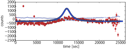
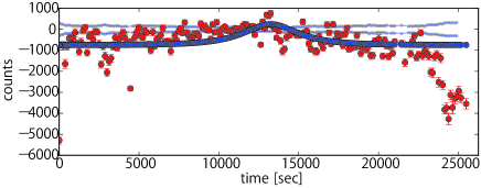
In addition we discard candidates, if the observed light curve does not have any significant peak; e.g., we discard candidates if ${\rm mlchi2in\_dof}>3.5$ (see Table 1 for the definition) or if the time of the light-curve peak is not well determined. The lower panels of Fig. 15 show two examples of such rejected candidates, which do not show a clear bump feature in the light curve as expected for microlensing. This selection cut still leaves us with 66 candidates.

Finally we perform a visual inspection of each of the remaining candidates. We found various impostors that are not removed by the above automated criteria. Most of the impostors are caused by an imperfect image subtraction; in most cases the difference image has significant residuals near the edges of CCD chips and around bright stars. In particular, bright stars cause a spiky residual image in the difference image, that results in impostors that have microlensing-like light curve if measured at a fixed position. We found 44 impostors caused by such spike-like images around bright stars. There are 20 impostors around the CCD edges. The upper panel of Fig. 16 shows an example of spike-like impostors. We were also able to identify 1 impostor caused by a moving object, an asteroid. If the light curve is measured at the fixed position which the asteroid is passing, it results in a light curve which mimics microlensing, as shown in the lower panel of Fig. 16.

Thus our visual inspection leads us to conclude that 65 events among 66 remaining candidates are impostors and we end up with one candidate event which passes all our cuts and visual checks. The candidate position is $({\rm RA},{\rm dec})=(00{\rm h}~{}45{\rm m}~{}33.413{\rm s},+41{\rm d}~{}07{\rm m}~{}53.03{\rm s})$.

Figure 17: One remaining candidate that passed all the selection criteria of microlensing event. The images in the upper plot show the postage-stamped images around the candidate as in Fig. 11: the reference image, the target image, the difference image and the residual image after subtracting the best-fit PSF image, respectively. The lower panel shows that the best-fit microlensing model gives a fairly good fitting to the measured light curve.

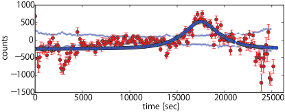
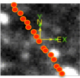
Fig. 17 shows the images and the light curve for this candidate of microlensing event. Although the light curve looks noisy, it is consistent with the microlensing prediction. The magnitude inferred from the reference image implies that the candidate has a magnitude of $r\sim 24.5~{}{\rm mag}$. The obvious question to consider is whether this candidate is real. Unfortunately, the candidate is placed outside the survey regions of the Panchromatic Hubble Andromeda Treasury (PHAT) catalog in [30] (also see [31]) , so the HST image is not available. It is unclear if there are any variable stars that could produce the observed light curve, with a single bump. To test the hypothesis that the candidate is a variable star, we looked into another $r$-band data that was taken in the commissioning run in 2013, totally different epoch from our observing night. However, the seeing condition of the $r$-band is not good (about $1.2^{\prime\prime}$), so it is difficult to conclude whether the star pops out of the noise in the difference images. Similarly we looked into the $g$-band images taken in the HSC commissioning run. However, due to the short duration of the data itself ($\sim 15~{}$min), it is difficult to judge whether this candidate has a time variability between the $g$ images. Hence we cannot draw any convincing conclusion on the nature of this candidate. In what follows, we derive an upper bound on the abundance of PBHs as a constituent of DM for both cases where we include or exclude this remaining candidate.

4 Results: Upper Bound on the Abundance of PBH Contribution to Dark Matter

In this section we describe how we use the results of our PBH microlensing search to derive an upper limit on the abundance of PBHs assuming PBHs consist of some fraction of DM in the MW and M31 halos. In order to do this, we need three ingredients – (1) the event rates of microlensing as we estimated in Section 1.2, (2) a detection efficiency for PBH microlensing events, which quantifies the likelihood of whether a microlensing event, even if it occurs during our observation duration, will pass all our selection cuts, and (3) the number of source stars in M31. In this section we describe how to estimate the latter two ingredients and then derive the upper bound result.

4.1 Efficiency calculation: Monte Carlo simulation

Figure 18: The detection efficiency estimated from light curve simulations taking into account the PSF photometry error in each of 188 target images we used for the analysis (see text for details). Here we generated Monte Carlo simulations of microlensing events randomly varying the three parameters: the impact parameter (or maximum lensing magnification), the FWHM timescale of microlensing light curve ($x$-axis), and the observation time of the microlensing magnification peak, for source stars of a fixed magnitude as indicated by legend. The detection efficiency for each source magnitude is estimated from 1,000 realizations.

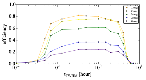
The detection efficiency of PBH microlensing events depends upon the unlensed flux of the star in M31, $F_{0}$, and quantifies the fraction of microlensing events with a given impact parameter ($u_{\rm min}$) and timescale ($t_{\rm FWHM}$) that can be detected given our selection cuts.

To estimate the efficiency we carry out simulations of microlensing light curves. We vary the model parameters to generate a large number of realizations of the simulated microlensing light curves. First we randomly select the time of maximum magnification ($t_{\rm max}$) from the observation window, the impact parameter $u_{\rm min}\in[0,1]$ and the FWHM timescale $t_{\rm FWHM}$ in the range of $0.01\leq t_{\rm FWHM}/[{\rm sec}]\leq 25,000~{}$ to simulate the input light curve in the difference image for a given intrinsic flux of a source star, $F_{0}$ (more precisely, the intrinsic counts $C_{0}$ in the difference image). Then, we add random Gaussian noise to the light curve at each of the observation epochs $t_{i}$, estimated from the $i$-th difference image in a given patch (Section 3.1). For each intrinsic flux, we generate 10,000 simulated light curves in each patch region.

For each simulated light curve, we applied all of our selection cuts (see Section 3 and Tables 1 and 2) to assess whether the simulated event passes all the criteria. Fig. 18 shows the estimated efficiency for a given intrinsic flux of a star as a function of the timescale ($t_{\rm FWHM}$) of the simulated light curve, in the patch-D2 of Fig. 9. A microlensing event for a bright star is easier to detect, if it occurs, because even a slight magnification is enough to identify it in the difference image. On the other hand, a fainter star needs more significant magnification to be detected. If the microlensing timescale is in the range of $4~{}{\rm min}\lower 2.15277pt\hbox{$\;\buildrel<\over{\sim}\;$}t_{\rm FWHM}\lower 2.15277pt\hbox{$\;\buildrel<\over{\sim}\;$}3~{}{\rm hours}$, the event can be detected by our observation (2 min sampling rate and 7 hours observation). We interpolated the results for different intrinsic fluxes to estimate the detection efficiency for an arbitrary intrinsic flux. We repeated the simulations using the photometry errors to estimate the efficiency for each patch.

Figure 19: A justification of the detection efficiency estimation, based on the different method using the fake image simulations. We injected fake microlensing star images in individual exposures of the real HSC data (patch-D2 in Fig. 9), re-ran the whole data processing, and assessed whether the fake images pass all the selection criteria for a microlensing event. The small circles show the results from light curve simulations (the same as shown in Fig. 18), and the large symbols show the results from the fake image simulations, for the intrinsic magnitudes of 22 and 24 mag, respectively.

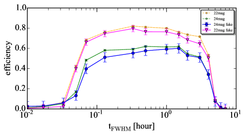
We also performed an independent estimation of the detection efficiency. We used fake image simulations where we injected fake microlensing star events into individual HSC images using the software GalSim in Refs. [16, 36], and then re-ran the whole data reduction procedure including image subtraction to measure the light curve. We then assessed whether the fake microlensing event can be detected by our selection criteria. Fig. 19 compares the detection efficiency estimated using the fake image simulations with the results of the simulated light curves (Fig. 18) in the patch-D2. The figure clearly shows that the two results fairly well agree with each other. The fake image simulations are computationally expensive. With the results in Fig. 19, we conclude that our estimation of the detection efficiency using the simulated light curves are fairly accurate.

4.2 Estimation of star counts in M31

Figure 20: An example image of the distribution of peaks (cross symbols) identified in a small region of the reference image (the coadded image of 10 best-seeing exposures), which has a size of about $38^{\prime\prime}\times 30^{\prime\prime}$ area and is taken from the patch-D2 region. We measure the PSF photometry of each peak, and then use the number of peaks as an estimation of the number of source stars in each magnitude bin.

Figure 21: The color scale denotes the total number of detected peaks in each patch region for the HSC data. Note that the black-color patches are excluded from our analysis due to too crowded regions. The number of the peaks in a disk region tends to be smaller than that in a outer, halo region, because stars in a disk region are more crowded and only relatively brighter stars or more prominent peaks are identified.

Figure 22: The peaks counts of HSC data in different regions of M31; two disk regions denoted as patch-D1 and patch-D2 and the halo region denoted as patch-H in Fig. 9. The HSC data can find a more number of fainter peaks in the halo regions because individual stars are more resolved and less crowded.

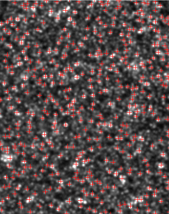
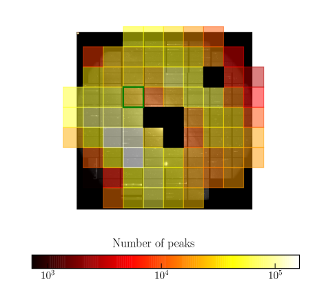
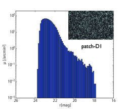
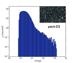
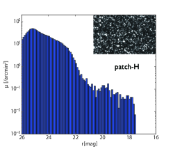
The expected number of microlensing events depends on the number of source stars in M31. However, since individual stars are not resolved in the M31 field, it is not straightforward to estimate the number of source stars from the HSC data. This is the largest uncertainty in our results, so we will discuss how the results change for different estimations of the source star counts. As a conservative estimate for the number of source stars, we use the number of “detected peaks” in the reference image of M31 data, which has the best image quality (coadding the 10 best-seeing exposures) and is used for the image subtraction. Fig. 20 shows the distribution of peaks identified from the reference image in an example region (with a size $226\times 178$ pixels corresponding to about $38^{\prime\prime}\times 30^{\prime\prime}$), taken from the patch-D2 region. The figure clearly shows that only relatively bright stars, or prominent peaks, are identified, but a number of faint stars or even bright stars in a crowded (or blended) region will be missed. Thus this estimate of the source star counts is extremely conservative. Nevertheless this is one of the most secure way to obtain source counts, so we will use these counts in each patch region.

The color scale in Fig. 21 shows the total number of peaks in each patch region. It can be seen that a relatively larger number of the peaks are identified in the outer halo region of M31, because each star can be resolved without confusion. On the other hand, there are less number of resolved peaks in the patches corresponding to the disk region due to crowding. The total number of peaks identified over all the patch regions is about 6.4 million. Fig. 22 shows the surface density of peaks identified in HSC in the disk and halo regions of M31 for the three patches marked in Fig. 9. To estimate the magnitudes for the surface density, we performed PSF photometry of each peak using its location as the PSF center. The figure confirms that more number of peaks are identified in the halo region.

As another justification for the estimation of the source star counts, we compare the number counts of peaks in the HSC image with the luminosity function of stars in the HST PHAT catalog in Ref. [30] (aslo see [31]), where individual stars are more resolved thanks to the high angular resolution of the ACS/HST data. Since the PHAT HST data was taken with F475W and F814W filters, we need to make color transformation of the HST photometry to infer the HSC $r$-band magnitude. For this purpose, we first select 100 relatively bright stars in the PHAT catalog. Then we match the HST stars with the HSC peaks by their RA and dec positions, and compare the magnitudes in the HST and HSC photometries. In order to derive the color transformation, we estimated a quadratic relation between the HST and HSC magnitudes for the matched stars in a two-dimensional space of $(m_{r}^{\rm HSC}-m_{\rm F475W})$ and $(m_{\rm F475W}-m_{\rm F814W})$:

$$m_{r}^{\rm HSC} = m_{\rm F475W}-0.0815-0.385\left(m_{\rm F475W}-m_{\rm F814W}\right)$$ (25)

$$-0.024\left(m_{\rm F475W}-m_{\rm F814W}\right)^{2}.$$

We then applied this color transformation to all the PHAT stars. Although the above one-to-one color transformation is not perfect for different types of stars, we do not think that the uncertainty largely affects our main results as we will discuss below.

Figure 23: The green histogram shows the luminosity function of M31 stars in the HST PHAT catalog, while the blue histogram shows that of the peaks in the HSC image. We converted the magnitudes of HST stars to the HSC $r$-band magnitudes using Eq. (25). The comparison is done using the PHAT catalog in the two regions of “bricks07” (or B7) and “bricks11” (B11) in Fig. 1 of [31], which are contained in the patch right next to or one-upper to the patch-D2 in the HSC data (see Fig. 9). These regions are in a disk region of M31. The luminosity function of HSC peaks fairly well reproduces the HST result down to $r\sim 23~{}$mag, but clearly misses fainter stars. The PHAT luminosity functions in the two regions appear to be in a similar shape.

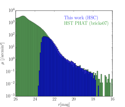
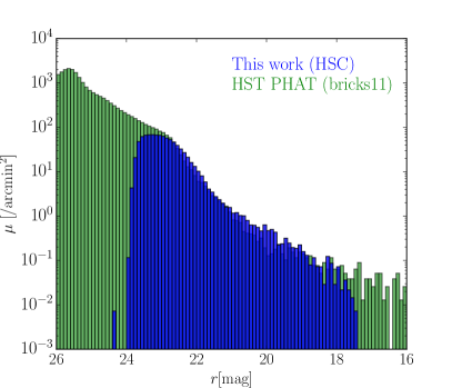
Fig. 23 compares the surface density of stars in the HST PHAT catalog with that of the HSC peaks, as a function of magnitudes, in the overlapping regions between our M31 data and HST PHAT. These regions correspond to “bricks07” and “bricks11”. The figure clearly shows that the HSC peak counts fairly well reproduces the HST results down to $r\sim 23~{}$mag. Since the HSC photometry of each peak should be contaminated by fluxes of neighboring stars, we would expect a systematic error in the PSF photometry, which causes a horizontal shift in the surface density of peaks (the HSC photometry is expected to over-estimate the magnitude). Even with this contamination, the agreement looks promising. However, it is clear that the HSC peak counts clearly misses the fainter stars, which can be potential source stars for PBH microlensing. The surface density of HST stars in different regions look similar.

The data overlap between HSC and PHAT covers the disk region only partially. Nevertheless, as an estimate of our star counts, we infer the underlying luminosity function of stars in the disk region from the HST PHAT catalog based on the number counts of HSC peaks at $m_{r}=23~{}$mag in each patch of the disk regions, assuming that the luminosity function of HST stars is universal in the disk regions. For the halo regions, we use the HSC peak counts. In this estimate of source stars, we find about $8.7\times 10^{7}$ stars down to $m_{r}=26~{}$mag over the entire region of M31, which is a factor of 14 more number of stars than that of HSC peaks. However, the source stars extrapolated from the HST data are faint, and will suffer from lower detection efficiency. Therefore, the final constraints do not improve a lot from these improved star counts.

One might worry about a possible contamination of dust extinction to the number counts of source stars. However our estimation of the source star counts is based on the HSC photometry that is already affected by dust extinction. Hence, we do not think that dust extinction largely affects the following results.

5 Discussion

Figure 24: The event rate of PBH microlensing for a single star in M31 when taking into account the effect of finite source size. Given the fact that the HSC data (down to $r\simeq 26$ mag) is sufficiently deep to reach main-sequence stars in M31, rather than red-giant branch stars, we assume a solar radius for source star size. The finite source size effect lowers the event rate compared to Fig. 8. The lower panel shows the relative contribution of PBHs in the MW or M31 halo region to the event rate for PBHs with $M_{\rm PBH}=10^{-8}M_{\odot}$. The upper thin solid curve is the result for a point source, the same as in the right panel of Fig. 8. The microlensing events in M31 are mainly from nearby PBHs to a source star at distance within a few tens of kpc (see Fig. 6), so the finite source size effect is more significant for such PBHs due to their relatively small Einstein radii.

Figure 25: The solid curve shows the 95% C.L. upper bound when ignoring the wave optics effect or equivalently taking into account only the effect of finite source size on the event rate of microlensing, assuming a solar radius for stars in M31. For comparison, the dotted curve shows the result for a point source, i.e. when ignoring both effects of the finite source size and the wave optics, while the dashed curve shows the results including both the effects, which is our default result shown in Fig. 5.

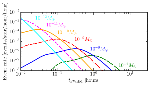
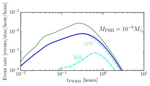
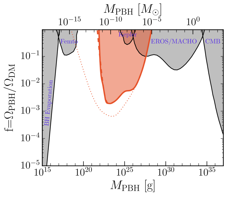
Although our results for the upper bounds in Fig. 5 are promising, we employed several assumptions. In this section, we discuss the impacts of our assumptions.

One uncertainty in our bounds comes from the number counts of source stars in M31, which is a result of blending of stars in the HSC data due to overcrowding, especially in the disk regions of M31. If we use the number of HSC peaks for the counts of source stars, $6.4\times 10^{6}$ instead of $8.7\times 10^{7}$, the counts extrapolated from the HST luminosity function, the upper bounds in Fig. 5 are weakened by a factor of 10. Nevertheless the upper bounds are quite tight, and very meaningful. However, we again stress that the use of HSC peak counts is extremely conservative, so we believe that our fiducial method using the HST-extrapolated counts of source stars is reasonable.

Another uncertainty in our analysis is the effect of finite source size. As can be found by comparing Eqs. (4) and (5), the angular size of the source star can be greater than the Einstein radius if PBHs are close to M31 or if PBHs are in the small mass range such of $M_{\rm PBH}\lower 2.15277pt\hbox{$\;\buildrel<\over{\sim}\;$}10^{-10}M_{\odot}$ (assuming solar radius for the star), all of which result in a smaller Einstein radius. Compared to the distance modulus for M31 is $\mu\simeq 24.4~{}$mag, our HSC depth is deep enough ($r\simeq 26~{}$mag) to reach main sequence stars whose absolute magnitudes $M_{r}\simeq 1.5$ mag. According to Figs. 23 and 24 in [31], most such faint stars at $r\sim 25$–26 mag would be either main sequence stars (probably A or F-type stars) or subgiant stars. In either case such stars have radii similar to the Sun within a factor of 2 or so [17]. The shallower data such as the work by [18] probes the microlensing events only for much brighter stars such as red giant branch (RGB) stars. RGB stars have much greater radius than that of main sequence stars, where the finite source size effect is more significant. Here we employ a solar radius ($R_{\odot}\simeq 6.96\times 10^{10}$ cm) for all source stars for simplicity, assuming that the upper bound is mainly from the microlensing for main sequence stars, rather than for RGB stars [31]. We followed [37] to re-estimate the event rates of PBHs microlensing taking into account the finite source size effect. Fig. 24 shows that the finite source size effect lowers the event rate, compared to Fig. 8. In particular the effect is greater for PBHs of smaller mass scales and in the M31 halo region.

For the results in Fig. 5, we also took into account the effect of wave optics. Since the Schwarzschild radii for light PBHs with $M\lower 2.15277pt\hbox{$\;\buildrel<\over{\sim}\;$}10^{-10}M_{\odot}$ become comparable with or smaller than the wavelength of the HSC $r$-band filter, the wave effect lowers the maximum magnification of the microlensing light curve [38, 39, 19]. The dashed curve in Fig. 25 shows the upper bounds when ignoring the wave effect or equivalently when including only the finite source size effect. As can be found the finite source size effect is a dominant effect compared to the wave effect, and the upper bounds are not largely different in the two cases. This confirms the recent study where the finite source size effect is more important for femtolensing of gamma ray bursts [20]. These finite source size and wave optics effects for microlensing searches need to be further carefully studied, and this is our future work.

Theory for PBH formation, via the nature of primordial fluctuations or the nonlinear collapse mechanism, predicts that PBHs generally have a mass spectrum, rather than the monochromatic spectrum. To compare models with non-monochromatic spectrum, our observed number of events should be compared to the events predicted using Eq. 1 further integrated over the PBH mass spectrum, i.e.,

$$N_{\rm exp}\!\left(\frac{\Omega_{\rm PBH}}{\Omega_{\rm DM}}\right)=\frac{\Omega_{\rm PBH}}{\Omega_{\rm DM}}\int{\rm d}M_{\rm PBH}\int_{0}^{t_{\rm obs}}\!\!\frac{\mathrm{d}t_{\rm FWHM}}{t_{\rm FWHM}}~{}\int\!\!\mathrm{d}m_{r}~{}\frac{\mathrm{d}N_{\rm event}}{\mathrm{d}{\ln t}_{\rm FWHM}}\frac{\mathrm{d}N_{s}}{\mathrm{d}m_{r}}\epsilon({t}_{\rm FWHM},m_{r})P(M_{\rm PBH}),$$ (26)

where $P(M_{\rm PBH})$ is a mass spectrum of PBHs, normalized so as to satisfy $\int_{0}^{\infty}\!\mathrm{d}M_{\rm PBH}~{}P(M_{\rm PBH})=1$. Then one can use our constraints to constrain the overall PBH mass fraction to DM, $\Omega_{\rm PBH}/\Omega_{\rm DM}$, following the method in Refs. [9, 21, 46, 47]).

Data availability

The catalog of variability star candidates including the candidates shown in this paper is available from the corresponding author upon reasonable request.

References

- [1] Davis, M., Efstathiou, G., Frenk, C. S. & White, S. D. M. The evolution of large-scale structure in a universe dominated by cold dark matter. Astrophys. J. 292, 371–394 (1985).
- [2] Clowe, D. et al. A Direct Empirical Proof of the Existence of Dark Matter. Astrophys. J. Lett. 648, L109–L113 (2006). astro-ph/0608407.
- [3] Dodelson, S. & Liguori, M. Can Cosmic Structure Form without Dark Matter? Phys. Rev. Lett. 97, 231301 (2006). astro-ph/0608602.
- [4] Jungman, G., Kamionkowski, M. & Griest, K. Supersymmetric dark matter. Phys. Rep. 267, 195–373 (1996). hep-ph/9506380.
- [5] Klasen, M., Pohl, M. & Sigl, G. Indirect and direct search for dark matter. Prog. Part. Nucl. Phys. 85, 1–32 (2015). 1507.03800.
- [6] Zel’dovich, Y. B. & Novikov, I. D. The Hypothesis of Cores Retarded during Expansion and the Hot Cosmological Model. Sov. Astron. 10, 602 (1967).
- [7] Hawking, S. Gravitationally collapsed objects of very low mass. Mon. Not. R. Astron. Soc. 152, 75 (1971).
- [8] Carr, B. J. & Hawking, S. W. Black holes in the early Universe. Mon. Not. R. Astron. Soc. 168, 399–416 (1974).
- [9] Carr, B., Kühnel, F. & Sandstad, M. Primordial black holes as dark matter. Phys. Rev. D 94, 083504 (2016). 1607.06077.
- [10] Capela, F., Pshirkov, M. & Tinyakov, P. Constraints on primordial black holes as dark matter candidates from capture by neutron stars. Phys. Rev. D 87, 123524 (2013). 1301.4984.
- [11] Lane, R. R. et al. Testing Newtonian gravity with AAOmega: mass-to-light profiles of four globular clusters. Mon. Not. R. Astron. Soc. 400, 917–923 (2009). 0908.0770.
- [12] Paczynski, B. Gravitational microlensing by the galactic halo. Astrophys. J. 304, 1–5 (1986).
- [13] Griest, K. et al. Gravitational microlensing as a method of detecting disk dark matter and faint disk stars. Astrophys. J. Lett. 372, L79–L82 (1991).
- [14] Alcock, C. et al. The MACHO Project: Microlensing Results from 5.7 Years of Large Magellanic Cloud Observations. Astrophys. J. 542, 281–307 (2000). astro-ph/0001272.
- [15] Tisserand, P. et al. Limits on the Macho content of the Galactic Halo from the EROS-2 Survey of the Magellanic Clouds. Astron. Astrophys. 469, 387–404 (2007). astro-ph/0607207.
- [16] Sasaki, M., Suyama, T., Tanaka, T. & Yokoyama, S. Primordial Black Hole Scenario for the Gravitational-Wave Event GW150914. Phys. Rev. Lett. 117, 061101 (2016). 1603.08338.
- [17] Ali-Haïmoud, Y., Kovetz, E. D. & Kamionkowski, M. The merger rate of primordial-black-hole binaries. ArXiv e-prints (2017). 1709.06576.
- [18] Griest, K., Cieplak, A. M. & Lehner, M. J. Experimental Limits on Primordial Black Hole Dark Matter from the First 2 yr of Kepler Data. Astrophys. J. 786, 158 (2014). 1307.5798.
- [19] Miyazaki, S. et al. Hyper Suprime-Cam: System design and verification of image quality. Pub. Astron. Soc. Jap. 70, S1 (2018).
- [20] Aihara, H. et al. First data release of the Hyper Suprime-Cam Subaru Strategic Program. Pub. Astron. Soc. Jap. 70, S8 (2018). 1702.08449.
- [21] Klypin, A., Zhao, H. & Somerville, R. S. CDM-based Models for the Milky Way and M31. I. Dynamical Models. Astrophys. J. 573, 597–613 (2002). astro-ph/0110390.
- [22] Aihara, H. et al. The Hyper Suprime-Cam SSP Survey: Overview and survey design. Pub. Astron. Soc. Jap. 70, S4 (2018). 1704.05858.
- [23] Crotts, A. P. S. M31 - A unique laboratory for gravitational microlensing. Astrophys. J. Lett. 399, L43–L46 (1992).
- [24] Baillon, P., Bouquet, A., Giraud-Heraud, Y. & Kaplan, J. Detection of Brown Dwarfs by the Microlensing of Unresolved Stars. Astron. Astrophys. 277, 1 (1993). astro-ph/9211002.
- [25] Gould, A. Theory of Pixel Lensing. Astrophys. J. 470, 201 (1996). astro-ph/9509009.
- [26] Calchi Novati, S. Pixel lensing. Microlensing towards M31. General Relativity and Gravitation 42, 2101–2126 (2010). 0912.2667.
- [27] Aurière, M. et al. A Short-Timescale Candidate Microlensing Event in the POINT-AGAPE Pixel Lensing Survey of M31. Astrophys. J. Lett. 553, L137–L140 (2001). astro-ph/0102080.
- [28] Alard, C. & Lupton, R. H. A Method for Optimal Image Subtraction. Astrophys. J. 503, 325–331 (1998). astro-ph/9712287.
- [29] Bosch, J. et al. The Hyper Suprime-Cam software pipeline. Pub. Astron. Soc. Jap. 70, S5 (2018). 1705.06766.
- [30] Williams, B. F. et al. The Panchromatic Hubble Andromeda Treasury. X. Ultraviolet to Infrared Photometry of 117 Million Equidistant Stars. Astrophys. J. Suppl. S. 215, 9 (2014). 1409.0899.
- [31] Dalcanton, J. J. et al. The Panchromatic Hubble Andromeda Treasury. Astrophys. J. Suppl. S. 200, 18 (2012). 1204.0010.
- [32] Carr, B. J., Kohri, K., Sendouda, Y. & Yokoyama, J. New cosmological constraints on primordial black holes. Phys. Rev. D 81, 104019 (2010). 0912.5297.
- [33] Barnacka, A., Glicenstein, J.-F. & Moderski, R. New constraints on primordial black holes abundance from femtolensing of gamma-ray bursts. Phys. Rev. D 86, 043001 (2012). 1204.2056.
- [34] Ali-Haïmoud, Y. & Kamionkowski, M. Cosmic microwave background limits on accreting primordial black holes. Phys. Rev. D 95, 043534 (2017). 1612.05644.
- [35] Ricotti, M., Ostriker, J. P. & Mack, K. J. Effect of Primordial Black Holes on the Cosmic Microwave Background and Cosmological Parameter Estimates. Astrophys. J. 680, 829–845 (2008). 0709.0524.
- [36] Huang, S. et al. Characterization and photometric performance of the Hyper Suprime-Cam Software Pipeline. Pub. Astron. Soc. Jap. 70, S6 (2018). 1705.01599.
- [37] Witt, H. J. & Mao, S. Can lensed stars be regarded as pointlike for microlensing by MACHOs? Astrophys. J. 430, 505–510 (1994).
- [38] Gould, A. Femtolensing of gamma-ray bursters. Astrophys. J. Lett. 386, L5–L7 (1992).
- [39] Nakamura, T. T. Gravitational Lensing of Gravitational Waves from Inspiraling Binaries by a Point Mass Lens. Phys. Rev. Lett. 80, 1138–1141 (1998).
- [40] Musco, I., Miller, J. C. & Polnarev, A. G. Primordial black hole formation in the radiative era: investigation of the critical nature of the collapse. Classical and Quantum Gravity 26, 235001 (2009). 0811.1452.
- [41] Kühnel, F., Rampf, C. & Sandstad, M. Effects of critical collapse on primordial black-hole mass spectra. European Physical Journal C 76, 93 (2016). 1512.00488.
- [42] Kawasaki, M., Mukaida, K. & Yanagida, T. T. Simple cosmological solution to the Higgs field instability problem in chaotic inflation and the formation of primordial black holes. Phys. Rev. D 94, 063509 (2016). 1605.04974.
- [43] Kawasaki, M., Kusenko, A., Tada, Y. & Yanagida, T. T. Primordial black holes as dark matter in supergravity inflation models. Phys. Rev. D 94, 083523 (2016). 1606.07631.
- [44] Inomata, K., Kawasaki, M., Mukaida, K., Tada, Y. & Yanagida, T. T. Inflationary primordial black holes for the LIGO gravitational wave events and pulsar timing array experiments. Phys. Rev. D 95, 123510 (2017). 1611.06130.
- [45] Kühnel, F. & Freese, K. Constraints on primordial black holes with extended mass functions. Phys. Rev. D 95, 083508 (2017). 1701.07223.
- [46] Inomata, K., Kawasaki, M., Mukaida, K., Tada, Y. & Yanagida, T. T. Inflationary primordial black holes as all dark matter. Phys. Rev. D 96, 043504 (2017). 1701.02544.
- [47] Carr, B., Raidal, M., Tenkanen, T., Vaskonen, V. & Veermäe, H. Primordial black hole constraints for extended mass functions. Phys. Rev. D 96, 023514 (2017). 1705.05567.
- [1] Alcock, C., et al., The MACHO Project First-Year Large Magellanic Cloud Results: The Microlensing Rate and the Nature of the Galactic Dark Halo. Astrophys. J., 461, 84 (1996).
- [2] Kerins, E. et al., Theory of pixel lensing towards M31 - I. The density contribution and mass of MACHOs. Mon. Not. R. Astron. Soc., 323, 13 (2001).
- [3] Riffeser, A., Fliri, J., Seitz, S. & Bender, R., Microlensing toward Crowded Fields: Theory and Applications to M31. Astrophys. J. Suppl. S., 163, 225 (2006).
- [4] Cieplak, A. M. & Griest, K., Improved Theoretical Predictions of Microlensing Rates for the Detection of Primordial Black Hole Dark Matter. Astrophys. J., 767, 145 (2013).
- [5] Navarro, J. F., Frenk, C. S. & White, S. D. M., A Universal Density Profile from Hierarchical Clustering. Astrophys. J., 490, 493 (1997).
- [6] Gondolo, P., Optical Depth Evaluation in Pixel Microlensing. Astrophys. J. Lett., 510, L29 (1999).
- [7] Ivezic, Z. et al., LSST: from Science Drivers to Reference Design and Anticipated Data Products. ArXiv e-prints:0805.2366 .
- [8] Axelrod, T., Kantor, J., Lupton, R. H. & Pierfederici, F., An open source application framework for astronomical imaging pipelines. Software and Cyberinfrastructure for Astronomy, vol. 7740 of Proceedings of the SPIE, 774015 (2010).
- [9] Jurić, M. et al., The LSST Data Management System. ArXiv e-prints:1512.07914 .
- [10] Bertin, E., Automated Morphometry with SExtractor and PSFEx. In Evans, I. N., Accomazzi, A., Mink, D. J. & Rots, A. H. (eds.) Astronomical Data Analysis Software and Systems XX, vol. 442 of Astronomical Society of the Pacific Conference Series, 435 (2011).
- [11] Schlafly, E. F. et al., Photometric Calibration of the First 1.5 Years of the Pan-STARRS1 Survey. Astrophys. J., 756, 158 (2012).
- [12] Tonry, J. L. et al., The Pan-STARRS1 Photometric System. Astrophys. J., 750, 99 (2012).
- [13] Magnier, E. A. et al., The Pan-STARRS 1 Photometric Reference Ladder, Release 12.01. Astrophys. J. Suppl. S., 205, 20 (2013).
- [14] Alard, C., Image subtraction using a space-varying kernel. Astron. Astrophys. Supp., 144, 363 (2000).
- [15] Mandelbaum, R. et al., The Third Gravitational Lensing Accuracy Testing (GREAT3) Challenge Handbook. Astrophys. J. Suppl. S., 212, 5 (2014).
- [16] Rowe, B. T. P. et al., GALSIM: The modular galaxy image simulation toolkit. Astronomy and Computing, 10, 121 (2015).
- [17] North, J. R. et al., The radius and mass of the subgiant star Hyi from interferometry and asteroseismology. Mon. Not. R. Astron. Soc., 380, L80 (2007).
- [18] de Jong, J. T. A. et al., MACHOs in M 31? Absence of evidence but not evidence of absence. Astron. Astrophys., 446, 855 (2006).
- [19] Takahashi, R. & Nakamura, T., Wave Effects in the Gravitational Lensing of Gravitational Waves from Chirping Binaries. Astrophys. J., 595, 1039 (2003).
- [20] Katz, A., Kopp, J., Sibiryakov, S. & Xue, W., Femtolensing by Dark Matter Revisited. ArXiv e-prints:1807.11495 .
- [21] Green, A. M., Microlensing and dynamical constraints on primordial black hole dark matter with an extended mass function. Phys. Rev. D, 94, 063530 (2016).