Learning Locomotion Skills Using DeepRL:
Does the Choice of Action Space Matter?

Abstract

The use of deep reinforcement learning allows for high-dimensional state descriptors, but little is known about how the choice of action representation impacts the learning difficulty and the resulting performance. We compare the impact of four different action parameterizations (torques, muscle-activations, target joint angles, and target joint-angle velocities) in terms of learning time, policy robustness, motion quality, and policy query rates. Our results are evaluated on a gait-cycle imitation task for multiple planar articulated figures and multiple gaits. We demonstrate that the local feedback provided by higher-level action parameterizations can significantly impact the learning, robustness, and quality of the resulting policies.

1 Introduction

The introduction of deep learning models to reinforcement learning (RL) has enabled policies to operate directly on high-dimensional, low-level state features. As a result, deep reinforcement learning (DeepRL) has demonstrated impressive capabilities, such as developing control policies that can map from input image pixels to output joint torques  (Lillicrap et al., 2015). However, the quality and robustness often falls short of what has been achieved with hand-crafted action abstractions, e.g., Coros et al. (2011); Geijtenbeek et al. (2013). Relatedly, the choice of action parameterization is a design decision whose impact is not yet well understood.

Joint torques can be thought of as the most basic and generic representation for driving the movement of articulated figures, given that muscles and other actuation models eventually result in joint torques. However this ignores the intrinsic embodied nature of biological systems, particularly the synergy between control and biomechanics. Passive-dynamics, such as elasticity and damping from muscles and tendons, play an integral role in shaping motions: they provide mechanisms for energy storage, and mechanical impedance which generates instantaneous feedback without requiring any explicit computation. Loeb coins the term preflexes (Loeb, 1995) to describe these effects, and their impact on motion control has been described as providing intelligence by mechanics (Blickhan et al., 2007).

In this paper we explore the impact of four different actuation models on learning to control dynamic articulated figure locomotion: (1) torques (Tor); (2) activations for musculotendon units (MTU); (3) target joint angles for proportional-derivative controllers (PD); and (4) target joint velocities (Vel). Because Deep RL methods are capable of learning control policies for all these models, it now becomes possible to directly assess how the choice of actuation model affects the learning difficulty. We also assess the learned policies with respect to robustness, motion quality, and policy query rates. We show that action spaces which incorporate local feedback can significantly improve learning speed and performance, while still preserving the generality afforded by torque-level control. Such parameterizations also allow for more complex body structures and subjective improvements in motion quality.

Our specific contributions are: (1) We introduce a DeepRL framework for motion imitation tasks; (2) We evaluate the impact of four different actuation models on learned control policies according to four criteria; and (3) We propose an optimization approach that combines policy learning and actuator optimization, allowing neural networks to effective control complex muscle models.

2 Background

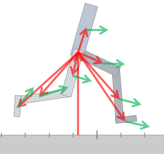
Our task will be structured as a standard reinforcement problem where an agent interacts with its environment according to a policy in order to maximize a reward signal. The policy $\pi(s,a)=p(a|s)$ represents the conditional probability density function of selecting action $a\in\mathcal{A}$ in state $s\in\mathcal{S}$. At each control step $t$, the agent observes a state $s_{t}$ and samples an action $a_{t}$ from $\pi$. The environment in turn responds with a scalar reward $r_{t}$, and a new state $s^{\prime}_{t}=s_{t+1}$ sampled from its dynamics $p(s^{\prime}|s,a)$. For a parameterized policy $\pi_{\theta}(s,a)$, the goal of the agent is learn the parameters $\theta$ which maximizes the expected cumulative reward

$$J(\pi_{\theta})=\mathop{\mathbb{E}}\left[\sum_{t=0}^{T}\gamma^{t}r_{t}\middle|\pi_{\theta}\right]$$

with $\gamma\in[0,1]$ as the discount factor, and $T$ as the horizon. The gradient of the expected reward $\triangledown_{\theta}J(\pi_{\theta})$ can be determined according to the policy gradient theorem (Sutton et al., 2001), which provides a direction of improvement to adjust the policy parameters $\theta$.

$$\triangledown_{\theta}J(\pi_{\theta})=\int_{\mathcal{S}}d_{\theta}(s)\int_{\mathcal{A}}\triangledown_{\theta}\mathrm{log}(\pi_{\theta}(s,a))A(s,a)da\ ds$$

where $d_{\theta}(s)=\int_{\mathcal{S}}\sum_{t=0}^{T}\gamma^{t}p_{0}(s_{0})p(s_{0}\rightarrow s|t,\pi_{\theta})ds_{0}$ is the discounted state distribution, where $p_{0}(s)$ represents the initial state distribution, and $p(s_{0}\rightarrow s|t,\pi_{\theta})$ models the likelihood of reaching state $s$ by starting at $s_{0}$ and following the policy $\pi_{\theta}(s,a)$ for $t$ steps (Silver et al., 2014). $A(s,a)$ represents a generalized advantage function. The choice of advantage function gives rise to a family of policy gradient algorithms, but in this work, we will focus on the one-step temporal difference advantage function (Schulman et al., 2015)

$$A(s_{t},a_{t})=r_{t}+\gamma V(s^{\prime}_{t})-V(s_{t})$$

where $V(s)=\mathop{\mathbb{E}}\left[\sum_{t=0}^{T}\gamma^{t}r_{t}\middle|s_{0}=s,\pi_{\theta}\right]$ is the state-value function, and can be defined recursively via the Bellman equation

$$V(s_{t})=\mathop{\mathbb{E}}_{r_{t},s^{\prime}_{t}}\left[r_{t}+\gamma V(s^{\prime}_{t})\middle|s_{t},\pi_{\theta}\right]$$

A parameterized value function $V_{\phi}(s)$, with parameters $\phi$, can be learned iteratively in a manner similar to Q-Learning by minimizing the Bellman loss,

$$L(\phi)=\mathop{\mathbb{E}}_{s_{t},r_{t},s^{\prime}_{t}}\left[\frac{1}{2}\left(y_{t}-V_{\phi}(s_{t})\right)^{2}\right],\qquad y_{t}=r_{t}+\gamma V_{\phi}(s^{\prime}_{t})$$

$\pi_{\theta}$ and $V_{\phi}$ can be trained in tandem using an actor-critic framework (Konda & Tsitsiklis, 2000).

In this work, each policy will be represented as a gaussian distribution with a parameterized mean $\mu_{\theta}(s)$ and fixed covariance matrix $\Sigma=\mathrm{diag}\{\sigma_{i}^{2}\}$, where $\sigma_{i}$ is manually specified for each action parameter. Actions can be sampled from the distribution by applying gaussian noise to the mean action

$$a_{t}=\mu_{\theta}(s_{t})+\mathcal{N}(0,\Sigma)$$

The corresponding policy gradient will assume the form

$$\triangledown_{\theta}J(\pi_{\theta})=\int_{\mathcal{S}}d_{\theta}(s)\int_{\mathcal{A}}\triangledown_{\theta}\mu_{\theta}(s)\Sigma^{-1}\left(a-\mu_{\theta}(s)\right)A(s,a)da\ ds$$

which can be interpreted as shifting the mean of the action distribution towards actions that lead to higher than expected rewards, while moving away from actions that lead to lower than expected rewards.

3 Task Representation

3.1 Reference Motion

In our task, the goal of a policy is to imitate a given reference motion $\{q^{*}_{t}\}$ which consists of a sequence of kinematic poses $q^{*}_{t}$ in reduced coordinates. The reference velocity $\dot{q^{*}_{t}}$ at a given time $t$ is approximated by finite-difference $\dot{q^{*}_{t}}\approx\frac{q^{*}_{t+\triangle t}-q^{*}_{t}}{\triangle t}$. Reference motions are generated via either using a recorded simulation result from a preexisting controller (“Sim”), or via manually-authored keyframes. Since hand-crafted reference motions may not be physically realizable, the goal is to closely reproduce a motion while satisfying physical constraints.

3.2 States

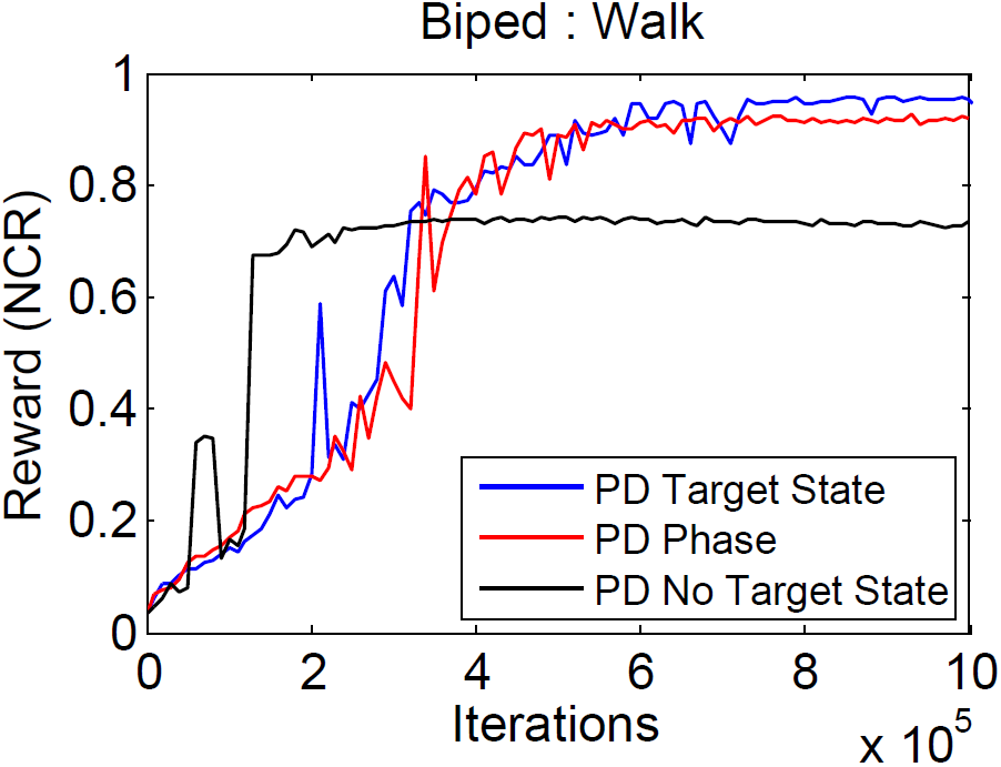
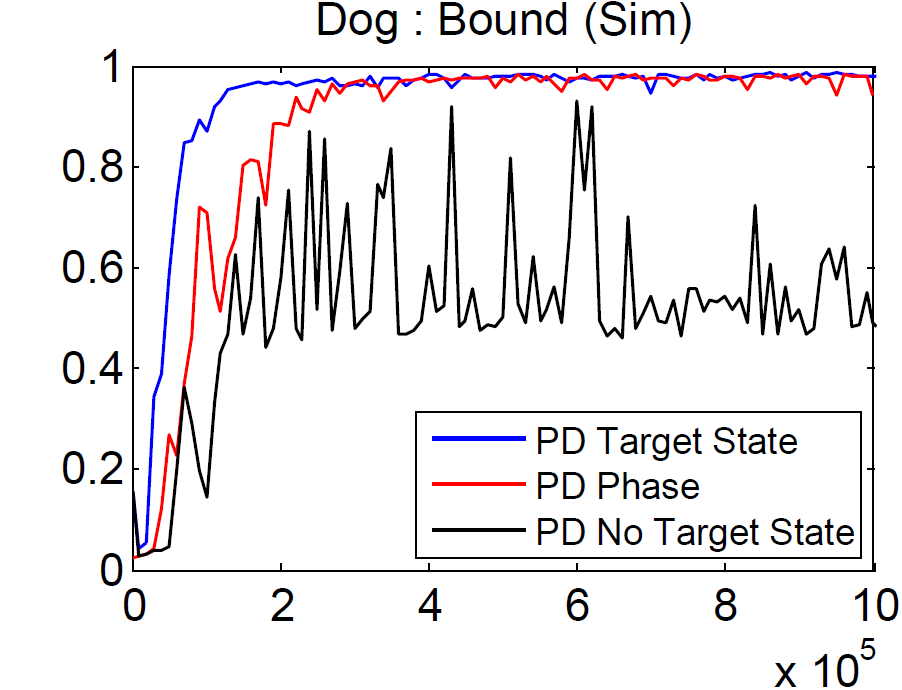
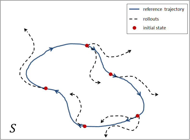
To define the state of the agent, a feature transformation $\Phi(q,\dot{q})$ is used to extract a set of features from the reduced-coordinate pose $q$ and velocity $\dot{q}$. The features consist of the height of the root (pelvis) from the ground, the position of each link with respect to the root, and the center of mass velocity of each link. When training a policy to imitate a cyclic reference motion $\{q_{t}^{*}\}$, knowledge of the motion phase can help simplify learning. Therefore, we augment the state features with a set of target features $\Phi(q_{t}^{*},\dot{q_{t}}^{*})$, resulting in a combined state represented by $s_{t}=(\Phi(q_{t},\dot{q_{t}}),\Phi(q_{t}^{*},\dot{q_{t}}^{*}))$. Similar results can also be achieved by providing a single motion phase variable as a state feature, as we show in Figure 12 (supplemental material).

3.3 Actions

We train separate policies for each of the four actuation models, as described below. Each actuation model also has related actuation parameters, such as feedback gains for PD-controllers and musculotendon properties for MTUs. These parameters can be manually specified, as we do for the PD and Vel models, or they can be optimized for the task at hand, as for the MTU models. Table 1 provides a list of actuator parameters for each actuation model.

Target Joint Angles (PD): Each action represents a set of target angles $\hat{q}$, where $\hat{q}^{i}$ specifies the target angles for joint $i$. $\hat{q}$ is applied to PD-controllers which compute torques according to $\tau^{i}=k_{p}^{i}(\hat{q}^{i}-q^{i})+k^{i}_{d}(\hat{\dot{q}}^{i}-\dot{q}^{i})$, where $\hat{\dot{q}}^{i}=0$, and $k_{p}^{i}$ and $k_{d}^{i}$ are manually-specified gains.

Target Joint Velocities (Vel): Each action specifies a set of target velocities $\hat{\dot{q}}$ which are used to compute torques according to $\tau^{i}=k_{d}^{i}(\hat{\dot{q}}^{i}-\dot{q}^{i})$, where the gains $k_{d}^{i}$ are specified to be the same as those used for target angles.

Torques (Tor): Each action directly specifies torques for every joint, and constant torques are applied for the duration of a control step. Due to torque limits, actions are bounded by manually specified limits for each joint. Unlike the other actuation models, the torque model does not require additional actuator parameters, and can thus be regarded as requiring the least amount of domain knowledge. Torque limits are excluded from the actuator parameter set as they are common for all parameterizations.

Muscle Activations (MTU): Each action specifies activations for a set of musculotendon units (MTU). Detailed modeling and implementation information are available in Wang et al. (2012). Each MTU is modeled as a contractile element (CE) attached to a serial elastic element (SE) and parallel elastic element (PE). The force exerted by the MTU can be calculated according to $F_{MTU}=F_{SE}=F_{CE}+F_{PE}$. Both $F_{SE}$ and $F_{PE}$ are modeled as passive springs, while $F_{CE}$ is actively controlled according to $F_{CE}=a_{MTU}F_{0}f_{l}(l_{CE})f_{v}(v_{CE})$, with $a_{MTU}$ being the muscle activation, $F_{0}$ the maximum isometric force, $l_{CE}$ and $v_{CE}$ being the length and velocity of the contractile element. The functions $f_{l}(l_{CE})$ and $f_{v}(v_{CE})$ represent the force-length and force-velocity relationships, modeling the variations in the maximum force that can be exerted by a muscle as a function of its length and contraction velocity. Analytic forms are available in Geyer et al. (2003). Activations are bounded between [0, 1]. The length of each contractile element $l_{CE}$ are included as state features. To simplify control and reduce the number of internal state parameters per MTU, the policies directly control muscle activations instead of indirectly through excitations (Wang et al., 2012).

Actuation Model	Actuator Parameters
Target Joint Angles (PD)	proportional gains $k_{p}$, derivative gains $k_{d}$
Target Joint Velocities (Vel)	derivative gains $k_{d}$
Torques (Tor)	none
Muscle Activations (MTU)	optimal contractile element length, serial elastic element rest length,
	maximum isometric force, pennation, moment arm,
	maximum moment arm joint orientation, rest joint orientation.

Table 1: Actuation models and their respective actuator parameters.

3.4 Reward

The reward function consists of a weighted sum of terms that encourage the policy to track a reference motion.

$$r=w_{pose}r_{pose}+w_{vel}r_{vel}+w_{end}r_{end}+w_{root}r_{root}+w_{com}r_{com}$$

$$w_{pose}=0.5,\ w_{vel}=0.05,\ w_{end}=0.15,\ w_{root}=0.1,\ w_{com}=0.2$$

Details of each term are available in the supplemental material. $r_{pose}$ penalizes deviation of the character pose from the reference pose, and $r_{vel}$ penalizes deviation of the joint velocities. $r_{end}$ and $r_{root}$ accounts for the position error of the end-effectors and root. $r_{com}$ penalizes deviations in the center of mass velocity from that of the reference motion.

3.5 Initial State Distribution

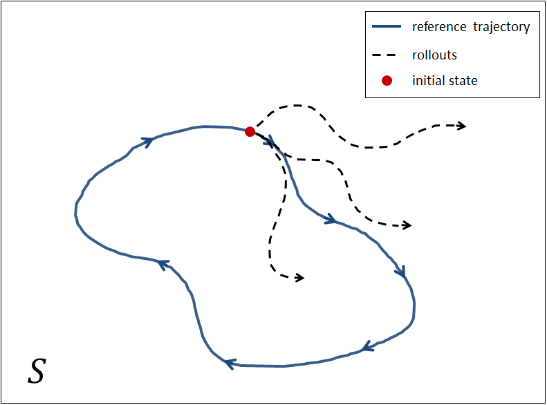
We design the initial state distribution, $p_{0}(s)$, to sample states uniformly along the reference trajectory. At the start of each episode, $q^{*}$ and $\dot{q}^{*}$ are sampled from the reference trajectory, and used to initialize the pose and velocity of the agent. This helps guide the agent to explore states near the target trajectory.

4 Actor-Critic Learning Algorithm

Instead of directly using the temporal difference advantage function, we adapt a positive temporal difference (PTD) update as proposed by Van Hasselt (2012).

$$A(s,a)=I\left[\delta>0\right]=\begin{cases}1,&\text{$\delta>0$}\\ 0,&\text{otherwise}\end{cases}$$

$$\delta=r+\gamma V(s^{\prime})-V(s)$$

Unlike more conventional policy gradient methods, PTD is less sensitive to the scale of the advantage function and avoids instabilities that can result from negative TD updates. For a Gaussian policy, a negative TD update moves the mean of the distribution away from an observed action, effectively shifting the mean towards an unknown action that may be no better than the current mean action (Van Hasselt, 2012). In expectation, these updates converges to the true policy gradient, but for stochastic estimates of the policy gradient, these updates can cause the agent to adopt undesirable behaviours which affect subsequent experiences collected by the agent. Furthermore, we incorporate experience replay, which has been demonstrated to improve stability when training neural network policies with Q-learning in discrete action spaces. Experience replay often requires off-policy methods, such as importance weighting, to account for differences between the policy being trained and the behavior policy used to generate experiences (WawrzyńSki & Tanwani, 2013). However, we have not found importance weighting to be beneficial for PTD.

Stochastic policies are used during training for exploration, while deterministic policy are deployed for evaluation at runtime. The choice between a stochastic and deterministic policy can be specified by the addition of a binary indicator variable $\lambda\in[0,1]$

$$a_{t}=\mu_{\theta}(s_{t})+\lambda\mathcal{N}(0,\Sigma)$$

where $\lambda=1$ corresponds to a stochastic policy with exploration noise, and $\lambda=0$ corresponds to a deterministic policy that always selects the mean of the distribution. Noise from a stochastic policy will result in a state distribution that differs from that of the deterministic policy at runtime. To imitate this discrepancy, we incorporate $\epsilon$-greedy exploration in addition to the original Gaussian exploration. During training, $\lambda$ is determined by a Bernoulli random variable $\lambda\sim\mathrm{Ber}(\epsilon)$, where $\lambda=1$ with probability $\epsilon\in[0,1]$. The exploration rate $\epsilon$ is annealed linearly from 1 to 0.2 over 500k iterations, which slowly adjusts the state distribution encountered during training to better resemble the distribution at runtime. Since the policy gradient is defined for stochastic policies, only tuples recorded with exploration noise (i.e. $\lambda=1$) can be used to update the actor, while the critic can be updated using all tuples.

Training proceeds episodically, where the initial state of each episode is sampled from $p_{0}(s)$, and the episode duration is drawn from an exponential distribution with a mean of 2s. To discourage falling, an episode will also terminate if any part of the character’s trunk makes contact with the ground for an extended period of time, leaving the agent with zero reward for all subsequent steps. Algorithm 1 in the supplemental material summarizes the complete learning process.

MTU Actuator Optimization: Actuation models such as MTUs are defined by further parameters whose values impact performance (Geijtenbeek et al., 2013). Geyer et al. (2003) uses existing anatomical estimates for humans to determine MTU parameters, but such data is not be available for more arbitrary creatures. Alternatively, Geijtenbeek et al. (2013) uses covariance matrix adaptation (CMA), a derivative-free evolutionary search strategy, to simultaneously optimize MTU and policy parameters. This approach is limited to policies with reasonably low dimensional parameter spaces, and is thus ill-suited for neural network models with hundreds of thousands of parameters. To avoid manual-tuning of actuator parameters, we propose a heuristic approach that alternates between policy learning and actuator optimization, as detailed in the supplemental material.

Figure 1: Simulated articulated figures and their state representation. Revolute joints connect all links. From left to right: 7-link biped; 19-link raptor; 21-link dog; State features: root height, relative position (red) of each link with respect to the root and their respective linear velocity (green).

Figure 2: Learning curves for each policy during 1 million iterations.

5 Results

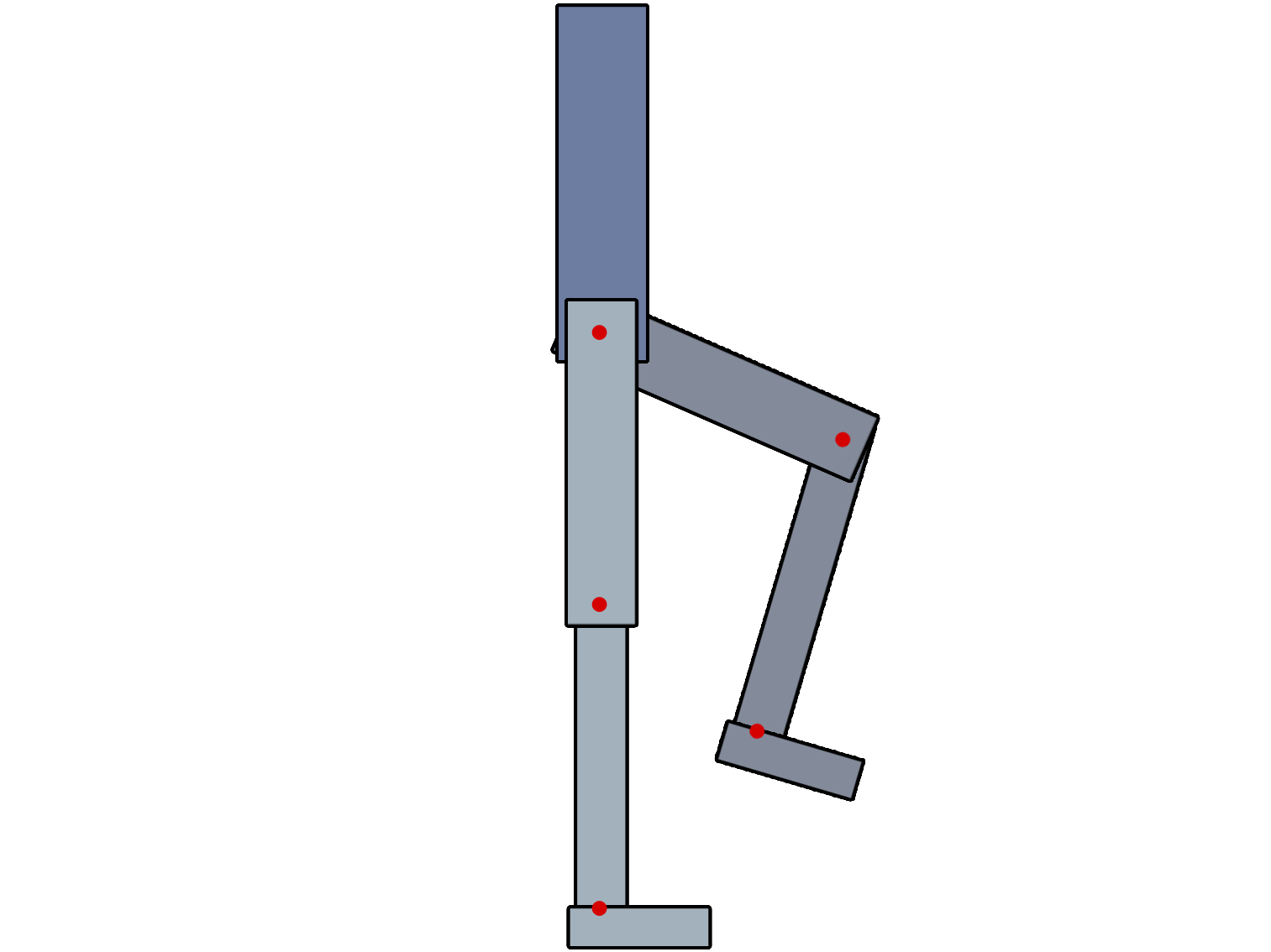
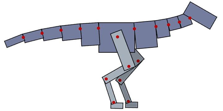
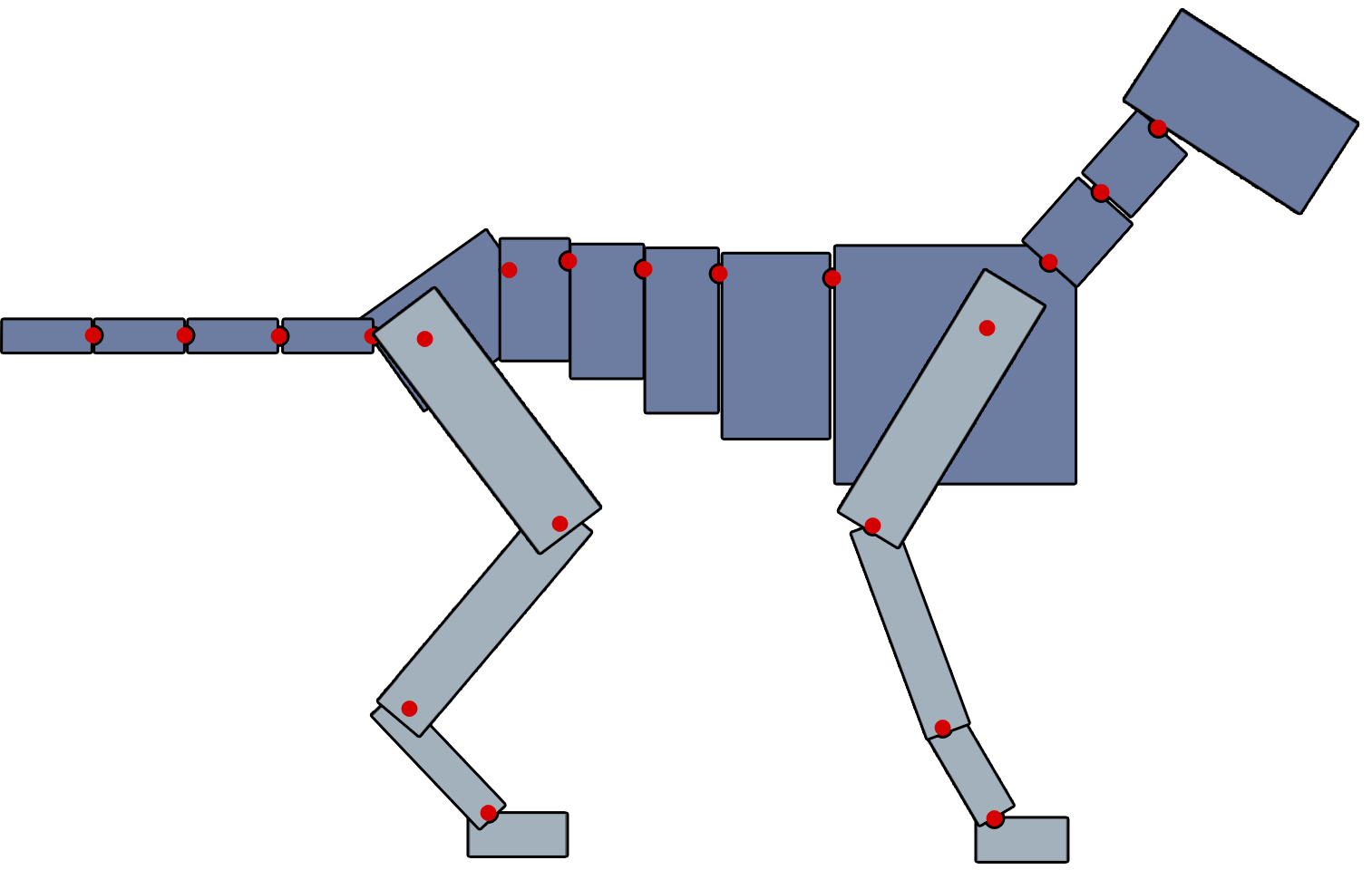
The motions are best seen in the supplemental video https://youtu.be/L3vDo3nLI98. We evaluate the action parameterizations by training policies for a simulated 2D biped, dog, and raptor as shown in Figure 1. Depending on the agent and the actuation model, our systems have 58–214 state dimensions, 6–44 action dimensions, and 0–282 actuator parameters, as summarized in Table 3 (supplemental materials). The MTU models have at least double the number of action parameters because they come in antagonistic pairs. As well, additional MTUs are used for the legs to more accurately reflect bipedal biomechanics. This includes MTUs that span multiple joints.

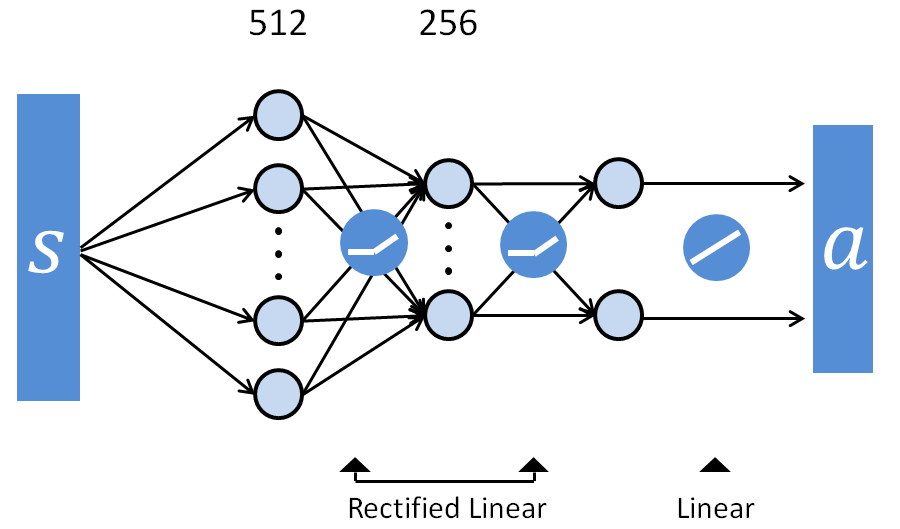
Each policy is represented by a three layer neural network, as illustrated in Figure 8 (supplemental material) with 512 and 256 fully-connected units, followed by a linear output layer where the number of output units vary according to the number of action parameters for each character and actuation model. ReLU activation functions are used for both hidden layers. Each network has approximately 200k parameters. The value function is represented by a similar network, except having a single linear output unit. The policies are queried at 60Hz for a control step of about 0.0167s. Each network is randomly initialized and trained for about 1 million iterations, requiring 32 million tuples, the equivalent of approximately 6 days of simulated time. Each policy requires about 10 hours for the biped, and 20 hours for the raptor and dog on an 8-core Intel Xeon E5-2687W.

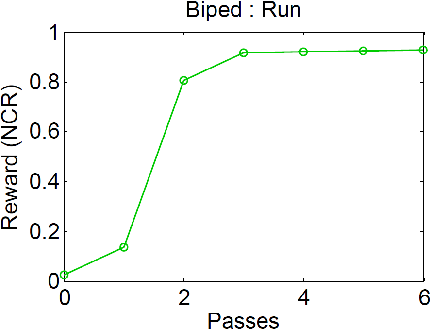
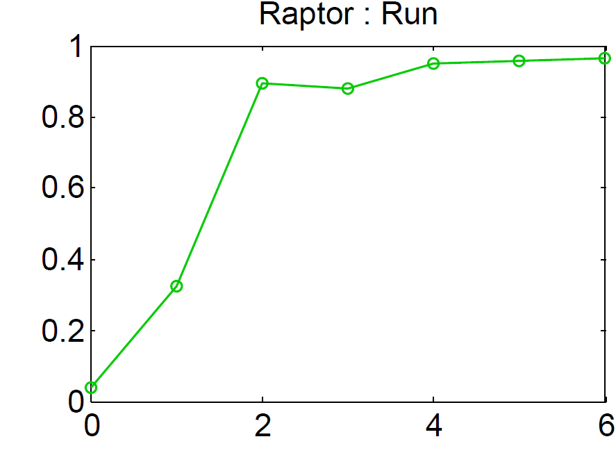
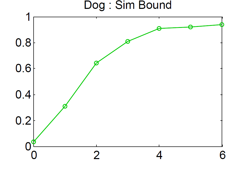
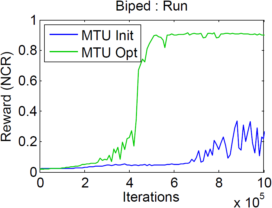
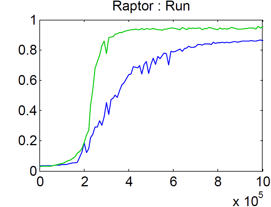
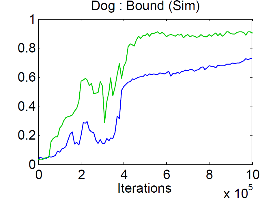
Only the actuator parameters for MTUs are optimized with Algorithm 2, since the parameters for the other actuation models are few and reasonably intuitive to determine. The initial actuator parameters $\psi_{0}$ are manually specified, while the initial policy parameters $\theta_{0}$ are randomly initialized. Each pass optimizes $\psi$ using CMA for 250 generations with 16 samples per generation, and $\theta$ is trained for 250k iterations. Parameters are initialized with values from the previous pass. The expected value of each CMA sample of $\psi$ is estimated using the average cumulative reward over 16 rollouts with a duration of 10s each. Separate MTU parameters are optimized for each character and motion. Each set of parameters is optimized for 6 passes following Algorithm 2, requiring approximately 50 hours. Figure 5 illustrates the performance improvement per pass. Figure 6 compares the performance of MTUs before and after optimization. For most examples, the optimized actuator parameters significantly improve learning speed and final performance. For the sake of comparison, after a set of actuator parameters has been optimized, a new policy is retrained with the new actuator parameters and its performance compared to the other actuation models.

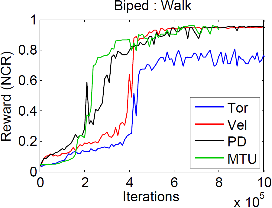
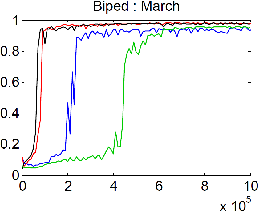
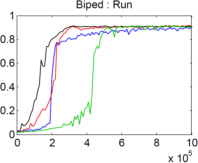
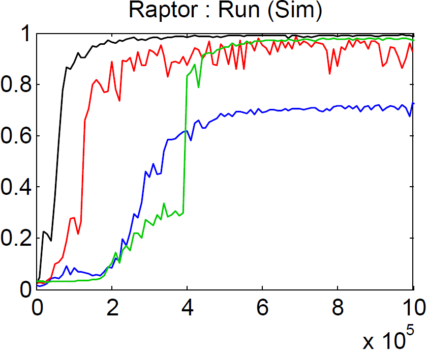
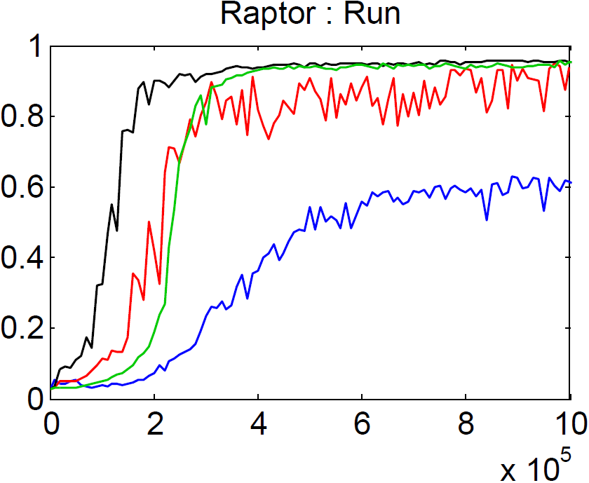
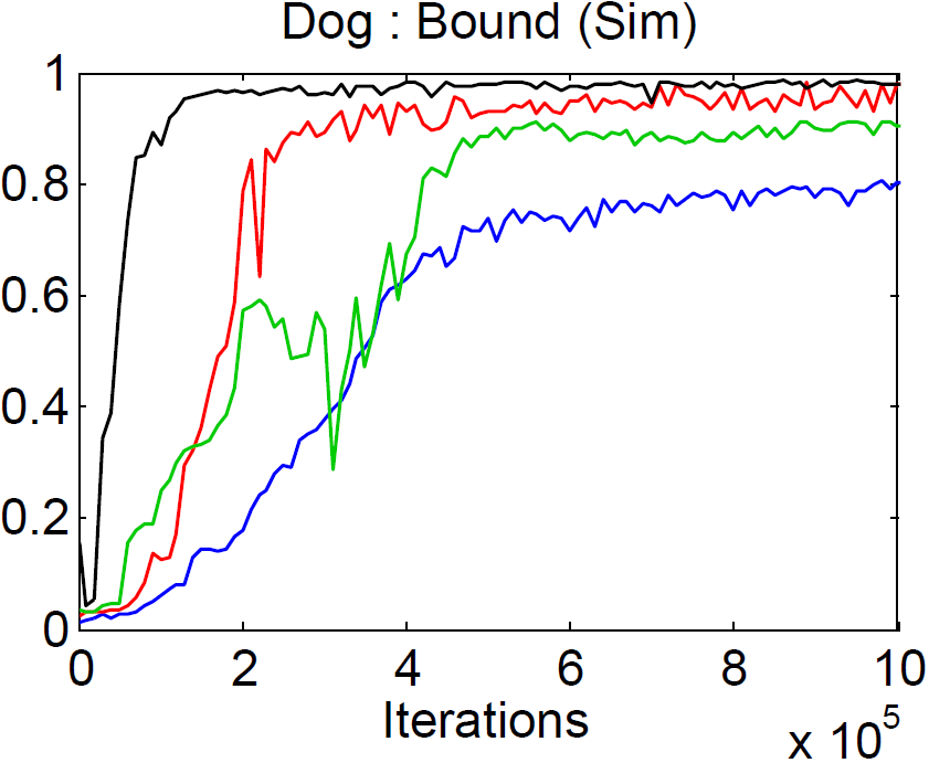
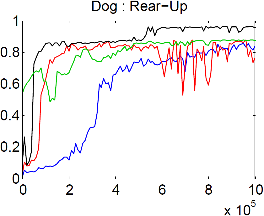
Policy Performance and Learning Speed: Figure 2 shows learning curves for the policies and the performance of the final policies are summarized in Table 4. Performance is evaluated using the normalized cumulative reward (NCR), calculated from the average cumulative reward over 32 episodes with lengths of 10s, and normalized by the maximum and minimum cumulative reward possible for each episode. No discounting is applied when calculating the NCR. The initial state of each episode is sampled from the reference motion according to $p(s_{0})$. To compare learning speeds, we use the normalized area under each learning curve (AUC) as a proxy for the learning speed of a particular actuation model, where 0 represents the worst possible performance and no progress during training, and 1 represents the best possible performance without requiring training.

PD performs well across all examples, achieving comparable-to-the-best performance for all motions. PD also learns faster than the other parameterizations for 5 of the 7 motions. The final performance of Tor is among the poorest for all the motions. Differences in performance appear more pronounced as characters become more complex. For the simple 7-link biped, most parameterizations achieve similar performance. However, for the more complex dog and raptor, the performance of Tor policies deteriorate with respect to other policies such as PD and Vel. MTU policies often exhibited the slowest learning speed, which may be a consequence of the higher dimensional action spaces, i.e., requiring antagonistic muscle pairs, and complex muscle dynamics. Nonetheless, once optimized, the MTU policies produce more natural motions and responsive behaviors as compared to other parameterizations. We note that the naturalness of motions is not well captured by the reward, since it primarily gauges similarity to the reference motion, which may not be representative of natural responses when perturbed from the nominal trajectory.

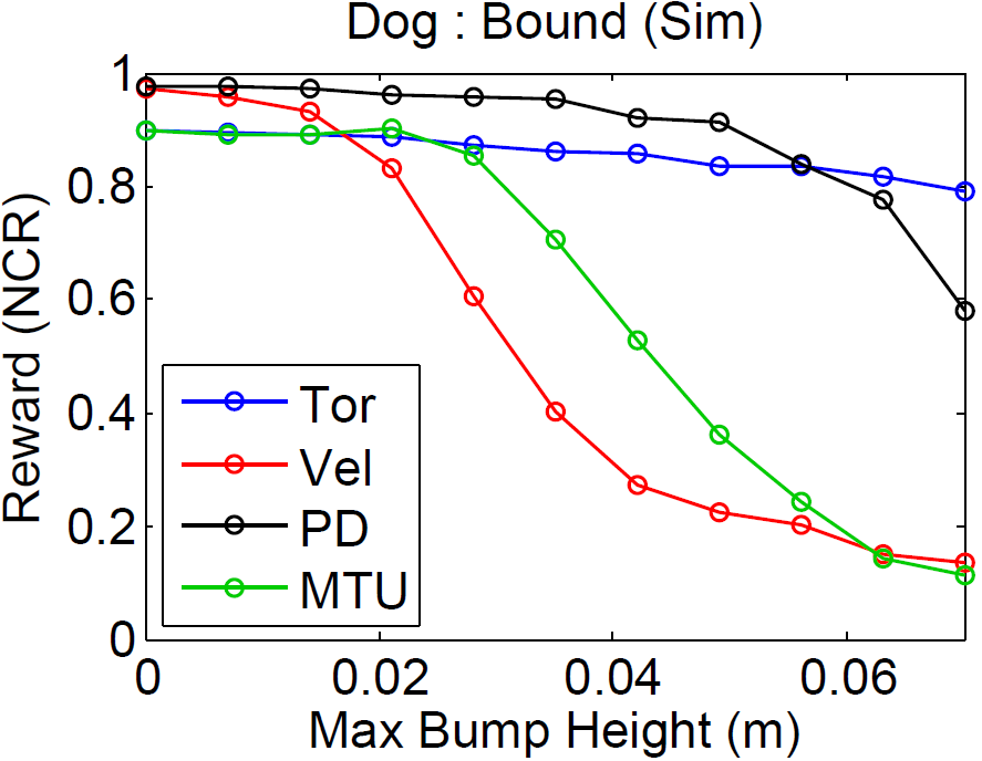
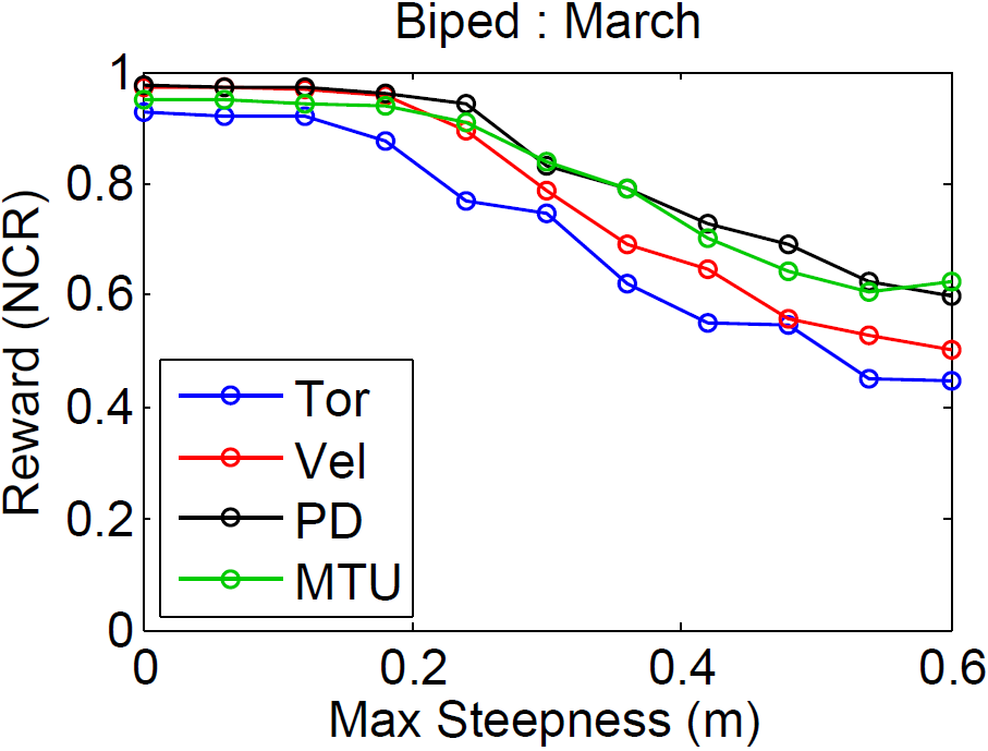
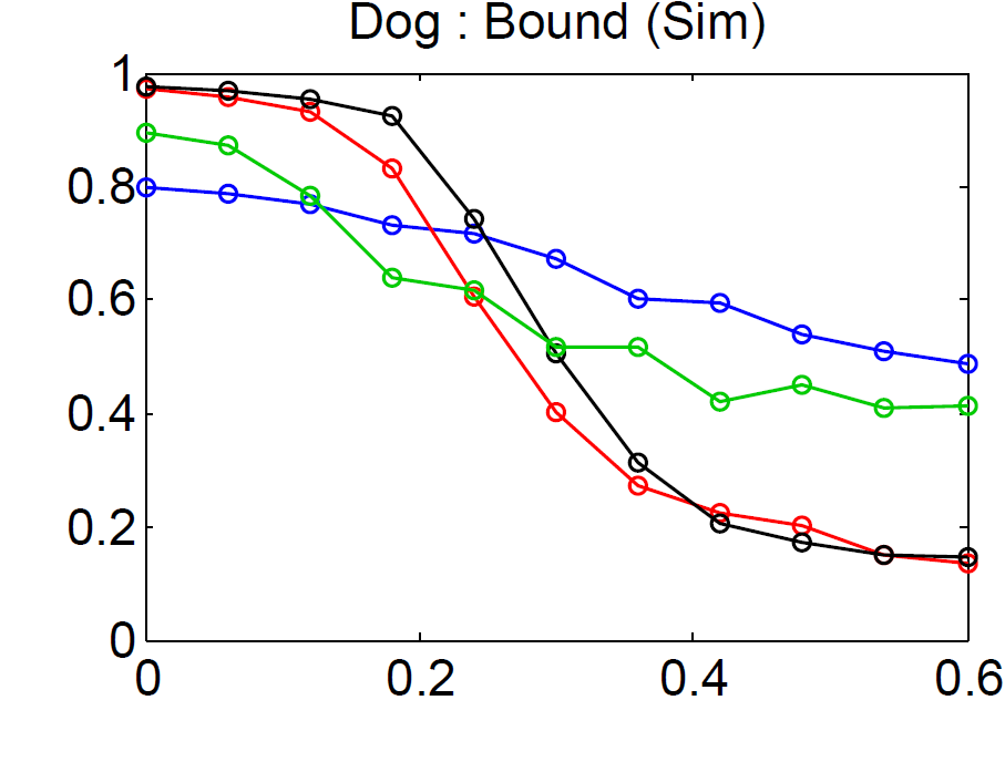
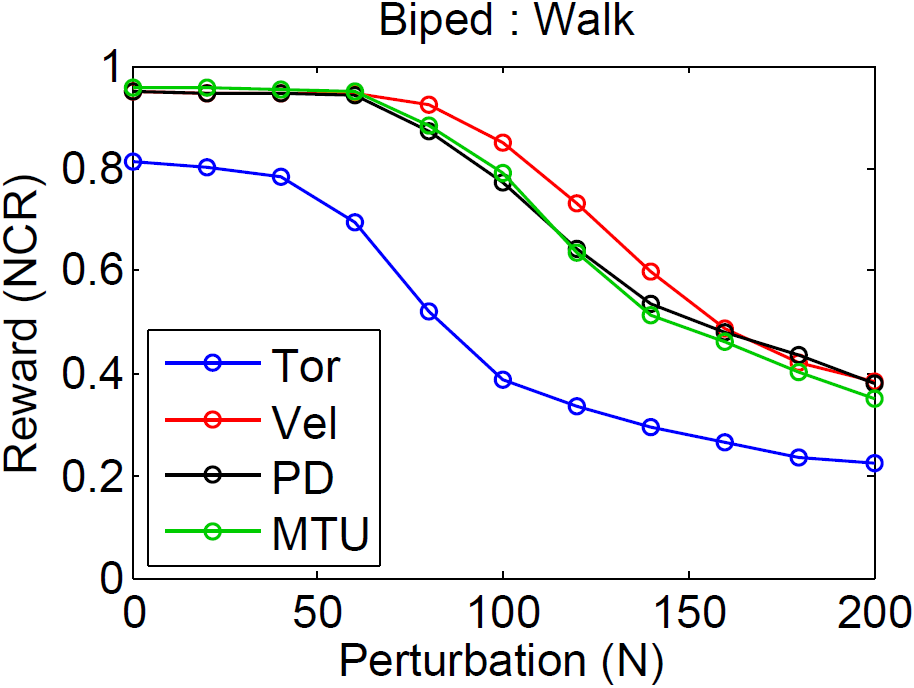
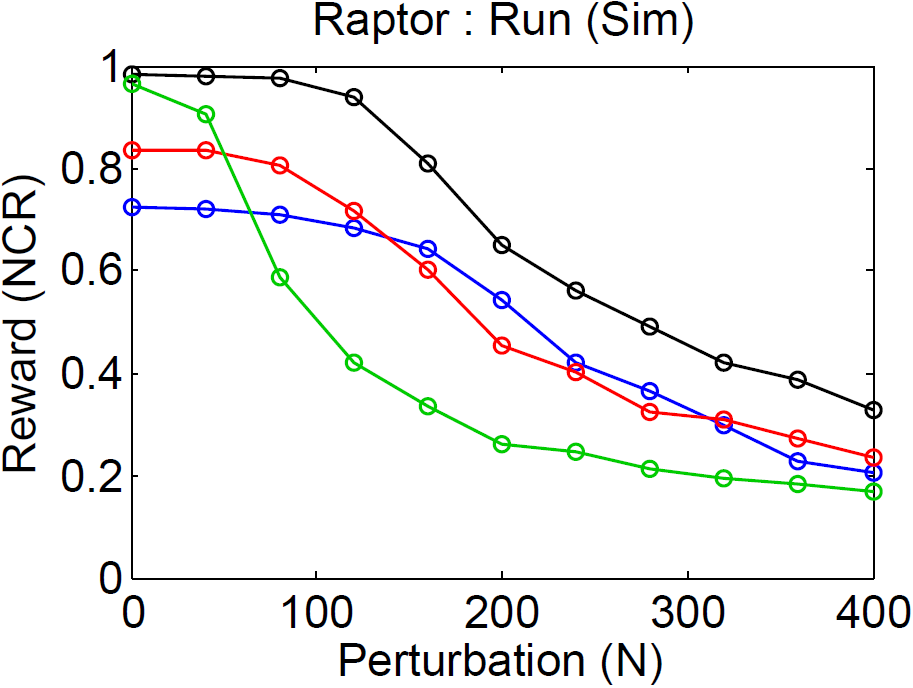
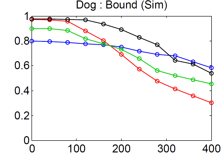
Policy Robustness: To evaluate robustness, we recorded the NCR achieved by each policy when subjected to external perturbations. The perturbations assume the form of random forces applied to the trunk of the characters. Figure 3 illustrates the performance of the policies when subjected to perturbations of different magnitudes. The magnitude of the forces are constant, but direction varies randomly. Each force is applied for 0.1 to 0.4s, with 1 to 4s between each perturbation. Performance is estimated using the average over 128 episodes of length 20s each. For the biped walk, the Tor policy is significantly less robust than those for the other types of actions, while the MTU policy is the least robust for the raptor run. Overall, the PD policies are among the most robust for all the motions. In addition to external forces, we also evaluate robustness over randomly generated terrain consisting of bumps with varying heights and slopes with varying steepness. We evaluate the performance on irregular terrain (Figure 10, supplemental material). There are few discernible patterns for this test. The Vel and MTU policies are significantly worse than the Tor and PD policies for the dog bound on the bumpy terrain. The unnatural jittery behavior of the dog Tor policy proves to be surprisingly robust for this scenario. We suspect that the behavior prevents the trunk from contacting the ground for extended periods for time, and thereby escaping our system’s fall detection.

Figure 3: Performance when subjected to random perturbation forces of different magnitudes.

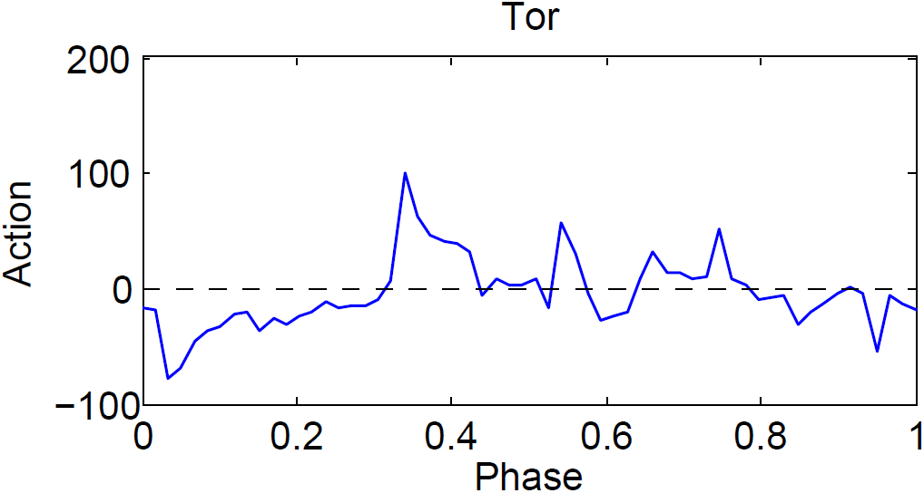
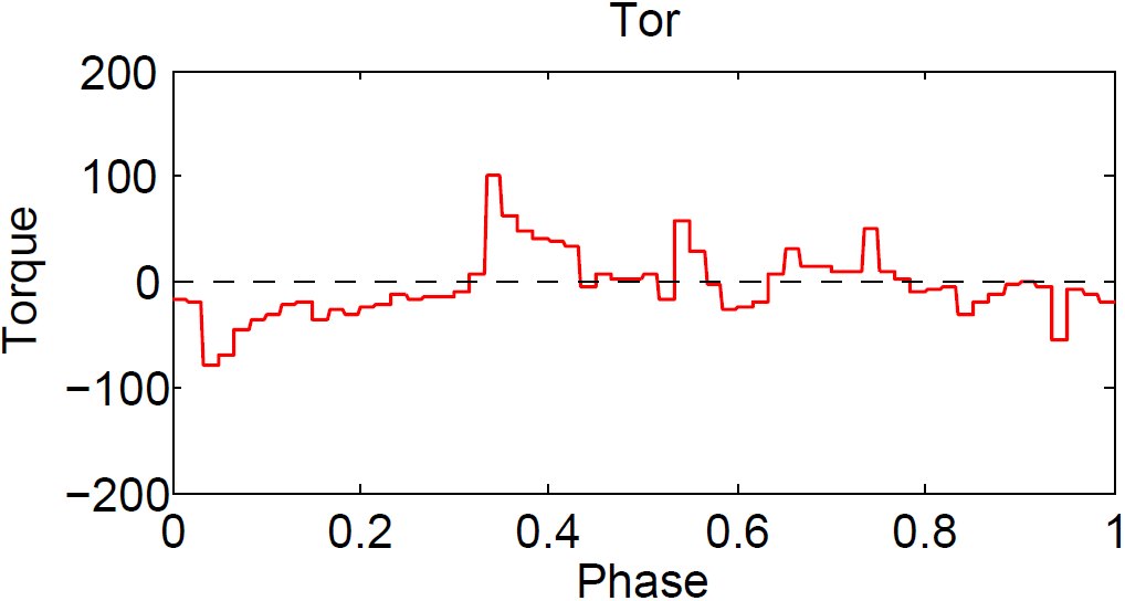
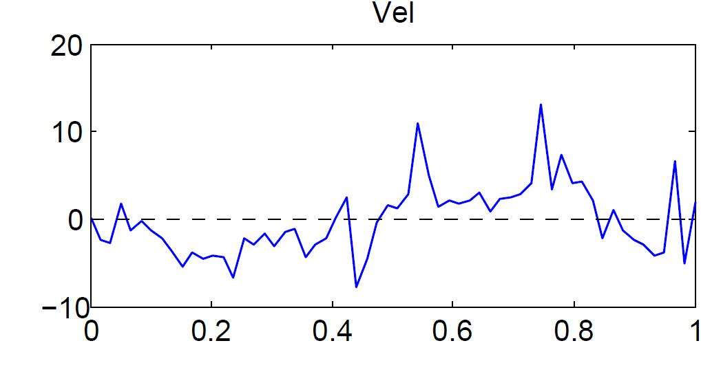
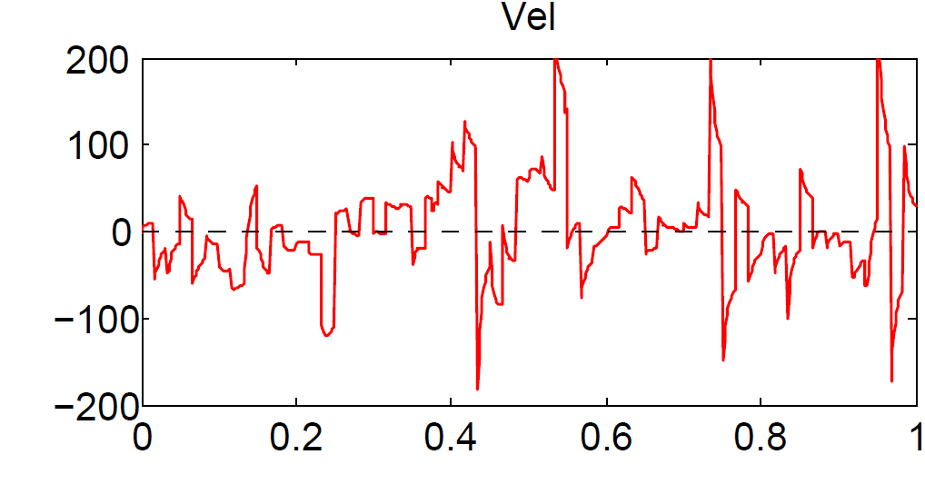
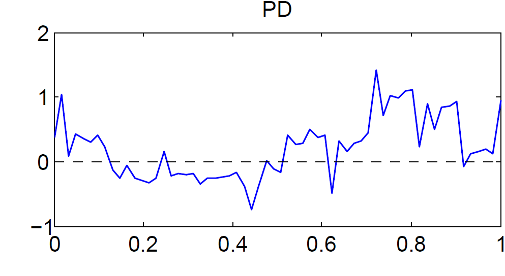
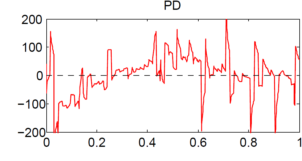
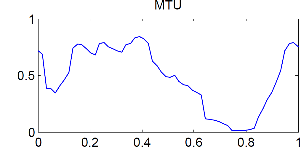
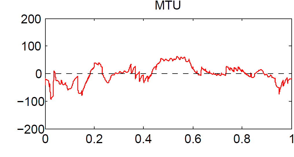
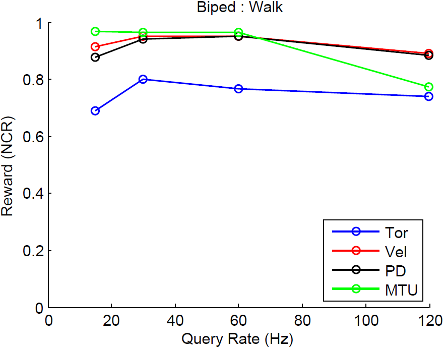
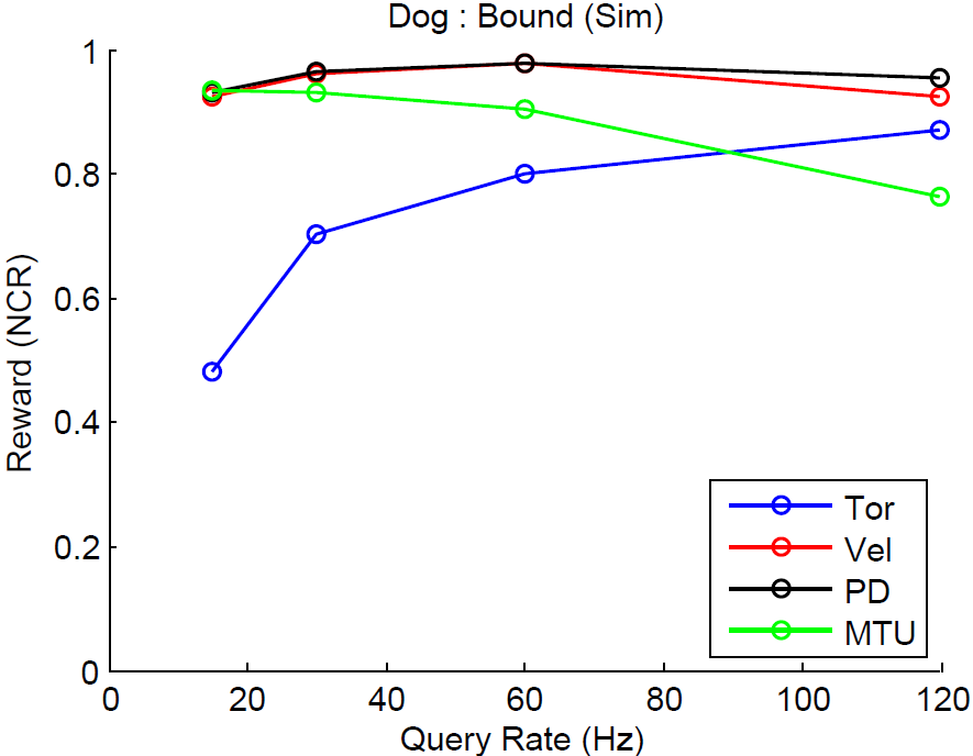
Query Rate: Figure 4 compares the performance of different parameterizations for different policy query rates. Separate policies are trained with queries of 15Hz, 30Hz, 60Hz, and 120Hz. Actuation models that incorporate low-level feedback such as PD and Vel, appear to cope more effectively to lower query rates, while the Tor degrades more rapidly at lower query rates. It is not yet obvious to us why MTU policies appear to perform better at lower query rates and worse at higher rates. Lastly, Figure 11 shows the policy outputs as a function of time for the four actuation models, for a particular joint, as well as showing the resulting joint torque. Interestingly, the MTU action is visibly smoother than the other actions and results in joint torques profiles that are smoother than those seen for PD and Vel.

Figure 4: Performance of policies with different query rates for the biped (left) and dog (right). Separate policies are trained for each query rate.

6 Related Work

DeepRL has driven impressive recent advances in learning motion control, i.e., solving for continuous-action control problems using reinforcement learning. All four of the actions types that we explore have seen previous use in the machine learning literature. WawrzyńSki & Tanwani (2013) use an actor-critic approach with experience replay to learn skills for an octopus arm (actuated by a simple muscle model) and a planar half cheetah (actuated by joint-based PD-controllers). Recent work on deterministic policy gradients (Lillicrap et al., 2015) and on RL benchmarks, e.g., OpenAI Gym, generally use joint torques as the action space, as do the test suites in recent work  (Schulman et al., 2015) on using generalized advantage estimation. Other recent work uses: the PR2 effort control interface as a proxy for torque control (Levine et al., 2015); joint velocities (Gu et al., 2016); velocities under an implicit control policy (Mordatch et al., 2015); or provide abstract actions (Hausknecht & Stone, 2015). Our learning procedures are based on prior work using actor-critic approaches with positive temporal difference updates (Van Hasselt, 2012).

Work in biomechanics has long recognized the embodied nature of the control problem and the view that musculotendon systems provide “preflexes” (Loeb, 1995) that effectively provide a form intelligence by mechanics (Blickhan et al., 2007), as well as allowing for energy storage. The control strategies for physics-based character simulations in computer animation also use all the forms of actuation that we evaluate in this paper. Representative examples include quadratic programs that solve for joint torques (de Lasa et al., 2010), joint velocities for skilled bicycle stunts (Tan et al., 2014), muscle models for locomotion (Wang et al., 2012; Geijtenbeek et al., 2013), mixed use of feed-forward torques and joint target angles (Coros et al., 2011), and joint target angles computed by learned linear (time-indexed) feedback strategies (Liu et al., 2016). Lastly, control methods in robotics use a mix of actuation types, including direct-drive torques (or their virtualized equivalents), series elastic actuators, PD control, and velocity control. These methods often rely heavily on model-based solutions and thus we do not describe these in further detail here.

7 Conclusions

Our experiments suggest that action parameterizations that include basic local feedback, such as PD target angles, MTU activations, or target velocities, can improve policy performance and learning speed across different motions and character morphologies. Such models more accurately reflect the embodied nature of control in biomechanical systems, and the role of mechanical components in shaping the overall dynamics of motions and their control. The difference between low-level and high-level action parameterizations grow with the complexity of the characters, with high-level parameterizations scaling more gracefully to complex characters.

Our results have only been demonstrated on planar articulated figure simulations; the extension to 3D currently remains as future work. Tuning actuator parameters for complex actuation models such as MTUs remains challenging. Though our actuator optimization technique is able to improve performance as compared to manual tuning, the resulting parameters may still not be optimal for the desired task. Therefore, our comparisons of MTUs to other action parameterizations may not be reflective of the full potential of MTUs with more optimal actuator parameters. Furthermore, our actuator optimization currently tunes parameters for a specific motion, rather than a larger suite of motions, as might be expected in nature.

To better understand the effects of different action parameterizations, we believe it will be beneficial to replicate our experiments with other reinforcement learning algorithms and motion control tasks. As is the case with other results in this area, hyperparameter choices can have a significant impact on performance, and therefore it is difficult to make definitive statements with regards to the merits of the various actions spaces that we have explored. However, we believe that the general trends we observed are likely to generalize.

Finally, it is reasonable to expect that evolutionary processes would result in the effective co-design of actuation mechanics and control capabilities. Developing optimization and learning algorithms to allow for this kind of co-design is a fascinating possibility for future work.

Supplementary Material

Algorithm 1 Actor-critic Learning Using Positive Temporal Differences

1:  $\theta\leftarrow$ random weights

2:  $\phi\leftarrow$ random weights

2:  

3:  while not done do

4:     for $step=1,...,m$ do

5:        $s\leftarrow$ start state

6:        $\lambda\leftarrow\mathrm{Ber}(\epsilon_{t})$

7:        $a\leftarrow\mu_{\theta}(s)+\lambda\mathcal{N}(0,\Sigma)$

8:        Apply $a$ and simulate forward 1 step

9:        $s^{\prime}\leftarrow$ end state

10:        $r\leftarrow$ reward

11:        $\tau\leftarrow(s,a,r,s^{\prime},\lambda)$

12:        store $\tau$ in replay memory

12:        

13:        if episode terminated then

14:           Sample $s_{0}$ from $p_{0}(s)$

15:           Reinitialize state $s$ to $s_{0}$

16:        end if

17:     end for

17:     

18:     Update critic:

19:     Sample minibatch of $n$ tuples $\{\tau_{i}=(s_{i},a_{i},r_{i},\lambda_{i},s_{i}^{\prime})\}$ from replay memory

20:     for each $\tau_{i}$ do

21:        $\delta_{i}\leftarrow r_{i}+\gamma V_{\phi}(s^{\prime}_{i})-V_{\phi}(s_{i})$

22:        $\phi\leftarrow\phi+\alpha_{V}\frac{1}{n}\delta_{i}\triangledown_{\phi}V_{\phi}(s_{i})$

23:     end for

23:     

24:     Update actor:

25:     Sample minibatch of $n$ tuples $\{\tau_{j}=(s_{j},a_{j},r_{j},\lambda_{j},s_{j}^{\prime})\}$ from replay memory where $\lambda_{j}=1$

26:     for each $\tau_{j}$ do

27:        $\delta_{j}\leftarrow r_{j}+\gamma V_{\phi}(s^{\prime}_{j})-V_{\phi}(s_{j})$

28:        if $\delta_{j}>0$ then

29:           $\triangledown a_{j}\leftarrow a_{j}-\mu_{\theta}(s_{j})$

30:           $\triangledown\tilde{a}_{j}\leftarrow\mathrm{BoundActionGradient}(\triangledown a_{j},\mu_{\theta}(s_{j}))$

31:           $\theta\leftarrow\theta+\alpha_{\pi}\frac{1}{n}\triangledown_{\theta}\mu_{\theta}(s_{j})\Sigma^{-1}\triangledown\tilde{a}_{j}$

32:        end if

33:     end for

34:  end while

Algorithm 2 Alternating Actuator Optimization

1:  $\theta\leftarrow\theta_{0}$

2:  $\psi\leftarrow\psi_{0}$

3:  while not done do

4:     $\theta\leftarrow\mathop{\mathrm{argmax}}_{\theta^{\prime}}J(\pi_{\theta^{\prime}},\psi)$ with Algorithm 1

5:     $\psi\leftarrow\mathop{\mathrm{argmax}}_{\psi^{\prime}}J(\pi_{\theta},\psi^{\prime})$ with CMA

6:  end while

MTU Actuator Optimization

The actuator parameters $\psi$ can be interpreted as a parameterization of the dynamics of the system $p(s^{\prime}|s,a,\psi)$. The expected cumulative reward can then be re-parameterized according to

$$J(\pi_{\theta},\psi)=\int_{\mathcal{S}}d_{\theta}(s|\psi)\int_{\mathcal{A}}\pi_{\theta}(s,a)A(s,a)da\ ds$$

where $d_{\theta}(s|\psi)=\int_{\mathcal{S}}\sum_{t=0}^{T}\gamma^{t}p_{0}(s_{0})p(s_{0}\rightarrow s|t,\pi_{\theta},\psi)ds_{0}$. $\theta$ and $\psi$ are then learned in tandem following Algorithm 2. This alternating method optimizes both the control and dynamics in order to maximize the expected value of the agent, as analogous to the role of evolution in biomechanics. During each pass, the policy parameters $\theta$ are trained to improve the agent’s expected value for a fixed set of actuator parameters $\psi$. Next, $\psi$ is optimized using CMA to improve performance while keeping $\theta$ fixed. The expected value of each CMA sample of $\psi$ is estimated using the average cumulative reward over multiple rollouts.

Figure 5 illustrates the improvement in performance during the optimization process, as applied to motions for three different agents. Figure 6 compares the learning curves for the initial and final MTU parameters, for the same three motions.

Figure 5: Performance of intermediate MTU policies and actuator parameters per pass of actuator optimization following Algorithm 2.

Figure 6: Learning curves comparing initial and optimized MTU parameters.

Bounded Action Space

Properties such as torque and neural activation limits result in bounds on the range of values that can be assumed by actions for a particular parameterization. Improper enforcement of these bounds can lead to unstable learning as the gradient information outside the bounds may not be reliable (Hausknecht & Stone, 2015). To ensure that all actions respect their bounds, we adopt a method similar to the inverting gradients approach proposed by Hausknecht & Stone (2015). Let $\triangledown a=(a-\mu(s))A(s,a)$ be the empirical action gradient from the policy gradient estimate of a Gaussian policy. Given the lower and upper bounds $[l^{i},u^{i}]$ of the $i$th action parameter, the bounded gradient of the $i$th action parameter $\triangledown\tilde{a}^{i}$ is determined according to

$$\triangledown\tilde{a}^{i}=\begin{cases}l^{i}-\mu^{i}(s),&\text{$\mu^{i}(s)<l^{i}$ and $\triangledown a^{i}<0$}\\ u^{i}-\mu^{i}(s),&\text{$\mu^{i}(s)>u^{i}$ and $\triangledown a^{i}>0$}\\ \triangledown a^{i},&\text{otherwise}\end{cases}$$

Unlike the inverting gradients approach, which scales all gradients depending on proximity to the bounds, this method preserves the empirical gradients when bounds are respected, and alters the gradients only when bounds are violated.

Reward

The terms of the reward function are defined as follows:

$$r_{pose}=\mathrm{exp}\left(-||q^{*}-q||^{2}_{W}\right),\qquad r_{vel}=\mathrm{exp}\left(-||\dot{q}^{*}-\dot{q}||^{2}_{W}\right)$$

$$r_{end}=\mathrm{exp}\left(-40\sum_{e}||x^{*}_{e}-x_{e}||^{2}\right)$$

$$r_{root}=\mathrm{exp}\left(-10(h^{*}_{root}-h_{root})^{2}\right),\qquad r_{com}=\mathrm{exp}\left(-10||\dot{x}^{*}_{com}-\dot{x}_{com}||^{2}\right)$$

$q$ and $q^{*}$ denotes the character pose and reference pose represented in reduced-coordinates, while $\dot{q}$ and $\dot{q}^{*}$ are the respective joints velocities. $W$ is a manually-specified per joint diagonal weighting matrix. $h_{root}$ is the height of the root from the ground, and $\dot{x}_{com}$ is the center of mass velocity.

Figure 7: Left: fixed initial state biases agent to regions of the state space near the initial state, particular during early iterations of training. Right: initial states sampled from reference trajectory allows agent to explore state space more uniformly around reference trajectory.

Figure 8: Neural Network Architecture. Each policy is represented by a three layered network, with 512 and 256 fully-connected hidden units, followed by a linear output layer.

Parameter	Value	Description
$\gamma$	0.9	cumulative reward discount factor
$\alpha_{\pi}$	0.001	actor learning rate
$\alpha_{V}$	0.01	critic learning rate
momentum	0.9	stochastic gradient descent momentum
$\phi$ weight decay	0	L2 regularizer for critic parameters
$\theta$ weight decay	0.0005	L2 regularizer for actor parameters
minibatch size	32	tuples per stochastic gradient descent step
replay memory size	500000	number of the most recent tuples stored for future updates

Table 2: Training hyperparameters.

Character + Actuation Model	State Parameters	Action Parameters	Actuator Parameters
Biped + Tor	58	6	0
Biped + Vel	58	6	6
Biped + PD	58	6	12
Biped + MTU	74	16	114
Raptor + Tor	154	18	0
Raptor + Vel	154	18	18
Raptor + PD	154	18	36
Raptor + MTU	194	40	258
Dog + Tor	170	20	0
Dog + Vel	170	20	20
Dog + PD	170	20	40
Dog + MTU	214	44	282

Table 3: The number of state, action, and actuation model parameters for different characters and actuation models.

Character + Actuation	Motion	Performance (NCR)	Learning Speed (AUC)
Biped + Tor	Walk	0.7662 $\pm$ 0.3117	0.4788
Biped + Vel	Walk	0.9520 $\pm$ 0.0034	0.6308
Biped + PD	Walk	0.9524 $\pm$ 0.0034	0.6997
Biped + MTU	Walk	0.9584 $\pm$ 0.0065	0.7165
Biped + Tor	March	0.9353 $\pm$ 0.0072	0.7478
Biped + Vel	March	0.9784 $\pm$ 0.0018	0.9035
Biped + PD	March	0.9767 $\pm$ 0.0068	0.9136
Biped + MTU	March	0.9484 $\pm$ 0.0021	0.5587
Biped + Tor	Run	0.9032 $\pm$ 0.0102	0.6938
Biped + Vel	Run	0.9070 $\pm$ 0.0106	0.7301
Biped + PD	Run	0.9057 $\pm$ 0.0056	0.7880
Biped + MTU	Run	0.8988 $\pm$ 0.0094	0.5360
Raptor + Tor	Run (Sim)	0.7265 $\pm$ 0.0037	0.5061
Raptor + Vel	Run (Sim)	0.9612 $\pm$ 0.0055	0.8118
Raptor + PD	Run (Sim)	0.9863 $\pm$ 0.0017	0.9282
Raptor + MTU	Run (Sim)	0.9708 $\pm$ 0.0023	0.6330
Raptor + Tor	Run	0.6141 $\pm$ 0.0091	0.3814
Raptor + Vel	Run	0.8732 $\pm$ 0.0037	0.7008
Raptor + PD	Run	0.9548 $\pm$ 0.0010	0.8372
Raptor + MTU	Run	0.9533 $\pm$ 0.0015	0.7258
Dog + Tor	Bound (Sim)	0.8016 $\pm$ 0.0034	0.5472
Dog + Vel	Bound (Sim)	0.9788 $\pm$ 0.0044	0.7862
Dog + PD	Bound (Sim)	0.9797 $\pm$ 0.0012	0.9280
Dog + MTU	Bound (Sim)	0.9033 $\pm$ 0.0029	0.6825
Dog + Tor	Rear-Up	0.8151 $\pm$ 0.0113	0.5550
Dog + Vel	Rear-Up	0.7364 $\pm$ 0.2707	0.7454
Dog + PD	Rear-Up	0.9565 $\pm$ 0.0058	0.8701
Dog + MTU	Rear-Up	0.8744 $\pm$ 0.2566	0.7932

Table 4: Performance of policies trained for the various characters and actuation models. Performance is measured using the normalized cumulative reward (NCR) and learning speed is represented by the normalized area under each learning curve (AUC). The best performing parameterizations for each character and motion are in bold.

Figure 9: Simulated Motions Using the PD Action Representation. The top row uses an MTU action space while the remainder are driven by a PD action space.

Figure 10: Performance of different action parameterizations when traveling across randomly generated irregular terrain. (left) Dog running across bumpy terrain, where the height of each bump varies uniformly between 0 and a specified maximum height. (middle) and (right) biped and dog traveling across randomly generated slopes with bounded maximum steepness.

Figure 11: Policy actions over time and the resulting torques for the four action types. Data is from one biped walk cycle (1s). Left: Actions (60 Hz), for the right hip for PD, Vel, and Tor, and the right gluteal muscle for MTU. Right: Torques applied to the right hip joint, sampled at 600 Hz.

Figure 12: Learning curves for different state representations including state + target state, state + phase, and only state.

References

- Blickhan et al. (2007) Reinhard Blickhan, Andre Seyfarth, Hartmut Geyer, Sten Grimmer, Heiko Wagner, and Michael Günther. Intelligence by mechanics. Philosophical Transactions of the Royal Society of London A: Mathematical, Physical and Engineering Sciences, 365(1850):199–220, 2007.
- Coros et al. (2011) Stelian Coros, Andrej Karpathy, Ben Jones, Lionel Reveret, and Michiel van de Panne. Locomotion skills for simulated quadrupeds. ACM Transactions on Graphics, 30(4):Article TBD, 2011.
- de Lasa et al. (2010) Martin de Lasa, Igor Mordatch, and Aaron Hertzmann. Feature-based locomotion controllers. In ACM Transactions on Graphics (TOG), volume 29, pp. 131. ACM, 2010.
- Geijtenbeek et al. (2013) Thomas Geijtenbeek, Michiel van de Panne, and A. Frank van der Stappen. Flexible muscle-based locomotion for bipedal creatures. ACM Transactions on Graphics, 32(6), 2013.
- Geyer et al. (2003) Hartmut Geyer, Andre Seyfarth, and Reinhard Blickhan. Positive force feedback in bouncing gaits? Proc. Royal Society of London B: Biological Sciences, 270(1529):2173–2183, 2003.
- Gu et al. (2016) Shixiang Gu, Ethan Holly, Timothy Lillicrap, and Sergey Levine. Deep reinforcement learning for robotic manipulation. arXiv preprint arXiv:1610.00633, 2016.
- Hausknecht & Stone (2015) Matthew J. Hausknecht and Peter Stone. Deep reinforcement learning in parameterized action space. CoRR, abs/1511.04143, 2015.
- Konda & Tsitsiklis (2000) Vijay Konda and John Tsitsiklis. Actor-critic algorithms. In SIAM Journal on Control and Optimization, pp. 1008–1014. MIT Press, 2000.
- Levine et al. (2015) Sergey Levine, Chelsea Finn, Trevor Darrell, and Pieter Abbeel. End-to-end training of deep visuomotor policies. CoRR, abs/1504.00702, 2015.
- Lillicrap et al. (2015) Timothy P. Lillicrap, Jonathan J. Hunt, Alexander Pritzel, Nicolas Heess, Tom Erez, Yuval Tassa, David Silver, and Daan Wierstra. Continuous control with deep reinforcement learning. CoRR, abs/1509.02971, 2015.
- Liu et al. (2016) Libin Liu, Michiel van de Panne, and KangKang Yin. Guided learning of control graphs for physics-based characters. ACM Transactions on Graphics, 35(3), 2016.
- Loeb (1995) GE Loeb. Control implications of musculoskeletal mechanics. In Engineering in Medicine and Biology Society, 1995., IEEE 17th Annual Conference, volume 2, pp. 1393–1394. IEEE, 1995.
- Mordatch et al. (2015) Igor Mordatch, Kendall Lowrey, Galen Andrew, Zoran Popovic, and Emanuel Todorov. Interactive control of diverse complex characters with neural networks. In Advances in Neural Information Processing Systems 28, pp. 3132–3140, 2015.
- Schulman et al. (2015) John Schulman, Philipp Moritz, Sergey Levine, Michael I. Jordan, and Pieter Abbeel. High-dimensional continuous control using generalized advantage estimation. CoRR, abs/1506.02438, 2015.
- Silver et al. (2014) David Silver, Guy Lever, Nicolas Heess, Thomas Degris, Daan Wierstra, and Martin Riedmiller. Deterministic policy gradient algorithms. In Proc. International Conference on Machine Learning, pp. 387–395, 2014.
- Sutton et al. (2001) R. Sutton, D. Mcallester, S. Singh, and Y. Mansour. Policy gradient methods for reinforcement learning with function approximation, 2001.
- Tan et al. (2014) Jie Tan, Yuting Gu, C. Karen Liu, and Greg Turk. Learning bicycle stunts. ACM Trans. Graph., 33(4):50:1–50:12, 2014. ISSN 0730-0301.
- Van Hasselt (2012) Hado Van Hasselt. Reinforcement learning in continuous state and action spaces. In Reinforcement Learning, pp. 207–251. Springer, 2012.
- Wang et al. (2012) Jack M. Wang, Samuel R. Hamner, Scott L. Delp, Vladlen Koltun, and More Specifically. Optimizing locomotion controllers using biologically-based actuators and objectives. ACM Trans. Graph, 2012.
- WawrzyńSki & Tanwani (2013) Paweł WawrzyńSki and Ajay Kumar Tanwani. Autonomous reinforcement learning with experience replay. Neural Networks, 41:156–167, 2013.