A Deep Convolutional Neural Network using Directional Wavelets for Low-dose X-ray CT Reconstruction

Abstract

Purpose: Due to the potential risk of inducing cancer, radiation exposure by X-ray CT devices should be reduced for routine patient scanning. However, in low-dose X-ray CT, severe artifacts typically occur due to photon starvation, beam hardening, and other causes, all of which decrease the reliability of the diagnosis. Thus, a high-quality reconstruction method from low-dose X-ray CT data has become a major research topic in the CT community. Conventional model-based de-noising approaches are, however, computationally very expensive, and image-domain de-noising approaches cannot readily remove CT-specific noise patterns. To tackle these problems, we want to develop a new low-dose X-ray CT algorithm based on a deep-learning approach.

Method: We propose an algorithm which uses a deep convolutional neural network (CNN) which is applied to the wavelet transform coefficients of low-dose CT images. More specifically, using a directional wavelet transform to extract the directional component of artifacts and exploit the intra- and inter- band correlations, our deep network can effectively suppress CT-specific noise. In addition, our CNN is designed with a residual learning architecture for faster network training and better performance.

Results: Experimental results confirm that the proposed algorithm effectively removes complex noise patterns from CT images derived from a reduced X-ray dose. In addition, we show that the wavelet-domain CNN is efficient when used to remove noise from low-dose CT compared to existing approaches. Our results were rigorously evaluated by several radiologists at the Mayo Clinic and won second place at the 2016 “Low-Dose CT Grand Challenge.”

Conclusions: To the best of our knowledge, this work is the first deep-learning architecture for low-dose CT reconstruction which has been rigorously evaluated and proven to be effective. In addition, the proposed algorithm, in contrast to existing model-based iterative reconstruction (MBIR) methods, has considerable potential to benefit from large data sets. Therefore, we believe that the proposed algorithm opens a new direction in the area of low-dose CT research.

I Introduction

X-ray computed tomography (CT) is a commonly used medical imaging method capable of showing fine details inside the human body, such as structures of the lung and bones. However, CT is inherently associated with a much higher X-ray dose compared to simple film radiography. Due to the strong evidence of radiation-related cancer Brenner and Hall (2007), the recent research interest in CT has mainly focused on minimizing the X-ray dose to reduce the risk to patients Yu et al. (2009). One popular technique by which to do so is to reduce the number of X-ray photons emitted from the X-ray source by controlling the currents applied to the X-ray tube. However, such a technique typically results in reduced image quality due to the low signal-to-noise ratio (SNR) measurements. Accordingly, the success of low-dose CT is strongly determined by the de-noising technique used.

There are various image de-noising approaches. Popular approaches include total variation minimization Chambolle (2004) and wavelet shrinkage approaches Portilla et al. (2003); Crouse, Nowak, and Baraniuk (1998). More recent methods use non-local statistics or the degree of self-similarity of the images Dabov et al. (2007); Kim et al. (2015). However, one of the limitations of existing image-domain de-noising approaches is that they are not ideal when used with CT-specific noise patterns, as complicated streaking artifacts usually occur in low-dose CT due to photon starvation and beam hardening Hsieh (2003). In addition, CT data are subject to sophisticated non-linear acquisition processes, which lead to non-stationary and non-Gaussian noise processes. To address these limitations, model-based iterative reconstruction (MBIR) was developed. It relies on the physical modelling of projection/backprojection operators and the statistical modelling of the noise in projection measurements Beister, Kolditz, and Kalender (2012).

Researchers of MBIR algorithms have developed optimization techniques to speed up the convergence of MBIRRamani and Fessler (2012); Kim, Ramani, and Fessler (2015) as well as new regularization terms that can reduce the noise and preserve the edge detailsXu et al. (2012); Wieczorek et al. (2015); Zhang et al. (2015); Cho and Fessler (2015). Although the existing MBIR approaches may include a system geometry model that takes the CT scanner geometry and physical effects into account, MBIR approaches typically perform computationally expensive iterative projection/backprojection steps. In addition, it is difficult for MBIR to use the rich information available in large-scale CT data sets, as only a few parameters can be trained in typical MBIR algorithms.

In computer vision applications, de-noising algorithms using an artificial neural network have been intensively studied and have shown impressive performance capabilities Zhang and Salari (2005); Jain and Seung (2009); Nasri and Nezamabadi-pour (2009); Vincent et al. (2010); Burger, Schuler, and Harmeling (2012); Xie, Xu, and Chen (2012); Mao, Shen, and Yang (2016); Chen, Yu, and Pock (2015). In this de-noising framework, the parameters of a neural network are trained by supervised learning using large training data sets and the trained network is then applied to remove noise from the test data set. Although classical neural network approaches were limited to shallow structures due to gradient vanishing/exploding or overfitting problems, the recent development of new network units, such as the rectified linear unit(ReLU), max pooling, dropout and batch normalization, mitigate the problems associated with classical methods, leaving much deeper networks with more power. For the last few years, researchers have had great successes from deep networks in many low-level computer vision applications, such as de-noising Xie, Xu, and Chen (2012); Mao, Shen, and Yang (2016); Chen, Yu, and Pock (2015) and super-resolution applications Dong et al. (2014); Kim, Kwon Lee, and Mu Lee (2016).

Inspired by the success of the deep convolutional neural network, we propose a novel low-dose CT de-noising framework designed to detect and remove CT-specific noise patterns. Specifically, instead of using the publicly available image-domain CNN architecture, we propose a new CNN architecture optimized for CT de-noising. In particular, based on the observation that a directional wavelet transform can detect the directional components of noise, we construct a deep CNN network in the wavelet domain. More specifically, the network is trained with wavelet coefficients from the CT images after applying the contourlet transformZhou, Cunha, and Do (2005). To achieve the best performance, the proposed wavelet-domain network consists of operation units such as convolution, batch normalizationIoffe and Szegedy (2015); Ioffe (2017), and rectifier linear unit (ReLU) Nair and Hinton (2010) with residual learningHe et al. (2016) using various types of bypass connections.

The performance of the proposed de-noising framework was rigorously evaluated using the data set of the 2016 Low-Dose CT Grand Challenge McCollough (2016) and showed significant improvements compared to conventional de-noising approaches. Extensive experimental results also confirmed the effectiveness of the proposed network architecture.

Figure 1: Various noise patterns in low-dose CT images: (a) Gaussian noise, and (b) streaking artifacts

II Background

II.1 Low-dose X-ray CT Physics

The statistics of X-ray measurements are often described by a Poisson distribution. Specifically, a Poisson model for the intensity measurement is

$$I_{i}\sim Poisson\left\{b_{i}e^{-[{\mathbf{A}}{\mathbf{x}}]_{i}}+r_{i}\right\},\quad i=1,\cdots,N_{m},$$ (1)

where ${\mathbf{A}}$ is a system matrix (projection operator), ${\mathbf{x}}=(x_{1},\cdots,x_{N_{v}})\in{\mathbb{R}}^{N_{v}}_{+}$ is a vector for the representation of attenuation coefficients with units of inverse length, $N_{m}$ is the number of measurements, $N_{v}$ is the number of image voxels, $b_{i}$ denotes the X-ray source intensity of the $i$th ray, and $r_{i}$ denotes the background contributions of scatter and electrical noise. After taking the log, the sinogram data is often approximated as a weighted Gaussian:

$$y_{i}\sim N\left([{\mathbf{A}}{\mathbf{x}}]_{i},\dfrac{\bar{I}_{i}}{(\bar{I}_{i}-r_{i})^{2}}\right),$$ (2)

where $\bar{I}_{i}=E[I_{i}]$.

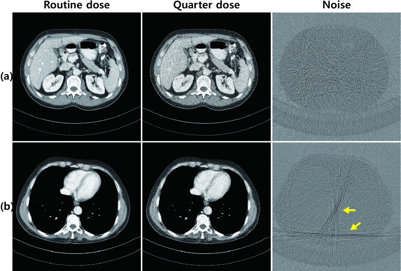
In practice, polychromatic X-ray can produce various artifacts such as beam-hardening. Given that the lower energy X-ray photons are seldom measured by detectors, the linearity of the projection data and attenuation coefficients is no longer valid. In addition to these beam-hardening related artifacts, there are photon-starvation artifacts because bones have higher attenuation and thus absorb a considerable amount of X-ray photons. Specifically, ribs and backbone are located on opposite sides of the body; therefore, an X-ray beam should pass through more than two bones depending on the direction of the X-ray path such that we lose information about the tissues between these bones. This results in streaking artifacts in these directions (see Fig. 1).

II.2 Conventional algorithms for low-dose X-ray CT

II.2.1 Image domain de-noising

One of the simplest approaches to low-dose X-ray CT is image-domain de-noising. Among various approaches, wavelet shrinkage approaches which decompose an image into low- and high-frequency components with thresholding for the high-frequency coefficients have been widely used Portilla et al. (2003). Advanced algorithms in this field exploit the intra- and inter- correlations of the wavelet coefficients of image details by statistical modeling Crouse, Nowak, and Baraniuk (1998). Wavelet shrinkage approaches indeed correspond to the application of a sparsity penalty for wavelet transform coefficients. Accordingly, sparsity-driven de-noising algorithms have been extensively studied, with the approach known as total variation (TV) widely used Chambolle (2004). Unfortunately, this approach often produces cartoon-like artifacts.

To solve this problem, some studies approximate noisy patches using a sparse linear combination of the elements of a learned dictionaryElad and Aharon (2006). Newer approaches use the non-local statistics of images based on the observation that different local patches in the same image are often similar in appearance. For example, block matching with a 3D collaborative filtering algorithm (BM3D) Dabov et al. (2007) uses the self-similarity of small patches and applies group-based filtering to similar patches to suppress noise. However, these methods have not been designed directly for X-ray CT artifacts. Therefore, it is often not possible to detect and remove CT-specific noise features.

II.2.2 MBIR for low-dose X-ray CT

To address these issues, model-based iterative reconstruction (MBIR) approaches have been studied extensively. Specifically, using the model in Eq. (2), this problem is formulated as the following minimization problem:

$$\min_{{\mathbf{x}}}\left\{\dfrac{1}{2}\|{\mathbf{y}}-{\mathbf{A}}{\mathbf{x}}\|^{2}_{w}+\lambda R({\mathbf{x}})\right\},$$ (3)

where $\|{\mathbf{y}}-{\mathbf{A}}{\mathbf{x}}\|^{2}_{w}$ is a data fidelity term weighted by $\bar{I}_{i}/(\bar{I}_{i}-r_{i})$, $R({\mathbf{x}})$ is a regularization term (penalty term) that imposes additional requirements such as smoothness or sparsity, and $\lambda$ is a regularization parameter.

A popular regularization term is again total variation (TV) Chambolle (2004) regularization, based on the assumption that an image under gradient operation is sparse. Many researchers have developed different types of dictionary or non-local means methods. For example, a dictionary that represents image features such as edges is constructed or updated during the reconstruction processXu et al. (2012). In addition, existing ridgelets, shearlets, and curvelets can compose the dictionary Wieczorek et al. (2015). Other methods based on non-local means regularization have also been developed Zhang et al. (2015); Cho and Fessler (2015). Although there have been extensive studies to speed up convergenceRamani and Fessler (2012); Kim, Ramani, and Fessler (2015), these iterative reconstruction methods are on the other hand associated with high computational complexity of the projection/backprojection operators and iterative optimization steps for non-differentiable sparsity promoting penalties.

II.3 Convolutional neural networks

Dramatic improvements in parallel computing techniques allow the processing of large amounts of data for deep neural networks. The recent breakthroughs in deep neural networks originated from deep convolutional neural networks (CNNs) such as AlexNet Krizhevsky, Sutskever, and Hinton (2012). The convolutional neural network, inspired by the neural network of the visual cortex in animals, is a special case of an artificial neural network. Similar to typical neural networks, it consists of successive linear and non-linear functions, but the linear parts are specifically expressed by convolution operations. In particular, the local property of the convolution is known to be efficient with regard to understanding visual data, and the induced nonlinearity allows for far more complex data representations. The deeper the network becomes, the greater the abstraction of images.

The simplest form of the CNN output $y$ is expressed as

$$y=F(\Theta,x)=f_{n}(W_{n}f_{n-1}(\cdots(f_{2}(W_{2}f_{1}(W_{1}x+b_{1})+b_{2})\cdots)+b_{n}),$$ (4)

where $x$ is the input, $y$ is the output, $W_{i}$ is the convolution matrix of the $i$-th layer, $b_{i}$ is the bias of the $i$-th convolution layer, $f_{i}$ is a nonlinear function, and $\Theta$ is the set of all tunable parameters including $W_{i}$ and $b_{i}$. Although there are several non-linearity functions, the rectified linear unit (ReLU)Nair and Hinton (2010), i.e., $f(x)=\max(x,0)$, is commonly used in modern deep architectures. The goal of the CNN framework is then to find an optimal parameter set $\Theta$ with $K$ inputs to minimize the empirical loss:

$$\sum_{k=1}^{K}L\left(y_{k},F(\Theta,x_{k})\right).$$ (5)

In this equation, $x_{k}$ and $y_{k}$ denote the $k$-th input and output, respectively. Here, $L$ typically denotes the cross-entropy loss in classification problems or the Euclidean distance in regression problems such as image de-noising. Assuming that all nonlinear functions and the loss functions are differentiable, the minimization problem or network training in (5) can be addressed by an error back-propagation method Cotter et al. (2011). In general, the performance of the deep network is determined by the network architecture and methods that overcome the overfitting problem.

For the last few years, various types of deep CNNs have been developed. Several key components of a recent deep CNN include batch normalization Ioffe and Szegedy (2015), bypass connection Kim, Kwon Lee, and Mu Lee (2016), and a contracting path Ronneberger, Fischer, and Brox (2015). These were developed to efficiently train the CNN and improve its performance capabilities. For example, the authors of one study Ioffe and Szegedy (2015) found that the change in the distribution of network activations, called the internal covariate shift, was one of the main culprits of a slow training rate. Thus, reducing the internal covariate shift improves the training and minimizes the data overfitting problem as a by-product. More specifically, the training data set is subdivided into basic data units designated as minibatches, and batch normalization is then performed as follows,

$$\begin{array}[]{ll}\mu_{\textit{B}}=\dfrac{1}{m}\Sigma^{m}_{i=1}x_{i}&\quad\quad\mbox{:batch mean}\\ \sigma^{2}_{\textit{B}}=\dfrac{1}{m}\Sigma^{m}_{i=1}(x_{i}-\mu_{\textit{B}})^{2}&\quad\quad\mbox{:batch variance}\\ \hat{x}_{i}=\dfrac{x_{i}-\mu_{\textit{B}}}{\sqrt{\sigma^{2}_{\textit{B}}+\epsilon}}&\quad\quad\mbox{:normalize}\\ y_{i}\leftarrow\gamma\hat{x}_{i}+\beta\equiv\textit{BN}_{\gamma,\beta}(x_{i})&\quad\quad\mbox{:scale and shift}\end{array}$$ (6)

where $m$ denotes the batch size, and $\gamma$ and $\beta$ are learnable parameters. A layer of CNN including batch normalization can then be represented by

$$y=f(BN(Wx)),$$ (7)

where $BN$ denotes batch normalization. The structure of the basic unit of the network is described in Fig. 2(b).

Figure 2: Basic unit of a deep CNN: (a) convolution layer and non-linearity (ReLU) layer, and (b) convolution layer, batch normalization (BN) layer and non-linearity (ReLU) layer

Figure 3: (a) Bypass connection as indicated by the black arrow, and (b) contracting path in a U-net as indicated by the red arrow

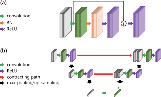
As a network becomes deeper, training of the network becomes more difficult, as the gradients are likely to disappear during an error back-propagation. To address this issue, the residual learning He et al. (2016) was developed, in which a bypass connection Kim, Kwon Lee, and Mu Lee (2016); Mao, Shen, and Yang (2016) and a contracting path Ronneberger, Fischer, and Brox (2015) were added to the network. More specifically, the features processed by bypass connections shown in Fig. 3(a) carry more image details, which helps to recover a better image and to secure advantages when back-propagating the gradient. Similarly, the contract path described in Fig. 3(b), originally introduced in U-net Ronneberger, Fischer, and Brox (2015) for image segmentation, preserves the details of high-resolution features. More specifically, a typical CNN has max-pooling (down-sampling) layers such that the information can be lost after passing these layers. To reduce this phenomenon, high-resolution features from the contracting path are combined with up-sampled output to provide the details of the high-resolution features.

A new CNN architecture was also introduced in which low-frequency image is passed on to the output and learning is performed only for residuals He et al. (2016). In terms of training, an adjustable gradient clipping method has been proposed to enable higher learning rates. It effectively speeds up the convergence for the training procedure. For the maximum convergence rate, the gradients are truncated to $\left[\frac{-\theta}{\gamma},\frac{\theta}{\gamma}\right]$, where $\gamma$ is the learning rate.

In the field of medical imaging, CNNs have been used exclusively for medical image analysis and computer-aided diagnosis Suzuki (2012). To the best of our knowledge, the proposed method is the first attempt to reduce the noise in low-dose CT images using a CNN. The details of our method are described in Section III.

III Method

The proposed network was motivated by the following observations: 1) a directional wavelet transform such as a contourlet (Zhou, Cunha, and Do, 2005) can efficiently decompose the directional components of noise to facilitate easier training of a deep network; and 2) low-dose CT images have complex noise, and a CNN has great potential to remove such noise; and 3) a deep neural network is ideal to capture various types of information from a large amount of training data.

III.1 Contourlet transform

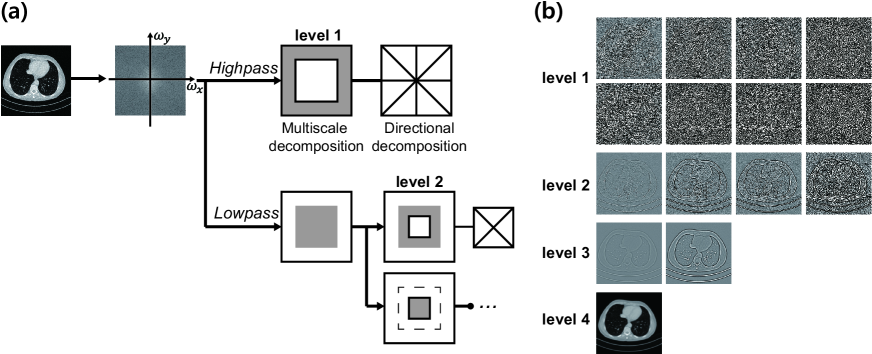
The contourlet transform consists of multiscale decomposition and directional decomposition. The non-subsampled contourlet transform is a shift-invariant version of the contourlet transform which consists of non-subsampled pyramids and non-subsampled directional filter banks, as shown in Fig. 4(a) (Zhou, Cunha, and Do, 2005). This filter bank does not have down-sampling or up-sampling and is therefore shift-invariant. Specifically, for a given a high-pass filter $H_{1}(z)$ and low-pass filter $H_{0}(z)$, non-subsampled pyramids are constructed by iteration of the filter banks. More specifically, the $k$th level pyramid is expressed by

$$H^{eq}_{n}(z)=\left\{\begin{array}[]{l l}H_{1}(z^{2^{n-1}})\Pi^{n-2}_{j=0}H_{0}(z^{2^{j}}),&\quad 1\leq n<2^{k}\\ \Pi^{n-1}_{j=0}H_{0}(z^{2^{j}}),&\quad n=2^{k}\end{array}\right.$$ (8)

Directional filter banks are then applied to the high-pass subbands to divide them into several directional components.

The scheme of the contourlet transform and several examples are described in Fig. 4. Here, each subband is shown with the same intensity range. Levels 1, 2, and 3 have high-frequency components of a low-dose CT image, such as edge information and noise. Note that the streaking noise between the bones is shown in the high-frequency bands.

Figure 4: Non-subsampled contourlet transform: (a) Scheme of contourlet transform. First, the image is split into high-pass and low-pass subbands. Then, non-subsampled directional filter banks divide the high-pass subband into directional subbands. This process is repeated in the low-pass subband. (b) Examples of the non-subsampled contourlet transform of a low-dose CT image. There are four levels, one each with eight, four, two, and one directional subbands.

III.2 Network architecture

Accordingly, in contrast to the conventional CNN-based denoiser Mao, Shen, and Yang (2016); Chen, Yu, and Pock (2015), our deep network was designed as a de-noising approach for wavelet coefficients, as shown in Fig. 5. This idea is closely related to classical de-noising approaches using wavelet shrinkage Donoho (1995), but instead of directly applying a closed-form shrinkage operator, the inter- and intra- scale correlations are exploited using a trainable shrinkage operator that transforms noisy wavelet coefficients into clean ones.

Figure 5: Proposed deep convolutional neural network architecture for wavelet domain de-noising

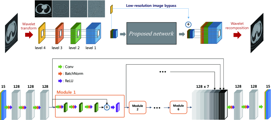
More specifically, as shown in Fig. 5, an input noisy image is initially decomposed into four decomposition levels using a contourlet transform Zhou, Cunha, and Do (2005) with a total of 15 channels (8, 4, 2, and 1 for levels 1, 2, 3 and 4, respectively) being generated. Given that undecimated multi-level contourlet transform is spatially invariant, the noisy wavelet coefficients can be processed in a patch-by-patch manner using a convolution operator. Here, each patch consists of 55$\times$55 square regions from 15 channels, resulting in the total size of 55$\times$55$\times$15. Patch-based image denoising techniques commonly use a $50\times 50$ patch, which is capable of describing the noise distribution and containing image information. We compared the performance of our network with a patch size between 40 and 60. The peak signal-to-noise ratio (PSNR) value of reconstruction images which definition is provided in the Sec. III.5 and the reconstruction time guided the proper patch size, i.e., 55.

In order to make the training more effective, our network takes full advantage of residual learning He et al. (2016). First, the low-frequency wavelet coefficients were bypassed and later added with the denoised wavelet coefficients, which significantly reduced the unnecessary load on the network. Because low-frequency images from low-dose image and routine-dose images are nearly equal, learning is not necessary during the training step. Furthermore, there are other types of internal bypass connections of the network, as shown in Fig. 5. These internal/external bypass connections help overcome the difficulty of training the deep network, resulting in better de-noising performance.

In particular, the proposed network contains 24 convolution layers, followed by a batch normalization layer and a ReLU layer for each convolution layer except the last one. Then, 128 sets of 3$\times$3$\times$15 convolution filters are used on the first layer to create 55$\times$55$\times$128 channels, after which 128 sets of 3$\times$3$\times$128 convolution filters are used in the subsequent layers. Our network consists of six modules, with each module consisting of a bypass connection and three convolution layers. In addition, our network has a channel concatenation layer Ronneberger, Fischer, and Brox (2015) which stacks the inputs of each module in the channel dimension. This allows the gradients to be back-propagated over a variety of paths, enabling faster end-to-end training.

III.3 Network training

Network training was performed by minimizing the loss function (5) with an additional $l_{2}$ regularization term for the network parameters. The regularization parameter $\lambda$ varies in the range of $[10^{-5},10^{-3}]$, and the performance of the proposed network was not sensitive to the choice of $\lambda$. In fact, our network showed similar performance regardless of $\lambda$ when it varied in the range of $[10^{-5},10^{-3}]$.

Minimization of the cost function was performed by means of conventional error back-propagation with the mini-batch stochastic gradient descent (SGD) Rumelhart, Hinton, and Williams (1986); Zhang (2004); Cotter et al. (2011) and the gradient clipping method. The convolution kernel weights were initialized using random Gaussian distributions. In the SGD, the initial learning rate ($\gamma$) equal to the gradient step size was set to $0.01$, and it continuously decreased to $10^{-5}$. The gradient clipping method in the range of $[-10^{-3},10^{-3}]$ was used to facilitate the use of a high learning rate in the initial training steps. Doing so allows rapid convergence and avoids the gradient explosion problem. If the learning rate is high, the speed of convergence is fast. However, this introduces the gradient explosion problem. When we attempted to find an optimal environment setting for a stable learning process, we found that the gradient should be held within the range of $[-10^{-3},10^{-3}]$ to prevent gradients from exploding.

For the mini-batch SGD, the size of the mini-batch was ten, which indicates that ten randomly selected sets of wavelet coefficients corresponding to 55$\times$55$\times$15 block are used as batches for training. Furthermore, with regard to data augmentation, the training CT images were randomly flipped, or rotated. The proposed method was implemented with MatConvNet Vedaldi and Lenc (2015) on MATLAB. The network training environments are described in Table 1.

Training Environment	Specification
Contourlet transform levels and channels	1, 2, 3, 4 levels and 8, 4, 2, 1 channels
Patch size	55 $\times$ 55 pixels
Number of channels in the network	128 channels
Convolution layer filter size in X-Y domain	3 $\times$ 3
Learning rate range	$[10^{-5},10^{-2}]$
Gradient clipping range	$[-10^{-3},10^{3}]$
Size of mini-batch	10

Table 1: Hyper-parameters in the proposed network

Patient ID	Number of slices	Size of FOV	KVP	Exposure time	X-ray tube current [mA]
		[mm]		[ms]	Routine dose	Quarter dose
L067	$310$	$370$	$100$	$500$	$234.1$	59.2
L097	$500$	$430$	$120$	$500$	$327.6$	82.9
L109	$254$	$400$	$100$	$500$	$322.3$	79.2
L143	$418$	$440$	$120$	$500$	$416.9$	105.5
L192	$370$	$380$	$100$	$500$	$431.6$	109.2
L286	$300$	$380$	$120$	$500$	$328.9$	82.2
L291	$450$	$380$	$120$	$500$	$322.7$	81.7
L310	$340$	$380$	$120$	$500$	$300.0$	73.7
L333	$400$	$400$	$100$	$500$	$348.7$	88.2
L506	$300$	$380$	$100$	$500$	$277.7$	70.2

Table 2: Training data set specifications: Size of the FOV in units of [mm], exposure time in units of [ms], and X-ray tube current in units of [mA]

Patient ID	Number of slices	Size of FOV	KVP	Exposure time	X-ray tube current [mA]
	(3mm slice thickness)	[mm]		[ms]	(Quarter dose)
L008	$110$	$360$	$100$	$500$	68.8
L031	$111$	$460$	$120$	$500$	70.7
L057	$118$	$380$	$100$	$500$	78.5
L061	$83$	$380$	$100$	$500$	139.4
L072	$119$	$340$	$100$	$500$	74.1
L106	$98$	$380$	$100$	$500$	86.4
L123	$127$	$500$	$120$	$500$	135.8
L136	$110$	$400$	$120$	$500$	74.9
L205	$80$	$320$	$100$	$500$	73.4
L243	$116$	$380$	$100$	$500$	96.4
L254	$107$	$380$	$100$	$500$	65.1
L433	$97$	$400$	$120$	$500$	114.7
L541	$107$	$350$	$100$	$500$	71.7
L548	$95$	$340$	$100$	$500$	66.3
L554	$122$	$400$	$120$	$500$	93.8
L562	$98$	$400$	$100$	$500$	121.5
L581	$91$	$380$	$100$	$500$	115.7
L593	$107$	$360$	$100$	$500$	46.2
L631	$104$	$320$	$100$	$500$	55.8
L632	$101$	$380$	$120$	$500$	85.9

Table 3: Test data set specifications: Size of the FOV in units of [mm], exposure time in units of [ms], and X-ray tube current in units of [mA]

III.4 Data Set

In the 2016 CT low-dose Grand Challenge, only abdominal CT images were provided as the training data set, as shown in Table 2. The training data sets consist of normal-dose and quarter-dose CT fanbeam reconstruction data from ten patients. The data is composed of 3-D CT projection data from 2304 views and the total number of slices was 3642. In the Challenge, the test data, consisting only of quarter-dose exposure images, were also provided, the specifications of which are shown in Table 3. This data consists of 2101 slices from 20 patients. In the Challenge, radiologists evaluated only these results; hence, we also provide some of the test data reconstruction results in this paper.

For training and test data, we generated the image data from projection data. Specifically, with the given raw projection data acquired by a 2D cylindrical detector and a helical conebeam trajectory using a z-flying focal spot Flohr et al. (2005), they were approximately converted into conventional fanbeam projection data using a single-slice rebinning technique Noo, Defrise, and Clackdoyle (1999). In particular, we considered the movement of the X-ray source of the z-flying focal spot in the rebinning technique, and the final rebinned data were generated with a slice thickness of 1mm. From the rebinned data, $512\times 512$ CT images were reconstructed using a conventional filtered backprojection algorithm.

The CT images reconstructed from the normal-dose data were then used as the ground truth images, the quarter-dose images were used as noisy input, and the mapping between them was learned. In each epoch, all training data sets are used once to update the weights. However, the computer memory was not sufficient to use the entire training data set. Therefore, we randomly extracted 200 slices from the 3642 slices of training data set and changed them in an interval of 50 epochs. Here, epoch refers to how often the weights are updated with 200 slices.

For the first submission of the 2016 Low dose CT Grand Challenge, our network was trained with 1-mm-thick CT images from the data of ten patients. The final submitted images were formed with a thickness of 3mm by averaging three adjacent images with thicknesses of 1mm. Considering that 3mm thickness results were used for the evaluation in the Low-Dose CT Grand Challenge, here we also re-trained the proposed network with a different strategy. In particular, we initially obtained the 3mm average images of adjacent three 1mm slice images to construct the training data. The proposed network was then re-trained with the 3mm CT images using the average CT data at a thickness of 3mm.

III.5 Image Metrics

For a quantitative assessment, we used a data set from a patient in Table 2 and calculated the image metrics, specifically the peak signal-to-noise ratio (PSNR) and the normalized root mean square error (NRMSE) values. These metrics are defined in terms of the mean square error (MSE), which is defined as

$$MSE=\dfrac{1}{mn}\sum_{i=0}^{m-1}\sum_{j=0}^{n-1}[{\mathbf{Y}}(i,j)-{\mathbf{X}}(i,j)]^{2},$$ (9)

where ${\mathbf{Y}}$ is a normal-dose (ground truth) image and ${\mathbf{X}}$ is the reconstruction from the noisy input. The defined value of the PSNR is expressed by

$$PSNR = 10\cdot\log_{10}\left(\dfrac{MAX_{{\mathbf{Y}}}^{2}}{MSE}\right)$$ (10)

$$= 20\cdot\log_{10}\left(\dfrac{MAX_{{\mathbf{Y}}}}{\sqrt{MSE}}\right),$$ (11)

where $MAX_{{\mathbf{Y}}}$ is the maximum value of image ${\mathbf{Y}}$, and the NRMSE is defined using the square root of the mean square error (RMSE),

$$RMSE = \sqrt{MSE},$$ (12)

$$NRMSE = \dfrac{RMSE}{MAX_{{\mathbf{Y}}}-MIN_{{\mathbf{Y}}}},$$ (13)

where $MIN_{{\mathbf{Y}}}$ is the minimum value of image ${\mathbf{Y}}$. The data consisting of normal-dose images was used as the ground truth and the denoised images from quarter-dose images were compared to the calculated above-mentioned metrics.

Figure 6: Reconstruction results from the training data ‘L291’: (a) routine-dose image, (b) quarter-dose image, and the results with (c) the proposed network trained with 1mm slices followed by 3mm averaging, and (d) the proposed network trained with 3mm slices. The second column shows enlarged images from the yellow boxes. Yellow arrows denote the image details. The intensity range was set to (-160,240) [HU].

Figure 7: Reconstruction results from the test data ‘L031’: (a) quarter-dose image, and the results by (b) the proposed network trained with 1mm slices followed by 3mm averaging, and (c) the proposed network trained with 3mm slices. The second column shows enlarged images from the yellow boxes. Yellow arrows indicate the image details. The intensity range was set to (-160,240) [HU].

IV Experimental results

IV.1 Slice thickness

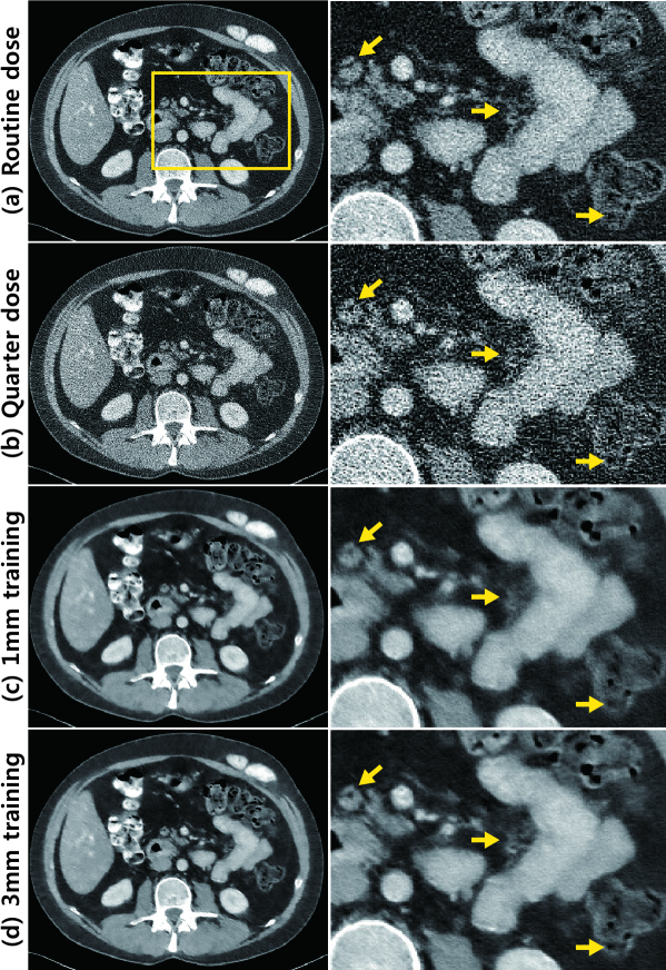
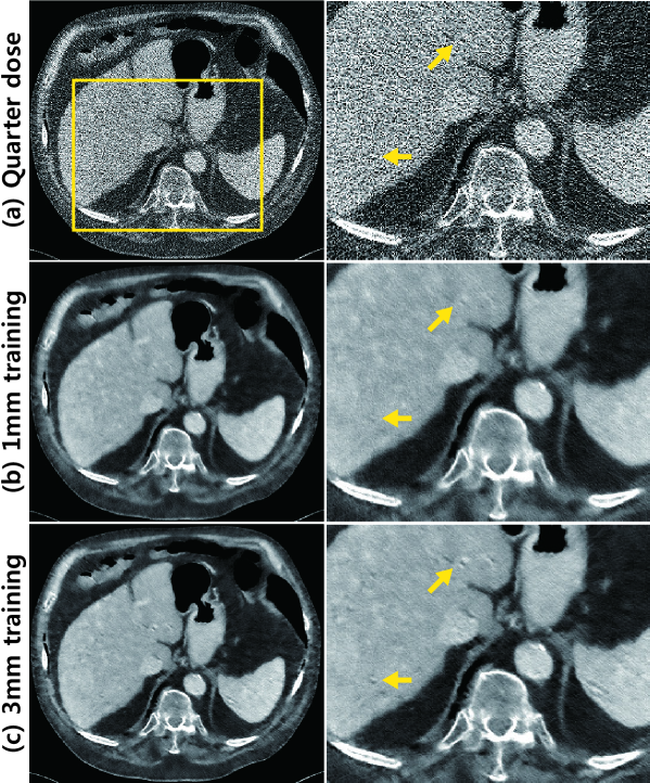
First, the comparative results from the 1mm and 3mm training data are shown in Fig. 6 and Fig. 7. The denoised images through the newly trained network with 3mm images preserve the fine image details better than those of the previous network. In particular, the image edges, such as the boundaries and details of the organs, become clearer. Although the denoised images, trained with 1mm slices, retained the details of the regions with lesions and significantly suppress the streaking artifacts, we found that the denoised images appeared somewhat blurred and that some high-frequency textures were often lost. This limitation resulted from the fact that the normal-dose CT images with a thickness of 1mm also contain noise, which reduces the accuracy of the supervised learning process.

With regard to the computation complexity, the proposed deep CNN framework is very advantageous; we showed that the average processing time for a 512 x 512 pixel CT image is approximately 1.6 seconds per slice for the MATLAB implementation with a dual-graphical processing unit (NVidia GeForce Titan 6GB). Accordingly, even a whole-body CT scan data can be processed by our method in a time frame of 2.1 $\sim$ 3.3 minutes, even when implemented on MATLAB. The calculation can be optimized further by optimizing the network architecture and the parallel computations and using a dedicated software platform for deep learning instead of MatConvNet.

Figure 8: X-ray CT images from training data set ‘L506’. Routine-dose images are in the first column, quarter-dose images are in the second column, and denoised images using the proposed algorithm are in the third column. (a) Transverse images. Enlarged images within the yellow box in the second row. The lesion is marked by red dashed circles. (b) Coronal images and (c) Sagittal images. The intensity range was set to (-160,240) [HU] (Hounsfield unit).

Figure 9: X-ray CT images from test data set ‘L057’. Quarter-dose images are in the first column and denoised images using the proposed algorithm are in the second column. (a) Transverse images. Enlarged images within the yellow box in the second row. The lesion is marked by red dashed circles. (b) Coronal images and (c) Sagittal images. Yellow arrow indicate the lesion. The intensity range was set to (-160,240) [HU] (Hounsfield unit).

Figure 10: X-ray CT images from test data set ‘L031’. Quarter-dose images are in the first column and denoised images using the proposed algorithm are in the second column. (a) Transverse images. Enlarged images within the yellow box in the second row. The intensity range has been adjusted to highlight the details of the lung. (b) Coronal images and (c) Sagittal images. Yellow arrows and circles indicate the details of the liver.

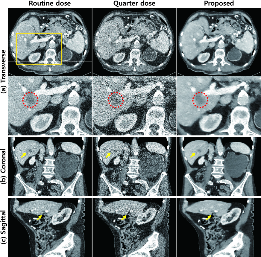
For a subjective evaluation, Fig. 8 shows the denoised images from the data set of one patient with a normal-dose and a quarter-dose. Organs such as the liver can be seen in these images. The results of the proposed network preserved the textures of the liver such that a better determination of the location of the lesion was possible, as highlighted by the red dashed circle. The coronal and sagittal presentation of the results is also shown in Fig. 8. Yellow arrows indicate the regions with high noise levels. The proposed network can remove a wide range of noise levels while maintaining the edge information.

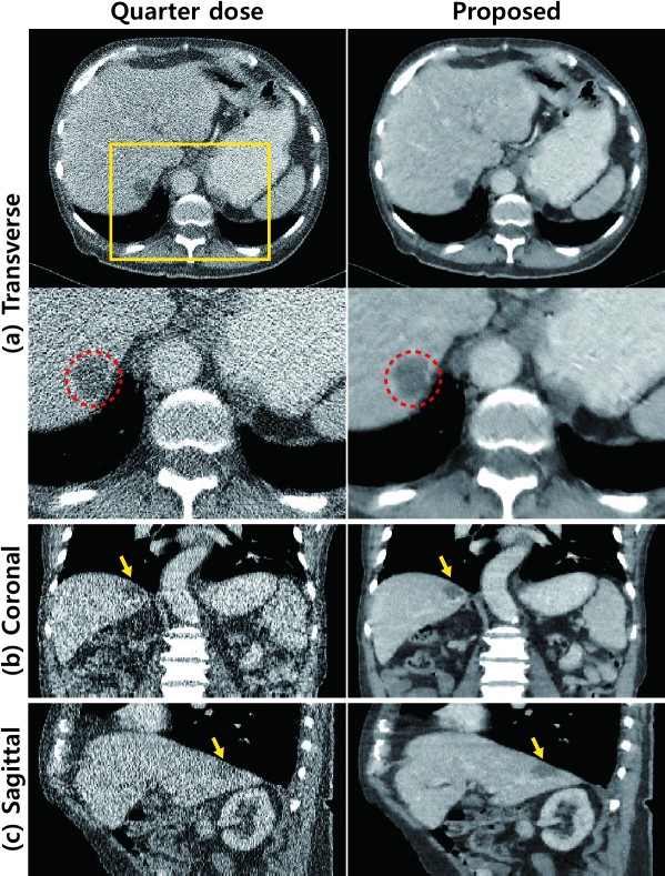
Fig. 9 shows the denoised images of data from one patient from among the 20 patients with only quarter-dose data. The trained network is applied to the test data and its denoising performance is demonstrated by the determination of the location of the lesion, as indicated by the red dashed circle. The coronal and sagittal presentation of the results is also shown in Fig. 9. Yellow arrows indicate the location of the lesion, providing a better view to assist with the understanding of the condition of the patient.

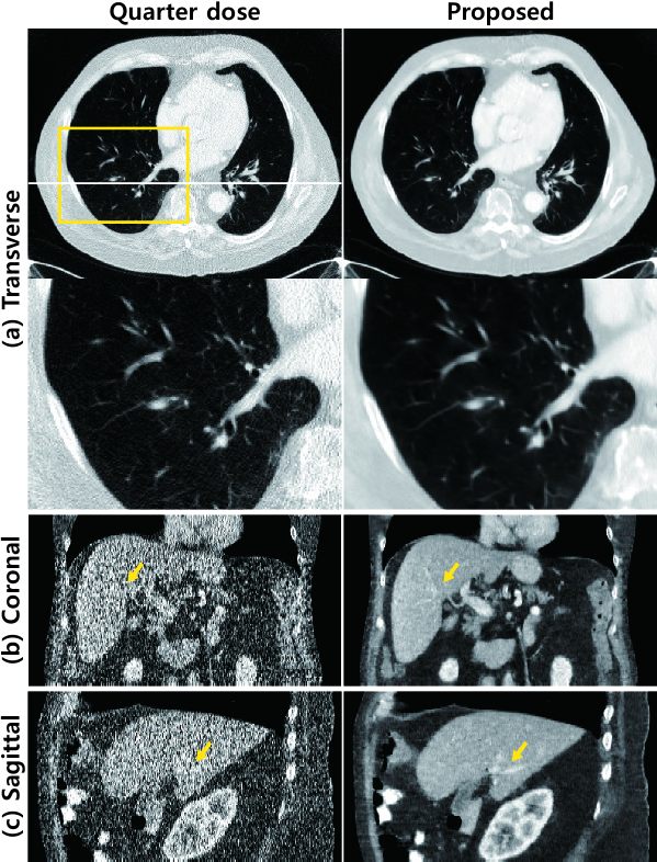
To demonstrate the detail preservation performance capabilities of the proposed network, we examine the results of another test data set, as shown in Fig. 10. The lung and other organs are visible in these images. The proposed network was able to describe the details of the lung structure. We also observed that the vessels in the liver are clearly reconstructed, as indicated by the yellow arrows in the coronal and sagittal presentation of the results.

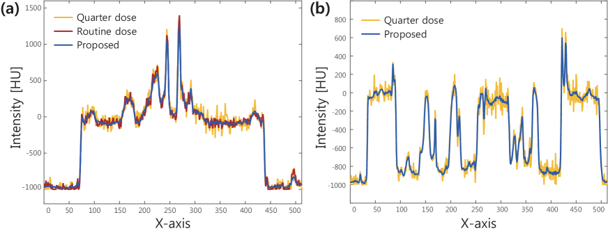
Profiles of the results are shown in Fig. 11 from both the training and the test data sets. Here, the corresponding positions of the profiles in Figs. 8 and 10 are indicated by white solid lines. In Fig. 11(a), the proposed network suitably reduces noise and describes the peak points. Moreover, the profiles of the results from the test data set in Fig. 11(b) show that the proposed network result also feasibly reduces noise in the test data.

Figure 11: (a) Intensity profile along the line in Fig. 8, and (b) Intensity profile along the line in Fig. 10

IV.2 Role of the wavelet transform

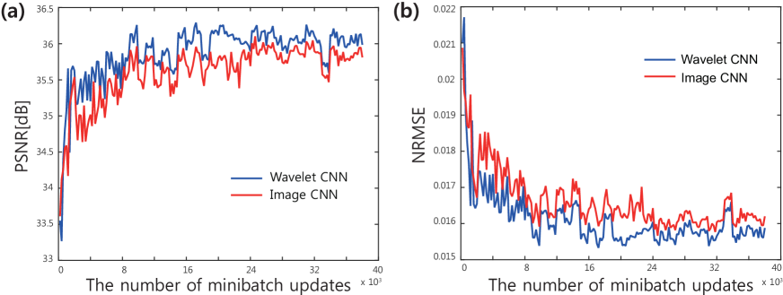
To verify the role of the wavelet transform, the proposed network was compared with a baseline CNN - an image-based neural network that is identical to the proposed network, except that its input and output layer are images. The baseline network was applied to the image patches instead of the local wavelet coefficients. These two networks were trained with the data from nine patients, and the remaining data from one patient was used for the evaluation. During the training process, the degrees of convergence were evaluated with the data from the one other patient. Fig. 12 shows that our wavelet-based CNN outperforms the image-domain CNN with regard to the peak signal-to-noise ratio (PSNR) and the normalized root mean square error (NRMSE).

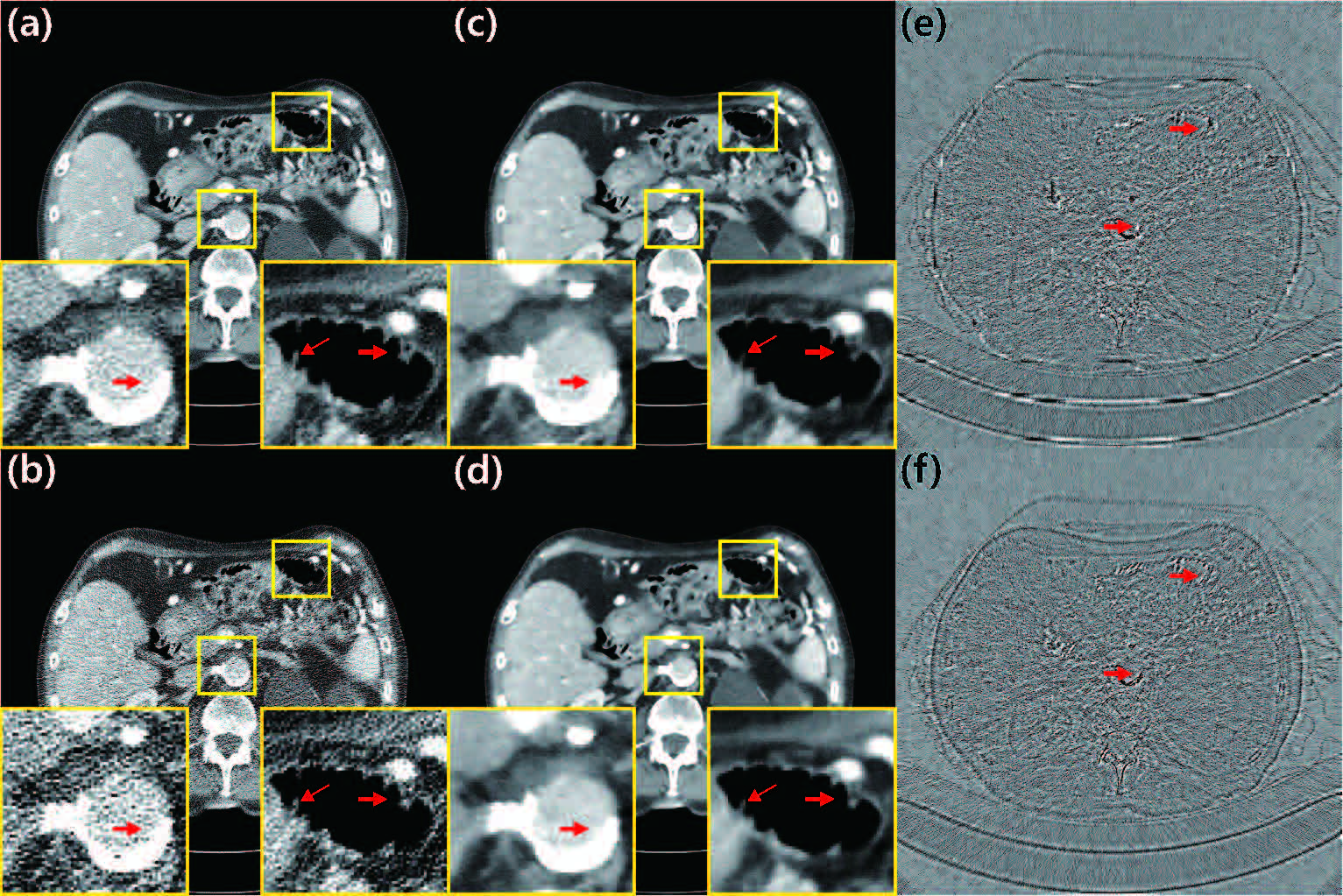
Fig. 13 illustrates the results of the proposed network and the image-domain CNN. The performance capabilities of the image-domain CNN were also impressive. On the other hand, the differences between the two were clearly visible in the images of difference, as they were mainly from the image edges. Moreover, many structures are not recovered in the image-domain CNN, as indicated by the red arrows in the yellow magnified boxes.

Figure 12: Comparison of the proposed network versus the image-domain CNN: (a) PSNR, and (b) NRMSE

Figure 13: Result images of the proposed network and the image-domain CNN: (a) Routine-dose image, (b) quarter-dose image, (c) image-domain CNN result, (d) the result from the proposed network, (e) the difference between the routine-dose and the image-domain CNN result, and (f) the difference between routine-dose and the proposed network result. The intensity range of the results was set to (-160,240) [HU], and the intensity range of the difference image was set to (-100,100) [HU].

IV.3 Analysis of residual learning techniques

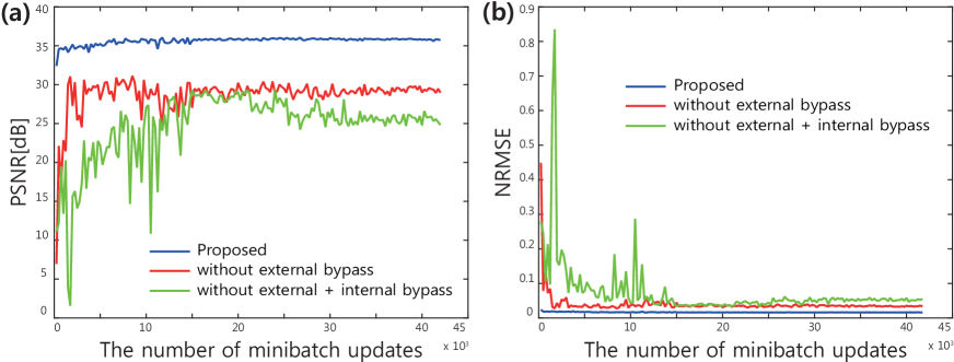
In order to verify the effect of the residual learning technique, the proposed network was compared with another baseline CNN with an identical architecture but without residual learning. The mapping between the contourlet coefficients of the lowest frequency band (level 4) was also learned in the baseline CNN (the red curve in Fig. 14). The comparison clearly shows the importance of residual learning.

Recall that in the proposed network, the input is added to the output before the ReLU layer in each module, and we combine the output of each module in the last step to form the concatenated layer, as shown in Fig. 5. Accordingly, we also analyzed the effectiveness of these internal bypass connections used in each module during the last step of the network. In Fig. 14, the proposed network is also compared to the baseline CNN, as designated by the green line, which does not have an external bypass path for low-frequency coefficients and internal bypass connections. Fig. 14 confirms that our unique residual learning architecture is helpful to train the proposed network.

Figure 14: Importance of residual learning: The proposed network is compared to a baseline network structure without an external low-frequency band bypass path and another baseline network without external bypass and internal bypass connections. Quantification by (a) PSNR, and (b) NRMSE.

V Discussion

An important advantage of the proposed network over MBIR approaches is that the proposed network can fully utilize a large training data set, if such a data set is available, given that a large number of neural network parameters can be trained more accurately with more data. On the other hand, MBIR approaches usually train a single regularization parameter despite the availability of a large training data set. Therefore, we believe that our method offers a significant advantage over MBIR approaches due to its ability to learn organ, protocol, and hardware-dependent noise from a larger available training data set.

In the 2016 CT low-dose Grand Challenge, only abdominal CT images with a quarter-dose were provided. Our network is adapted to a quarter-dose, while the noise distribution changes according to the dosage level. When we applied it to reconstruction from lower level noise, the denoised images contained blurring artifacts. Therefore, to enable a low-dose CT at another dose level, additional training with data with a different noise level will be required. However, transfer learning Taylor and Stone (2009); Yosinski et al. (2014); Pan and Yang (2010) or domain adaptationGanin et al. (2016) can now be considered feasible for use with deep learning. Thus, a pre-trained network can serve as the start point of training with another data set with different noise levels. This will reduce the training time and produce better results than training using a new data set only. Moreover, with regard to natural image de-noising, CNN networks are currently actively investigated for different noise levels. A previous study Burger, Schuler, and Harmeling (2012) demonstrated the possibility that a neural network can strongly remove various levels of noise. Similarly, if we have a multiple-dosage data set, we can train the network for different dose levels using all of the training samples from different noise levels. This type of heterogeneous training was shown to be effective in our recent work on deep-learning-based sparse view CT reconstruction Han, Yoo, and Ye (2016).

Projection domain de-noising has also been widely investigated for low-dose CT. Therefore, we can apply the proposed network to projection data. However, projection data is related across all angles, making the use of patch processing techniques more difficult. This difficulty can be overcome by a network with a large receptive field, similar to that in our recent workHan, Yoo, and Ye (2016), though this goes beyond the scope of the present work.

Finally, some of the radiologists who evaluated our results in the Low-dose CT Grand Challenge mentioned that the texture of our deep-learning reconstruction differs from those of MBIR methods. Because the textures of images are also important diagnostic features, a new deep-learning method is needed to deal with these problems as a follow-up study to this work.

VI Conclusion

In this paper, we introduced a deep CNN framework designed for low-dose CT reconstruction. It combines a deep convolution neural network with a directional wavelet approach. We demonstrated that the proposed method has greater de-noising power for low-dose CT and that its reconstruction time is much faster than those of MBIR methods. The effectiveness of the proposed network was confirmed in the 2016 AAPM Low-Dose CT Grand Challenge. We believe that the method presented here suggests a new innovative framework for low-dose CT research.

References

- Brenner and Hall (2007) D. J. Brenner and E. J. Hall, “Computed tomography: An increasing source of radiation exposure,” New England Journal of Medicine 357, 2277–2284 (2007)
- Yu et al. (2009) L. Yu, X. Liu, S. Leng, J. M. Kofler, J. C. Ramirez-Giraldo, M. Qu, J. Christner, J. G. Fletcher, and C. H. McCollough, “Radiation dose reduction in computed tomography: techniques and future perspective,” Imaging in Medicine 1, 65–84 (2009)
- Chambolle (2004) A. Chambolle, “An algorithm for total variation minimization and applications,” Journal of Mathematical Imaging and Vision 20, 89–97 (2004)
- Portilla et al. (2003) J. Portilla, V. Strela, M. J. Wainwright, and E. P. Simoncelli, “Image denoising using scale mixtures of Gaussians in the wavelet domain,” IEEE Transactions on Image Processing 12, 1338–1351 (2003)
- Crouse, Nowak, and Baraniuk (1998) M. S. Crouse, R. D. Nowak, and R. G. Baraniuk, “Wavelet-based statistical signal processing using hidden Markov models,” IEEE Transactions on Signal Processing 46, 886–902 (1998)
- Dabov et al. (2007) K. Dabov, A. Foi, V. Katkovnik, and K. Egiazarian, “Image denoising by sparse 3-D transform-domain collaborative filtering,” IEEE Transactions on Image Processing 16, 2080–2095 (2007)
- Kim et al. (2015) K. Kim, J. C. Ye, W. Worstell, J. Ouyang, Y. Rakvongthai, G. El Fakhri, and Q. Li, “Sparse-view spectral CT reconstruction using spectral patch-based low-rank penalty,” IEEE Transactions on Medical Imaging 34, 748–760 (2015)
- Hsieh (2003) J. Hsieh, Computed tomography: principles, design, artifacts, and recent advances, Vol. 114 (SPIE press, 2003)
- Beister, Kolditz, and Kalender (2012) M. Beister, D. Kolditz, and W. A. Kalender, “Iterative reconstruction methods in X-ray CT,” Physica Medica 28, 94–108 (2012)
- Ramani and Fessler (2012) S. Ramani and J. A. Fessler, “A splitting-based iterative algorithm for accelerated statistical X-ray CT reconstruction,” IEEE Transactions on Medical Imaging 31, 677–688 (2012)
- Kim, Ramani, and Fessler (2015) D. Kim, S. Ramani, and J. A. Fessler, “Combining ordered subsets and momentum for accelerated X-ray CT image reconstruction,” IEEE Transactions on Medical Imaging 34, 167–178 (2015)
- Xu et al. (2012) Q. Xu, H. Yu, X. Mou, L. Zhang, J. Hsieh, and G. Wang, “Low-dose X-ray CT reconstruction via dictionary learning,” IEEE Transactions on Medical Imaging 31, 1682–1697 (2012)
- Wieczorek et al. (2015) M. Wieczorek, J. Frikel, J. Vogel, E. Eggl, F. Kopp, P. B. Noël, F. Pfeiffer, L. Demaret, and T. Lasser, “X-ray computed tomography using curvelet sparse regularization,” Medical Physics 42, 1555–1565 (2015)
- Zhang et al. (2015) H. Zhang, J. Ma, J. Wang, Y. Liu, H. Han, H. Lu, W. Moore, and Z. Liang, “Statistical image reconstruction for low-dose CT using nonlocal means-based regularization. part ii: An adaptive approach,” Computerized Medical Imaging and Graphics 43, 26–35 (2015)
- Cho and Fessler (2015) J. H. Cho and J. A. Fessler, “Regularization designs for uniform spatial resolution and noise properties in statistical image reconstruction for 3-D X-ray CT,” IEEE Transactions on Medical Imaging 34, 678–689 (2015)
- Zhang and Salari (2005) S. Zhang and E. Salari, “Image denoising using a neural network based non-linear filter in wavelet domain,” in Proceedings.(ICASSP’05). IEEE International Conference on Acoustics, Speech, and Signal Processing, 2005., Vol. 2 (IEEE, 2005) pp. ii/989–ii/992
- Jain and Seung (2009) V. Jain and S. Seung, “Natural image denoising with convolutional networks,” in Advances in Neural Information Processing Systems 21 (Curran Associates, Inc., 2009) pp. 769–776
- Nasri and Nezamabadi-pour (2009) M. Nasri and H. Nezamabadi-pour, “Image denoising in the wavelet domain using a new adaptive thresholding function,” Neurocomputing 72, 1012–1025 (2009)
- Vincent et al. (2010) P. Vincent, H. Larochelle, I. Lajoie, Y. Bengio, and P.-A. Manzagol, “Stacked denoising autoencoders: Learning useful representations in a deep network with a local denoising criterion,” Journal of Machine Learning Research 11, 3371–3408 (2010)
- Burger, Schuler, and Harmeling (2012) H. C. Burger, C. J. Schuler, and S. Harmeling, “Image denoising: Can plain neural networks compete with BM3D?” in The IEEE Conference on Computer Vision and Pattern Recognition (CVPR) (IEEE, 2012) pp. 2392–2399
- Xie, Xu, and Chen (2012) J. Xie, L. Xu, and E. Chen, “Image denoising and inpainting with deep neural networks,” in Advances in Neural Information Processing Systems 25 (Curran Associates, Inc., 2012) pp. 341–349
- Mao, Shen, and Yang (2016) X. Mao, C. Shen, and Y. Yang, “Image denoising using very deep fully convolutional encoder-decoder networks with symmetric skip connections,” arXiv preprint arXiv:1603.09056 (2016)
- Chen, Yu, and Pock (2015) Y. Chen, W. Yu, and T. Pock, “On learning optimized reaction diffusion processes for effective image restoration,” in The IEEE Conference on Computer Vision and Pattern Recognition (CVPR) (IEEE, 2015) pp. 5261–5269
- Dong et al. (2014) C. Dong, C. C. Loy, K. He, and X. Tang, “Learning a deep convolutional network for image super-resolution,” in European Conference on Computer Vision (Springer, 2014) pp. 184–199
- Kim, Kwon Lee, and Mu Lee (2016) J. Kim, J. Kwon Lee, and K. Mu Lee, “Accurate image super-resolution using very deep convolutional networks,” in The IEEE Conference on Computer Vision and Pattern Recognition (CVPR) (IEEE, 2016)
- Zhou, Cunha, and Do (2005) J. Zhou, A. L. Cunha, and M. N. Do, “Nonsubsampled contourlet transform: construction and application in enhancement,” in IEEE International Conference on Image Processing 2005, Vol. 1 (IEEE, 2005) pp. I–469–742
- Ioffe and Szegedy (2015) S. Ioffe and C. Szegedy, “Batch normalization: Accelerating deep network training by reducing internal covariate shift,” arXiv preprint arXiv:1502.03167 (2015)
- Ioffe (2017) S. Ioffe, “Batch renormalization: Towards reducing minibatch dependence in batch-normalized models,” arXiv preprint arXiv:1702.03275 (2017)
- Nair and Hinton (2010) V. Nair and G. E. Hinton, “Rectified linear units improve restricted boltzmann machines,” in Proceedings of the 27th International Conference on Machine Learning (ICML-10) (2010) pp. 807–814
- He et al. (2016) K. He, X. Zhang, S. Ren, and J. Sun, “Deep residual learning for image recognition,” in The IEEE Conference on Computer Vision and Pattern Recognition (CVPR) (IEEE, 2016) pp. 770–778
- McCollough (2016) C. McCollough, “Low Dose CT Grand Challenge, the Mayo Clinic, the American Association of Physicists in Medicine, and grants EB017095 and grants EB017185 from the National Institute of Biomedical Imaging and Bioengineering,” (2016)
- Elad and Aharon (2006) M. Elad and M. Aharon, “Image denoising via sparse and redundant representations over learned dictionaries,” IEEE Transactions on Image Processing 15, 3736–3745 (2006)
- Krizhevsky, Sutskever, and Hinton (2012) A. Krizhevsky, I. Sutskever, and G. E. Hinton, “ImageNet classification with deep convolutional neural networks,” in Advances in Neural Information Processing Systems 25 (Curran Associates, Inc., 2012) pp. 1097–1105
- Cotter et al. (2011) A. Cotter, O. Shamir, N. Srebro, and K. Sridharan, “Better mini-batch algorithms via accelerated gradient methods,” in Advances in Neural Information Processing Systems 24 (Curran Associates, Inc., 2011) pp. 1647–1655
- Ronneberger, Fischer, and Brox (2015) O. Ronneberger, P. Fischer, and T. Brox, “U-net: Convolutional networks for biomedical image segmentation,” in International Conference on Medical Image Computing and Computer-Assisted Intervention - MICCAI 2015 (Springer, 2015) pp. 234–241
- Suzuki (2012) K. Suzuki, “Pixel-based machine learning in medical imaging,” Journal of Biomedical Imaging 2012, 1 (2012)
- Donoho (1995) D. L. Donoho, “De-noising by soft-thresholding,” IEEE Transactions on Information Theory 41, 613–627 (1995)
- Rumelhart, Hinton, and Williams (1986) D. E. Rumelhart, G. E. Hinton, and R. J. Williams, “Learning representations by back-propagating errors,” Nature 323, 533–538 (1986)
- Zhang (2004) T. Zhang, “Solving large scale linear prediction problems using stochastic gradient descent algorithms,” in Proceedings of the Twenty-first International Conference on Machine Learning, ICML ’04 (ACM, 2004) p. 116
- Vedaldi and Lenc (2015) A. Vedaldi and K. Lenc, “MatConvNet: Convolutional neural networks for MATLAB,” in Proceedings of the 23rd ACM International Conference on Multimedia (ACM, 2015) pp. 689–692
- Flohr et al. (2005) T. Flohr, K. Stierstorfer, S. Ulzheimer, H. Bruder, A. Primak, and C. H. McCollough, “Image reconstruction and image quality evaluation for a 64-slice CT scanner with z-flying focal spot,” Medical Physics 32, 2536–2547 (2005)
- Noo, Defrise, and Clackdoyle (1999) F. Noo, M. Defrise, and R. Clackdoyle, “Single-slice rebinning method for helical cone-beam CT,” Physics in Medicine and Biology 44, 561 (1999)
- Taylor and Stone (2009) M. E. Taylor and P. Stone, “Transfer learning for reinforcement learning domains: A survey,” Journal of Machine Learning Research 10, 1633–1685 (2009)
- Yosinski et al. (2014) J. Yosinski, J. Clune, Y. Bengio, and H. Lipson, “How transferable are features in deep neural networks?” in Advances in Neural Information Processing Systems 27 (Curran Associates, Inc., 2014) pp. 3320–3328
- Pan and Yang (2010) S. J. Pan and Q. Yang, “A survey on transfer learning,” IEEE Transactions on Knowledge and Data Engineering 22, 1345–1359 (2010)
- Ganin et al. (2016) Y. Ganin, E. Ustinova, H. Ajakan, P. Germain, H. Larochelle, F. Laviolette, M. Marchand, and V. Lempitsky, “Domain-adversarial training of neural networks,” Journal of Machine Learning Research 17, 1–35 (2016)
- Han, Yoo, and Ye (2016) Y. Han, J. Yoo, and J. C. Ye, “Deep residual learning for compressed sensing CT reconstruction via persistent homology analysis,” arXiv preprint arXiv:1611.06391 (2016)