Community detection with nodal information

Haolei Wenglabel=e1]hw2375@columbia.edu [    Yang Fenglabel=e2]yang.feng@columbia.edu [ Columbia University Department of Statistics,
Columbia University,
New York, NY, 10027.

E-mail: e2
Abstract

Community detection is one of the fundamental problems in the study of network data. Most existing community detection approaches only consider edge information as inputs, and the output could be suboptimal when nodal information is available. In such cases, it is desirable to leverage nodal information for the improvement of community detection accuracy. Towards this goal, we propose a flexible network model incorporating nodal information, and develop likelihood-based inference methods. For the proposed methods, we establish favorable asymptotic properties as well as efficient algorithms for computation. Numerical experiments show the effectiveness of our methods in utilizing nodal information across a variety of simulated and real network data sets.

62F99,
62P25.,
Networks,
Community detection,
Stochastic block model,
Multi-logistic regression,
Maximum likelihood,
Profile likelihood,
Variational inference,
Consistency,
Semidefinite programming.,
keywords:
[class=AMS]
keywords:
\startlocaldefs\endlocaldefs

and t2Partially supported by NSF CAREER Grant DMS-1554804.

1 Introduction.

Networked systems are ubiquitous in modern society. Examples include worldwide web, gene regulatory networks, and social networks. Network analysis has attracted a lot of research attention from social science, physics, computer science and mathematical science. There have been some interesting findings regarding the network structures, such as small world phenomena and power-law degree distributions (Newman, 2003). One of the fundamental problems in network analysis is detecting and characterizing community structure in networks. Communities can be intuitively understood as groups of nodes which are densely connected within groups while sparsely connected between groups111More rarely, one can encounter communities of the opposite meaning in disassortative mixing networks.. Identifying network communities not only helps better understand structural features of the network, but also offers practical benefits. For example, communities in social networks tend to share similar interest, which could provide useful information to build recommendation systems.

Existing community detection methods can be roughly divided into algorithmic and model-based ones (Zhao et al., 2012). Algorithmic methods typically define an objective function such as modularity (Newman, 2006), which measures the goodness of a network partition, and design algorithms to search for the solution of the corresponding optimization problem. See Fortunato (2010) for a thorough discussion of various algorithms. Unlike algorithmic approaches, model-based methods first construct statistical models that are assumed to generate the networks under study, and then develop statistical inference tools to learn the latent communities. Some popular models include stochastic block model (Holland et al., 1983), degree-corrected stochastic block model (Dasgupta et al., 2004; Karrer and Newman, 2011) and mixed membership stochastic block model (Airoldi et al., 2009).

In recent years, there have been increasingly active researches towards understanding the theoretical performances of community detection methods under different types of models. Regarding the stochastic block model, consistency results have been proved for likelihood based approaches, including maximum likelihood (Celisse et al., 2012; Choi et al., 2012), profile likelihood (Bickel and Chen, 2009), pseudo likelihood (Amini et al., 2013) and variational inference (Celisse et al., 2012; Bickel et al., 2013), among others. Some of the existing results are generalized to degree-corrected block models (Zhao et al., 2012). Another line of theoretical works focuses on methods of moments. See Rohe et al. (2011); Lei and Rinaldo (2014); Jin (2015); Qin and Rohe (2013); Joseph and Yu (2013) on theoretical analysis of spectral clustering for detecting communities in block models. Spectral clustering (Zhang et al., 2014) and tensor spectral method (Anandkumar et al., 2014) have also been used to detect overlapping communities under mixed membership models. In addition, carefully constructed convex programming has been shown to enjoy provable guarantees for community detection (Chen et al., 2012; Amini and Levina, 2014; Cai and Li, 2015; Guédon and Vershynin, 2016; Chen et al., 2015). See also the interesting theoretical works of community detection under minimax framework (Zhang and Zhou, 2015; Gao et al., 2015). Finally, there exists a different research theme focusing on detectability instead of consistency (Decelle et al., 2011; Krzakala et al., 2013; Saade et al., 2014; Abbe and Sandon, 2015).

All the aforementioned methods are based on only the observations of the edge connections in the networks. In the real world, however, networks often appear with additional nodal information. For example, social networks such as Facebook and Twitter contain users’ personal profile information. A citation network has the authors’ names, keywords, and abstracts of papers. Since nodes in the same communities tend to share similar features, we can expect that nodal attributes are in turn indicative of community structures. Combining both sources of edge and nodal information opens the possibility for more accurate community discovery. Many efficient heuristic algorithms are proposed in recent years to accomplish this goal (Akoglu et al., 2012; Ruan et al., 2013; Chang and Blei, 2010; Nallapati and Cohen, 2008; Yang et al., 2013). However, not much theory has been established to understand the statistical properties. See Binkiewicz et al. (2014); Zhang et al. (2013) for some theoretical developments. In this paper, we aim to give a thorough study of the community detection with nodal information problem. Our work first introduces a flexible modeling framework tuned for community detection when edge and nodal information coexist. Under a specific model, we then study three likelihood methods and derive their asymptotic properties. Regarding the computation of the estimators, we resort to a convex relaxation (semidefinite programming) approach to obtain a preliminary community estimate serving as a good initialization fed into “coordinate” ascent type iterative algorithms, to help locate the global optima. Various numerical experiments demonstrate that our methods can accurately discover community structures by making efficient use of nodal information.

The rest of the paper is organized as follows. Section 2 introduces our network model with nodal information. We then propose likelihood based methods and derive the corresponding asymptotic properties in Section 3. Section 4 is devoted to the design and analysis of practical algorithms. Simulation examples and real data analysis are presented in Section 5. We conclude the paper with a discussion in Section 6. All the technical proofs are collected in the Appendix.

2 Network Modeling with Nodal Information.

A network is usually represented by a graph G(V,E)𝐺𝑉𝐸G(V,E), where V={1,2,,n}𝑉12𝑛V=\{1,2,\dots,n\} is the set of nodes and E𝐸E is the set of edges. Throughout the paper, we will focus on the networks in which the corresponding graphs are undirected and contain no self-edges. The observed edge information can be recorded in the adjacency matrix A{0,1}n×n𝐴superscript01𝑛𝑛A\in\{0,1\}^{n\times n}, where Aij=Aji=1subscript𝐴𝑖𝑗subscript𝐴𝑗𝑖1A_{ij}=A_{ji}=1 if and only if (i,j)E𝑖𝑗𝐸(i,j)\in E. Suppose the network can be divided into K𝐾K non-overlapping communities. Let 𝒄=(c1,,cn)𝒄subscript𝑐1subscript𝑐𝑛\bm{c}=(c_{1},\dots,c_{n}) be the community assignment vector, with cisubscript𝑐𝑖c_{i} denoting the community membership of node i𝑖i and taking values in {1,2,,K}12𝐾\{1,2,\dots,K\}. Additionally, the available nodal information is formulated in a covariate matrix X=(𝒙1,,𝒙n)Tn×p𝑋superscriptsubscript𝒙1subscript𝒙𝑛𝑇superscript𝑛𝑝X=(\bm{x}_{1},\dots,\bm{x}_{n})^{T}\in\mathbb{R}^{n\times p}, where 𝒙ipsubscript𝒙𝑖superscript𝑝\bm{x}_{i}\in\mathbb{R}^{p} is the i𝑖i-th node’s covariate vector. The goal is to estimate 𝒄𝒄\bm{c} from the observations A𝐴A and X𝑋X.

2.1 Conditional Independence.

We treat A,X𝐴𝑋A,X and 𝒄𝒄\bm{c} as random and posit a statistical model for them. Before introducing the model, we would like to elucidate the main motivation. For the purpose of community detection, we follow the standard two-step inference procedure:

  • (1)

    Derive parameter estimator 𝜽^^𝜽\hat{\bm{\theta}} based on P(A,X;𝜽)𝑃𝐴𝑋𝜽P(A,X;\bm{\theta}),

  • (2)

    Perform posterior inference according to P(𝒄A,X;𝜽^)𝑃conditional𝒄𝐴𝑋^𝜽P(\bm{c}\mid A,X;\hat{\bm{\theta}}).

Under this framework, we now make a conditional independence assumption: AX𝐜perpendicular-to𝐴conditional𝑋𝐜A\perp X\mid\bm{c}. Admittedly, the assumption imposes a strong constraint that given the community membership, what nodes are like (described by covariates X𝑋X) does not affect how they are connected (encoded in A𝐴A). On the other hand, this assumption is consistent with our belief that knowing nodal information can help identify community structure 𝒄𝒄\bm{c}. More importantly, this assumed conditional independence turns out to simplify the above two steps to a great extent. First, for the parameter estimation step, the conditional independence assumption implies that

P(A,X;𝜽)=𝒄P(A𝒄)P(X𝒄)P(𝒄)=P(X;𝜽1)𝒄P(A𝒄;𝜽2)P(𝒄X;𝜽3),𝑃𝐴𝑋𝜽subscript𝒄𝑃conditional𝐴𝒄𝑃conditional𝑋𝒄𝑃𝒄𝑃𝑋subscript𝜽1subscript𝒄𝑃conditional𝐴𝒄subscript𝜽2𝑃conditional𝒄𝑋subscript𝜽3\displaystyle P(A,X;\bm{\theta})=\sum_{\bm{c}}P(A\mid\bm{c})P(X\mid\bm{c})P(\bm{c})=P(X;\bm{\theta}_{1})\sum_{\bm{c}}P(A\mid\bm{c};\bm{\theta}_{2})P(\bm{c}\mid X;\bm{\theta}_{3}), (1)

where 𝜽=(𝜽1,𝜽2,𝜽3)𝜽subscript𝜽1subscript𝜽2subscript𝜽3\bm{\theta}=(\bm{\theta}_{1},\bm{\theta}_{2},\bm{\theta}_{3}) indexes a family of generative models (not restricted to parametric forms). Regarding the second step, conditional independence leads to

P(𝒄A,X)𝑃conditional𝒄𝐴𝑋\displaystyle P(\bm{c}\mid A,X) =P(A𝒄)P(X𝒄)P(𝒄)𝒄P(A𝒄)P(X𝒄)P(𝒄)=P(A𝒄)P(𝒄X)P(X)𝒄P(A𝒄)P(𝒄X)P(X)absent𝑃conditional𝐴𝒄𝑃conditional𝑋𝒄𝑃𝒄subscript𝒄𝑃conditional𝐴𝒄𝑃conditional𝑋𝒄𝑃𝒄𝑃conditional𝐴𝒄𝑃conditional𝒄𝑋𝑃𝑋subscript𝒄𝑃conditional𝐴𝒄𝑃conditional𝒄𝑋𝑃𝑋\displaystyle=\frac{P(A\mid\bm{c})P(X\mid\bm{c})P(\bm{c})}{\sum_{\bm{c}}P(A\mid\bm{c})P(X\mid\bm{c})P(\bm{c})}=\frac{P(A\mid\bm{c})P(\bm{c}\mid X)P(X)}{\sum_{\bm{c}}P(A\mid\bm{c})P(\bm{c}\mid X)P(X)} (2)
=P(A𝒄)P(𝒄X)𝒄P(A𝒄)P(𝒄X).absent𝑃conditional𝐴𝒄𝑃conditional𝒄𝑋subscript𝒄𝑃conditional𝐴𝒄𝑃conditional𝒄𝑋\displaystyle=\frac{P(A\mid\bm{c})P(\bm{c}\mid X)}{\sum_{\bm{c}}P(A\mid\bm{c})P(\bm{c}\mid X)}.

From (1) and (2), we observe that the distribution P(X)𝑃𝑋P(X) is a “nuisance” in the two-step procedure. Hence we are able to avoid modeling and estimating the marginal distribution of X𝑋X. As a result, the effort can be saved for the inference of P(A𝒄)𝑃conditional𝐴𝒄P(A\mid\bm{c}) and P(𝒄X)𝑃conditional𝒄𝑋P(\bm{c}\mid X).

2.2 Node-coupled Stochastic Block Model.

The conditional independence and follow-up arguments in Section 2.1 pave the way to a flexible framework of models for networks with nodal covariates: specifying the two conditionals P(A𝒄)𝑃conditional𝐴𝒄P(A\mid\bm{c}) and P(𝒄X)𝑃conditional𝒄𝑋P(\bm{c}\mid X). A similar modeling strategy was proposed in Newman and Clauset (2015), along with detailed empirical results. Unlike them, we will consider a different model and present a thorough study from both theoretical and computational perspectives. Note that the conditional distribution P(A𝒄)𝑃conditional𝐴𝒄P(A\mid\bm{c}) only involves the edge information of the network, while P(𝒄X)𝑃conditional𝒄𝑋P(\bm{c}\mid X) is often encountered in the standard regression setting for i.i.d. data. This motivates us to consider the following model.

Node-coupled Stochastic Block Model (NSBM):

  • (a)

    P(A𝒄)=i<jBcicjAij(1Bcicj)1Aij𝑃conditional𝐴𝒄𝑖𝑗productsuperscriptsubscript𝐵subscript𝑐𝑖subscript𝑐𝑗subscript𝐴𝑖𝑗superscript1subscript𝐵subscript𝑐𝑖subscript𝑐𝑗1subscript𝐴𝑖𝑗P(A\mid\bm{c})=\underset{i<j}{\prod}B_{c_{i}c_{j}}^{A_{ij}}(1-B_{c_{i}c_{j}})^{1-A_{ij}},

  • (b)

    P(𝒄X)=𝑖exp(𝜷ciT𝒙i)k=1Kexp(𝜷kT𝒙i)𝑃conditional𝒄𝑋𝑖productsubscriptsuperscript𝜷𝑇subscript𝑐𝑖subscript𝒙𝑖superscriptsubscript𝑘1𝐾subscriptsuperscript𝜷𝑇𝑘subscript𝒙𝑖P(\bm{c}\mid X)=\underset{i}{\prod}\frac{\exp(\bm{\beta}^{T}_{c_{i}}\bm{x}_{i})}{\sum_{k=1}^{K}\exp({\bm{\beta}^{T}_{k}\bm{x}_{i}})},

where B=(Bab)[0,1]K×K𝐵subscript𝐵𝑎𝑏superscript01𝐾𝐾B=(B_{ab})\in[0,1]^{K\times K} is symmetric, 𝜷=(𝜷1,,𝜷K)Kp𝜷subscript𝜷1subscript𝜷𝐾superscript𝐾𝑝\bm{\beta}=(\bm{\beta}_{1},\dots,\bm{\beta}_{K})\in\mathbb{R}^{Kp}. The distribution P(A𝒄)𝑃conditional𝐴𝒄P(A\mid\bm{c}) in (a) follows the stochastic block model (SBM), which, as the fundamental model, has been extensively studied in the literature. The SBM implies that the distribution of an edge between node i𝑖i and j𝑗j only depends on their community membership cisubscript𝑐𝑖c_{i} and cjsubscript𝑐𝑗c_{j}. The nodes from the same community are stochastically equivalent. The element Babsubscript𝐵𝑎𝑏B_{ab} in the matrix B𝐵B represents the probability of edge connection between a node in community a𝑎a and a node in community b𝑏b. The P(𝒄X)𝑃conditional𝒄𝑋P(\bm{c}\mid X) in (b) simply takes a multi-logistic regression form, where we will assume 𝜷K=𝟎subscript𝜷𝐾0\bm{\beta}_{K}=\bm{0} for identifiability. Simple as it looks, we would like to point out some advantages of NSBM:

  • The parameters in NSBM can be estimated by combining the estimation of B𝐵B under (a) and 𝜷𝜷\bm{\beta} under (b), as we shall elaborate in Section 4.

  • The coefficient 𝜷𝜷\bm{\beta} reflects the contribution of each nodal covariate for identifying community structures. This information can help us better understand the implication of the network communities.

  • The probability p(c=k𝒙)=exp(𝜷kT𝒙)k=1Kexp(𝜷kT𝒙)𝑝𝑐conditional𝑘𝒙subscriptsuperscript𝜷𝑇𝑘𝒙superscriptsubscript𝑘1𝐾subscriptsuperscript𝜷𝑇𝑘𝒙p(c=k\mid\bm{x})=\frac{\exp({\bm{\beta}^{T}_{k}\bm{x}})}{\sum_{k=1}^{K}\exp({\bm{\beta}^{T}_{k}\bm{x}})} can be used to predict a new node’s community membership c𝑐c based on its covariates 𝒙𝒙\bm{x}, without waiting for it to form network connections.

  • Both P(A𝒄)𝑃conditional𝐴𝒄P(A\mid\bm{c}) and P(𝒄X)𝑃conditional𝒄𝑋P(\bm{c}\mid X) can be readily generalized to fit more complicated structures.

Remark 1.

As illustrated in Section 2.1, under the conditional independence assumption AX𝐜perpendicular-to𝐴conditional𝑋𝐜A\perp X\mid\bm{c}, it is sufficient to consider the conditional likelihood P(A,𝐜X)𝑃𝐴conditional𝐜𝑋P(A,\bm{c}\mid X) instead of the full version P(A,𝐜,X)𝑃𝐴𝐜𝑋P(A,\bm{c},X). In particular, we study the maximum likelihood estimate, maximum variational likelihood estimate, and the maximum profile likelihood estimate based on the conditional likelihood in the next section. However, we emphasize that the conditional independence assumption is not part of NSBM, though it was used to motivate the model. In the next section, we will treat this assumption as working independence to derive the likelihood based estimates. Hence, the three estimates are in fact based on pseudo likelihood. With a slight abuse of terminology and for simplicity, we still call them the aforementioned likelihood names in the rest of the paper.

3 Statistical Inference under NSBM.

For community detection, our main goal is to find an accurate community assignment estimator 𝒄^^𝒄\hat{\bm{c}} for the underlying true communities 𝒄𝒄\bm{c}. Theoretically, we would like to study the consistency of community detection for a given method. We adopt the notions of consistency from Bickel and Chen (2009) and Zhao et al. (2012):

(strong consistency)strong consistency\displaystyle(\mbox{\emph{strong consistency}}) P(𝒄^=𝒄)1, as n,formulae-sequence𝑃^𝒄𝒄1 as 𝑛\displaystyle P(\hat{\bm{c}}=\bm{c})\rightarrow 1,\mbox{~{}as~{}}n\rightarrow\infty,
(weak consistency)weak consistency\displaystyle(\mbox{\emph{weak consistency}}) ϵ>0,P(1ni=1n𝟙(c^ici)<ϵ)1, as n.formulae-sequencefor-allitalic-ϵ0formulae-sequence𝑃1𝑛superscriptsubscript𝑖1𝑛1subscript^𝑐𝑖subscript𝑐𝑖italic-ϵ1 as 𝑛\displaystyle\forall\epsilon>0,P\Big{(}\frac{1}{n}\sum_{i=1}^{n}\mathbbm{1}(\hat{c}_{i}\neq c_{i})<\epsilon\Big{)}\rightarrow 1,\mbox{~{}as~{}}n\rightarrow\infty.

As the network size increases to infinity, with probability approaching 1, strong consistency requires perfect recovery of the true community structure, while weak consistency only needs the mis-classification rate to be arbitrarily small. Note that since community structure is invariant under a permutation of the community labels in {1,2,,K}12𝐾\{1,2,\dots,K\}, the consistency notations above as well as the estimators to be introduced should always be interpreted up to label permutations.

In the asymptotic setting where the network size n𝑛n\rightarrow\infty, holding the parameter B[0,1]K×K𝐵superscript01𝐾𝐾B\in[0,1]^{K\times K} unchanged implies that the total number of edges present in the network is of order O(n2)𝑂superscript𝑛2O(n^{2}). Such networks are unrealistically dense. To study under a more realistic asymptotic framework, we allow B𝐵B to change with n𝑛n. In particular, we consider a sequence of submodels where B=ρnB¯𝐵subscript𝜌𝑛¯𝐵B=\rho_{n}\bar{B} with B¯¯𝐵\bar{B} fixed and ρn=P(Aij=1)0subscript𝜌𝑛𝑃subscript𝐴𝑖𝑗10\rho_{n}=P(A_{ij}=1)\rightarrow 0 as n𝑛n\rightarrow\infty. The same asymptotic formulation was studied in Bickel and Chen (2009); Zhao et al. (2012); Bickel et al. (2013). In this way, the parameter ρnsubscript𝜌𝑛\rho_{n} directly represents the sparsity level of the network. For the consistency results to be derived in the subsequent sections, we will specify the sufficient conditions on the order of ρnsubscript𝜌𝑛\rho_{n}.

As pointed out in Section 2.2, the parameter 𝜷𝜷\bm{\beta} in NSBM is associated with the contribution of each nodal covariate for discovering communities. Measuring the importance of each nodal attribute to the community structure may provide insightful information about the network. For that purpose, in addition to community detection, we will study the asymptotics of the estimators for 𝜷𝜷\bm{\beta} as well. Since the parameter B𝐵B is not of current interest, we will skip the theoretical analysis of the corresponding estimators.

3.1 Consistency of Maximum Likelihood Method.

In Section 2.1, we pointed out the appealing implication of the assumed conditional independence for likelihood based inference procedure. We now evaluate this procedure under the asymptotic framework we introduced at the beginning of Section 3. Towards that end, we define the following maximum likelihood based estimators222Recall that the likelihood formulation is the pseudo version as pointed out in Remark 1. Similar explanations hold for the other two likelihood based methods presented in the subsequent sections. :

(𝜷^,B^)^𝜷^𝐵\displaystyle(\hat{\bm{\beta}},\hat{B}) =argmax𝜷K=𝟎,𝜷KpB[0,1]K×K,BT=B𝒄i<jBcicjAij(1Bcicj)1Aij𝑖exp(𝜷ciT𝒙i)k=1Kexp(𝜷kT𝒙i),absentsubscriptargmaxformulae-sequencesubscript𝜷𝐾0𝜷superscript𝐾𝑝formulae-sequence𝐵superscript01𝐾𝐾superscript𝐵𝑇𝐵subscript𝒄𝑖𝑗productsuperscriptsubscript𝐵subscript𝑐𝑖subscript𝑐𝑗subscript𝐴𝑖𝑗superscript1subscript𝐵subscript𝑐𝑖subscript𝑐𝑗1subscript𝐴𝑖𝑗𝑖productsubscriptsuperscript𝜷𝑇subscript𝑐𝑖subscript𝒙𝑖superscriptsubscript𝑘1𝐾subscriptsuperscript𝜷𝑇𝑘subscript𝒙𝑖\displaystyle=\operatorname*{arg\,max}_{\begin{subarray}{c}\bm{\beta}_{K}=\bm{0},~{}\bm{\beta}\in\mathbb{R}^{Kp}\\ B\in[0,1]^{K\times K},B^{T}=B\end{subarray}}\sum_{\bm{c}}~{}\underset{i<j}{\prod}B_{c_{i}c_{j}}^{A_{ij}}(1-B_{c_{i}c_{j}})^{1-A_{ij}}\cdot\underset{i}{\prod}\frac{\exp(\bm{\beta}^{T}_{c_{i}}\bm{x}_{i})}{\sum_{k=1}^{K}\exp({\bm{\beta}^{T}_{k}\bm{x}_{i}})}, (3)
𝒄^^𝒄\displaystyle\hat{\bm{c}} =argmax𝒄{1,,K}ni<jB^cicjAij(1B^cicj)1Aij𝑖exp(𝜷^ciT𝒙i)k=1Kexp(𝜷^kT𝒙i).absentsubscriptargmax𝒄superscript1𝐾𝑛𝑖𝑗productsuperscriptsubscript^𝐵subscript𝑐𝑖subscript𝑐𝑗subscript𝐴𝑖𝑗superscript1subscript^𝐵subscript𝑐𝑖subscript𝑐𝑗1subscript𝐴𝑖𝑗𝑖productsubscriptsuperscript^𝜷𝑇subscript𝑐𝑖subscript𝒙𝑖superscriptsubscript𝑘1𝐾subscriptsuperscript^𝜷𝑇𝑘subscript𝒙𝑖\displaystyle=\operatorname*{arg\,max}_{\bm{c}\in\{1,\dots,K\}^{n}}\underset{i<j}{\prod}\hat{B}_{c_{i}c_{j}}^{A_{ij}}(1-\hat{B}_{c_{i}c_{j}})^{1-A_{ij}}\cdot\underset{i}{\prod}\frac{\exp({\hat{\bm{\beta}}^{T}_{c_{i}}\bm{x}_{i}})}{\sum_{k=1}^{K}\exp({\hat{\bm{\beta}}^{T}_{k}\bm{x}_{i}})}. (4)

The estimators defined above are the realizations of the two-step procedure we mentioned at the beginning of Section 2.1. We are mainly interested in studying the consistency of 𝜷^^𝜷\hat{\bm{\beta}} and 𝒄^^𝒄\hat{\bm{c}}.

First, we would like to introduce several technical conditions.

Condition 1.

B¯¯𝐵\bar{B} has no two identical columns.

If the probability matrix B¯¯𝐵\bar{B} has two identical columns, then there exist at least two communities unidentifiable with each other. In practice, it makes sense to combine those communities into a bigger one.

Condition 2.

(c1,𝒙1),,(cn,𝒙n)iid(c,𝒙)subscript𝑐1subscript𝒙1subscript𝑐𝑛subscript𝒙𝑛𝑖𝑖𝑑similar-to𝑐𝒙(c_{1},\bm{x}_{1}),\dots,(c_{n},\bm{x}_{n})\overset{iid}{\sim}(c,\bm{x}) with 𝔼(𝐱𝐱T)0succeeds𝔼𝐱superscript𝐱𝑇0\mathbb{E}(\bm{x}\bm{x}^{T})\succ 0, where 0succeedsabsent0\succ 0 represents the matrix being positive definite.

Condition 2 ensures the coefficient vector 𝜷𝜷\bm{\beta} is uniquely identifiable.

Condition 3.

There exist constants κ1subscript𝜅1\kappa_{1} and κ2subscript𝜅2\kappa_{2} such that for sufficiently large t𝑡t, we have

P(𝒙2>t)κ1eκ2t.𝑃subscriptnorm𝒙2𝑡subscript𝜅1superscript𝑒subscript𝜅2𝑡P(\|\bm{x}\|_{2}>t)\leq\kappa_{1}e^{-\kappa_{2}t}.

Condition 3 imposes a sub-exponential tail bound on 𝒙2subscriptnorm𝒙2\|\bm{x}\|_{2}, which is equivalent to sub-exponential tail assumption on each component of 𝒙𝒙\bm{x}, via a simple union bound argument. This covers many different types of covariates like discrete, Gaussian and exponential.

Theorem 1.

Assume the data (A,X)𝐴𝑋(A,X) follows NSBM and Conditions 1, 2 and 3 hold. In addition, assume nρnlogn𝑛subscript𝜌𝑛𝑛\frac{n\rho_{n}}{\log n}\rightarrow\infty as n𝑛n\rightarrow\infty. Then, we have as n𝑛n\rightarrow\infty

P(𝒄^=𝒄)1,n(𝜷^𝜷)𝑑N(𝟎,I1(𝜷)),𝑃^𝒄𝒄1𝑛^𝜷𝜷𝑑𝑁0superscript𝐼1𝜷\displaystyle P(\hat{\bm{c}}=\bm{c})\rightarrow 1,\quad\sqrt{n}(\hat{\bm{\beta}}-\bm{\beta})\overset{d}{\rightarrow}N({\bf 0},I^{-1}(\bm{\beta})),

where I(𝛃)𝐼𝛃I(\bm{\beta}) is the Fisher information for the multi-logistic regression problem of regressing 𝐜𝐜\bm{c} on X𝑋X.

The key condition nρnlogn𝑛subscript𝜌𝑛𝑛\frac{n\rho_{n}}{\log n}\rightarrow\infty requires that the expected degree of every node to grow faster than the order of logn𝑛\log n. The same condition has been used in Bickel and Chen (2009) and Zhao et al. (2012) to derive strong consistency under SBM. Under the conditions of the theorem, the maximum likelihood method not only gives us a strong consistent community assignment estimate 𝒄^^𝒄\hat{\bm{c}}, but also a coefficient estimate 𝜷^^𝜷\hat{\bm{\beta}} which is as efficient as if the true label 𝒄𝒄\bm{c} were known.

3.2 Consistency of Variational Method.

The maximum likelihood method studied in Section 3.1 has been shown to have nice theoretical properties. However, the likelihood function form in (3) renders the computation of the estimators (𝜷^,B^)^𝜷^𝐵(\hat{{\bm{\beta}}},\hat{B}) intractable. In particular, it is computationally infeasible to even evaluate the likelihood function value at a non-degenerate point (when n𝑛n is not too small), due to the marginalization over all possible membership assignments. To address this computation issue, we propose a tractable variational method, and demonstrate that it enjoys equally favorable asymptotic properties as the maximum likelihood approach. This is motivated by the works about variational methods under SBM (Daudin et al., 2008; Celisse et al., 2012; Bickel et al., 2013). Throughout this section, we will use the generic symbol P()𝑃P(\cdot) to denote joint distributions and 𝜽=(𝜷,B)𝜽𝜷𝐵\bm{\theta}=({\bm{\beta}},B). To begin with, recall the well known identity:

logP(A,X;𝜽)=𝔼Q[logP(A,X,𝒄;𝜽)logQ(𝒄)]+D[Q(𝒄)||P(𝒄A,X;𝜽)],\displaystyle\log P(A,X;\bm{\theta})=\mathbb{E}_{Q}[\log P(A,X,\bm{c};\bm{\theta})-\log Q(\bm{c})]+D[Q(\bm{c})~{}||~{}P(\bm{c}\mid A,X;\bm{\theta})],

where Q()𝑄Q(\cdot) denotes any joint distribution of 𝒄𝒄\bm{c}; the expectation 𝔼Q()subscript𝔼𝑄\mathbb{E}_{Q}(\cdot) is taken with respect to 𝒄𝒄\bm{c} under Q(𝒄)𝑄𝒄Q(\bm{c}); D[||]D[\cdot||\cdot] is the Kullback-Leibler divergence. Since D[Q(𝒄)||P(𝒄A,X;𝜽)]0D[Q(\bm{c})~{}||~{}P(\bm{c}\mid A,X;\bm{\theta})]\geq 0 and the equality holds when Q(𝒄)=P(𝒄A,X;𝜽)𝑄𝒄𝑃conditional𝒄𝐴𝑋𝜽Q(\bm{c})=P(\bm{c}\mid A,X;\bm{\theta}), it is not hard to verify the following variational equality,

max𝜽logP(A,X;𝜽)=max𝜽,Q()𝔼Q[logP(A,X,𝒄;𝜽)logQ(𝒄)].subscript𝜽𝑃𝐴𝑋𝜽subscript𝜽𝑄subscript𝔼𝑄delimited-[]𝑃𝐴𝑋𝒄𝜽𝑄𝒄\displaystyle\max_{\bm{\theta}}\log P(A,X;\bm{\theta})=\max_{\bm{\theta},Q(\cdot)}\mathbb{E}_{Q}[\log P(A,X,\bm{c};\bm{\theta})-\log Q(\bm{c})]. (5)

Hence, to compute the maximum likelihood value, we can equivalently solve the optimization problem on the right hand side of (5). Note that iteratively optimizing over 𝜽𝜽\bm{\theta} and Q()𝑄Q(\cdot) leads to the EM algorithm (Dempster et al., 1977). However, the calculation of P(𝒄A,X;𝜽)𝑃conditional𝒄𝐴𝑋𝜽P(\bm{c}\mid A,X;\bm{\theta}) at each iteration of EM is computationally intensive. Instead of optimizing over the full distribution space of Q()𝑄Q(\cdot), variational methods aim to solve an approximate optimization problem, by searching over a subset of all possible Q()𝑄Q(\cdot). In particular, we consider the mean-field variational approach (Jordan et al., 1999),

max𝜽,Q𝒬𝔼Q[logP(A,X,𝒄;𝜽)logQ(𝒄)],subscript𝜽𝑄𝒬subscript𝔼𝑄delimited-[]𝑃𝐴𝑋𝒄𝜽𝑄𝒄\displaystyle\max_{\bm{\theta},Q\in\mathcal{Q}}\mathbb{E}_{Q}[\log P(A,X,\bm{c};\bm{\theta})-\log Q(\bm{c})], (6)

where 𝒬={Q:Q(𝒄)=i=1nqici,kqik=1,1in}𝒬conditional-set𝑄formulae-sequence𝑄𝒄superscriptsubscriptproduct𝑖1𝑛subscript𝑞𝑖subscript𝑐𝑖formulae-sequencesubscript𝑘subscript𝑞𝑖𝑘11𝑖𝑛\mathcal{Q}=\{Q:Q(\bm{c})=\prod_{i=1}^{n}q_{ic_{i}},\sum_{k}q_{ik}=1,1\leq i\leq n\}. The subset 𝒬𝒬\mathcal{Q} contains all the distributions under which the elements of 𝒄𝒄\bm{c} are mutually independent. The independence structure turns out to make the computation in (6) manageable. We postpone the detailed calculations to Section 4, and focus on the asymptotic analysis in this section. Denote the maximizer in (6) by (𝜷ˇ,Bˇ)ˇ𝜷ˇ𝐵(\check{\bm{\beta}},\check{B}) and

𝒄ˇ=argmax𝒄{1,,K}ni<jBˇcicjAij(1Bˇcicj)1Aij𝑖exp(𝜷ˇciT𝒙i)k=1Kexp(𝜷ˇkT𝒙i).ˇ𝒄subscriptargmax𝒄superscript1𝐾𝑛𝑖𝑗productsuperscriptsubscriptˇ𝐵subscript𝑐𝑖subscript𝑐𝑗subscript𝐴𝑖𝑗superscript1subscriptˇ𝐵subscript𝑐𝑖subscript𝑐𝑗1subscript𝐴𝑖𝑗𝑖productsubscriptsuperscriptˇ𝜷𝑇subscript𝑐𝑖subscript𝒙𝑖superscriptsubscript𝑘1𝐾subscriptsuperscriptˇ𝜷𝑇𝑘subscript𝒙𝑖\displaystyle\check{\bm{c}}=\operatorname*{arg\,max}_{\bm{c}\in\{1,\dots,K\}^{n}}\underset{i<j}{\prod}\check{B}_{c_{i}c_{j}}^{A_{ij}}(1-\check{B}_{c_{i}c_{j}})^{1-A_{ij}}\cdot\underset{i}{\prod}\frac{\exp({\check{\bm{\beta}}^{T}_{c_{i}}\bm{x}_{i}})}{\sum_{k=1}^{K}\exp({\check{\bm{\beta}}^{T}_{k}\bm{x}_{i}})}. (7)
Theorem 2.

Suppose the conditions in Theorem 1 hold. Then as n𝑛n\rightarrow\infty

P(𝒄ˇ=𝒄)1,n(𝜷ˇ𝜷)𝑑N(𝟎,I1(𝜷)),𝑃ˇ𝒄𝒄1𝑛ˇ𝜷𝜷𝑑𝑁0superscript𝐼1𝜷\displaystyle P(\check{\bm{c}}=\bm{c})\rightarrow 1,\quad\sqrt{n}(\check{\bm{\beta}}-\bm{\beta})\overset{d}{\rightarrow}N({\bf 0},I^{-1}(\bm{\beta})),

where I(𝛃)𝐼𝛃I(\bm{\beta}) is the Fisher information for the multi-logistic regression problem of regressing 𝐜𝐜\bm{c} on X𝑋X.

As we can see, under the same conditions as the maximum likelihood method, the variational approach can deliver equally good estimators, at least in the asymptotic sense. In other words, the approximation made by the variational method does not degrade the asymptotic performance. This should be attributed to the condition nρnlogn𝑛subscript𝜌𝑛𝑛\frac{n\rho_{n}}{\log n}\rightarrow\infty, which guarantees the network has sufficient edge information for doing approximate inference.

3.3 Consistency of Maximum Profile Likelihood Method.

The two methods presented in Sections 3.1 and 3.2 are implementations of the two-step procedure we discussed in Section 2.1: first estimating parameters based on the likelihood function and then doing posterior inference using the estimated distribution. In this section, we introduce a one-step method that outputs the parameter and community assignment estimates simultaneously. The method solves the following problem,

(𝜷~,B~,𝒄~)=argmax𝜷K=𝟎,𝜷Kp𝒄{1,,K}nB[0,1]K×K,BT=Bi<jBcicjAij(1Bcicj)1Aij𝑖exp(𝜷ciT𝒙i)k=1Kexp(𝜷kT𝒙i).~𝜷~𝐵~𝒄subscriptargmaxformulae-sequencesubscript𝜷𝐾0𝜷superscript𝐾𝑝𝒄superscript1𝐾𝑛formulae-sequence𝐵superscript01𝐾𝐾superscript𝐵𝑇𝐵𝑖𝑗productsuperscriptsubscript𝐵subscript𝑐𝑖subscript𝑐𝑗subscript𝐴𝑖𝑗superscript1subscript𝐵subscript𝑐𝑖subscript𝑐𝑗1subscript𝐴𝑖𝑗𝑖productsubscriptsuperscript𝜷𝑇subscript𝑐𝑖subscript𝒙𝑖superscriptsubscript𝑘1𝐾subscriptsuperscript𝜷𝑇𝑘subscript𝒙𝑖\displaystyle(\tilde{\bm{\beta}},\tilde{B},\tilde{\bm{c}})=\operatorname*{arg\,max}_{\begin{subarray}{c}\bm{\beta}_{K}=\bm{0},~{}\bm{\beta}\in\mathbb{R}^{Kp}\\ \bm{c}\in\{1,\dots,K\}^{n}\\ B\in[0,1]^{K\times K},B^{T}=B\end{subarray}}\underset{i<j}{\prod}B_{c_{i}c_{j}}^{A_{ij}}(1-B_{c_{i}c_{j}})^{1-A_{ij}}\cdot\underset{i}{\prod}\frac{\exp(\bm{\beta}^{T}_{c_{i}}\bm{x}_{i})}{\sum_{k=1}^{K}\exp({\bm{\beta}^{T}_{k}\bm{x}_{i}})}. (8)

In the above formulation, we treat the latent variables 𝒄𝒄\bm{c} as parameters and obtain the estimators as the maximizer of the joint likelihood function. This enables us to avoid the cumbersome marginalization encountered in the maximum likelihood method. This approach is known as maximum profile likelihood (Bickel and Chen, 2009; Zhao et al., 2012). Bickel and Chen (2009) showed strong consistency under stochastic block model, and Zhao et al. (2012) generalized the results to degree-corrected block models. Following similar ideas, we will investigate this method in the node-coupled stochastic block model. For theoretical convenience, we consider a slightly different formulation:

(𝜷~,B~,𝒄~)=argmax𝜷K=𝟎,𝜷Kp𝒄{1,,K}nBK×K,BT=Bi<jeBcicjBcicjAij𝑖exp(𝜷ciT𝒙i)k=1Kexp(𝜷kT𝒙i),~𝜷~𝐵~𝒄subscriptargmaxformulae-sequencesubscript𝜷𝐾0𝜷superscript𝐾𝑝𝒄superscript1𝐾𝑛formulae-sequence𝐵superscript𝐾𝐾superscript𝐵𝑇𝐵𝑖𝑗productsuperscript𝑒subscript𝐵subscript𝑐𝑖subscript𝑐𝑗superscriptsubscript𝐵subscript𝑐𝑖subscript𝑐𝑗subscript𝐴𝑖𝑗𝑖productsubscriptsuperscript𝜷𝑇subscript𝑐𝑖subscript𝒙𝑖superscriptsubscript𝑘1𝐾subscriptsuperscript𝜷𝑇𝑘subscript𝒙𝑖\displaystyle(\tilde{\bm{\beta}},\tilde{B},\tilde{\bm{c}})=\operatorname*{arg\,max}_{\begin{subarray}{c}\bm{\beta}_{K}=\bm{0},~{}\bm{\beta}\in\mathbb{R}^{Kp}\\ \bm{c}\in\{1,\dots,K\}^{n}\\ B\in\mathbb{R}^{K\times K},B^{T}=B\end{subarray}}\underset{i<j}{\prod}e^{-B_{c_{i}c_{j}}}B_{c_{i}c_{j}}^{A_{ij}}\cdot\underset{i}{\prod}\frac{\exp(\bm{\beta}^{T}_{c_{i}}\bm{x}_{i})}{\sum_{k=1}^{K}\exp({\bm{\beta}^{T}_{k}\bm{x}_{i}})}, (9)

where the Bernoulli distribution in (8) is replaced by Poisson distribution. In our asymptotic setting ρn0subscript𝜌𝑛0\rho_{n}\rightarrow 0, the difference becomes negligible.

Theorem 3.

Assume the data (A,X)𝐴𝑋(A,X) follows NSBM and Conditions 1 and 2 hold.

  • (i)

    If nρn𝑛subscript𝜌𝑛n\rho_{n}\rightarrow\infty and 𝔼𝒙2α<(α>1)𝔼superscriptsubscriptnorm𝒙2𝛼𝛼1\mathbb{E}\|\bm{x}\|_{2}^{\alpha}<\infty~{}(\alpha>1), then there exists a constant γ>0𝛾0\gamma>0 such that, as n𝑛n\rightarrow\infty

    P(1ni=1n𝟙(c~ici)γ(nρn)1/2)1,𝜷~𝜷2=Op((nρn)1α2α).formulae-sequence𝑃1𝑛superscriptsubscript𝑖1𝑛1subscript~𝑐𝑖subscript𝑐𝑖𝛾superscript𝑛subscript𝜌𝑛121subscriptnorm~𝜷𝜷2subscript𝑂𝑝superscript𝑛subscript𝜌𝑛1𝛼2𝛼\displaystyle P\Big{(}\frac{1}{n}\sum_{i=1}^{n}\mathbbm{1}(\tilde{c}_{i}\neq c_{i})\leq\gamma(n\rho_{n})^{-1/2}\Big{)}\rightarrow 1,\quad\|\tilde{\bm{\beta}}-\bm{\beta}\|_{2}=O_{p}((n\rho_{n})^{\frac{1-\alpha}{2\alpha}}).
  • (ii)

    Assume Condition 3 is satisfied. If nρnlogn𝑛subscript𝜌𝑛𝑛\frac{n\rho_{n}}{\log n}\rightarrow\infty, then as n𝑛n\rightarrow\infty

    P(𝒄~=𝒄)1,n(𝜷~𝜷)𝑑N(𝟎,I1(𝜷)),𝑃~𝒄𝒄1𝑛~𝜷𝜷𝑑𝑁0superscript𝐼1𝜷\displaystyle P(\tilde{\bm{c}}=\bm{c})\rightarrow 1,\quad\sqrt{n}(\tilde{\bm{\beta}}-\bm{\beta})\overset{d}{\rightarrow}N({\bf 0},I^{-1}(\bm{\beta})),

    where I(𝜷)𝐼𝜷I(\bm{\beta}) is the Fisher information for the multi-logistic regression problem of regressing 𝒄𝒄\bm{c} on X𝑋X.

We see that part (ii) in Theorem 3 is identical to Theorems 1 and 2. Hence the maximum profile likelihood method is equivalently good as the previous two, in certain sense. The conclusions in part (i) shed lights on how the network edges and nodal covariates affect the consistency results. Under the scaling nρn𝑛subscript𝜌𝑛n\rho_{n}\rightarrow\infty, 𝒄~~𝒄\tilde{\bm{c}} is only weak consistent. And the higher moment 𝒙2subscriptnorm𝒙2\|\bm{x}\|_{2} has, the faster convergence rate 𝜷ˇˇ𝜷\check{\bm{\beta}} can achieve. Suppose all moments of 𝒙2subscriptnorm𝒙2\|\bm{x}\|_{2} exist, then we would have nρn𝜷ˇ𝜷2=Op(1)𝑛subscript𝜌𝑛subscriptnormˇ𝜷𝜷2subscript𝑂𝑝1\sqrt{n\rho_{n}}\|\check{\bm{\beta}}-\bm{\beta}\|_{2}=O_{p}(1). Since ρn0subscript𝜌𝑛0\rho_{n}\rightarrow 0, this convergence rate is slower than and may be arbitrarily close to the one in part (ii) when nρnlogn𝑛subscript𝜌𝑛𝑛\frac{n\rho_{n}}{\log n}\rightarrow\infty.

4 Practical Algorithms.

In Section 3, we have studied three likelihood based community detection methods and shown their superb asymptotic performances. In this section, we design and analyze specialized algorithms, for computing the variational estimators defined by (6), (7) and the maximum profile likelihood estimators in (9). As discussed in Section 3.2, the maximum likelihood estimators are computationally infeasible, hence omitted here. The key challenge lies on the fact that the likelihood based functions in (6), (7) and (9) are all non-convex. Multiple local optima may exist and the global solution is often impossible to accurately allocate. To address this issue, we first obtain a “well behaved” preliminary estimator via convex optimization, and then feed it as an initialization into “coordinate” ascent type iterative schemes. The idea is that the carefully chosen initialization may help the followed-up iterations to escape “bad” local optima and arrive “closer” (better approximation) to the ideal global solution. As we shall see in the numerical studies, the results with a “well behaved” initial estimator are significantly better than those with a random initialization. These two steps will be discussed in detail in Sections 4.1 and 4.2, respectively.

4.1 Initialization via Convex Optimization.

The convex optimization we consider in this section is semidefinite programming (SDP). Different formulations of SDP have been shown to yield good community detection performances in Chen et al. (2012); Amini and Levina (2014); Cai and Li (2015); Montanari and Sen (2015); Guédon and Vershynin (2016), among others. One illuminating interpretation of SDP is to think of it as a convex relaxation of the maximum likelihood method. For example, starting from a specialized stochastic block model, one can derive SDP by approximating the corresponding likelihood function. See Chen et al. (2012); Amini and Levina (2014); Cai and Li (2015) for the detailed arguments. However, under NSBM, because of the nodal covariates term, it is not straightforward to generalize the convex relaxation arguments. We hence resort to a different understanding of SDP elaborated in Guédon and Vershynin (2016). The key idea is to construct SDP based on the observations directly, with the goal of having the true community assignment 𝒄𝒄\bm{c} to be the solution of a “population” version of the SDP under construction. Then with a few conditions, we would like to show that the solution of the SDP is “close” to the solution of its “population” version, i.e., the true community assignment. In particular, we consider the following semidefinite programming problem,

Z^=argmaxZ^𝑍subscriptargmax𝑍\displaystyle\hat{Z}=\operatorname*{arg\,max}_{Z} A+γnXXT,Z𝐴subscript𝛾𝑛𝑋superscript𝑋𝑇𝑍\displaystyle\langle A+\gamma_{n}XX^{T},Z\rangle (10)
subject to Z0,Zn×nformulae-sequencesucceeds-or-equals𝑍0𝑍superscript𝑛𝑛\displaystyle Z\succeq 0,Z\in\mathbb{R}^{n\times n}
0Zij1,1i,jnformulae-sequence0subscript𝑍𝑖𝑗1formulae-sequence1𝑖𝑗𝑛\displaystyle 0\leq Z_{ij}\leq 1,1\leq i,j\leq n
ijZij=λn,subscript𝑖𝑗subscript𝑍𝑖𝑗subscript𝜆𝑛\displaystyle\sum_{ij}Z_{ij}=\lambda_{n},

where γn,λn>0subscript𝛾𝑛subscript𝜆𝑛0\gamma_{n},\lambda_{n}>0 are two tuning parameters; ,\langle\cdot,\cdot\rangle denotes the inner product of two matrices. We then obtain the communities by running K-means on Z^^𝑍\hat{Z} (treating each row of Z^^𝑍\hat{Z} as a data point in nsuperscript𝑛\mathbb{R}^{n}). We show that the approach can produce a consistent community assignment estimate as presented in the following theorem.

Theorem 4.

Assume part (a) in NSBM holds and (c1,𝐱1),,(cn,𝐱n)iid(c,𝐱)subscript𝑐1subscript𝐱1subscript𝑐𝑛subscript𝐱𝑛𝑖𝑖𝑑similar-to𝑐𝐱(c_{1},\bm{x}_{1}),\dots,(c_{n},\bm{x}_{n})\overset{iid}{\sim}(c,\bm{x}). Let {𝐜¯i}i=1nsuperscriptsubscriptsubscript¯𝐜𝑖𝑖1𝑛\{\bar{\bm{c}}_{i}\}_{i=1}^{n} be the community estimates from running K-means on Z^^𝑍\hat{Z} defined in (10). If minaB¯aa>maxabB¯ab,nρnformulae-sequencesubscript𝑎subscript¯𝐵𝑎𝑎subscript𝑎𝑏subscript¯𝐵𝑎𝑏𝑛subscript𝜌𝑛\min_{a}\bar{B}_{aa}>\max_{a\neq b}\bar{B}_{ab},n\rho_{n}\rightarrow\infty and 𝐱2subscriptnorm𝐱2\|\bm{x}\|_{2} is sub-Gaussian, then by choosing γn=o(ρn)subscript𝛾𝑛𝑜subscript𝜌𝑛\gamma_{n}=o(\rho_{n}) and λn=k=1K(i=1n𝟙(ci=k))2subscript𝜆𝑛superscriptsubscript𝑘1𝐾superscriptsuperscriptsubscript𝑖1𝑛1subscript𝑐𝑖𝑘2\lambda_{n}=\sum_{k=1}^{K}(\sum_{i=1}^{n}\mathbbm{1}(c_{i}=k))^{2}, we have

1ni=1n𝟙(c¯ici)𝑃0.1𝑛superscriptsubscript𝑖1𝑛1subscript¯𝑐𝑖subscript𝑐𝑖𝑃0\displaystyle\frac{1}{n}\sum_{i=1}^{n}\mathbbm{1}(\bar{c}_{i}\neq c_{i})\overset{P}{\rightarrow}0.

The proof of Theorem 4 will provide a clear picture on why (10) is constructed in that way. But to avoid digression, we defer the proof to the Appendix. As seen from Theorem 4, though the SDP works under more assumptions than previously discussed likelihood based methods, the conditions are not very stringent. The crucial assumption minaB¯aa>maxabB¯absubscript𝑎subscript¯𝐵𝑎𝑎subscript𝑎𝑏subscript¯𝐵𝑎𝑏\min_{a}\bar{B}_{aa}>\max_{a\neq b}\bar{B}_{ab} requires denser edge connections within communities than between them, which is satisfied by most real networks. Furthermore, the two tuning parameters (γn,λn)subscript𝛾𝑛subscript𝜆𝑛(\gamma_{n},\lambda_{n}) coupled with (10) need to be chosen appropriately. The tuning γnsubscript𝛾𝑛\gamma_{n} trades off the information from two different sources: network edge and nodal covariates. The way we incorporate nodal covariates has the same spirit as Binkiewicz et al. (2014) does in spectral clustering. From the simulation studies in the next section, we shall see that a flexible choice of γnsubscript𝛾𝑛\gamma_{n} can lead to satisfactory results. The choice of parameter λnsubscript𝜆𝑛\lambda_{n} in Theorem 4 depends on the unknown truth in a seemingly restrictive way. However, we will demonstrate through simulations that the community detection results are quite robust to the choice of λnsubscript𝜆𝑛\lambda_{n}.

The convex optimization problem (10) can be readily solved by standard semidefinite programming solvers such as SDPT3 (Tütüncü et al., 2003). However, those solvers are based on interior-point methods, and are computationally expensive when the network size n𝑛n is more than a few hundred. To overcome this limit, we apply the alternating direction method of multipliers (ADMM) to develop a more scalable algorithm for solving (10). We start by a brief description of the generic ADMM algorithm with the details available in the excellent tutorial by Boyd et al. (2011). In general, ADMM solves problems in the form

minimizef(𝒚)+h(𝒛)minimize𝑓𝒚𝒛\displaystyle\mbox{minimize}~{}~{}~{}~{}f(\bm{y})+h(\bm{z}) (11)
subject toB𝒚+D𝒛=𝒘,subject to𝐵𝒚𝐷𝒛𝒘\displaystyle\mbox{subject~{}to}~{}~{}~{}B\bm{y}+D\bm{z}=\bm{w},

where 𝒚m,𝒛n,Bq×m,Dq×n,𝒘q;formulae-sequence𝒚superscript𝑚formulae-sequence𝒛superscript𝑛formulae-sequence𝐵superscript𝑞𝑚formulae-sequence𝐷superscript𝑞𝑛𝒘superscript𝑞\bm{y}\in\mathbb{R}^{m},\bm{z}\in\mathbb{R}^{n},B\in\mathbb{R}^{q\times m},D\in\mathbb{R}^{q\times n},{\bm{w}}\in\mathbb{R}^{q}; and f(𝒚),h(𝒛)𝑓𝒚𝒛f(\bm{y}),h(\bm{z}) are two convex functions. The algorithm takes the following iterations at step t𝑡t.

𝒚t+1superscript𝒚𝑡1\displaystyle\bm{y}^{t+1} =argmin𝒚(f(𝒚)+(ξ/2)B𝒚+D𝒛t𝒘+𝒖t22),absentsubscriptargmin𝒚𝑓𝒚𝜉2superscriptsubscriptnorm𝐵𝒚𝐷superscript𝒛𝑡𝒘superscript𝒖𝑡22\displaystyle=\operatorname*{arg\,min}_{\bm{y}}\Big{(}f(\bm{y})+(\xi/2)\|B\bm{y}+D\bm{z}^{t}-\bm{w}+\bm{u}^{t}\|_{2}^{2}\Big{)}, (12)
𝒛t+1superscript𝒛𝑡1\displaystyle\bm{z}^{t+1} =argmin𝒛(h(𝒛)+(ξ/2)B𝒚t+1+D𝒛𝒘+𝒖t22),absentsubscriptargmin𝒛𝒛𝜉2superscriptsubscriptnorm𝐵superscript𝒚𝑡1𝐷𝒛𝒘superscript𝒖𝑡22\displaystyle=\operatorname*{arg\,min}_{\bm{z}}\Big{(}h(\bm{z})+(\xi/2)\|B\bm{y}^{t+1}+D\bm{z}-\bm{w}+\bm{u}^{t}\|_{2}^{2}\Big{)}, (13)
𝒖t+1superscript𝒖𝑡1\displaystyle\bm{u}^{t+1} =𝒖t+B𝒚t+1+D𝒛t+1𝒘,absentsuperscript𝒖𝑡𝐵superscript𝒚𝑡1𝐷superscript𝒛𝑡1𝒘\displaystyle=\bm{u}^{t}+B\bm{y}^{t+1}+D\bm{z}^{t+1}-\bm{w}, (14)

with ξ>0𝜉0\xi>0 being a step size constant.

To use this framework, we reformulate (10) as:

minimize l(Z0)+l(0Yij1,1i,jn)+l(ijWij=λn)\displaystyle l(Z\succeq 0)+l(0\leq Y_{ij}\leq 1,1\leq i,j\leq n)+l\big{(}\sum_{ij}W_{ij}=\lambda_{n}\big{)}
A+γnXXT,Z𝐴subscript𝛾𝑛𝑋superscript𝑋𝑇𝑍\displaystyle-\langle A+\gamma_{n}XX^{T},Z\rangle
subject to Y=Z,Y=W,formulae-sequence𝑌𝑍𝑌𝑊\displaystyle Y=Z,Y=W,

where Z,Y,Wn×n;l(Z0)formulae-sequence𝑍𝑌𝑊superscript𝑛𝑛𝑙succeeds-or-equals𝑍0Z,Y,W\in\mathbb{R}^{n\times n};l(Z\succeq 0) equals 0 if Z0succeeds-or-equals𝑍0Z\succeq 0 and ++\infty otherwise; similar definitions hold for other l()𝑙l(\cdot). If we set 𝒚=(vec(Y),vec(Y))T2n2,𝒛=(vec(W),vec(Z))T2n2,B=D=I2n22n2×2n2,𝒘=𝟎2n2formulae-sequence𝒚superscriptvec𝑌vec𝑌𝑇superscript2superscript𝑛2𝒛superscriptvec𝑊vec𝑍𝑇superscript2superscript𝑛2𝐵𝐷subscript𝐼2superscript𝑛2superscript2superscript𝑛22superscript𝑛2𝒘0superscript2superscript𝑛2\bm{y}=({\mbox{vec}}(Y),{\mbox{vec}}(Y))^{T}\in\mathbb{R}^{2n^{2}},\bm{z}=({\mbox{vec}}(W),{\mbox{vec}}(Z))^{T}\in\mathbb{R}^{2n^{2}},B=-D={I}_{2n^{2}}\in\mathbb{R}^{2n^{2}\times 2n^{2}},\bm{w}=\bm{0}\in\mathbb{R}^{2n^{2}}, where vec(\cdot) denotes the vectorized version of a matrix, then the problem above becomes an instance of (11). The corresponding iterations have the following expressions:

Yt+1superscript𝑌𝑡1\displaystyle Y^{t+1} =argmin0Yij1(YWt+UtF2+YZt+VtF2),absentsubscriptargmin0subscript𝑌𝑖𝑗1superscriptsubscriptnorm𝑌superscript𝑊𝑡superscript𝑈𝑡𝐹2superscriptsubscriptnorm𝑌superscript𝑍𝑡superscript𝑉𝑡𝐹2\displaystyle=\operatorname*{arg\,min}_{0\leq Y_{ij}\leq 1}\Big{(}\|Y-W^{t}+U^{t}\|_{F}^{2}+\|Y-Z^{t}+V^{t}\|_{F}^{2}\Big{)},
Wt+1superscript𝑊𝑡1\displaystyle W^{t+1} =argminijWij=λnYt+1W+UtF2,absentsubscriptargminsubscript𝑖𝑗subscript𝑊𝑖𝑗subscript𝜆𝑛superscriptsubscriptnormsuperscript𝑌𝑡1𝑊superscript𝑈𝑡𝐹2\displaystyle=\operatorname*{arg\,min}_{\sum_{ij}W_{ij}=\lambda_{n}}\|Y^{t+1}-W+U^{t}\|_{F}^{2},
Zt+1superscript𝑍𝑡1\displaystyle Z^{t+1} =argminZ0(A+γnXXT,Z+(ξ/2)Yt+1Z+VtF2),absentsubscriptargminsucceeds-or-equals𝑍0𝐴subscript𝛾𝑛𝑋superscript𝑋𝑇𝑍𝜉2superscriptsubscriptnormsuperscript𝑌𝑡1𝑍superscript𝑉𝑡𝐹2\displaystyle=\operatorname*{arg\,min}_{Z\succeq 0}\Big{(}-\langle A+\gamma_{n}XX^{T},Z\rangle+(\xi/2)\|Y^{t+1}-Z+V^{t}\|_{F}^{2}\Big{)},
Ut+1superscript𝑈𝑡1\displaystyle U^{t+1} =Ut+Yt+1Wt+1,Vt+1=Vt+Yt+1Zt+1,formulae-sequenceabsentsuperscript𝑈𝑡superscript𝑌𝑡1superscript𝑊𝑡1superscript𝑉𝑡1superscript𝑉𝑡superscript𝑌𝑡1superscript𝑍𝑡1\displaystyle=U^{t}+Y^{t+1}-W^{t+1},V^{t+1}=V^{t}+Y^{t+1}-Z^{t+1},

where F\|\cdot\|_{F} denotes the Frobenius norm. It is not hard to see that each iteration above has a closed form update with the details summarized in Algorithm 1.333In Step (c), PΛPT𝑃Λsuperscript𝑃𝑇P\Lambda P^{T} denotes the spectral decomposition; Λ+subscriptΛ\Lambda_{+} represents the truncated (keep positive elements) version of ΛΛ\Lambda.

Algorithm 1 Solving (10) via ADMM
Input: initialize Z0=A+γnXXT,W0=Y0=U0=V0=0formulae-sequencesuperscript𝑍0𝐴subscript𝛾𝑛𝑋superscript𝑋𝑇superscript𝑊0superscript𝑌0superscript𝑈0superscript𝑉00Z^{0}=A+\gamma_{n}XX^{T},W^{0}=Y^{0}=U^{0}=V^{0}=0, number of iterations 𝒯𝒯\mathcal{T}, step size ξ𝜉\xi.
For t=0,,𝒯1𝑡0𝒯1t=0,\dots,\mathcal{T}-1
  • (a) Yt+1=min{max{0,12(Wt+ZtUtVt)},1}superscript𝑌𝑡1012superscript𝑊𝑡superscript𝑍𝑡superscript𝑈𝑡superscript𝑉𝑡1Y^{t+1}=\min\{\max\{0,\frac{1}{2}(W^{t}+Z^{t}-U^{t}-V^{t})\},1\}.

  • (b) Wt+1=Yt+1+Ut+n2[λnij(Yijt+1+Uijt)]𝟏𝟏Tsuperscript𝑊𝑡1superscript𝑌𝑡1superscript𝑈𝑡superscript𝑛2delimited-[]subscript𝜆𝑛subscript𝑖𝑗superscriptsubscript𝑌𝑖𝑗𝑡1superscriptsubscript𝑈𝑖𝑗𝑡superscript11𝑇W^{t+1}=Y^{t+1}+U^{t}+n^{-2}[{\lambda_{n}-\sum_{ij}(Y_{ij}^{t+1}+U_{ij}^{t})}]\bm{1}\bm{1}^{T}.

  • (c) Zt+1=PΛ+PTsuperscript𝑍𝑡1𝑃subscriptΛsuperscript𝑃𝑇Z^{t+1}=P\Lambda_{+}P^{T}, where Yt+1+Vt+ξ1(A+γnXXT)=PΛPTsuperscript𝑌𝑡1superscript𝑉𝑡superscript𝜉1𝐴subscript𝛾𝑛𝑋superscript𝑋𝑇𝑃Λsuperscript𝑃𝑇Y^{t+1}+V^{t}+\xi^{-1}\cdot(A+\gamma_{n}XX^{T})=P\Lambda P^{T}.

  • (d) Ut+1=Ut+Yt+1Wt+1,Vt+1=Vt+Yt+1Zt+1formulae-sequencesuperscript𝑈𝑡1superscript𝑈𝑡superscript𝑌𝑡1superscript𝑊𝑡1superscript𝑉𝑡1superscript𝑉𝑡superscript𝑌𝑡1superscript𝑍𝑡1U^{t+1}=U^{t}+Y^{t+1}-W^{t+1},V^{t+1}=V^{t}+Y^{t+1}-Z^{t+1}.

Output Z𝒯superscript𝑍𝒯Z^{\mathcal{T}}.

4.2 Coordinate Ascent Scheme.

As we may see, the problem formulations in (6) and (9) are not suitable for gradient or Hessian based iterative algorithms, because they either involve discrete variables or have non-trivial constraints. The variables involved in those optimization problems can be divided into community assignment related and others. Naturally, we will adopt the iterative scheme that alternates between these two types of variables.

4.2.1 Computing Variational Estimates.

To compute the variational estimates in (6), we follow the EM style iterative fashion by maximizing the objective function in (6) with respect to 𝜽𝜽\bm{\theta} and Q𝒬𝑄𝒬Q\in\mathcal{Q} alternatively. Specifically, we are solving

𝜷t+1=superscript𝜷𝑡1absent\displaystyle\bm{\beta}^{t+1}= argmax𝜷pK,𝜷K=𝟎i[(kqikt𝜷k)T𝒙ilog(ke𝜷kT𝒙i)],subscriptargmaxformulae-sequence𝜷superscript𝑝𝐾subscript𝜷𝐾0subscript𝑖delimited-[]superscriptsubscript𝑘subscriptsuperscript𝑞𝑡𝑖𝑘subscript𝜷𝑘𝑇subscript𝒙𝑖subscript𝑘superscript𝑒superscriptsubscript𝜷𝑘𝑇subscript𝒙𝑖\displaystyle\operatorname*{arg\,max}_{\bm{\beta}\in\mathbb{R}^{pK},\bm{\beta}_{K}=\bm{0}}\sum_{i}\Big{[}\big{(}\sum_{k}q^{t}_{ik}\bm{\beta}_{k}\big{)}^{T}\bm{x}_{i}-\log\big{(}\sum_{k}e^{\bm{\beta}_{k}^{T}\bm{x}_{i}}\big{)}\Big{]}, (15)
Bt+1=superscript𝐵𝑡1absent\displaystyle B^{t+1}= argmaxBK×K,BT=Bab[logBabi<jAijqiatqjbt+log(1Bab)i<j(1Aij)qiatqjbt],subscriptargmaxformulae-sequence𝐵superscript𝐾𝐾superscript𝐵𝑇𝐵subscript𝑎𝑏delimited-[]subscript𝐵𝑎𝑏subscript𝑖𝑗subscript𝐴𝑖𝑗subscriptsuperscript𝑞𝑡𝑖𝑎subscriptsuperscript𝑞𝑡𝑗𝑏1subscript𝐵𝑎𝑏subscript𝑖𝑗1subscript𝐴𝑖𝑗subscriptsuperscript𝑞𝑡𝑖𝑎subscriptsuperscript𝑞𝑡𝑗𝑏\displaystyle\operatorname*{arg\,max}_{B\in\mathbb{R}^{K\times K},B^{T}=B}\sum_{ab}\Big{[}\log B_{ab}\cdot\sum_{i<j}A_{ij}q^{t}_{ia}q^{t}_{jb}+\log(1-B_{ab})\cdot\sum_{i<j}(1-A_{ij})q^{t}_{ia}q^{t}_{jb}\Big{]}, (16)
{qikt+1}=argmax{qik}subscriptsuperscript𝑞𝑡1𝑖𝑘subscriptargmaxsubscript𝑞𝑖𝑘\displaystyle\{q^{t+1}_{ik}\}=\operatorname*{arg\,max}_{\{q_{ik}\}} ab[logBabt+1i<jAijqiaqjb+log(1Babt+1)i<j(1\displaystyle\sum_{ab}\Big{[}\log B^{t+1}_{ab}\cdot\sum_{i<j}A_{ij}q_{ia}q_{jb}+\log(1-B^{t+1}_{ab})\cdot\sum_{i<j}(1 (17)
Aij)qiaqjb]+ikqik(𝜷kt+1)T𝒙iikqiklogqik.\displaystyle-A_{ij})q_{ia}q_{jb}\Big{]}+\sum_{i}\sum_{k}q_{ik}(\bm{\beta}^{t+1}_{k})^{T}\bm{x}_{i}-\sum_{i}\sum_{k}q_{ik}\log q_{ik}.

Note that the objective function in (15) takes a similar form as the log-likelihood function of multi-logistic regression model. We hence use Newton-Raphson algorithm in the same way as we fit multi-logistic regression model, to compute the update in (15). This corresponds to Step (a) of Algorithm 2, in which we have used the name “FitMultiLogistic” there to denote the full step with a bit abuse of notation. In addition, the update in (16) has an explicit solution, which corresponds to Step (b) in Algorithm 2. Regarding the update for {qik}iksubscriptsubscript𝑞𝑖𝑘𝑖𝑘\{q_{ik}\}_{ik} in (17), unfortunately, the optimization is non-convex and does not have analytical solutions. We then implement an inner blockwise coordinate ascent loop to solve it. In particular, we update {qik}k=1Ksuperscriptsubscriptsubscript𝑞𝑖𝑘𝑘1𝐾\{q_{ik}\}_{k=1}^{K} one at a time:

{qik}k=argmax{qik}ksubscriptsubscript𝑞𝑖𝑘𝑘subscriptargmaxsubscriptsubscript𝑞𝑖𝑘𝑘\displaystyle\{q_{ik}\}_{k}=\operatorname*{arg\,max}_{\{q_{ik}\}_{k}} kqik[bji(AijqjblogBkb+(1Aij)qjblog(1\displaystyle\sum_{k}q_{ik}\cdot\Big{[}\sum_{b}\sum_{j\neq i}\Big{(}A_{ij}q_{jb}\cdot\log B_{kb}+(1-A_{ij})q_{jb}\cdot\log(1
Bkb))]+kqik𝜷Tk𝒙ikqiklogqik.\displaystyle-B_{kb})\Big{)}\Big{]}+\sum_{k}q_{ik}\bm{\beta}^{T}_{k}\bm{x}_{i}-\sum_{k}q_{ik}\log q_{ik}.

It is straightforward to show that the update above has closed forms:

qik=eakk=1Keak,ak=𝜷kT𝒙i+bjiqjb(AijlogBkb+(1Aij)log(1Bkb)).formulae-sequencesubscript𝑞𝑖𝑘superscript𝑒subscript𝑎𝑘superscriptsubscript𝑘1𝐾superscript𝑒subscript𝑎𝑘subscript𝑎𝑘superscriptsubscript𝜷𝑘𝑇subscript𝒙𝑖subscript𝑏subscript𝑗𝑖subscript𝑞𝑗𝑏subscript𝐴𝑖𝑗subscript𝐵𝑘𝑏1subscript𝐴𝑖𝑗1subscript𝐵𝑘𝑏\displaystyle q_{ik}=\frac{e^{a_{k}}}{\sum_{k=1}^{K}e^{a_{k}}},\quad a_{k}=\bm{\beta}_{k}^{T}\bm{x}_{i}+\sum_{b}\sum_{j\neq i}q_{jb}\cdot\Big{(}A_{ij}\log B_{kb}+(1-A_{ij})\log(1-B_{kb})\Big{)}.

This yields Step (c) for Algorithm 2. After computing {qik𝒯},𝜷𝒯,B𝒯subscriptsuperscript𝑞𝒯𝑖𝑘superscript𝜷𝒯superscript𝐵𝒯\{q^{\mathcal{T}}_{ik}\},\bm{\beta}^{\mathcal{T}},B^{\mathcal{T}} via Algorithm 2, we calculate the community assignment estimate 𝒄ˇˇ𝒄\check{\bm{c}} based on (7). This could be done by coordinate ascent iterations, like Step (c) in Algorithm 3 (to be introduced in Section 4.2.2. Alternatively, we can use the following approximated posterior distribution {qik𝒯}subscriptsuperscript𝑞𝒯𝑖𝑘\{q^{\mathcal{T}}_{ik}\}:

cˇi=argmax1kKqik𝒯,1in.formulae-sequencesubscriptˇ𝑐𝑖subscriptargmax1𝑘𝐾subscriptsuperscript𝑞𝒯𝑖𝑘1𝑖𝑛\displaystyle\check{c}_{i}=\operatorname*{arg\,max}_{1\leq k\leq K}q^{\mathcal{T}}_{ik},\quad 1\leq i\leq n. (18)

In numerical studies, we adopt the approach in (18), which is computationally more efficient.

Algorithm 2 Solving (6) via iterating between (𝜷,B)𝜷𝐵(\bm{\beta},B) and Q𝑄Q.
Input: initialize {qik0}subscriptsuperscript𝑞0𝑖𝑘\{q^{0}_{ik}\}, number of iterations 𝒯𝒯\mathcal{T}
For t=0,,𝒯1𝑡0𝒯1t=0,\dots,\mathcal{T}-1
  • (a) 𝜷t+1=superscript𝜷𝑡1absent\bm{\beta}^{t+1}= FitMultiLogistic(X,{qikt})𝑋subscriptsuperscript𝑞𝑡𝑖𝑘(X,\{q^{t}_{ik}\})

  • (b) Babt+1=i<jAijqiatqjbti<jqiatqjbtsubscriptsuperscript𝐵𝑡1𝑎𝑏subscript𝑖𝑗subscript𝐴𝑖𝑗subscriptsuperscript𝑞𝑡𝑖𝑎subscriptsuperscript𝑞𝑡𝑗𝑏subscript𝑖𝑗subscriptsuperscript𝑞𝑡𝑖𝑎subscriptsuperscript𝑞𝑡𝑗𝑏B^{t+1}_{ab}=\frac{\sum_{i<j}A_{ij}q^{t}_{ia}q^{t}_{jb}}{\sum_{i<j}q^{t}_{ia}q^{t}_{jb}}

  • (c) Update {qikt+1}superscriptsubscript𝑞𝑖𝑘𝑡1\{q_{ik}^{t+1}\} via Repeating

    • For i=1,,n𝑖1𝑛i=1,\dots,n

      • logqik(𝜷kt+1)T𝒙i+bjiqjb(AijlogBkbt+1+(1Aij)log(1Bkbt+1))proportional-tosubscript𝑞𝑖𝑘superscriptsuperscriptsubscript𝜷𝑘𝑡1𝑇subscript𝒙𝑖subscript𝑏subscript𝑗𝑖subscript𝑞𝑗𝑏subscript𝐴𝑖𝑗subscriptsuperscript𝐵𝑡1𝑘𝑏1subscript𝐴𝑖𝑗1subscriptsuperscript𝐵𝑡1𝑘𝑏\log q_{ik}\propto(\bm{\beta}_{k}^{t+1})^{T}\bm{x}_{i}+\sum_{b}\sum_{j\neq i}q_{jb}\cdot\big{(}A_{ij}\log B^{t+1}_{kb}+(1-A_{ij})\log(1-B^{t+1}_{kb})\big{)}

Output {qik𝒯},𝜷𝒯,B𝒯superscriptsubscript𝑞𝑖𝑘𝒯superscript𝜷𝒯superscript𝐵𝒯\{q_{ik}^{\mathcal{T}}\},\bm{\beta}^{\mathcal{T}},B^{\mathcal{T}}.

4.2.2 Computing Maximum Profile Likelihood Estimates.

Similarly to the variational estimates, we maximize the likelihood function in (9) with respect to (𝜷,B)𝜷𝐵(\bm{\beta},B) and 𝒄𝒄\bm{c} iteratively. In other words, we solve

𝜷t+1=superscript𝜷𝑡1absent\displaystyle\bm{\beta}^{t+1}= argmax𝜷pK,𝜷K=𝟎i[𝜷citT𝒙ilog(ke𝜷kT𝒙i)],subscriptargmaxformulae-sequence𝜷superscript𝑝𝐾subscript𝜷𝐾0subscript𝑖delimited-[]subscriptsuperscript𝜷𝑇subscriptsuperscript𝑐𝑡𝑖subscript𝒙𝑖subscript𝑘superscript𝑒superscriptsubscript𝜷𝑘𝑇subscript𝒙𝑖\displaystyle\operatorname*{arg\,max}_{\bm{\beta}\in\mathbb{R}^{pK},\bm{\beta}_{K}=\bm{0}}\sum_{i}\Big{[}\bm{\beta}^{T}_{c^{t}_{i}}\bm{x}_{i}-\log\big{(}\sum_{k}e^{\bm{\beta}_{k}^{T}\bm{x}_{i}}\big{)}\Big{]}, (19)
Babt+1=subscriptsuperscript𝐵𝑡1𝑎𝑏absent\displaystyle B^{t+1}_{ab}= argmaxBablogBabi<jAij𝟙(cit=a,cjt=b)Babi<j𝟙(cit=a,cjt=b),subscriptargmaxsubscript𝐵𝑎𝑏subscript𝐵𝑎𝑏subscript𝑖𝑗subscript𝐴𝑖𝑗1formulae-sequencesubscriptsuperscript𝑐𝑡𝑖𝑎subscriptsuperscript𝑐𝑡𝑗𝑏subscript𝐵𝑎𝑏subscript𝑖𝑗1formulae-sequencesubscriptsuperscript𝑐𝑡𝑖𝑎subscriptsuperscript𝑐𝑡𝑗𝑏\displaystyle\operatorname*{arg\,max}_{B_{ab}}~{}\log B_{ab}\cdot\sum_{i<j}A_{ij}\mathbbm{1}(c^{t}_{i}=a,c^{t}_{j}=b)-B_{ab}\cdot\sum_{i<j}\mathbbm{1}(c^{t}_{i}=a,c^{t}_{j}=b), (20)
𝒄t+1=superscript𝒄𝑡1absent\displaystyle\bm{c}^{t+1}= argmax𝒄{1,,K}nab[logBabt+1i<jAij𝟙(ci=a,cj=b)\displaystyle\operatorname*{arg\,max}_{\bm{c}\in\{1,\dots,K\}^{n}}\sum_{ab}\Big{[}\log B^{t+1}_{ab}\cdot\sum_{i<j}A_{ij}\mathbbm{1}(c_{i}=a,c_{j}=b) (21)
Babt+1i<j𝟙(ci=a,cj=b)]+i(𝜷cit+1)T𝒙i.\displaystyle-B^{t+1}_{ab}\cdot\sum_{i<j}\mathbbm{1}(c_{i}=a,c_{j}=b)\Big{]}+\sum_{i}(\bm{\beta}^{t+1}_{c_{i}})^{T}\bm{x}_{i}.

Here, solving (19) is equivalent to computing the maximum likelihood estimate of multi-logistic regression. This is carried out in Step (a) of Algorithm 3. In addition, it is straightforward to see that Step (b) in Algorithm 3 is the solution to (20). For computing 𝒄t+1superscript𝒄𝑡1\bm{c}^{t+1} in (21), we update its element one by one, as shown by Step (c) in Algorithm 3.

Algorithm 3 Solving (9) via iterating between (𝜷,B)𝜷𝐵(\bm{\beta},B) and 𝒄𝒄\bm{c}.
Input: initialize {ci0}subscriptsuperscript𝑐0𝑖\{c^{0}_{i}\}, number of iterations 𝒯𝒯\mathcal{T}
For t=0,,𝒯1𝑡0𝒯1t=0,\dots,\mathcal{T}-1
  • (a) 𝜷t+1=superscript𝜷𝑡1absent\bm{\beta}^{t+1}= FitMultiLogistic(X,𝒄t)𝑋superscript𝒄𝑡(X,\bm{c}^{t})

  • (b) Babt+1=i<jAij𝟙(cit=a,cjt=b)i<j𝟙(cit=a,cjt=b)subscriptsuperscript𝐵𝑡1𝑎𝑏subscript𝑖𝑗subscript𝐴𝑖𝑗1formulae-sequencesubscriptsuperscript𝑐𝑡𝑖𝑎subscriptsuperscript𝑐𝑡𝑗𝑏subscript𝑖𝑗1formulae-sequencesubscriptsuperscript𝑐𝑡𝑖𝑎subscriptsuperscript𝑐𝑡𝑗𝑏B^{t+1}_{ab}=\frac{\sum_{i<j}A_{ij}\mathbbm{1}(c^{t}_{i}=a,c^{t}_{j}=b)}{\sum_{i<j}\mathbbm{1}(c^{t}_{i}=a,c^{t}_{j}=b)}

  • (c) Update {cit+1}subscriptsuperscript𝑐𝑡1𝑖\{c^{t+1}_{i}\} via Repeating

    • For i=1,,n𝑖1𝑛i=1,\dots,n

      • ci=argmax1kK(𝜷kt+1)T𝒙i+bji𝟙(cj=b)(AijlogBkbt+1Bkbt+1)c_{i}=\operatorname*{arg\,max}_{1\leq k\leq K}(\bm{\beta}_{k}^{t+1})^{T}\bm{x}_{i}+\sum_{b}\sum_{j\neq i}\mathbbm{1}(c_{j}=b)\cdot(A_{ij}\log B^{t+1}_{kb}-B^{t+1}_{kb})

Output {ci𝒯},𝜷𝒯subscriptsuperscript𝑐𝒯𝑖superscript𝜷𝒯\{c^{\mathcal{T}}_{i}\},\bm{\beta}^{\mathcal{T}}.

4.2.3 Variational Estimates vs. Maximum Profile Likelihood Estimates.

So far we have studied the theoretical properties of variational and maximum profile likelihood estimates, and developed algorithms to compute them. The results in Sections 3.2 and 3.3 demonstrate that they have the same asymptotic performance under nρnlogn𝑛subscript𝜌𝑛𝑛\frac{n\rho_{n}}{\log n}\rightarrow\infty. We now compare the corresponding algorithms. By taking a close look at Algorithms 2 and 3, we observe that the three steps in the two algorithms share a lot of similarities. Algorithm 2 is essentially a “soft” version of Algorithm 3 in the following sense: instead of using the community assignment cisubscript𝑐𝑖c_{i} in Algorithm 3, the steps in Algorithm 2 involve the probability of belonging to every possible community. This might remind us of the comparison between the EM algorithm and K-means under Gaussian mixture models. As we will see in Section 5, variational and maximum profile likelihood methods usually lead to similar numerical results.

5 Numerical Experiments.

In this section, we conduct a detailed experimental study of the SDP defined in (10), variational and maximum profile likelihood methods on both simulated and real datasets. We use two quantitative measures for evaluating their community detection performance.

  • Normalized Mutual Information (Ana and Jain, 2003):

    NMI=2ijnijlog(nijnninj)inilog(nin)+jnjlog(njn).NMI2subscript𝑖subscript𝑗subscript𝑛𝑖𝑗subscript𝑛𝑖𝑗𝑛subscript𝑛𝑖subscript𝑛absent𝑗subscript𝑖subscript𝑛𝑖subscript𝑛𝑖𝑛subscript𝑗subscript𝑛absent𝑗subscript𝑛absent𝑗𝑛\displaystyle\mbox{NMI}=\frac{-2\sum_{i}\sum_{j}n_{ij}\log\Big{(}\frac{n_{ij}\cdot n}{n_{i\cdot}n_{\cdot j}}\Big{)}}{\sum_{i}n_{i\cdot}\log\Big{(}\frac{n_{i\cdot}}{n}\Big{)}+\sum_{j}n_{\cdot j}\log\Big{(}\frac{n_{\cdot j}}{n}\Big{)}}.
  • Adjusted Rand Index (Hubert and Arabie, 1985):

    ARI=ij(nij2)i(ni2)j(nj2)(n2)12i(ni2)+12j(nj2)i(ni2)j(nj2)(n2).ARIsubscript𝑖𝑗binomialsubscript𝑛𝑖𝑗2subscript𝑖binomialsubscript𝑛𝑖2subscript𝑗binomialsubscript𝑛absent𝑗2binomial𝑛212subscript𝑖binomialsubscript𝑛𝑖212subscript𝑗binomialsubscript𝑛absent𝑗2subscript𝑖binomialsubscript𝑛𝑖2subscript𝑗binomialsubscript𝑛absent𝑗2binomial𝑛2\displaystyle\mbox{ARI}=\frac{\sum_{ij}{n_{ij}\choose 2}-\frac{\sum_{i}{n_{i\cdot}\choose 2}\sum_{j}{n_{\cdot j}\choose 2}}{{n\choose 2}}}{\frac{1}{2}\sum_{i}{n_{i\cdot}\choose 2}+\frac{1}{2}\sum_{j}{n_{\cdot j}\choose 2}-\frac{\sum_{i}{n_{i\cdot}\choose 2}\sum_{j}{n_{\cdot j}\choose 2}}{{n\choose 2}}}.

In the above expressions, nisubscript𝑛𝑖n_{i\cdot} denotes the true number of nodes in community i𝑖i, njsubscript𝑛absent𝑗n_{\cdot j} represents the number of nodes in the estimated community j𝑗j and nijsubscript𝑛𝑖𝑗n_{ij} is the number of nodes belonging to community i𝑖i but estimated to be in community j𝑗j. Both NMI and ARI are bounded by 111, with the value of 111 indicating perfect recovery while 00 implying the estimation is no better than random guess. See Steinhaeuser and Chawla (2010) for a detailed discussion.

5.1 Simulation Studies.

We set K=2,ρn=3[log(n)]1.54n,P(c=1)=P(c=2)=0.5,B¯=(1.60.40.41.6)formulae-sequenceformulae-sequence𝐾2formulae-sequencesubscript𝜌𝑛3superscriptdelimited-[]𝑛1.54𝑛𝑃𝑐1𝑃𝑐20.5¯𝐵1.60.40.41.6K=2,\rho_{n}=\frac{3[\log(n)]^{1.5}}{4n},P(c=1)=P(c=2)=0.5,\bar{B}=\left(\begin{array}[]{cc}1.6&0.4\\ 0.4&1.6\end{array}\right). We consider the following two different scenarios.

  • (A).

    p=4,𝒙c=1N(𝝁,I4),𝒙c=2N(𝝁,I4),𝝁=(0,0.4,0.6,0.8)Tformulae-sequenceformulae-sequence𝑝4conditional𝒙𝑐1similar-to𝑁𝝁subscript𝐼4conditional𝒙𝑐2similar-to𝑁𝝁subscript𝐼4𝝁superscript00.40.60.8𝑇p=4,\bm{x}\mid c=1\sim N({\bm{\mu}},{I}_{4}),\bm{x}\mid c=2\sim N(-{\bm{\mu}},{I}_{4}),{\bm{\mu}}=(0,0.4,0.6,0.8)^{T}, where I44×4subscript𝐼4superscript44{I}_{4}\in\mathbb{R}^{4\times 4} is the identity matrix.

  • (B).

    p=4,(x1,x2)c=1N(𝝁,Σ),(x1,x2)c=2N(𝝁,Σ),𝝁=(0.5,0.5)T,Σ11=Σ22=1,Σ12=0.3,x3c=1Bernoulli(0.6),x3c=2Bernoulli(0.4),x4c=1Uniform(0.2,0.5),x4c=2Uniform(0.5,0.2)formulae-sequenceformulae-sequence𝑝4conditionalsubscript𝑥1subscript𝑥2𝑐1similar-to𝑁𝝁Σconditionalsubscript𝑥1subscript𝑥2𝑐2similar-to𝑁𝝁Σformulae-sequence𝝁superscript0.50.5𝑇subscriptΣ11subscriptΣ221formulae-sequencesubscriptΣ120.3conditionalsubscript𝑥3𝑐1similar-toBernoulli0.6conditionalsubscript𝑥3𝑐2similar-toBernoulli0.4conditionalsubscript𝑥4𝑐1similar-toUniform0.20.5conditionalsubscript𝑥4𝑐2similar-toUniform0.50.2p=4,(x_{1},x_{2})\mid c=1\sim N({\bm{\mu}},\Sigma),(x_{1},x_{2})\mid c=2\sim N(-{\bm{\mu}},\Sigma),{\bm{\mu}}=(0.5,0.5)^{T},\Sigma_{11}=\Sigma_{22}=1,\Sigma_{12}=0.3,x_{3}\mid c=1\sim\mbox{Bernoulli}(0.6),x_{3}\mid c=2\sim\mbox{Bernoulli}(0.4),x_{4}\mid c=1\sim\mbox{Uniform}(-0.2,0.5),x_{4}\mid c=2\sim\mbox{Uniform}(-0.5,0.2); and (x1,x2),x3subscript𝑥1subscript𝑥2subscript𝑥3(x_{1},x_{2}),x_{3} and x4subscript𝑥4x_{4} are mutually independent.

Note that in Scenario (A), NSBM is the correct model and the first nodal variable is independent of the community assignment; In Scenario (B), NSBM is no longer correct. Under both correct and misspecified models, we would like to: (i) investigate the impacts of the two tuning parameters (γn,λn)subscript𝛾𝑛subscript𝜆𝑛(\gamma_{n},\lambda_{n}) in the SDP (10); (ii) examine the effectiveness of the SDP as initialization; (iii) check the performances of variational and maximum profile likelihood methods for utilizing nodal information.

5.1.1 Tuning Parameters in SDP.

For both simulation settings, we solve SDP defined in (10) with different tuning parameters via Algorithm 1, with the number of iterations 𝒯=100𝒯100\mathcal{T}=100 and the step size ξ=1𝜉1\xi=1. We then calculate the NMI of its community detection estimates. Since the ARI gives similar results, we do not show them here for simplicity. The full procedure is repeated 500 times.

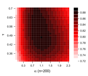
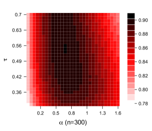
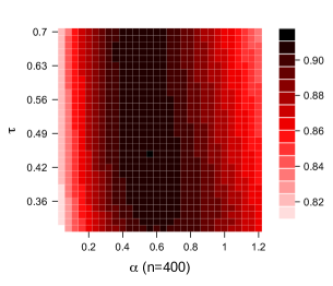
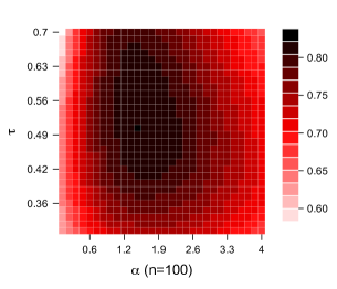
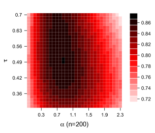
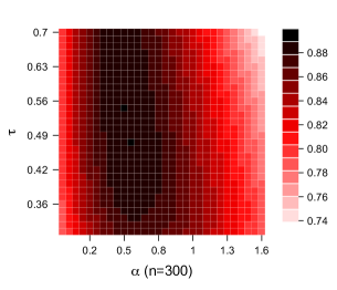
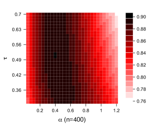
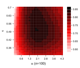
Figure 1 demonstrates the joint impact of the tuning parameters on the SDP performance under Scenario (A). First of all, the comparison of NMI between γn=0subscript𝛾𝑛0\gamma_{n}=0 and γn>0subscript𝛾𝑛0\gamma_{n}>0 indicates the effectiveness of SDP (10) for leveraging nodal information. We can also see that neither small or large values of γnsubscript𝛾𝑛\gamma_{n} lead to optimal performances, verifying the point we discussed in Section 4.1 that γnsubscript𝛾𝑛\gamma_{n} plays the role of balancing the edge and nodal information. An appropriate choice, as suggested by the four plots, is γn=[log(n)]0.5nsubscript𝛾𝑛superscriptdelimited-[]𝑛0.5𝑛\gamma_{n}=\frac{[\log(n)]^{0.5}}{n}, which is consistent with the result of Theorem 4. Regarding the parameter λnsubscript𝜆𝑛\lambda_{n}, we know from Theorem 4 that λn=n22subscript𝜆𝑛superscript𝑛22\lambda_{n}=\frac{n^{2}}{2} is the desired choice. Interestingly, Figure 1 shows that a wide range of λnsubscript𝜆𝑛\lambda_{n} can give competitive results, as long as the corresponding γnsubscript𝛾𝑛\gamma_{n} is properly chosen. For Scenario (B), similar phenomena can be observed in Figure 2. Note that since the nodal covariates are not as informative as in Scenario (A), the optimal γn0.8[log(n)]0.5nsubscript𝛾𝑛0.8superscriptdelimited-[]𝑛0.5𝑛\gamma_{n}\approx\frac{0.8[\log(n)]^{0.5}}{n} tends to give more weights to the adjacency matrix. The results in these two different settings confirm the implication of Theorem 4, that SDP (10) can work beyond NSBM.
Refer to caption Refer to caption
Figure 1: The community detection performance of SDP (measured by NMI), under Scenario (A), with different tuning parameters (λn,γn)subscript𝜆𝑛subscript𝛾𝑛(\lambda_{n},\gamma_{n}); NMI is averaged over 500 repetitions; We have used the scaled version of the tuning parameters: τ=λnn2,α=100γnformulae-sequence𝜏subscript𝜆𝑛superscript𝑛2𝛼100subscript𝛾𝑛\tau=\frac{\lambda_{n}}{n^{2}},\alpha=100\gamma_{n}.
Refer to caption Refer to caption
Figure 2: The community detection performance of SDP (measured by NMI), under Scenario (B), with different tuning parameters (λn,γn)subscript𝜆𝑛subscript𝛾𝑛(\lambda_{n},\gamma_{n}); NMI is averaged over 500 repetitions; We have used the scaled version of the tuning parameters: τ=λnn2,α=100γnformulae-sequence𝜏subscript𝜆𝑛superscript𝑛2𝛼100subscript𝛾𝑛\tau=\frac{\lambda_{n}}{n^{2}},\alpha=100\gamma_{n}.

5.1.2 Community Detection Performance via Variational and Maximum Profile Likelihood Methods.

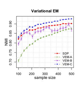
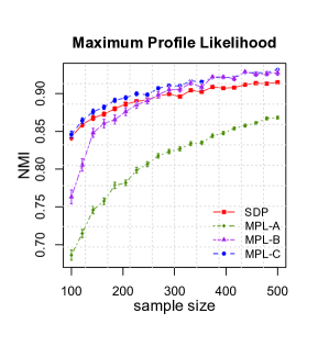
We implement variational and maximum profile likelihood methods via Algorithms 2 and 3 respectively, taking the outputs from Algorithm 1 as initialization (called VEM-C and MPL-C respectively). We do not predefine the number of iterations 𝒯𝒯\mathcal{T} in both algorithms, and instead keep iterating until convergence. To investigate the impact of SDP as an initialization, we have additionally implemented both methods with random initialization (called VEM-B and MPL-B respectively): run Algorithms 2 and 3 with random initialization independently multiple times and choose the outputs that give the largest objective function value (e.g., the profile likelihood function). We have also applied both methods for the simulated datasets with nodal attributes removed (called VEM-A and MPL-A respectively). This will be used as a comparison to check the effect of the two methods in incorporating nodal information. We set λn=12n2,γn=[log(n)]0.5nformulae-sequencesubscript𝜆𝑛12superscript𝑛2subscript𝛾𝑛superscriptdelimited-[]𝑛0.5𝑛\lambda_{n}=\frac{1}{2}n^{2},\gamma_{n}=\frac{[\log(n)]^{0.5}}{n} for all the implementations of SDP under Scenario (A); and λn=12n2,γn=0.8[log(n)]0.5nformulae-sequencesubscript𝜆𝑛12superscript𝑛2subscript𝛾𝑛0.8superscriptdelimited-[]𝑛0.5𝑛\lambda_{n}=\frac{1}{2}n^{2},\gamma_{n}=\frac{0.8[\log(n)]^{0.5}}{n} under Scenario (B).

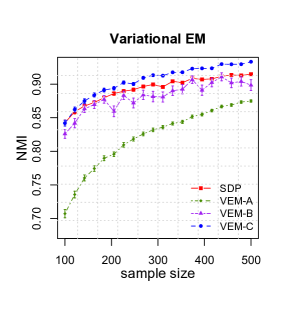
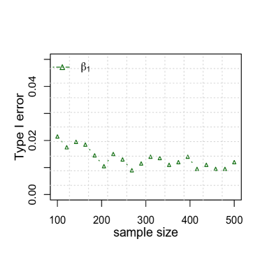
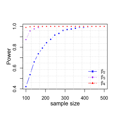
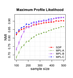
Figure 3 shows the community detection results of both methods under Scenario (A). By comparing the four curves in each plot, we can make a list of interesting observations: (1) SDP is a good initialization (MPL-C vs. MPL-B, VEM-C vs. VEM-B); (2) SDP itself already gives reasonable outputs, but the follow-up iterations further improve the performance (SDP vs.. MPL-C, SDP vs. VEM-C); (3) the nodal covariates are helpful for detecting communities, and the two methods have made effective use of it (MPL-A vs. MPL-C, VEM-A vs. VEM-C); (4) the two methods have similar performances when initialized with SDP (MPL-A vs. VEM-A, MPL-C vs. VEM-C). Moreover, we would like to point out the different behavior of the two methods with random initialization. The comparison between the two purple curves (MPL-B vs. VEM-B) implies that compared to the variational method, maximum profile likelihood method has the potential of exploring the parameter space more efficiently, especially when the sample size is large. One possible explanation is that the update of the “soft” community labels (the distribution {qik}subscript𝑞𝑖𝑘\{q_{ik}\}) in the variational algorithm may cause it to move very slowly in the parameter space and hence it may take many steps to change a label assignment. Furthermore, note that we can use the asymptotic normality property of the estimators for 𝜷𝜷\bm{\beta} in Theorems 2 and 3 to perform variable selection. The results of the Wald test regarding each component of 𝜷𝜷\bm{\beta} are presented in Figure 4. We see that our methods are able to identify relevant (the last three) and irrelevant (the first) nodal variables. Regarding Scenario (B), similar observations on the community detection performance can be made from Figure 6. We thus omit the details. As a final remark, the performances in Scenario (B) indicate that both methods can work to a certain extent of model misspecification.
Refer to caption Refer to caption
Figure 3: The community detection performances under Scenario (A); The average NMI is calculated over 500 repetitions along with its standard error bar; MPL-A, MPL-B and MPL-C represent the maximum profile likelihood methods with no nodal covariates being used, random initialization, and initialization from SDP, respectively; Similar notations are used for variational method. We have used 15 independent random initializations for maximum profile likelihood method across all the sample size; For variational method, the number of random initializations used starts from 15 for n=100𝑛100n=100 and consecutively increases by 1 for the subsequent sample sizes.
Refer to caption Refer to caption
Figure 4: Wald test for each component of β𝛽\beta. The calculations are averaged over 2000 repetitions. The significance level is set to 0.01. Since both variational and maximum profile likelihood methods give similar results, we only present the result of variational method for simplicity.
Refer to caption
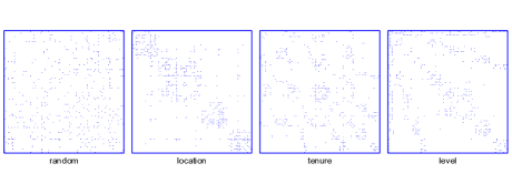
Figure 5: From left to right are the re-ordered adjacency matrices based on random permutation, location, tenure, and organizational level.
Refer to caption Refer to caption
Figure 6: The community detection performances under Scenario (B); All the relevant descriptions are the same as in Figure 3.

5.2 Real Data Analysis.

The dataset is about a research team consisting of 77 employees in a manufacturing company (Cross and Parker, 2004). A weight wijsubscript𝑤𝑖𝑗w_{ij} is assigned to the edge from employee i𝑖i to employee j𝑗j based on the extent to which employee i𝑖i provides employee j𝑗j with information j𝑗j uses to accomplish j𝑗j’s work. There are seven choices for the weights: 0 (I do not know this person/I have never met this person); 1 (Very infrequently); 2 (Infrequently); 3 (Somewhat infrequently); 4 (Somewhat frequently); 5 (Frequently); 6 (Very frequently). In addition to the edge information, the dataset also contains several attributes of each employee: location (1: Paris, 2: Frankfurt, 3: Warsaw, 4: Geneva); tenure (1: 1-12 months, 2: 13-36 months, 3: 37-60 months, 4: 61+ months); the organizational level (1: Global Dept Manager, 2: Local Dept Manager, 3: Project Leader, 4: Researcher). Since the network is a weighted and directed network, we first convert it to a binary network such that there exists an edge from i𝑖i to j𝑗j if and only if wij>3subscript𝑤𝑖𝑗3w_{ij}>3. This corresponds to whether the information is provided frequently or not. We then further convert it into an undirected network in the way that the edge between i𝑖i and j𝑗j exists if and only if both directed edges from i𝑖i to j𝑗j and j𝑗j to i𝑖i are present. Finally, we remove three isolated nodes from the network. To explore the intro-organizational community structure, we re-order the adjacency matrix based on random permutation and the attributes. As can be seen from Figure 5, the attribute “location” is a very informative indicator of the network’s community structure. This should not come as a big surprise, since the same office location usually promotes communication and collaboration between team members. We now use the “location” as the ground truth for the community assignment and examine the performances of SDP (10), maximum profile likelihood and variational methods based on the rest of the data. For SDP (10), we first use spectral clustering on adjacency matrix (Lei and Rinaldo, 2014) to estimate the size of the communities and plug the estimates in the formula of λnsubscript𝜆𝑛\lambda_{n} in Theorem 4 to determine λnsubscript𝜆𝑛\lambda_{n}. Regarding γnsubscript𝛾𝑛\gamma_{n}, motivated from the simulation results, we choose γn=ρ^nlognsubscript𝛾𝑛subscript^𝜌𝑛𝑛\gamma_{n}=\frac{\hat{\rho}_{n}}{\log n}, where ρ^n=2×number of edgesn2subscript^𝜌𝑛2number of edgessuperscript𝑛2\hat{\rho}_{n}=\frac{2\times\mbox{number of edges}}{n^{2}}. The maximum profile likelihood and variational methods are initialized by the output from SDP. We can see from Table 1 that by incorporating the nodal information, community detection accuracy has been improved. It is interesting to observe that SDP performs as well as the two likelihood based methods, when nodal covariates are available. Note that we can calculate the mutual information between the “ground truth” variable “location” and the other two to see how much community information they contain. Given that both mutual information (0.11 & 0.03) are pretty small, the magnitude of improvement in Table 1 is reasonable.

SDP MPL VEM SDP MPL VEM
edge 0.881 0.894 0.894 0.882 0.883 0.883
edge + nodal 0.920 0.920 0.920 0.921 0.921 0.921
Table 1: The community detection results of SDP, maximum profile likelihood, and variational methods. MPL and VEM denote maximum profile likelihood and variational methods, respectively. NMI is computed on the left part of the table, and ARI on the right. The row indexed by “edge” shows the results based on the network without nodal information, while the other one “edge+nodal” contains the results of making use of the two attributes available.

6 Discussion.

In this paper, we present a systematic study of the community detection with nodal information problem. We propose a flexible network modeling framework, and analyze three likelihood based methods under a specialized model. Both asymptotic and algorithmic aspects have been thoroughly discussed. The superiority of variational and maximum profile likelihood methods are verified through a variety of numerical experiments. Finally, we would like to highlight several potential extensions and open problems for future work.

  • 1.

    The modeling of both the network and nodal covariates can be readily extended to more general families, such as degree-corrected stochastic block model and non-parametric regression, respectively. The corresponding asymptotic results might be derived accordingly.

  • 2.

    In the setting with high dimensional covariates, penalized likelihood methods are more appealing for both community detection and variable selection. Theoretical analysis of community detection and variable selection consistency will be necessary.

  • 3.

    For very sparse networks, considering nρn=O(1)𝑛subscript𝜌𝑛𝑂1n\rho_{n}=O(1) seems to be a more realistic asymptotic framework. Under such asymptotic setting, community detection consistency is impossible. The effect of nodal covariates becomes more critical. It is of great interest to characterize the impact of the nodal information on community detection.

  • 4.

    In this work, we assume the number of communities K𝐾K is known. How to select K𝐾K is an important problem in community detection. Some recent efforts towards this direction include Saldana et al. (2015); Le and Levina (2015); Wang and Bickel (2015); Lei (2016).

Appendix A Appendix

Notations and Preliminaries. Before the proofs, we first introduce some necessary notations. Let πa=P(c=a),π^a=1ni=1n𝟙(ci=a),1aKformulae-sequencesubscript𝜋𝑎𝑃𝑐𝑎formulae-sequencesubscript^𝜋𝑎1𝑛superscriptsubscript𝑖1𝑛1subscript𝑐𝑖𝑎1𝑎𝐾\pi_{a}=P(c=a),\hat{\pi}_{a}=\frac{1}{n}\sum_{i=1}^{n}\mathbbm{1}(c_{i}=a),1\leq a\leq K. Given a community assignment 𝒆{1,,K}n𝒆superscript1𝐾𝑛\bm{e}\in\{1,\dots,K\}^{n}, define O(𝒆),V(𝒆),T(𝒆),T^(𝒆)K×K𝑂𝒆𝑉𝒆𝑇𝒆^𝑇𝒆superscript𝐾𝐾O(\bm{e}),V(\bm{e}),T(\bm{e}),\hat{T}(\bm{e})\in\mathbb{R}^{K\times K} and 𝒇0(𝒆),𝒇^(𝒆)Ksuperscript𝒇0𝒆^𝒇𝒆superscript𝐾\bm{f}^{0}(\bm{e}),\hat{\bm{f}}(\bm{e})\in\mathbb{R}^{K} with their elements being

Oab(𝒆)=ijAij𝟙(ei=a,ej=b),Vab(𝒆)=i𝟙(ei=a,ci=b)i𝟙(ci=b),formulae-sequencesubscript𝑂𝑎𝑏𝒆subscript𝑖𝑗subscript𝐴𝑖𝑗1formulae-sequencesubscript𝑒𝑖𝑎subscript𝑒𝑗𝑏subscript𝑉𝑎𝑏𝒆subscript𝑖1formulae-sequencesubscript𝑒𝑖𝑎subscript𝑐𝑖𝑏subscript𝑖1subscript𝑐𝑖𝑏\displaystyle O_{ab}(\bm{e})=\sum_{ij}A_{ij}\mathbbm{1}(e_{i}=a,e_{j}=b),\quad V_{ab}(\bm{e})=\frac{\sum_{i}\mathbbm{1}(e_{i}=a,c_{i}=b)}{\sum_{i}\mathbbm{1}(c_{i}=b)},
Tkl(𝒆)=abπaπbB¯abVka(𝒆)Vlb(𝒆),T^kl(𝒆)=abπ^aπ^bB¯abVka(𝒆)Vlb(𝒆),formulae-sequencesubscript𝑇𝑘𝑙𝒆subscript𝑎𝑏subscript𝜋𝑎subscript𝜋𝑏subscript¯𝐵𝑎𝑏subscript𝑉𝑘𝑎𝒆subscript𝑉𝑙𝑏𝒆subscript^𝑇𝑘𝑙𝒆subscript𝑎𝑏subscript^𝜋𝑎subscript^𝜋𝑏subscript¯𝐵𝑎𝑏subscript𝑉𝑘𝑎𝒆subscript𝑉𝑙𝑏𝒆\displaystyle T_{kl}(\bm{e})=\sum_{ab}\pi_{a}\pi_{b}\bar{B}_{ab}V_{ka}(\bm{e})V_{lb}(\bm{e}),\quad\hat{T}_{kl}(\bm{e})=\sum_{ab}\hat{\pi}_{a}\hat{\pi}_{b}\bar{B}_{ab}V_{ka}(\bm{e})V_{lb}(\bm{e}),
fk0(𝒆)=aVka(𝒆)πa,f^k(𝒆)=aVka(𝒆)π^a=nk(𝒆)n.formulae-sequencesubscriptsuperscript𝑓0𝑘𝒆subscript𝑎subscript𝑉𝑘𝑎𝒆subscript𝜋𝑎subscript^𝑓𝑘𝒆subscript𝑎subscript𝑉𝑘𝑎𝒆subscript^𝜋𝑎subscript𝑛𝑘𝒆𝑛\displaystyle f^{0}_{k}(\bm{e})=\sum_{a}V_{ka}(\bm{e})\pi_{a},\quad\hat{f}_{k}(\bm{e})=\sum_{a}V_{ka}(\bm{e})\hat{\pi}_{a}=\frac{n_{k}(\bm{e})}{n}.

Here, Oab(𝒆)subscript𝑂𝑎𝑏𝒆O_{ab}(\bm{e}) represents the number of edges between communities a𝑎a and b𝑏b under assignment 𝒆𝒆\bm{e} (twice the number when a=b𝑎𝑏a=b), Vab(𝒆)subscript𝑉𝑎𝑏𝒆V_{ab}(\bm{e}) represents the proportion of the nodes in community b𝑏b under 𝒄𝒄\bm{c} that are mislabeled as community a𝑎a under 𝒆𝒆\bm{e}, Tkl(𝒆)subscript𝑇𝑘𝑙𝒆T_{kl}(\bm{e}) reflects the connection probability (up to a scaling factor ρnsubscript𝜌𝑛\rho_{n}) between a node in community k𝑘k and another node in community l𝑙l under 𝒆𝒆\bm{e} with T^kl(𝒆)subscript^𝑇𝑘𝑙𝒆\hat{T}_{kl}(\bm{e}) being its empirical version, and f^k(𝒆)subscript^𝑓𝑘𝒆\hat{f}_{k}(\bm{e}) represents the proportion of community k𝑘k under 𝒆𝒆\bm{e} with fk0(𝒆)subscriptsuperscript𝑓0𝑘𝒆f^{0}_{k}(\bm{e}) as its “population” version. Also denote na(𝒆)=i𝟙(ei=a),1aK;F(T,𝒇)=ab(TablogTabfafbTab);(T,𝒇)=ab(TablogB¯abfafbB¯ab);𝒱={VK×K:kVka=1,Vka0,1k,aK};μn=n2ρnformulae-sequenceformulae-sequencesubscript𝑛𝑎𝒆subscript𝑖1subscript𝑒𝑖𝑎1𝑎𝐾formulae-sequence𝐹𝑇𝒇subscript𝑎𝑏subscript𝑇𝑎𝑏subscript𝑇𝑎𝑏subscript𝑓𝑎subscript𝑓𝑏subscript𝑇𝑎𝑏formulae-sequence𝑇𝒇subscript𝑎𝑏subscript𝑇𝑎𝑏subscript¯𝐵𝑎𝑏subscript𝑓𝑎subscript𝑓𝑏subscript¯𝐵𝑎𝑏formulae-sequence𝒱conditional-set𝑉superscript𝐾𝐾formulae-sequencesubscript𝑘subscript𝑉𝑘𝑎1formulae-sequencesubscript𝑉𝑘𝑎0formulae-sequence1𝑘𝑎𝐾subscript𝜇𝑛superscript𝑛2subscript𝜌𝑛n_{a}(\bm{e})=\sum_{i}\mathbbm{1}(e_{i}=a),1\leq a\leq K;F(T,\bm{f})=\sum_{ab}\Big{(}T_{ab}\log\frac{T_{ab}}{f_{a}f_{b}}-T_{ab}\Big{)};\mathcal{H}(T,\bm{f})=\sum_{ab}\Big{(}T_{ab}\log\bar{B}_{ab}-f_{a}f_{b}\bar{B}_{ab}\Big{)};\mathcal{V}=\{V\in\mathbb{R}^{K\times K}:\sum_{k}V_{ka}=1,V_{ka}\geq 0,1\leq k,a\leq K\};\mu_{n}=n^{2}\rho_{n}. Throughout the proofs, we use B0superscript𝐵0B^{0} and 𝜷0subscript𝜷0\bm{\beta}_{0} to represent the true parameters in NSBM while leaving B𝐵B and 𝜷𝜷\bm{\beta} as the generic parameter. We will C1subscript𝐶1C_{1}, C2subscript𝐶2C_{2}, \dots, to represent positive generic constants whose values may vary across different lines. We will frequently use the notation V(𝒆)V(𝒄)1=ab|Vab(𝒆)Vab(𝒄)|subscriptnorm𝑉𝒆𝑉𝒄1subscript𝑎𝑏subscript𝑉𝑎𝑏𝒆subscript𝑉𝑎𝑏𝒄\|V(\bm{e})-V(\bm{c})\|_{1}=\sum_{ab}|V_{ab}(\bm{e})-V_{ab}(\bm{c})|. Note that 1ni𝟙(eici)12V(𝒆)V(𝒄)11𝑛subscript𝑖1subscript𝑒𝑖subscript𝑐𝑖12subscriptnorm𝑉𝒆𝑉𝒄1\frac{1}{n}\sum_{i}\mathbbm{1}(e_{i}\neq c_{i})\leq\frac{1}{2}\|V(\bm{e})-V(\bm{c})\|_{1} (see the derivation on Page 22 of Zhao et al. (2012)). Moreover, we cite two concentration inequality results that will be used in the proof. The first one is Lemma A.1 from Zhao et al. (2012):

P(max𝒆maxab|Oab(𝒆)μnT^ab(𝒆)|ϵ)2Kn+2exp(ϵ2μn8maxabB¯ab),𝑃subscript𝒆subscript𝑎𝑏subscript𝑂𝑎𝑏𝒆subscript𝜇𝑛subscript^𝑇𝑎𝑏𝒆italic-ϵ2superscript𝐾𝑛2superscriptitalic-ϵ2subscript𝜇𝑛8subscript𝑎𝑏subscript¯𝐵𝑎𝑏\displaystyle P\Big{(}\max_{\bm{e}}\max_{ab}\Big{|}\frac{O_{ab}(\bm{e})}{\mu_{n}}-\hat{T}_{ab}(\bm{e})\Big{|}\geq\epsilon\Big{)}\leq 2K^{n+2}\exp({-\frac{\epsilon^{2}\mu_{n}}{8\max_{ab}\bar{B}_{ab}}}), (22)

for ϵ<3maxabB¯abitalic-ϵ3subscript𝑎𝑏subscript¯𝐵𝑎𝑏\epsilon<3\max_{ab}\bar{B}_{ab}. The second one is (1.4) in Bickel et al. (2015): γ0>0,for-allsubscript𝛾00\forall~{}\gamma_{0}>0,

P(max0<V(𝒆)V(𝒄)1δn[maxab|Xab(𝒆)Xab(𝒄)|γ0V(𝒆)V(𝒄)1]0)1,𝑃subscript0subscriptnorm𝑉𝒆𝑉𝒄1subscript𝛿𝑛subscript𝑎𝑏subscript𝑋𝑎𝑏𝒆subscript𝑋𝑎𝑏𝒄subscript𝛾0subscriptnorm𝑉𝒆𝑉𝒄101\displaystyle P\Big{(}\max_{0<\|V(\bm{e})-V(\bm{c})\|_{1}\leq\delta_{n}}[\max_{ab}|X_{ab}(\bm{e})-X_{ab}(\bm{c})|-\gamma_{0}\cdot\|V(\bm{e})-V(\bm{c})\|_{1}]\leq 0\Big{)}\rightarrow 1, (23)

where Xab(𝒆)=Oab(𝒆)μnT^ab(𝒆)subscript𝑋𝑎𝑏𝒆subscript𝑂𝑎𝑏𝒆subscript𝜇𝑛subscript^𝑇𝑎𝑏𝒆X_{ab}(\bm{e})=\frac{O_{ab}(\bm{e})}{\mu_{n}}-\hat{T}_{ab}(\bm{e}) and δn0,nρn/lognformulae-sequencesubscript𝛿𝑛0𝑛subscript𝜌𝑛𝑛\delta_{n}\rightarrow 0,n\rho_{n}/\log n\rightarrow\infty. Finally, we should be aware that the expressions involving community assignment 𝒆𝒆\bm{e} in the proofs are to be interpreted, up to permutations of community labels in {1,2,,K}12𝐾\{1,2,\dots,K\} whenever necessary.

Lemma 1.

There exist positive constants c0,c1,c2,c3>0subscript𝑐0subscript𝑐1subscript𝑐2subscript𝑐30c_{0},c_{1},c_{2},c_{3}>0, such that

F(T(c),f0(c))F(T(e),f0(e))c0V(e)V(c)1, if V(e)V(c)1c1,formulae-sequence𝐹𝑇csuperscriptf0c𝐹𝑇esuperscriptf0esubscript𝑐0subscriptnorm𝑉e𝑉c1 if subscriptnorm𝑉e𝑉c1subscript𝑐1\displaystyle F(T(\textbf{c}),\textbf{f}^{0}(\textbf{c}))-F(T(\textbf{e}),\textbf{f}^{0}(\textbf{e}))\geq c_{0}\cdot\|V(\textbf{e})-V(\textbf{c})\|_{1},\mbox{~{}~{}~{}if~{}}\|V(\textbf{e})-V(\textbf{c})\|_{1}\leq c_{1},
(T(c),f0(c))(T(e),f0(e))c2V(e)V(c)1, if V(e)V(c)1c3.formulae-sequence𝑇csuperscriptf0c𝑇esuperscriptf0esubscript𝑐2subscriptnorm𝑉e𝑉c1 if subscriptnorm𝑉e𝑉c1subscript𝑐3\displaystyle\mathcal{H}(T(\textbf{c}),\textbf{f}^{0}(\textbf{c}))-\mathcal{H}(T(\textbf{e}),\textbf{f}^{0}(\textbf{e}))\geq c_{2}\cdot\|V(\textbf{e})-V(\textbf{c})\|_{1},\mbox{~{}~{}~{}if~{}}\|V(\textbf{e})-V(\textbf{c})\|_{1}\leq c_{3}.
Proof.

We only show the proof for the first inequality since the second one can be derived in a similar way. Note that F(T(e),f0(e))𝐹𝑇esuperscriptf0eF(T(\textbf{e}),\textbf{f}^{0}(\textbf{e})) can be considered as a function of V(e)𝑉eV(\textbf{e}). We give it another notation H(V(e))𝐻𝑉eH(V(\textbf{e})), where H()𝐻H(\cdot) is defined on the convex set 𝒱𝒱\mathcal{V}. Further define g(ϵ;V(e))=H((1ϵ)V(c)+ϵV(e))𝑔italic-ϵ𝑉e𝐻1italic-ϵ𝑉citalic-ϵ𝑉eg(\epsilon;V(\textbf{e}))=H((1-\epsilon)V(\textbf{c})+\epsilon V(\textbf{e})), for 0ϵ10italic-ϵ10\leq\epsilon\leq 1. Since V(𝒆),V(𝒄)𝒱𝑉𝒆𝑉𝒄𝒱V(\bm{e}),V(\bm{c})\in\mathcal{V}, g(ϵ;V(e))𝑔italic-ϵ𝑉eg(\epsilon;V(\textbf{e})) is well defined. We first show that c~0,c~1>0subscript~𝑐0subscript~𝑐10\exists~{}\tilde{c}_{0},\tilde{c}_{1}>0, s.t.

g(ϵ;V(e))c~0V(e)V(c)1, for any 0ϵc~1,V(e)𝒱formulae-sequenceformulae-sequencesuperscript𝑔italic-ϵ𝑉esubscript~𝑐0subscriptnorm𝑉e𝑉c1 for any 0italic-ϵsubscript~𝑐1𝑉e𝒱\displaystyle g^{\prime}(\epsilon;V(\textbf{e}))\leq-\tilde{c}_{0}\cdot\|V(\textbf{e})-V(\textbf{c})\|_{1},\mbox{~{}for any~{}}0\leq\epsilon\leq\tilde{c}_{1},V(\textbf{e})\in\mathcal{V} (24)

where g(ϵ;V(e))superscript𝑔italic-ϵ𝑉eg^{\prime}(\epsilon;V(\textbf{e})) is the derivative with respect to ϵitalic-ϵ\epsilon; the constants c~0,c~1subscript~𝑐0subscript~𝑐1\tilde{c}_{0},\tilde{c}_{1} do not depend on V(e)𝑉eV(\textbf{e}). To prove (24), denote V~ka=(1ϵ)Vka(c)+ϵVka(e),rkl=abπaπbV~kaV~lbB¯ababπaπbV~kaV~lbformulae-sequencesubscript~𝑉𝑘𝑎1italic-ϵsubscript𝑉𝑘𝑎citalic-ϵsubscript𝑉𝑘𝑎esubscript𝑟𝑘𝑙subscript𝑎𝑏subscript𝜋𝑎subscript𝜋𝑏subscript~𝑉𝑘𝑎subscript~𝑉𝑙𝑏subscript¯𝐵𝑎𝑏subscript𝑎𝑏subscript𝜋𝑎subscript𝜋𝑏subscript~𝑉𝑘𝑎subscript~𝑉𝑙𝑏\tilde{V}_{ka}=(1-\epsilon)V_{ka}(\textbf{c})+\epsilon V_{ka}(\textbf{e}),r_{kl}=\frac{\sum_{ab}\pi_{a}\pi_{b}\tilde{V}_{ka}\tilde{V}_{lb}\bar{B}_{ab}}{\sum_{ab}\pi_{a}\pi_{b}\tilde{V}_{ka}\tilde{V}_{lb}}. Then a straightforward calculation gives us,

g(ϵ;V(e))=2ϵklabπaπb[Vka(e)Vka(c)][Vlb(e)Vlb(c)](B¯ablogrklrkl)superscript𝑔italic-ϵ𝑉e2italic-ϵsubscript𝑘𝑙subscript𝑎𝑏subscript𝜋𝑎subscript𝜋𝑏delimited-[]subscript𝑉𝑘𝑎esubscript𝑉𝑘𝑎cdelimited-[]subscript𝑉𝑙𝑏esubscript𝑉𝑙𝑏csubscript¯𝐵𝑎𝑏subscript𝑟𝑘𝑙subscript𝑟𝑘𝑙\displaystyle g^{\prime}(\epsilon;V(\textbf{e}))=2\epsilon\sum_{kl}\sum_{ab}\pi_{a}\pi_{b}\cdot[V_{ka}(\textbf{e})-V_{ka}(\textbf{c})]\cdot[V_{lb}(\textbf{e})-V_{lb}(\textbf{c})]\cdot(\bar{B}_{ab}\log r_{kl}-r_{kl}) (25)
+klabπaπb([Vka(e)Vka(c)]Vlb(c)+[Vlb(e)Vlb(c)]Vka(c))(B¯ablogrklrkl).subscript𝑘𝑙subscript𝑎𝑏subscript𝜋𝑎subscript𝜋𝑏delimited-[]subscript𝑉𝑘𝑎esubscript𝑉𝑘𝑎csubscript𝑉𝑙𝑏cdelimited-[]subscript𝑉𝑙𝑏esubscript𝑉𝑙𝑏csubscript𝑉𝑘𝑎csubscript¯𝐵𝑎𝑏subscript𝑟𝑘𝑙subscript𝑟𝑘𝑙\displaystyle+\sum_{kl}\sum_{ab}\pi_{a}\pi_{b}([V_{ka}(\textbf{e})-V_{ka}(\textbf{c})]V_{lb}(\textbf{c})+[V_{lb}(\textbf{e})-V_{lb}(\textbf{c})]V_{ka}(\textbf{c}))\cdot(\bar{B}_{ab}\log r_{kl}-r_{kl}).

Hence when ϵ=0italic-ϵ0\epsilon=0, the above equation can be simplified as

g(0;V(e))superscript𝑔0𝑉e\displaystyle g^{\prime}(0;V(\textbf{e})) =kalbπaπb[Vka(e)Vka(c)]Vlb(c)(B¯ablogB¯klB¯kl)absentsubscript𝑘𝑎subscript𝑙𝑏subscript𝜋𝑎subscript𝜋𝑏delimited-[]subscript𝑉𝑘𝑎esubscript𝑉𝑘𝑎csubscript𝑉𝑙𝑏csubscript¯𝐵𝑎𝑏subscript¯𝐵𝑘𝑙subscript¯𝐵𝑘𝑙\displaystyle=\sum_{ka}\sum_{lb}\pi_{a}\pi_{b}\cdot[V_{ka}(\textbf{e})-V_{ka}(\textbf{c})]\cdot V_{lb}(\textbf{c})\cdot(\bar{B}_{ab}\log\bar{B}_{kl}-\bar{B}_{kl}) (26)
+lbkaπaπb[Vlb(e)Vlb(c)]Vka(c)(B¯ablogB¯klB¯kl)subscript𝑙𝑏subscript𝑘𝑎subscript𝜋𝑎subscript𝜋𝑏delimited-[]subscript𝑉𝑙𝑏esubscript𝑉𝑙𝑏csubscript𝑉𝑘𝑎csubscript¯𝐵𝑎𝑏subscript¯𝐵𝑘𝑙subscript¯𝐵𝑘𝑙\displaystyle\quad+\sum_{lb}\sum_{ka}\pi_{a}\pi_{b}\cdot[V_{lb}(\textbf{e})-V_{lb}(\textbf{c})]\cdot V_{ka}(\textbf{c})\cdot(\bar{B}_{ab}\log\bar{B}_{kl}-\bar{B}_{kl})
=kabπaπb(Vka(e)Vka(c))(B¯ablogB¯kbB¯kb)absentsubscript𝑘𝑎subscript𝑏subscript𝜋𝑎subscript𝜋𝑏subscript𝑉𝑘𝑎esubscript𝑉𝑘𝑎csubscript¯𝐵𝑎𝑏subscript¯𝐵𝑘𝑏subscript¯𝐵𝑘𝑏\displaystyle=\sum_{ka}\sum_{b}\pi_{a}\pi_{b}\cdot(V_{ka}(\textbf{e})-V_{ka}(\textbf{c}))\cdot(\bar{B}_{ab}\log\bar{B}_{kb}-\bar{B}_{kb})
+lbaπaπb(Vlb(e)Vlb(c))(B¯ablogB¯alB¯al)subscript𝑙𝑏subscript𝑎subscript𝜋𝑎subscript𝜋𝑏subscript𝑉𝑙𝑏esubscript𝑉𝑙𝑏csubscript¯𝐵𝑎𝑏subscript¯𝐵𝑎𝑙subscript¯𝐵𝑎𝑙\displaystyle\quad+\sum_{lb}\sum_{a}\pi_{a}\pi_{b}\cdot(V_{lb}(\textbf{e})-V_{lb}(\textbf{c}))\cdot(\bar{B}_{ab}\log\bar{B}_{al}-\bar{B}_{al})
=2ablπaπb(Vlb(e)Vlb(c))(B¯ablogB¯alB¯al).absent2subscript𝑎𝑏𝑙subscript𝜋𝑎subscript𝜋𝑏subscript𝑉𝑙𝑏esubscript𝑉𝑙𝑏csubscript¯𝐵𝑎𝑏subscript¯𝐵𝑎𝑙subscript¯𝐵𝑎𝑙\displaystyle=2\sum_{abl}\pi_{a}\pi_{b}(V_{lb}(\textbf{e})-V_{lb}(\textbf{c}))\cdot(\bar{B}_{ab}\log\bar{B}_{al}-\bar{B}_{al}).

Note that for any V(e)𝒱𝑉e𝒱V(\textbf{e})\in\mathcal{V}, it holds that Vbb(e)1=lbVlb(e)subscript𝑉𝑏𝑏e1subscript𝑙𝑏subscript𝑉𝑙𝑏eV_{bb}(\textbf{e})-1=-\sum_{l\neq b}V_{lb}(\textbf{e}). We can then continue the calculation from (26):

g(0;V(e))superscript𝑔0𝑉e\displaystyle~{}g^{\prime}(0;V(\textbf{e})) (27)
=\displaystyle= 2ab[πaπb(Vbb(e)1)(B¯ablogB¯abB¯ab)+lbπaπbVlb(e)(B¯ablogB¯alB¯al)]2subscript𝑎𝑏delimited-[]subscript𝜋𝑎subscript𝜋𝑏subscript𝑉𝑏𝑏e1subscript¯𝐵𝑎𝑏subscript¯𝐵𝑎𝑏subscript¯𝐵𝑎𝑏subscript𝑙𝑏subscript𝜋𝑎subscript𝜋𝑏subscript𝑉𝑙𝑏esubscript¯𝐵𝑎𝑏subscript¯𝐵𝑎𝑙subscript¯𝐵𝑎𝑙\displaystyle~{}2\sum_{ab}\Big{[}\pi_{a}\pi_{b}\cdot(V_{bb}(\textbf{e})-1)\cdot(\bar{B}_{ab}\log\bar{B}_{ab}-\bar{B}_{ab})+\sum_{l\neq b}\pi_{a}\pi_{b}\cdot V_{lb}(\textbf{e})\cdot(\bar{B}_{ab}\log\bar{B}_{al}-\bar{B}_{al})\Big{]}
=\displaystyle= 2ablbπaπbVlb(e)[B¯ablogB¯alB¯alB¯ablogB¯ab+B¯ab]2subscript𝑎𝑏subscript𝑙𝑏subscript𝜋𝑎subscript𝜋𝑏subscript𝑉𝑙𝑏edelimited-[]subscript¯𝐵𝑎𝑏subscript¯𝐵𝑎𝑙subscript¯𝐵𝑎𝑙subscript¯𝐵𝑎𝑏subscript¯𝐵𝑎𝑏subscript¯𝐵𝑎𝑏\displaystyle~{}2\sum_{ab}\sum_{l\neq b}\pi_{a}\pi_{b}\cdot V_{lb}(\textbf{e})\cdot[\bar{B}_{ab}\log\bar{B}_{al}-\bar{B}_{al}-\bar{B}_{ab}\log\bar{B}_{ab}+\bar{B}_{ab}]
=(a)𝑎\displaystyle\overset{(a)}{=} 2ablbπaπbVlb(e)B¯ab(B¯alB¯ab)22B~ab2(b)c~2ablbVlb(e)(B¯alB¯ab)22subscript𝑎𝑏subscript𝑙𝑏subscript𝜋𝑎subscript𝜋𝑏subscript𝑉𝑙𝑏esubscript¯𝐵𝑎𝑏superscriptsubscript¯𝐵𝑎𝑙subscript¯𝐵𝑎𝑏22subscriptsuperscript~𝐵2𝑎𝑏𝑏subscript~𝑐2subscript𝑎𝑏subscript𝑙𝑏subscript𝑉𝑙𝑏esuperscriptsubscript¯𝐵𝑎𝑙subscript¯𝐵𝑎𝑏2\displaystyle~{}2\sum_{ab}\sum_{l\neq b}\pi_{a}\pi_{b}\cdot V_{lb}(\textbf{e})\cdot\frac{-\bar{B}_{ab}(\bar{B}_{al}-\bar{B}_{ab})^{2}}{2\tilde{B}^{2}_{ab}}\overset{(b)}{\leq}-\tilde{c}_{2}\cdot\sum_{ab}\sum_{l\neq b}V_{lb}(\textbf{e})\cdot(\bar{B}_{al}-\bar{B}_{ab})^{2}
=\displaystyle= c~2blb[Vlb(e)a(B¯alB¯ab)2](c)c~3blbVlb(e)=c~32V(e)V(c)1,subscript~𝑐2subscript𝑏subscript𝑙𝑏delimited-[]subscript𝑉𝑙𝑏esubscript𝑎superscriptsubscript¯𝐵𝑎𝑙subscript¯𝐵𝑎𝑏2𝑐subscript~𝑐3subscript𝑏subscript𝑙𝑏subscript𝑉𝑙𝑏esubscript~𝑐32subscriptnorm𝑉e𝑉c1\displaystyle~{}-\tilde{c}_{2}\cdot\sum_{b}\sum_{l\neq b}[V_{lb}(\textbf{e})\cdot\sum_{a}(\bar{B}_{al}-\bar{B}_{ab})^{2}]\overset{(c)}{\leq}-\tilde{c}_{3}\cdot\sum_{b}\sum_{l\neq b}V_{lb}(\textbf{e})=-\frac{\tilde{c}_{3}}{2}\|V(\textbf{e})-V(\textbf{c})\|_{1},

where B~absubscript~𝐵𝑎𝑏\tilde{B}_{ab} is a number between B¯absubscript¯𝐵𝑎𝑏\bar{B}_{ab} and B¯alsubscript¯𝐵𝑎𝑙\bar{B}_{al}. To obtain (a), we have used the second order Taylor expansion of the function B¯ablogxxsubscript¯𝐵𝑎𝑏𝑥𝑥\bar{B}_{ab}\log x-x around its maxima x=B¯ab𝑥subscript¯𝐵𝑎𝑏x=\bar{B}_{ab}; (b) is simply due to minaπa>0,minabB¯ab>0formulae-sequencesubscript𝑎subscript𝜋𝑎0subscript𝑎𝑏subscript¯𝐵𝑎𝑏0\min_{a}\pi_{a}>0,\min_{ab}\bar{B}_{ab}>0; (c) holds since B¯¯𝐵\bar{B} has no two identical columns. In order to obtain (24), we need to evaluate g(ϵ;V(e))superscript𝑔italic-ϵ𝑉eg^{\prime}(\epsilon;V(\textbf{e})) for small ϵitalic-ϵ\epsilon. From (25) and (26), it is straightforward to see

g(ϵ;V(e))g(0;V(e))superscript𝑔italic-ϵ𝑉esuperscript𝑔0𝑉e\displaystyle~{}g^{\prime}(\epsilon;V(\textbf{e}))-g^{\prime}(0;V(\textbf{e})) (28)
=\displaystyle= 2ϵklabπaπb[Vka(e)Vka(c)][Vlb(e)Vlb(c)](B¯ablogrklrkl)G1subscript2italic-ϵsubscript𝑘𝑙𝑎𝑏subscript𝜋𝑎subscript𝜋𝑏delimited-[]subscript𝑉𝑘𝑎esubscript𝑉𝑘𝑎cdelimited-[]subscript𝑉𝑙𝑏esubscript𝑉𝑙𝑏csubscript¯𝐵𝑎𝑏subscript𝑟𝑘𝑙subscript𝑟𝑘𝑙absentsubscript𝐺1\displaystyle~{}\underbrace{2\epsilon\cdot\sum_{klab}\pi_{a}\pi_{b}\cdot[V_{ka}(\textbf{e})-V_{ka}(\textbf{c})]\cdot[V_{lb}(\textbf{e})-V_{lb}(\textbf{c})]\cdot(\bar{B}_{ab}\log r_{kl}-r_{kl})}_{\triangleq G_{1}}
+klabπaπbB¯ab([Vka(e)Vka(c)]Vlb(c)+[Vlb(e)Vlb(c)]Vka(c))logrklB¯klG2subscriptsubscript𝑘𝑙𝑎𝑏subscript𝜋𝑎subscript𝜋𝑏subscript¯𝐵𝑎𝑏delimited-[]subscript𝑉𝑘𝑎esubscript𝑉𝑘𝑎csubscript𝑉𝑙𝑏cdelimited-[]subscript𝑉𝑙𝑏esubscript𝑉𝑙𝑏csubscript𝑉𝑘𝑎csubscript𝑟𝑘𝑙subscript¯𝐵𝑘𝑙absentsubscript𝐺2\displaystyle+\underbrace{\sum_{klab}\pi_{a}\pi_{b}\bar{B}_{ab}([V_{ka}(\textbf{e})-V_{ka}(\textbf{c})]V_{lb}(\textbf{c})+[V_{lb}(\textbf{e})-V_{lb}(\textbf{c})]V_{ka}(\textbf{c}))\cdot\log\frac{r_{kl}}{\bar{B}_{kl}}}_{\triangleq G_{2}}
klabπaπb([Vka(e)Vka(c)]Vlb(c)+[Vlb(e)Vlb(c)]Vka(c))(rklB¯kl)G3.subscriptsubscript𝑘𝑙𝑎𝑏subscript𝜋𝑎subscript𝜋𝑏delimited-[]subscript𝑉𝑘𝑎esubscript𝑉𝑘𝑎csubscript𝑉𝑙𝑏cdelimited-[]subscript𝑉𝑙𝑏esubscript𝑉𝑙𝑏csubscript𝑉𝑘𝑎csubscript𝑟𝑘𝑙subscript¯𝐵𝑘𝑙absentsubscript𝐺3\displaystyle-\underbrace{\sum_{klab}\pi_{a}\pi_{b}([V_{ka}(\textbf{e})-V_{ka}(\textbf{c})]V_{lb}(\textbf{c})+[V_{lb}(\textbf{e})-V_{lb}(\textbf{c})]V_{ka}(\textbf{c}))\cdot(r_{kl}-\bar{B}_{kl})}_{\triangleq G_{3}}.

We now bound G1,G2subscript𝐺1subscript𝐺2G_{1},G_{2} and G3subscript𝐺3G_{3} in the above equation. For G1subscript𝐺1G_{1}, note that |logrkl|maxab|logB¯ab|subscript𝑟𝑘𝑙subscript𝑎𝑏subscript¯𝐵𝑎𝑏|\log r_{kl}|\leq\max_{ab}|\log\bar{B}_{ab}| and |rkl|maxabB¯absubscript𝑟𝑘𝑙subscript𝑎𝑏subscript¯𝐵𝑎𝑏|r_{kl}|\leq\max_{ab}\bar{B}_{ab}. Therefore, c~4>0subscript~𝑐40\exists~{}\tilde{c}_{4}>0 such that

|G1|c~4ϵkabl|Vka(e)Vka(c)||Vlb(e)Vlb(c)|2K2c~4ϵV(e)V(c)1.subscript𝐺1subscript~𝑐4italic-ϵsubscript𝑘𝑎subscript𝑏𝑙subscript𝑉𝑘𝑎esubscript𝑉𝑘𝑎csubscript𝑉𝑙𝑏esubscript𝑉𝑙𝑏c2superscript𝐾2subscript~𝑐4italic-ϵsubscriptnorm𝑉e𝑉c1\displaystyle|G_{1}|\leq\tilde{c}_{4}\epsilon\cdot\sum_{ka}\sum_{bl}|V_{ka}(\textbf{e})-V_{ka}(\textbf{c})|\cdot|V_{lb}(\textbf{e})-V_{lb}(\textbf{c})|\leq 2K^{2}\tilde{c}_{4}\epsilon\cdot\|V(\textbf{e})-V(\textbf{c})\|_{1}. (29)

Regarding G2subscript𝐺2G_{2}, since V~kaVka(c)=O(ϵ)subscript~𝑉𝑘𝑎subscript𝑉𝑘𝑎c𝑂italic-ϵ\tilde{V}_{ka}-V_{ka}(\textbf{c})=O(\epsilon), we have

logrklB¯kl=logπkπlB¯kl+O(ϵ)πkπlB¯kl+O(ϵ)=O(ϵ).subscript𝑟𝑘𝑙subscript¯𝐵𝑘𝑙subscript𝜋𝑘subscript𝜋𝑙subscript¯𝐵𝑘𝑙𝑂italic-ϵsubscript𝜋𝑘subscript𝜋𝑙subscript¯𝐵𝑘𝑙𝑂italic-ϵ𝑂italic-ϵ\displaystyle\log\frac{r_{kl}}{\bar{B}_{kl}}=\log\frac{\pi_{k}\pi_{l}\bar{B}_{kl}+O(\epsilon)}{\pi_{k}\pi_{l}\bar{B}_{kl}+O(\epsilon)}=O(\epsilon).

So we can bound G2subscript𝐺2G_{2}:

|G2|O(ϵ)klab(|Vka(e)Vka(c)|+|Vlb(e)Vlb(c)|)=O(ϵ)V(e)V(c)1.subscript𝐺2𝑂italic-ϵsubscript𝑘𝑙𝑎𝑏subscript𝑉𝑘𝑎esubscript𝑉𝑘𝑎csubscript𝑉𝑙𝑏esubscript𝑉𝑙𝑏c𝑂italic-ϵsubscriptnorm𝑉e𝑉c1\displaystyle|G_{2}|\leq O(\epsilon)\cdot\sum_{klab}(|V_{ka}(\textbf{e})-V_{ka}(\textbf{c})|+|V_{lb}(\textbf{e})-V_{lb}(\textbf{c})|)=O(\epsilon)\cdot\|V(\textbf{e})-V(\textbf{c})\|_{1}. (30)

Similar arguments can give us |G3|=O(ϵ)V(e)V(c)1subscript𝐺3𝑂italic-ϵsubscriptnorm𝑉e𝑉c1|G_{3}|=O(\epsilon)\cdot\|V(\textbf{e})-V(\textbf{c})\|_{1}. This fact combined with (27), (28), (29) and (30) completes the proof of (24). We now consider any V(e)𝑉eV(\textbf{e}) such that V(e)V(c)1c~1subscriptnorm𝑉e𝑉c1subscript~𝑐1\|V(\textbf{e})-V(\textbf{c})\|_{1}\leq\tilde{c}_{1}. Define V(e)=V(c)+V(e)V(c)V(e)V(c)1superscript𝑉e𝑉c𝑉e𝑉csubscriptnorm𝑉e𝑉c1{V}^{*}(\textbf{e})=V(\textbf{c})+\frac{V(\textbf{e})-V(\textbf{c})}{\|V(\textbf{e})-V(\textbf{c})\|_{1}}. It is then straightforward to confirm that V(𝒆)𝒱superscript𝑉𝒆𝒱V^{*}(\bm{e})\in\mathcal{V}. Hence,

F(T(c),f0(c))F(T(e),f0(e))=H(V(c))H(V(e))𝐹𝑇csuperscriptf0c𝐹𝑇esuperscriptf0e𝐻𝑉c𝐻𝑉e\displaystyle F(T(\textbf{c}),\textbf{f}^{0}(\textbf{c}))-F(T(\textbf{e}),\textbf{f}^{0}(\textbf{e}))=H(V(\textbf{c}))-H(V(\textbf{e}))
=g(0;V(e))g(V(e)V(c)1;V(e))absent𝑔0superscript𝑉e𝑔subscriptnorm𝑉e𝑉c1superscript𝑉e\displaystyle=g(0;V^{*}(\textbf{e}))-g(\|V(\textbf{e})-V(\textbf{c})\|_{1};V^{*}(\textbf{e}))
=(d)g(ϵ~;V(e))V(e)V(c)1(e)c~0V(e)V(c)1V(e)V(c)1𝑑superscript𝑔~italic-ϵsuperscript𝑉esubscriptnorm𝑉e𝑉c1𝑒subscript~𝑐0subscriptnormsuperscript𝑉e𝑉c1subscriptnorm𝑉e𝑉c1\displaystyle\overset{(d)}{=}-g^{\prime}(\tilde{\epsilon};V^{*}(\textbf{e}))\cdot\|V(\textbf{e})-V(\textbf{c})\|_{1}\overset{(e)}{\geq}\tilde{c}_{0}\cdot\|V^{*}(\textbf{e})-V(\textbf{c})\|_{1}\cdot\|V(\textbf{e})-V(\textbf{c})\|_{1}
=c~0V(e)V(c)1,absentsubscript~𝑐0subscriptnorm𝑉e𝑉c1\displaystyle=\tilde{c}_{0}\cdot\|V(\textbf{e})-V(\textbf{c})\|_{1},

where (d) is simply by mean value theorem; ϵ~~italic-ϵ\tilde{\epsilon} is between 00 and V(eV(c))1subscriptnorm𝑉e𝑉c1\|V(\textbf{e}-V(\textbf{c}))\|_{1}; (e) holds because of (24). This finishes the proof. ∎

Proof of Theorem 1. It is not hard to check that similar proofs as the ones of Lemma 1 and Theorem 2 in Bickel et al. (2013) work under NSBM444The tail condition on 𝒙𝒙\bm{x} is used to show that Theorem 1 in Bickel et al. (2013) holds under NSBM.. For simplicity, we do not repeat the derivations here. As a result, we can obtain that as n𝑛n\rightarrow\infty,

n(𝜷^𝜷0)N(0,I1(𝜷0)),n2ρnlogB^abBab0=Op(1),1a,bK.formulae-sequence𝑛^𝜷subscript𝜷0𝑁0superscript𝐼1subscript𝜷0formulae-sequencesuperscript𝑛2subscript𝜌𝑛subscript^𝐵𝑎𝑏subscriptsuperscript𝐵0𝑎𝑏subscript𝑂𝑝1formulae-sequence1𝑎𝑏𝐾\displaystyle\sqrt{n}(\hat{\bm{\beta}}-\bm{\beta}_{0})\rightarrow N(0,I^{-1}(\bm{\beta}_{0})),\quad\sqrt{n^{2}\rho_{n}}\log\frac{\hat{B}_{ab}}{B^{0}_{ab}}=O_{p}(1),~{}~{}1\leq a,b\leq K. (31)

Based on (31), we would like to show the strong consistency of 𝒄^^𝒄\hat{\bm{c}}. Define

𝒩(𝒆;{Bab})𝒩𝒆subscript𝐵𝑎𝑏\displaystyle\mathcal{N}(\bm{e};\{B_{ab}\}) =ab[Oab(𝒆)μnlogBabρn+na(𝒆)nb(𝒆)Oab(𝒆)μnlog(1Bab)],absentsubscript𝑎𝑏delimited-[]subscript𝑂𝑎𝑏𝒆subscript𝜇𝑛subscript𝐵𝑎𝑏subscript𝜌𝑛subscript𝑛𝑎𝒆subscript𝑛𝑏𝒆subscript𝑂𝑎𝑏𝒆subscript𝜇𝑛1subscript𝐵𝑎𝑏\displaystyle=\sum_{ab}\Big{[}\frac{O_{ab}(\bm{e})}{\mu_{n}}\log\frac{B_{ab}}{\rho_{n}}+\frac{n_{a}(\bm{e})n_{b}(\bm{e})-O_{ab}(\bm{e})}{\mu_{n}}\log(1-B_{ab})\Big{]},
𝒞(𝒆;𝜷)𝒞𝒆𝜷\displaystyle\mathcal{C}(\bm{e};\bm{\beta}) =1μni[𝜷eiT𝒙ilog(k=1Kexp(𝜷kT𝒙i))].absent1subscript𝜇𝑛subscript𝑖delimited-[]subscriptsuperscript𝜷𝑇subscript𝑒𝑖subscript𝒙𝑖superscriptsubscript𝑘1𝐾subscriptsuperscript𝜷𝑇𝑘subscript𝒙𝑖\displaystyle=\frac{1}{\mu_{n}}\sum_{i}\Big{[}\bm{\beta}^{T}_{e_{i}}\bm{x}_{i}-\log\Big{(}\sum_{k=1}^{K}\exp({\bm{\beta}^{T}_{k}\bm{x}_{i}})\Big{)}\Big{]}.

We then easily see that

𝒄^=argmax𝒆{1,,K}n𝒩(𝒆;{B^ab})+𝒞(𝒆;𝜷^).^𝒄subscriptargmax𝒆superscript1𝐾𝑛𝒩𝒆subscript^𝐵𝑎𝑏𝒞𝒆^𝜷\displaystyle\hat{\bm{c}}=\operatorname*{arg\,max}_{\bm{e}\in\{1,\dots,K\}^{n}}\mathcal{N}(\bm{e};\{\hat{B}_{ab}\})+\mathcal{C}(\bm{e};\hat{\bm{\beta}}).

The subsequent proof is aligned with the ideas of proving strong consistency in Zhao et al. (2012). We first prove that 𝒄^^𝒄\hat{\bm{c}} is weak consistent. Note that

max𝒆|𝒩(e;{B^ab})(T(𝒆),𝒇0(𝒆))|subscript𝒆𝒩esubscript^𝐵𝑎𝑏𝑇𝒆superscript𝒇0𝒆\displaystyle\max_{\bm{e}}|\mathcal{N}(\textbf{e};\{\hat{B}_{ab}\})-\mathcal{H}(T(\bm{e}),\bm{f}^{0}(\bm{e}))| max𝒆|𝒩(e;{B^ab})𝒩(e;{Bab0})|absentsubscript𝒆𝒩esubscript^𝐵𝑎𝑏𝒩esubscriptsuperscript𝐵0𝑎𝑏\displaystyle\leq\max_{\bm{e}}|\mathcal{N}(\textbf{e};\{\hat{B}_{ab}\})-\mathcal{N}(\textbf{e};\{B^{0}_{ab}\})| (32)
+max𝒆|𝒩(𝒆;{Bab0})(T^(𝒆),𝒇^(𝒆))|subscript𝒆𝒩𝒆subscriptsuperscript𝐵0𝑎𝑏^𝑇𝒆^𝒇𝒆\displaystyle+\max_{\bm{e}}|\mathcal{N}(\bm{e};\{B^{0}_{ab}\})-\mathcal{H}(\hat{T}(\bm{e}),\hat{\bm{f}}(\bm{e}))|
+max𝒆|(T^(𝒆),𝒇^(𝒆))(T(𝒆),𝒇0(𝒆))|.subscript𝒆^𝑇𝒆^𝒇𝒆𝑇𝒆superscript𝒇0𝒆\displaystyle+\max_{\bm{e}}|\mathcal{H}(\hat{T}(\bm{e}),\hat{\bm{f}}(\bm{e}))-\mathcal{H}(T(\bm{e}),\bm{f}^{0}(\bm{e}))|.

We aim to bound the three terms on the right hand side of the above inequality. For the first one, we have

max𝒆|𝒩(e;{B^ab})𝒩(e;{Bab0})|subscript𝒆𝒩esubscript^𝐵𝑎𝑏𝒩esubscriptsuperscript𝐵0𝑎𝑏absent\displaystyle\max_{\bm{e}}|\mathcal{N}(\textbf{e};\{\hat{B}_{ab}\})-\mathcal{N}(\textbf{e};\{B^{0}_{ab}\})|\leq ab[max𝒆Oab(𝒆)μn|logB^ab(1Bab0)Bab0(1B^ab)|\displaystyle\sum_{ab}\Bigg{[}\max_{\bm{e}}\frac{O_{ab}(\bm{e})}{\mu_{n}}\cdot\Big{|}\log\frac{\hat{B}_{ab}(1-B^{0}_{ab})}{B^{0}_{ab}(1-\hat{B}_{ab})}\Big{|}
+1ρn|log1B^ab1Bab0|].\displaystyle+\frac{1}{\rho_{n}}\Big{|}\log\frac{1-\hat{B}_{ab}}{1-B^{0}_{ab}}\Big{|}\Bigg{]}.

According to (31), if we can show max𝒆Oab(𝒆)μn=Op(1)subscript𝒆subscript𝑂𝑎𝑏𝒆subscript𝜇𝑛subscript𝑂𝑝1\max_{\bm{e}}\frac{O_{ab}(\bm{e})}{\mu_{n}}=O_{p}(1), the above inequality will imply an0subscript𝑎𝑛0\exists~{}a_{n}\rightarrow 0 s.t.

P(max𝒆|𝒩(e;{B^ab})𝒩(e;{Bab0})|an)1.𝑃subscript𝒆𝒩esubscript^𝐵𝑎𝑏𝒩esubscriptsuperscript𝐵0𝑎𝑏subscript𝑎𝑛1\displaystyle P(\max_{\bm{e}}|\mathcal{N}(\textbf{e};\{\hat{B}_{ab}\})-\mathcal{N}(\textbf{e};\{B^{0}_{ab}\})|\leq a_{n})\rightarrow 1. (33)

For that purpose, we first apply (22) by choosing ϵn=(nρn)1/3subscriptitalic-ϵ𝑛superscript𝑛subscript𝜌𝑛13\epsilon_{n}=(n\rho_{n})^{-1/3} to have

P(max𝒆maxkl|Okl(𝒆)μnT^kl(𝒆)|ϵn)1.𝑃subscript𝒆subscript𝑘𝑙subscript𝑂𝑘𝑙𝒆subscript𝜇𝑛subscript^𝑇𝑘𝑙𝒆subscriptitalic-ϵ𝑛1\displaystyle P\Big{(}\max_{\bm{e}}\max_{kl}\Big{|}\frac{O_{kl}(\bm{e})}{\mu_{n}}-\hat{T}_{kl}(\bm{e})\Big{|}\leq\epsilon_{n}\Big{)}\rightarrow 1. (34)

Also notice that max𝒆|Tkl(𝒆)|abB¯absubscript𝒆subscript𝑇𝑘𝑙𝒆subscript𝑎𝑏subscript¯𝐵𝑎𝑏\max_{\bm{e}}|T_{kl}(\bm{e})|\leq\sum_{ab}\bar{B}_{ab}, and

max𝒆|Tkl(𝒆)T^kl(𝒆)|abB¯ab(|π^aπa|+|π^bπb|)𝑃0.subscript𝒆subscript𝑇𝑘𝑙𝒆subscript^𝑇𝑘𝑙𝒆subscript𝑎𝑏subscript¯𝐵𝑎𝑏subscript^𝜋𝑎subscript𝜋𝑎subscript^𝜋𝑏subscript𝜋𝑏𝑃0\displaystyle\max_{\bm{e}}|T_{kl}(\bm{e})-\hat{T}_{kl}(\bm{e})|\leq\sum_{ab}\bar{B}_{ab}(|\hat{\pi}_{a}-\pi_{a}|+|\hat{\pi}_{b}-\pi_{b}|)\overset{P}{\rightarrow}0. (35)

Combining (34) and (35) yields the result max𝒆Oab(𝒆)μn=Op(1)subscript𝒆subscript𝑂𝑎𝑏𝒆subscript𝜇𝑛subscript𝑂𝑝1\max_{\bm{e}}\frac{O_{ab}(\bm{e})}{\mu_{n}}=O_{p}(1). Regarding the second term on the right hand side of (32), it is straightforward to see that

max𝒆|𝒩(𝒆;{Bab0})(T^(𝒆),𝒇^(𝒆))|max𝒆maxkl|Okl(𝒆)μnT^kl(𝒆)|ab|logB¯ab|+subscript𝒆𝒩𝒆subscriptsuperscript𝐵0𝑎𝑏^𝑇𝒆^𝒇𝒆limit-fromsubscript𝒆subscript𝑘𝑙subscript𝑂𝑘𝑙𝒆subscript𝜇𝑛subscript^𝑇𝑘𝑙𝒆subscript𝑎𝑏subscript¯𝐵𝑎𝑏\displaystyle\max_{\bm{e}}|\mathcal{N}(\bm{e};\{B^{0}_{ab}\})-\mathcal{H}(\hat{T}(\bm{e}),\hat{\bm{f}}(\bm{e}))|\leq\max_{\bm{e}}\max_{kl}\Big{|}\frac{O_{kl}(\bm{e})}{\mu_{n}}-\hat{T}_{kl}(\bm{e})\Big{|}\cdot\sum_{ab}|\log\bar{B}_{ab}|+
max𝒆maxklOkl(𝒆)μnab|log(1ρnB¯ab)|+ab|log(1ρnB¯ab)ρn+B¯ab|.subscript𝒆subscript𝑘𝑙subscript𝑂𝑘𝑙𝒆subscript𝜇𝑛subscript𝑎𝑏1subscript𝜌𝑛subscript¯𝐵𝑎𝑏subscript𝑎𝑏1subscript𝜌𝑛subscript¯𝐵𝑎𝑏subscript𝜌𝑛subscript¯𝐵𝑎𝑏\displaystyle\max_{\bm{e}}\max_{kl}\frac{O_{kl}(\bm{e})}{\mu_{n}}\cdot\sum_{ab}|\log(1-\rho_{n}\bar{B}_{ab})|+\sum_{ab}\Big{|}\frac{\log(1-\rho_{n}\bar{B}_{ab})}{\rho_{n}}+\bar{B}_{ab}\Big{|}.

The fact that max𝒆maxklOkl(𝒆)μn=Op(1)subscript𝒆subscript𝑘𝑙subscript𝑂𝑘𝑙𝒆subscript𝜇𝑛subscript𝑂𝑝1\max_{\bm{e}}\max_{kl}\frac{O_{kl}(\bm{e})}{\mu_{n}}=O_{p}(1) and ρn0subscript𝜌𝑛0\rho_{n}\rightarrow 0, combined with (34) enables us to conclude from the last inequality: bn0subscript𝑏𝑛0\exists~{}b_{n}\rightarrow 0 such that

P(max𝒆|𝒩(𝒆;{Bab0})(T^(𝒆),𝒇^(𝒆))|bn)1.𝑃subscript𝒆𝒩𝒆subscriptsuperscript𝐵0𝑎𝑏^𝑇𝒆^𝒇𝒆subscript𝑏𝑛1\displaystyle P(\max_{\bm{e}}|\mathcal{N}(\bm{e};\{B^{0}_{ab}\})-\mathcal{H}(\hat{T}(\bm{e}),\hat{\bm{f}}(\bm{e}))|\leq b_{n})\rightarrow 1. (36)

For the third term on the right hand side of (32), it is easily seen that

max𝒆|(T^(𝒆),𝒇^(𝒆))(T(𝒆),𝒇0(𝒆))|abmax𝒆|Tab(𝒆)T^ab(𝒆)||logB¯ab|+subscript𝒆^𝑇𝒆^𝒇𝒆𝑇𝒆superscript𝒇0𝒆limit-fromsubscript𝑎𝑏subscript𝒆subscript𝑇𝑎𝑏𝒆subscript^𝑇𝑎𝑏𝒆subscript¯𝐵𝑎𝑏\displaystyle\max_{\bm{e}}|\mathcal{H}(\hat{T}(\bm{e}),\hat{\bm{f}}(\bm{e}))-\mathcal{H}(T(\bm{e}),\bm{f}^{0}(\bm{e}))|\leq\sum_{ab}\max_{\bm{e}}|T_{ab}(\bm{e})-\hat{T}_{ab}(\bm{e})|\cdot|\log\bar{B}_{ab}|+
abmaxe(|fa0(𝒆)f^a(𝒆)|+|fb0(𝒆)f^b(𝒆)|)B¯ab=O(maxa|π^aπa|).subscript𝑎𝑏subscript𝑒subscriptsuperscript𝑓0𝑎𝒆subscript^𝑓𝑎𝒆subscriptsuperscript𝑓0𝑏𝒆subscript^𝑓𝑏𝒆subscript¯𝐵𝑎𝑏𝑂subscript𝑎subscript^𝜋𝑎subscript𝜋𝑎\displaystyle\sum_{ab}\max_{e}(|f^{0}_{a}(\bm{e})-\hat{f}_{a}(\bm{e})|+|f^{0}_{b}(\bm{e})-\hat{f}_{b}(\bm{e})|)\cdot\bar{B}_{ab}=O(\max_{a}|\hat{\pi}_{a}-\pi_{a}|).

Hence there exists cn0subscript𝑐𝑛0c_{n}\rightarrow 0 such that

P(max𝒆|(T^(𝒆),𝒇^(𝒆))(T(𝒆),𝒇0(𝒆))|cn)1.𝑃subscript𝒆^𝑇𝒆^𝒇𝒆𝑇𝒆superscript𝒇0𝒆subscript𝑐𝑛1\displaystyle P(\max_{\bm{e}}|\mathcal{H}(\hat{T}(\bm{e}),\hat{\bm{f}}(\bm{e}))-\mathcal{H}(T(\bm{e}),\bm{f}^{0}(\bm{e}))|\leq c_{n})\rightarrow 1. (37)

Putting (32), (33), (36) and (37) together, we obtain that ϵ~n0subscript~italic-ϵ𝑛0\exists~{}\tilde{\epsilon}_{n}\rightarrow 0 so that

P(max𝒆|𝒩(e;{B^ab})(T(𝒆),𝒇0(𝒆))|ϵ~n/2)1.𝑃subscript𝒆𝒩esubscript^𝐵𝑎𝑏𝑇𝒆superscript𝒇0𝒆subscript~italic-ϵ𝑛21\displaystyle P(\max_{\bm{e}}|\mathcal{N}(\textbf{e};\{\hat{B}_{ab}\})-\mathcal{H}(T(\bm{e}),\bm{f}^{0}(\bm{e}))|\leq\tilde{\epsilon}_{n}/2)\rightarrow 1. (38)

We now turn to bounding max𝒆|𝒞(𝒆;𝜷^)|subscript𝒆𝒞𝒆^𝜷\max_{\bm{e}}|\mathcal{C}(\bm{e};\hat{\bm{\beta}})|. We first decompose it as

𝒞(𝒆;𝜷^)=nμn[μnn𝒞(𝒄;𝜷^)+1ni(𝜷^eiT𝜷^ciT)𝒙i].𝒞𝒆^𝜷𝑛subscript𝜇𝑛delimited-[]subscript𝜇𝑛𝑛𝒞𝒄^𝜷1𝑛subscript𝑖subscriptsuperscript^𝜷𝑇subscript𝑒𝑖subscriptsuperscript^𝜷𝑇subscript𝑐𝑖subscript𝒙𝑖\displaystyle\mathcal{C}(\bm{e};\hat{\bm{\beta}})=\frac{n}{\mu_{n}}\Big{[}\frac{\mu_{n}}{n}\mathcal{C}(\bm{c};\hat{\bm{\beta}})+\frac{1}{n}\sum_{i}(\hat{\bm{\beta}}^{T}_{e_{i}}-\hat{\bm{\beta}}^{T}_{c_{i}})\bm{x}_{i}\Big{]}.

According to (31) and (59), it is not hard to get μnn𝒞(𝒄;𝜷^)=Op(1)subscript𝜇𝑛𝑛𝒞𝒄^𝜷subscript𝑂𝑝1\frac{\mu_{n}}{n}\mathcal{C}(\bm{c};\hat{\bm{\beta}})=O_{p}(1). Also a direct Cauchy-Schwartz inequality leads to

max𝒆|1ni(𝜷^eiT𝜷^ciT)𝒙i|2𝜷^21ni𝒙i2=Op(1).subscript𝒆1𝑛subscript𝑖subscriptsuperscript^𝜷𝑇subscript𝑒𝑖subscriptsuperscript^𝜷𝑇subscript𝑐𝑖subscript𝒙𝑖2subscriptnorm^𝜷21𝑛subscript𝑖subscriptnormsubscript𝒙𝑖2subscript𝑂𝑝1\displaystyle\max_{\bm{e}}\Big{|}\frac{1}{n}\sum_{i}(\hat{\bm{\beta}}^{T}_{e_{i}}-\hat{\bm{\beta}}^{T}_{c_{i}})\bm{x}_{i}\Big{|}\leq 2\|\hat{\bm{\beta}}\|_{2}\cdot\frac{1}{n}\sum_{i}\|\bm{x}_{i}\|_{2}=O_{p}(1).

Therefore, we have (choosing ϵ~nsubscript~italic-ϵ𝑛\tilde{\epsilon}_{n} large enough)

P(max𝒆|𝒞(𝒆;𝜷^)|ϵ~n/2)1.𝑃subscript𝒆𝒞𝒆^𝜷subscript~italic-ϵ𝑛21\displaystyle P(\max_{\bm{e}}|\mathcal{C}(\bm{e};\hat{\bm{\beta}})|\leq\tilde{\epsilon}_{n}/2)\rightarrow 1. (39)

The two high probability results (38) and (39) together give us

P(max𝒆|𝒩(e;{B^ab})+𝒞(𝒆;𝜷^)(T(𝒆),𝒇0(𝒆))|ϵ~n)1.𝑃subscript𝒆𝒩esubscript^𝐵𝑎𝑏𝒞𝒆^𝜷𝑇𝒆superscript𝒇0𝒆subscript~italic-ϵ𝑛1\displaystyle P(\max_{\bm{e}}|\mathcal{N}(\textbf{e};\{\hat{B}_{ab}\})+\mathcal{C}(\bm{e};\hat{\bm{\beta}})-\mathcal{H}(T(\bm{e}),\bm{f}^{0}(\bm{e}))|\leq\tilde{\epsilon}_{n})\rightarrow 1.

Based on this result, Lemma 1 implies that δn=O(ϵ~n)subscript𝛿𝑛𝑂subscript~italic-ϵ𝑛\exists~{}\delta_{n}=O(\tilde{\epsilon}_{n}) s.t

P(maxV(𝒆)V(𝒄)1>δn[𝒩(e;{B^ab})+𝒞(𝒆;𝜷^)]<𝒩(c;{B^ab})+𝒞(𝒄;𝜷^))1,𝑃subscriptsubscriptnorm𝑉𝒆𝑉𝒄1subscript𝛿𝑛𝒩esubscript^𝐵𝑎𝑏𝒞𝒆^𝜷𝒩csubscript^𝐵𝑎𝑏𝒞𝒄^𝜷1\displaystyle P\Big{(}\max_{\|V(\bm{e})-V(\bm{c})\|_{1}>\delta_{n}}[\mathcal{N}(\textbf{e};\{\hat{B}_{ab}\})+\mathcal{C}(\bm{e};\hat{\bm{\beta}})]<\mathcal{N}(\textbf{c};\{\hat{B}_{ab}\})+\mathcal{C}(\bm{c};\hat{\bm{\beta}})\Big{)}\rightarrow 1,

which leads to the weak consistency of 𝒄^^𝒄\hat{\bm{c}}. To obtain strong consistency, it suffices to show

P(max0<V(𝒆)V(𝒄)1δn[𝒩(e;{B^ab})+𝒞(𝒆;𝜷^)]<𝒩(c;{B^ab})+𝒞(𝒄;𝜷^))1.𝑃subscript0subscriptnorm𝑉𝒆𝑉𝒄1subscript𝛿𝑛𝒩esubscript^𝐵𝑎𝑏𝒞𝒆^𝜷𝒩csubscript^𝐵𝑎𝑏𝒞𝒄^𝜷1\displaystyle P\Big{(}\max_{0<\|V(\bm{e})-V(\bm{c})\|_{1}\leq\delta_{n}}[\mathcal{N}(\textbf{e};\{\hat{B}_{ab}\})+\mathcal{C}(\bm{e};\hat{\bm{\beta}})]<\mathcal{N}(\textbf{c};\{\hat{B}_{ab}\})+\mathcal{C}(\bm{c};\hat{\bm{\beta}})\Big{)}\rightarrow 1.

Denote ={𝒆:0<V(𝒆)V(𝒄)1δn}conditional-set𝒆0subscriptnorm𝑉𝒆𝑉𝒄1subscript𝛿𝑛\mathscr{E}=\{\bm{e}:0<\|V(\bm{e})-V(\bm{c})\|_{1}\leq\delta_{n}\}. We first bound 𝒩(e;{B^ab})𝒩(c;{B^ab})𝒩esubscript^𝐵𝑎𝑏𝒩csubscript^𝐵𝑎𝑏\mathcal{N}(\textbf{e};\{\hat{B}_{ab}\})-\mathcal{N}(\textbf{c};\{\hat{B}_{ab}\}).

𝒩(e;{B^ab})𝒩(c;{B^ab})𝒩esubscript^𝐵𝑎𝑏𝒩csubscript^𝐵𝑎𝑏\displaystyle\mathcal{N}(\textbf{e};\{\hat{B}_{ab}\})-\mathcal{N}(\textbf{c};\{\hat{B}_{ab}\})
=𝒩(e;{B^ab})𝒩(e;{Bab0})+𝒩(c;{Bab0})𝒩(c;{B^ab})N1(𝒆)absentsubscript𝒩esubscript^𝐵𝑎𝑏𝒩esubscriptsuperscript𝐵0𝑎𝑏𝒩csubscriptsuperscript𝐵0𝑎𝑏𝒩csubscript^𝐵𝑎𝑏absentsubscript𝑁1𝒆\displaystyle=\underbrace{\mathcal{N}(\textbf{e};\{\hat{B}_{ab}\})-\mathcal{N}(\textbf{e};\{B^{0}_{ab}\})+\mathcal{N}(\textbf{c};\{B^{0}_{ab}\})-\mathcal{N}(\textbf{c};\{\hat{B}_{ab}\})}_{\triangleq N_{1}(\bm{e})}
+(T(e),f0(e))(T(c),f0(c))N2(𝒆)subscript𝑇esuperscriptf0e𝑇csuperscriptf0cabsentsubscript𝑁2𝒆\displaystyle+\underbrace{\mathcal{H}(T(\textbf{e}),\textbf{f}^{0}(\textbf{e}))-\mathcal{H}(T(\textbf{c}),\textbf{f}^{0}(\textbf{c}))}_{\triangleq N_{2}(\bm{e})}
+𝒩(e;{Bab0})(T(e),f0(e))+(T(c),f0(c))𝒩(c;{Bab0})N3(𝒆).subscript𝒩esubscriptsuperscript𝐵0𝑎𝑏𝑇esuperscriptf0e𝑇csuperscriptf0c𝒩csubscriptsuperscript𝐵0𝑎𝑏absentsubscript𝑁3𝒆\displaystyle+\underbrace{\mathcal{N}(\textbf{e};\{B^{0}_{ab}\})-\mathcal{H}(T(\textbf{e}),\textbf{f}^{0}(\textbf{e}))+\mathcal{H}(T(\textbf{c}),\textbf{f}^{0}(\textbf{c}))-\mathcal{N}(\textbf{c};\{B^{0}_{ab}\})}_{\triangleq N_{3}(\bm{e})}.

For N1(𝒆)subscript𝑁1𝒆N_{1}(\bm{e}), we have

maxe|N1(𝒆)|subscript𝑒subscript𝑁1𝒆\displaystyle\max_{e\in\mathscr{E}}|N_{1}(\bm{e})| maxemaxab|Oab(𝒆)Oab(𝒄)|μnab|logB^ab(1Bab0)Bab0(1B^ab)|+absentlimit-fromsubscript𝑒subscript𝑎𝑏subscript𝑂𝑎𝑏𝒆subscript𝑂𝑎𝑏𝒄subscript𝜇𝑛subscript𝑎𝑏subscript^𝐵𝑎𝑏1subscriptsuperscript𝐵0𝑎𝑏subscriptsuperscript𝐵0𝑎𝑏1subscript^𝐵𝑎𝑏\displaystyle\leq\max_{e\in\mathscr{E}}\max_{ab}\frac{|O_{ab}(\bm{e})-O_{ab}(\bm{c})|}{\mu_{n}}\cdot\sum_{ab}\Big{|}\log\frac{\hat{B}_{ab}(1-B^{0}_{ab})}{B^{0}_{ab}(1-\hat{B}_{ab})}\Big{|}+ (40)
maxemaxab|na(𝒆)nb(𝒆)na(𝒄)nb(𝒄)|n2ab|log1B^ab1Bab0|1ρn.subscript𝑒subscript𝑎𝑏subscript𝑛𝑎𝒆subscript𝑛𝑏𝒆subscript𝑛𝑎𝒄subscript𝑛𝑏𝒄superscript𝑛2subscript𝑎𝑏1subscript^𝐵𝑎𝑏1subscriptsuperscript𝐵0𝑎𝑏1subscript𝜌𝑛\displaystyle\max_{e\in\mathscr{E}}\max_{ab}\frac{|n_{a}(\bm{e})n_{b}(\bm{e})-n_{a}(\bm{c})n_{b}(\bm{c})|}{n^{2}}\cdot\sum_{ab}\Big{|}\log\frac{1-\hat{B}_{ab}}{1-B^{0}_{ab}}\Big{|}\frac{1}{\rho_{n}}.

From (31) we see that logB^ab(1Bab0)Bab0(1B^ab)=op(1),1ρnlog1B^ab1Bab0=op(1)formulae-sequencesubscript^𝐵𝑎𝑏1subscriptsuperscript𝐵0𝑎𝑏subscriptsuperscript𝐵0𝑎𝑏1subscript^𝐵𝑎𝑏subscript𝑜𝑝11subscript𝜌𝑛1subscript^𝐵𝑎𝑏1subscriptsuperscript𝐵0𝑎𝑏subscript𝑜𝑝1\log\frac{\hat{B}_{ab}(1-B^{0}_{ab})}{B^{0}_{ab}(1-\hat{B}_{ab})}=o_{p}(1),\frac{1}{\rho_{n}}\cdot\log\frac{1-\hat{B}_{ab}}{1-B^{0}_{ab}}=o_{p}(1). It is also straightforward to confirm,

maxab|na(𝒆)nb(𝒆)na(𝒄)nb(𝒄)|n22ni𝟙(eici)V(𝒆)V(𝒄)1.subscript𝑎𝑏subscript𝑛𝑎𝒆subscript𝑛𝑏𝒆subscript𝑛𝑎𝒄subscript𝑛𝑏𝒄superscript𝑛22𝑛subscript𝑖1subscript𝑒𝑖subscript𝑐𝑖subscriptnorm𝑉𝒆𝑉𝒄1\displaystyle\max_{ab}\frac{|n_{a}(\bm{e})n_{b}(\bm{e})-n_{a}(\bm{c})n_{b}(\bm{c})|}{n^{2}}\leq\frac{2}{n}\sum_{i}\mathbbm{1}(e_{i}\neq c_{i})\leq\|V(\bm{e})-V(\bm{c})\|_{1}. (41)

Moreover, note that there exists C1>0subscript𝐶10C_{1}>0 such that

max𝒆maxkl|T^kl(𝒆)T^kl(𝒄)|subscript𝒆subscript𝑘𝑙subscript^𝑇𝑘𝑙𝒆subscript^𝑇𝑘𝑙𝒄\displaystyle\max_{\bm{e}\in\mathscr{E}}\max_{kl}|\hat{T}_{kl}(\bm{e})-\hat{T}_{kl}(\bm{c})|
\displaystyle\leq max𝒆maxklmaxabB¯abkalb(|Vka(𝒆)Vka(𝒄)|+|Vlb(𝒆)Vlb(𝒄)|)subscript𝒆subscript𝑘𝑙subscript𝑎𝑏subscript¯𝐵𝑎𝑏subscript𝑘𝑎subscript𝑙𝑏subscript𝑉𝑘𝑎𝒆subscript𝑉𝑘𝑎𝒄subscript𝑉𝑙𝑏𝒆subscript𝑉𝑙𝑏𝒄\displaystyle\max_{\bm{e}\in\mathscr{E}}\max_{kl}\max_{ab}\bar{B}_{ab}\cdot\sum_{ka}\sum_{lb}(|V_{ka}(\bm{e})-V_{ka}(\bm{c})|+|V_{lb}(\bm{e})-V_{lb}(\bm{c})|)
\displaystyle\leq C1max𝒆V(𝒆)V(𝒄)1.subscript𝐶1subscript𝒆subscriptnorm𝑉𝒆𝑉𝒄1\displaystyle C_{1}\cdot\max_{\bm{e}\in\mathscr{E}}\|V(\bm{e})-V(\bm{c})\|_{1}.

We can then derive from (23) and (A) that

P(max𝒆[maxab|Oab(𝒆)μnOab(𝒄)μn|C2V(𝒆)V(𝒄)1]0)1,𝑃subscript𝒆subscript𝑎𝑏subscript𝑂𝑎𝑏𝒆subscript𝜇𝑛subscript𝑂𝑎𝑏𝒄subscript𝜇𝑛subscript𝐶2subscriptnorm𝑉𝒆𝑉𝒄101\displaystyle P\Big{(}\max_{\bm{e}\in\mathscr{E}}\Big{[}\max_{ab}\Big{|}\frac{O_{ab}(\bm{e})}{\mu_{n}}-\frac{O_{ab}(\bm{c})}{\mu_{n}}\Big{|}-C_{2}\cdot\|V(\bm{e})-V(\bm{c})\|_{1}\Big{]}\leq 0\Big{)}\rightarrow 1, (43)

where C2>0subscript𝐶20C_{2}>0 is a constant. Combining (40), (41) and (43) yields

P(maxe|N1(𝒆)|o(1)maxeV(𝒆)V(𝒄)1)1.𝑃subscript𝑒subscript𝑁1𝒆𝑜1subscript𝑒subscriptnorm𝑉𝒆𝑉𝒄11\displaystyle P(\max_{e\in\mathscr{E}}|N_{1}(\bm{e})|\leq o(1)\cdot\max_{e\in\mathscr{E}}\|V(\bm{e})-V(\bm{c})\|_{1})\rightarrow 1. (44)

Regarding N2(𝒆)subscript𝑁2𝒆N_{2}(\bm{e}), Lemma 1 shows that C3>0subscript𝐶30\exists~{}C_{3}>0 s.t.

N2(𝒆)C3V(𝒆)V(𝒄)1, for 𝒆.formulae-sequencesubscript𝑁2𝒆subscript𝐶3subscriptnorm𝑉𝒆𝑉𝒄1 for 𝒆\displaystyle N_{2}(\bm{e})\leq-C_{3}\cdot\|V(\bm{e})-V(\bm{c})\|_{1},\mbox{~{}~{}~{}~{}for~{}}\bm{e}\in\mathscr{E}. (45)

For the last term, we can express N3(𝒆)subscript𝑁3𝒆N_{3}(\bm{e}) as

N3(𝒆)subscript𝑁3𝒆\displaystyle N_{3}(\bm{e}) =ab(Oab(𝒆)μnOab(𝒄)μnT^ab(𝒆)+T^ab(𝒄))logB¯ababsentsubscript𝑎𝑏subscript𝑂𝑎𝑏𝒆subscript𝜇𝑛subscript𝑂𝑎𝑏𝒄subscript𝜇𝑛subscript^𝑇𝑎𝑏𝒆subscript^𝑇𝑎𝑏𝒄subscript¯𝐵𝑎𝑏\displaystyle=\sum_{ab}\Big{(}\frac{O_{ab}(\bm{e})}{\mu_{n}}-\frac{O_{ab}(\bm{c})}{\mu_{n}}-\hat{T}_{ab}(\bm{e})+\hat{T}_{ab}(\bm{c})\Big{)}\cdot\log\bar{B}_{ab} (46)
+abOab(𝒄)Oab(𝒆)μnlog(1B¯abρn)subscript𝑎𝑏subscript𝑂𝑎𝑏𝒄subscript𝑂𝑎𝑏𝒆subscript𝜇𝑛1subscript¯𝐵𝑎𝑏subscript𝜌𝑛\displaystyle~{}~{}+\sum_{ab}\frac{O_{ab}(\bm{c})-O_{ab}(\bm{e})}{\mu_{n}}\cdot\log(1-\bar{B}_{ab}\rho_{n})
+abna(𝒆)nb(𝒆)na(𝒄)nb(𝒄)n2[B¯ab+1ρnlog(1B¯abρn)]subscript𝑎𝑏subscript𝑛𝑎𝒆subscript𝑛𝑏𝒆subscript𝑛𝑎𝒄subscript𝑛𝑏𝒄superscript𝑛2delimited-[]subscript¯𝐵𝑎𝑏1subscript𝜌𝑛1subscript¯𝐵𝑎𝑏subscript𝜌𝑛\displaystyle~{}~{}+\sum_{ab}\frac{n_{a}(\bm{e})n_{b}(\bm{e})-n_{a}(\bm{c})n_{b}(\bm{c})}{n^{2}}\cdot\big{[}\bar{B}_{ab}+\frac{1}{\rho_{n}}\log(1-\bar{B}_{ab}\rho_{n})\big{]}
+ab(T^ab(𝒆)Tab(𝒆)T^ab(𝒄)+Tab(𝒄))logB¯absubscript𝑎𝑏subscript^𝑇𝑎𝑏𝒆subscript𝑇𝑎𝑏𝒆subscript^𝑇𝑎𝑏𝒄subscript𝑇𝑎𝑏𝒄subscript¯𝐵𝑎𝑏\displaystyle~{}~{}+\sum_{ab}(\hat{T}_{ab}(\bm{e})-T_{ab}(\bm{e})-\hat{T}_{ab}(\bm{c})+T_{ab}(\bm{c}))\cdot\log\bar{B}_{ab}
+ab(fa0(𝒆)fb0(𝒆)f^a(𝒆)f^b(𝒆)fa0(𝒄)fb0(𝒄)+f^a(𝒄)f^b(𝒄))B¯ab.subscript𝑎𝑏subscriptsuperscript𝑓0𝑎𝒆subscriptsuperscript𝑓0𝑏𝒆subscript^𝑓𝑎𝒆subscript^𝑓𝑏𝒆subscriptsuperscript𝑓0𝑎𝒄subscriptsuperscript𝑓0𝑏𝒄subscript^𝑓𝑎𝒄subscript^𝑓𝑏𝒄subscript¯𝐵𝑎𝑏\displaystyle~{}~{}+\sum_{ab}(f^{0}_{a}(\bm{e})f^{0}_{b}(\bm{e})-\hat{f}_{a}(\bm{e})\hat{f}_{b}(\bm{e})-f^{0}_{a}(\bm{c})f^{0}_{b}(\bm{c})+\hat{f}_{a}(\bm{c})\hat{f}_{b}(\bm{c}))\cdot\bar{B}_{ab}.

With a few steps of calculations, it is not hard to obtain

maxab|T^ab(𝒆)Tab(𝒆)T^ab(𝒄)+Tab(𝒄)|V(𝒆)V(𝒄)1O(maxa|π^aπa|),subscript𝑎𝑏subscript^𝑇𝑎𝑏𝒆subscript𝑇𝑎𝑏𝒆subscript^𝑇𝑎𝑏𝒄subscript𝑇𝑎𝑏𝒄subscriptnorm𝑉𝒆𝑉𝒄1𝑂subscript𝑎subscript^𝜋𝑎subscript𝜋𝑎\displaystyle\max_{ab}|\hat{T}_{ab}(\bm{e})-T_{ab}(\bm{e})-\hat{T}_{ab}(\bm{c})+T_{ab}(\bm{c})|\leq\|V(\bm{e})-V(\bm{c})\|_{1}\cdot O(\max_{a}|\hat{\pi}_{a}-\pi_{a}|),

and

maxab|fa0(𝒆)fb0(𝒆)f^a(𝒆)f^b(𝒆)fa0(𝒄)fb0(𝒄)+f^a(𝒄)f^b(𝒄)|subscript𝑎𝑏subscriptsuperscript𝑓0𝑎𝒆subscriptsuperscript𝑓0𝑏𝒆subscript^𝑓𝑎𝒆subscript^𝑓𝑏𝒆subscriptsuperscript𝑓0𝑎𝒄subscriptsuperscript𝑓0𝑏𝒄subscript^𝑓𝑎𝒄subscript^𝑓𝑏𝒄\displaystyle~{}\max_{ab}|f^{0}_{a}(\bm{e})f^{0}_{b}(\bm{e})-\hat{f}_{a}(\bm{e})\hat{f}_{b}(\bm{e})-f^{0}_{a}(\bm{c})f^{0}_{b}(\bm{c})+\hat{f}_{a}(\bm{c})\hat{f}_{b}(\bm{c})|
\displaystyle\leq V(𝒆)V(𝒄)1O(maxa|π^aπa|).subscriptnorm𝑉𝒆𝑉𝒄1𝑂subscript𝑎subscript^𝜋𝑎subscript𝜋𝑎\displaystyle~{}\|V(\bm{e})-V(\bm{c})\|_{1}\cdot O(\max_{a}|\hat{\pi}_{a}-\pi_{a}|).

We can then use the above results, together with (23), (41) and (43) to bound the terms on the right hand side of (46). As a result, we are able to show that for any C4>0subscript𝐶40C_{4}>0,

P(max𝒆[|N3(𝒆)|C4V(𝒆)V(𝒄)1]0)1.𝑃subscript𝒆subscript𝑁3𝒆subscript𝐶4subscriptnorm𝑉𝒆𝑉𝒄101\displaystyle P(\max_{\bm{e}\in\mathscr{E}}~{}[|N_{3}(\bm{e})|-C_{4}\cdot\|V(\bm{e})-V(\bm{c})\|_{1}]\leq 0)\rightarrow 1. (47)

The bounds on N1(𝒆),N2(𝒆),N3(𝒆)subscript𝑁1𝒆subscript𝑁2𝒆subscript𝑁3𝒆N_{1}(\bm{e}),N_{2}(\bm{e}),N_{3}(\bm{e}) in (44), (45) and (47) enables us to conclude that C5>0subscript𝐶50\exists~{}C_{5}>0,

P(max𝒆[𝒩(e;{B^ab})𝒩(c;{B^ab})+C5V(𝒆)V(𝒄)1]0)1.𝑃subscript𝒆𝒩esubscript^𝐵𝑎𝑏𝒩csubscript^𝐵𝑎𝑏subscript𝐶5subscriptnorm𝑉𝒆𝑉𝒄101\displaystyle P(\max_{\bm{e}\in\mathscr{E}}~{}[\mathcal{N}(\textbf{e};\{\hat{B}_{ab}\})-\mathcal{N}(\textbf{c};\{\hat{B}_{ab}\})+C_{5}\cdot\|V(\bm{e})-V(\bm{c})\|_{1}]\leq 0)\rightarrow 1. (48)

As a next step, we bound 𝒞(𝒆;𝜷^)𝒞(𝒄;𝜷^)𝒞𝒆^𝜷𝒞𝒄^𝜷\mathcal{C}(\bm{e};\hat{\bm{\beta}})-\mathcal{C}(\bm{c};\hat{\bm{\beta}}). The result (66) implies that nmaxi𝒙i2μn=op(1)𝑛subscript𝑖subscriptnormsubscript𝒙𝑖2subscript𝜇𝑛subscript𝑜𝑝1\frac{n\max_{i}\|\bm{x}_{i}\|_{2}}{\mu_{n}}=o_{p}(1). This leads to

𝒞(𝒆;𝜷^)𝒞(𝒄;𝜷^)𝒞𝒆^𝜷𝒞𝒄^𝜷\displaystyle\mathcal{C}(\bm{e};\hat{\bm{\beta}})-\mathcal{C}(\bm{c};\hat{\bm{\beta}}) =1μni=1nk=1K𝜷^kT𝒙i(𝟙(ei=k)𝟙(ci=k))absent1subscript𝜇𝑛superscriptsubscript𝑖1𝑛superscriptsubscript𝑘1𝐾superscriptsubscript^𝜷𝑘𝑇subscript𝒙𝑖1subscript𝑒𝑖𝑘1subscript𝑐𝑖𝑘\displaystyle=\frac{1}{\mu_{n}}\sum_{i=1}^{n}\sum_{k=1}^{K}\hat{\bm{\beta}}_{k}^{T}\bm{x}_{i}(\mathbbm{1}(e_{i}=k)-\mathbbm{1}(c_{i}=k))
2𝜷^2μni=1n𝒙i2𝟙(eici)absent2subscriptnorm^𝜷2subscript𝜇𝑛superscriptsubscript𝑖1𝑛subscriptnormsubscript𝒙𝑖21subscript𝑒𝑖subscript𝑐𝑖\displaystyle\leq\frac{2\|\hat{\bm{\beta}}\|_{2}}{\mu_{n}}\sum_{i=1}^{n}\|\bm{x}_{i}\|_{2}\cdot\mathbbm{1}(e_{i}\neq c_{i})
2𝜷^2nmaxi𝒙i2μni=1n𝟙(eici)nabsent2subscriptnorm^𝜷2𝑛subscript𝑖subscriptnormsubscript𝒙𝑖2subscript𝜇𝑛superscriptsubscript𝑖1𝑛1subscript𝑒𝑖subscript𝑐𝑖𝑛\displaystyle\leq\frac{2\|\hat{\bm{\beta}}\|_{2}n\max_{i}\|\bm{x}_{i}\|_{2}}{\mu_{n}}\cdot\frac{\sum_{i=1}^{n}\mathbbm{1}(e_{i}\neq c_{i})}{n}
=(a)op(1)V(𝒆)V(𝒄)1,𝑎subscript𝑜𝑝1subscriptnorm𝑉𝒆𝑉𝒄1\displaystyle\overset{(a)}{=}o_{p}(1)\cdot\|V(\bm{e})-V(\bm{c})\|_{1},

where (a) holds because 𝜷^2=Op(1),subscriptnorm^𝜷2subscript𝑂𝑝1\|\hat{\bm{\beta}}\|_{2}=O_{p}(1), and 1ni=1n𝟙(eici)12V(𝒆)V(𝒄)11𝑛superscriptsubscript𝑖1𝑛1subscript𝑒𝑖subscript𝑐𝑖12subscriptnorm𝑉𝒆𝑉𝒄1\frac{1}{n}\sum_{i=1}^{n}\mathbbm{1}(e_{i}\neq c_{i})\leq\frac{1}{2}\|V(\bm{e})-V(\bm{c})\|_{1}. Hence we know

P(max𝒆[𝒞(𝒆;𝜷^)𝒞(𝒄;𝜷^)C52V(𝒆)V(𝒄)1]0)1.𝑃subscript𝒆𝒞𝒆^𝜷𝒞𝒄^𝜷subscript𝐶52subscriptnorm𝑉𝒆𝑉𝒄101\displaystyle P\Big{(}\max_{\bm{e}\in\mathscr{E}}~{}[\mathcal{C}(\bm{e};\hat{\bm{\beta}})-\mathcal{C}(\bm{c};\hat{\bm{\beta}})-\frac{C_{5}}{2}\cdot\|V(\bm{e})-V(\bm{c})\|_{1}]\leq 0\Big{)}\rightarrow 1. (49)

Finally, from the results of (48) and (49), we are able to show that

P(max𝒆[𝒩(e;{B^ab})+𝒞(𝒆;𝜷^)]<𝒩(c;{B^ab})+𝒞(𝒄;𝜷^))1.𝑃subscript𝒆𝒩esubscript^𝐵𝑎𝑏𝒞𝒆^𝜷𝒩csubscript^𝐵𝑎𝑏𝒞𝒄^𝜷1\displaystyle P(\max_{\bm{e}\in\mathscr{E}}~{}[\mathcal{N}(\textbf{e};\{\hat{B}_{ab}\})+\mathcal{C}(\bm{e};\hat{\bm{\beta}})]<\mathcal{N}(\textbf{c};\{\hat{B}_{ab}\})+\mathcal{C}(\bm{c};\hat{\bm{\beta}}))\rightarrow 1.

This completes the proof of strong consistency for 𝒄^^𝒄\hat{\bm{c}}.

\hfill\Box

Proof of Theorem 2. It is not difficult to verify that the same results of Lemma 3 and Theorem 3 in Bickel et al. (2013) hold under NSBM. We can thus conclude,

n(𝜷ˇ𝜷0)N(𝟎,I1(𝜷0)),n2ρnlogBˇabBab0=Op(1),1a,bK.formulae-sequence𝑛ˇ𝜷subscript𝜷0𝑁0superscript𝐼1subscript𝜷0formulae-sequencesuperscript𝑛2subscript𝜌𝑛subscriptˇ𝐵𝑎𝑏subscriptsuperscript𝐵0𝑎𝑏subscript𝑂𝑝1formulae-sequence1𝑎𝑏𝐾\displaystyle\sqrt{n}(\check{\bm{\beta}}-\bm{\beta}_{0})\rightarrow N({\bf 0},I^{-1}(\bm{\beta}_{0})),\quad\sqrt{n^{2}\rho_{n}}\log\frac{\check{B}_{ab}}{B^{0}_{ab}}=O_{p}(1),1\leq a,b\leq K.

The proof for the strong consistency of 𝒄ˇˇ𝒄\check{\bm{c}} follows the same lines of arguments as for 𝒄^^𝒄\hat{\bm{c}} in Theorem 1. We hence do not repeat the steps here.

\hfill\Box

Proof of Theorem 3. We first focus on analyzing 𝒄~~𝒄\tilde{\bm{c}}. Define

𝒩(𝒆)𝒩𝒆\displaystyle\mathcal{N}(\bm{e}) =1μnab[Oab(𝒆)logOab(𝒆)na(𝒆)nb(𝒆)ρnOab(𝒆)],absent1subscript𝜇𝑛subscript𝑎𝑏delimited-[]subscript𝑂𝑎𝑏𝒆subscript𝑂𝑎𝑏𝒆subscript𝑛𝑎𝒆subscript𝑛𝑏𝒆subscript𝜌𝑛subscript𝑂𝑎𝑏𝒆\displaystyle=\frac{1}{\mu_{n}}\sum_{ab}\Big{[}O_{ab}(\bm{e})\log\frac{O_{ab}(\bm{e})}{n_{a}(\bm{e})n_{b}(\bm{e})\rho_{n}}-O_{ab}(\bm{e})\Big{]},
𝒞(𝒆)𝒞𝒆\displaystyle\mathcal{C}(\bm{e}) =1μnmax𝜷Kp,𝜷K=𝟎i[𝜷eiT𝒙ilog(k=1Kexp(𝜷kT𝒙i))].absent1subscript𝜇𝑛subscript𝜷superscript𝐾𝑝subscript𝜷𝐾0subscript𝑖delimited-[]subscriptsuperscript𝜷𝑇subscript𝑒𝑖subscript𝒙𝑖superscriptsubscript𝑘1𝐾subscriptsuperscript𝜷𝑇𝑘subscript𝒙𝑖\displaystyle=\frac{1}{\mu_{n}}\max_{\begin{subarray}{c}\bm{\beta}\in\mathbb{R}^{Kp},\\ \bm{\beta}_{K}=\bm{0}\end{subarray}}\sum_{i}\Big{[}\bm{\beta}^{T}_{e_{i}}\bm{x}_{i}-\log\Big{(}\sum_{k=1}^{K}\exp({\bm{\beta}^{T}_{k}\bm{x}_{i}})\Big{)}\Big{]}.

According to (9), 𝒄~~𝒄\tilde{\bm{c}} can be equivalently expressed as

𝒄~=argmax𝒆{1,,K}n[𝒩(𝒆)+𝒞(𝒆)].~𝒄subscriptargmax𝒆superscript1𝐾𝑛𝒩𝒆𝒞𝒆\displaystyle\tilde{\bm{c}}=\operatorname*{arg\,max}_{\bm{e}\in\{1,\dots,K\}^{n}}[\mathcal{N}(\bm{e})+\mathcal{C}(\bm{e})].

Under the conditions in part (i), we claim that the following results hold: C1,C2>0subscript𝐶1subscript𝐶20\exists~{}C_{1},C_{2}>0 such that

  • (𝒜)𝒜(\mathcal{A})

    P(max𝒆|𝒩(𝒆)+𝒞(𝒆)F(T(𝒆),𝒇0(𝒆))|<C1(nρn)1//2)1𝑃subscript𝒆𝒩𝒆𝒞𝒆𝐹𝑇𝒆superscript𝒇0𝒆subscript𝐶1superscript𝑛subscript𝜌𝑛1absent21P(\max_{\bm{e}}|\mathcal{N}(\bm{e})+\mathcal{C}(\bm{e})-F(T(\bm{e}),\bm{f}^{0}(\bm{e}))|<C_{1}(n\rho_{n})^{-1//2})\rightarrow 1,  as n𝑛n\rightarrow\infty.

  • ()(\mathcal{B})

    for larger n𝑛n,

    min{𝒆:V(𝒆)V(𝒄)13C1C2(nρn)1/2}[F(T(𝒄),𝒇0(𝒄))F(T(𝒆),𝒇0(𝒆))]3C1(nρn)1/2.subscriptconditional-set𝒆subscriptnorm𝑉𝒆𝑉𝒄13subscript𝐶1subscript𝐶2superscript𝑛subscript𝜌𝑛12𝐹𝑇𝒄superscript𝒇0𝒄𝐹𝑇𝒆superscript𝒇0𝒆3subscript𝐶1superscript𝑛subscript𝜌𝑛12\min_{\{\bm{e}:\|V(\bm{e})-V(\bm{c})\|_{1}\geq\frac{3C_{1}}{C_{2}}(n\rho_{n})^{-1/2}\}}[F(T(\bm{c}),\bm{f}^{0}(\bm{c}))-F(T(\bm{e}),\bm{f}^{0}(\bm{e}))]\geq 3C_{1}(n\rho_{n})^{-1/2}.

Suppose for now the two results above are correct. Choosing δn=3C1C2(nρn)1/2subscript𝛿𝑛3subscript𝐶1subscript𝐶2superscript𝑛subscript𝜌𝑛12\delta_{n}=\frac{3C_{1}}{C_{2}}(n\rho_{n})^{-1/2}, we can obtain that

max{𝒆:V(𝒆)V(𝒄)1δn}[𝒩(𝒆)+𝒞(𝒆)𝒩(𝒄)𝒞(𝒄)]subscriptconditional-set𝒆subscriptnorm𝑉𝒆𝑉𝒄1subscript𝛿𝑛𝒩𝒆𝒞𝒆𝒩𝒄𝒞𝒄\displaystyle~{}\max_{\{\bm{e}:\|V(\bm{e})-V(\bm{c})\|_{1}\geq\delta_{n}\}}[\mathcal{N}(\bm{e})+\mathcal{C}(\bm{e})-\mathcal{N}(\bm{c})-\mathcal{C}(\bm{c})]
\displaystyle\leq max{𝒆:V(𝒆)V(𝒄)1δn}[𝒩(𝒆)+𝒞(𝒆)F(T(𝒆),𝒇0(𝒆))]subscriptconditional-set𝒆subscriptnorm𝑉𝒆𝑉𝒄1subscript𝛿𝑛𝒩𝒆𝒞𝒆𝐹𝑇𝒆superscript𝒇0𝒆\displaystyle~{}\max_{\{\bm{e}:\|V(\bm{e})-V(\bm{c})\|_{1}\geq\delta_{n}\}}[\mathcal{N}(\bm{e})+\mathcal{C}(\bm{e})-F(T(\bm{e}),\bm{f}^{0}(\bm{e}))]
+max{𝒆:V(𝒆)V(𝒄)1δn}[F(T(𝒆),𝒇0(𝒆))F(T(𝒄),𝒇0(𝒄))]subscriptconditional-set𝒆subscriptnorm𝑉𝒆𝑉𝒄1subscript𝛿𝑛𝐹𝑇𝒆superscript𝒇0𝒆𝐹𝑇𝒄superscript𝒇0𝒄\displaystyle~{}+\max_{\{\bm{e}:\|V(\bm{e})-V(\bm{c})\|_{1}\geq\delta_{n}\}}[F(T(\bm{e}),\bm{f}^{0}(\bm{e}))-F(T(\bm{c}),\bm{f}^{0}(\bm{c}))]
+[F(T(𝒄),𝒇0(𝒄))𝒩(𝒄)𝒞(𝒄)]delimited-[]𝐹𝑇𝒄superscript𝒇0𝒄𝒩𝒄𝒞𝒄\displaystyle~{}+[F(T(\bm{c}),\bm{f}^{0}(\bm{c}))-\mathcal{N}(\bm{c})-\mathcal{C}(\bm{c})]
\displaystyle\leq 2max𝒆|𝒩(𝒆)+𝒞(𝒆)F(T(𝒆),𝒇0(𝒆))|3C1(nρn)1/2,2subscript𝒆𝒩𝒆𝒞𝒆𝐹𝑇𝒆superscript𝒇0𝒆3subscript𝐶1superscript𝑛subscript𝜌𝑛12\displaystyle~{}2\max_{\bm{e}}|\mathcal{N}(\bm{e})+\mathcal{C}(\bm{e})-F(T(\bm{e}),\bm{f}^{0}(\bm{e}))|-3C_{1}(n\rho_{n})^{-1/2},

for large enough n𝑛n. Hence as n𝑛n\rightarrow\infty,

P(max{𝒆:V(𝒆)V(𝒄)1δn}[𝒩(𝒆)+𝒞(𝒆)]<𝒩(𝒄)+𝒞(𝒄))𝑃subscriptconditional-set𝒆subscriptnorm𝑉𝒆𝑉𝒄1subscript𝛿𝑛𝒩𝒆𝒞𝒆𝒩𝒄𝒞𝒄\displaystyle~{}P\Big{(}\max_{\{\bm{e}:\|V(\bm{e})-V(\bm{c})\|_{1}\geq\delta_{n}\}}[\mathcal{N}(\bm{e})+\mathcal{C}(\bm{e})]<\mathcal{N}(\bm{c})+\mathcal{C}(\bm{c})\Big{)}
\displaystyle\geq P(max𝒆|𝒩(𝒆)+𝒞(𝒆)F(T(𝒆),𝒇0(𝒆))|<C1(nρn)1/2)1.𝑃subscript𝒆𝒩𝒆𝒞𝒆𝐹𝑇𝒆superscript𝒇0𝒆subscript𝐶1superscript𝑛subscript𝜌𝑛121\displaystyle~{}P(\max_{\bm{e}}|\mathcal{N}(\bm{e})+\mathcal{C}(\bm{e})-F(T(\bm{e}),\bm{f}^{0}(\bm{e}))|<C_{1}(n\rho_{n})^{-1/2})\rightarrow 1.

This would lead to the first result in part (i). Regarding the proof of (𝒜)𝒜(\mathcal{A}), we follow similar arguments in the proof of Theorem 4.1 of Zhao et al. (2012). To save space, we do not detail all the calculations. The key steps are to show that C3,C4,C5>0,subscript𝐶3subscript𝐶4subscript𝐶50\exists~{}C_{3},C_{4},C_{5}>0, such that as n𝑛n\rightarrow\infty

P(max𝒆maxab|Oab(𝒆)/μnT^ab(𝒆)|<C3(nρn)1/2)1,𝑃subscript𝒆subscript𝑎𝑏subscript𝑂𝑎𝑏𝒆subscript𝜇𝑛subscript^𝑇𝑎𝑏𝒆subscript𝐶3superscript𝑛subscript𝜌𝑛121\displaystyle P(\max_{\bm{e}}\max_{ab}|O_{ab}(\bm{e})/\mu_{n}-\hat{T}_{ab}(\bm{e})|<C_{3}(n\rho_{n})^{-1/2})\rightarrow 1, (50)
P(maxa|π^aπa|<C4(nρn)1/2)1,𝑃subscript𝑎subscript^𝜋𝑎subscript𝜋𝑎subscript𝐶4superscript𝑛subscript𝜌𝑛121\displaystyle P(\max_{a}|\hat{\pi}_{a}-\pi_{a}|<C_{4}(n\rho_{n})^{-1/2})\rightarrow 1, (51)
P(max𝒆|𝒞(𝒆)|C5(nρn)1/2)1.𝑃subscript𝒆𝒞𝒆subscript𝐶5superscript𝑛subscript𝜌𝑛121\displaystyle P(\max_{\bm{e}}|\mathcal{C}(\bm{e})|\leq C_{5}(n\rho_{n})^{-1/2})\rightarrow 1. (52)

The result (50) can be obtained from (22) by choosing C3subscript𝐶3C_{3} sufficiently large. The condition ρn0subscript𝜌𝑛0\rho_{n}\rightarrow 0 combined with a direct application of Hoeffding’s inequality gives (51). And it is straightforward to verify that for any 𝒆{1,2,,K}n𝒆superscript12𝐾𝑛\bm{e}\in\{1,2,\dots,K\}^{n},

0𝒞(𝒆)1μni[𝟎eiT𝒙ilog(k=1Kexp(𝟎kT𝒙i))]=nlogKμn.0𝒞𝒆1subscript𝜇𝑛subscript𝑖delimited-[]subscriptsuperscript0𝑇subscript𝑒𝑖subscript𝒙𝑖superscriptsubscript𝑘1𝐾subscriptsuperscript0𝑇𝑘subscript𝒙𝑖𝑛𝐾subscript𝜇𝑛\displaystyle 0\geq\mathcal{C}(\bm{e})\geq\frac{1}{\mu_{n}}\sum_{i}\Big{[}\bm{0}^{T}_{e_{i}}\bm{x}_{i}-\log\Big{(}\sum_{k=1}^{K}\exp({\bm{0}^{T}_{k}\bm{x}_{i}})\Big{)}\Big{]}=\frac{-n\log K}{\mu_{n}}.

This together with the condition nρn𝑛subscript𝜌𝑛n\rho_{n}\rightarrow\infty yields (52). To prove ()(\mathcal{B}), we first use Lemma 1:

F(T(𝒄),𝒇0(𝒄))F(T(𝒆),𝒇0(𝒆))C6V(𝒆)V(𝒄)1, if V(𝒆)V(𝒄)1C7,formulae-sequence𝐹𝑇𝒄superscript𝒇0𝒄𝐹𝑇𝒆superscript𝒇0𝒆subscript𝐶6subscriptnorm𝑉𝒆𝑉𝒄1 if subscriptnorm𝑉𝒆𝑉𝒄1subscript𝐶7\displaystyle F(T(\bm{c}),\bm{f}^{0}(\bm{c}))-F(T(\bm{e}),\bm{f}^{0}(\bm{e}))\geq C_{6}\cdot\|V(\bm{e})-V(\bm{c})\|_{1},\mbox{~{}if~{}}\|V(\bm{e})-V(\bm{c})\|_{1}\leq C_{7}, (53)

where C6,C7subscript𝐶6subscript𝐶7C_{6},C_{7} are two positive constants. Furthermore, since V(𝒄)𝑉𝒄V(\bm{c}) is the unique maximizer of F(T(𝒆),f0(𝒆))𝐹𝑇𝒆superscript𝑓0𝒆F(T(\bm{e}),f^{0}(\bm{e})) as a function of V(𝒆)𝒱𝑉𝒆𝒱V(\bm{e})\in\mathcal{V} (see the proof of Theorem 3.4 in Zhao et al. (2012)), we have

min{𝒆:V(𝒆)V(𝒄)1>C7}[F(T(𝒄),𝒇0(𝒄))F(T(𝒆),𝒇0(𝒆))]>3C1(nρn)1/2,subscriptconditional-set𝒆subscriptnorm𝑉𝒆𝑉𝒄1subscript𝐶7𝐹𝑇𝒄superscript𝒇0𝒄𝐹𝑇𝒆superscript𝒇0𝒆3subscript𝐶1superscript𝑛subscript𝜌𝑛12\displaystyle\min_{\{\bm{e}:\|V(\bm{e})-V(\bm{c})\|_{1}>C_{7}\}}[F(T(\bm{c}),\bm{f}^{0}(\bm{c}))-F(T(\bm{e}),\bm{f}^{0}(\bm{e}))]>3C_{1}(n\rho_{n})^{-1/2}, (54)

for large n𝑛n. On the other hand, (53) implies that

min{𝒆:C7V(𝒆)V(𝒄)13C1C6(nρn)1/2}[F(T(𝒄),𝒇0(𝒄))F(T(𝒆),𝒇0(𝒆))]3C1(nρn)1/2.subscriptconditional-set𝒆subscript𝐶7subscriptnorm𝑉𝒆𝑉𝒄13subscript𝐶1subscript𝐶6superscript𝑛subscript𝜌𝑛12𝐹𝑇𝒄superscript𝒇0𝒄𝐹𝑇𝒆superscript𝒇0𝒆3subscript𝐶1superscript𝑛subscript𝜌𝑛12\displaystyle\min_{\{\bm{e}:~{}C_{7}\geq\|V(\bm{e})-V(\bm{c})\|_{1}\geq\frac{3C_{1}}{C_{6}}(n\rho_{n})^{-1/2}\}}[F(T(\bm{c}),\bm{f}^{0}(\bm{c}))-F(T(\bm{e}),\bm{f}^{0}(\bm{e}))]\geq 3C_{1}(n\rho_{n})^{-1/2}. (55)

Finally (54) and (55) together finishes the proof of ()(\mathcal{B}) with the choice C2=C6subscript𝐶2subscript𝐶6C_{2}=C_{6}.

The next step is to prove the strong consistency of 𝒄~~𝒄\tilde{\bm{c}} in part (ii). To derive strong consistency, we also need to show

P(max{𝒆:0<V(𝒆)V(𝒄)1<δn}[𝒩(𝒆)+𝒞(𝒆)]<𝒩(𝒄)+𝒞(𝒄))1,𝑃subscriptconditional-set𝒆0subscriptnorm𝑉𝒆𝑉𝒄1subscript𝛿𝑛𝒩𝒆𝒞𝒆𝒩𝒄𝒞𝒄1\displaystyle P\Big{(}\max_{\{\bm{e}:0<\|V(\bm{e})-V(\bm{c})\|_{1}<\delta_{n}\}}[\mathcal{N}(\bm{e})+\mathcal{C}(\bm{e})]<\mathcal{N}(\bm{c})+\mathcal{C}(\bm{c})\Big{)}\rightarrow 1, (56)

which requires a refined analysis. Denote ={𝒆:0<V(𝒆)V(𝒄)1<δn}conditional-set𝒆0subscriptnorm𝑉𝒆𝑉𝒄1subscript𝛿𝑛\mathcal{E}=\{\bm{e}:0<\|V(\bm{e})-V(\bm{c})\|_{1}<\delta_{n}\}. We make use of the existing result: C7>0subscript𝐶70\exists~{}C_{7}>0 such that as n𝑛n\rightarrow\infty,

P(max𝒆[𝒩(𝒆)𝒩(𝒄)+C7V(𝒆)V(𝒄)1]<0)1.𝑃subscript𝒆𝒩𝒆𝒩𝒄subscript𝐶7subscriptnorm𝑉𝒆𝑉𝒄101\displaystyle P\big{(}\max_{\bm{e}\in\mathcal{E}}[\mathcal{N}(\bm{e})-\mathcal{N}(\bm{c})+C_{7}\cdot\|V(\bm{e})-V(\bm{c})\|_{1}]<0\big{)}\rightarrow 1.

This is obtained by combining (A.13) in Zhao et al. (2012) and (1.1) in Bickel et al. (2015). If we can show

P(max𝒆[𝒞(𝒆)𝒞(𝒄)C7V(𝒆)V(𝒄)1]0)1,𝑃subscript𝒆𝒞𝒆𝒞𝒄subscript𝐶7subscriptnorm𝑉𝒆𝑉𝒄101\displaystyle P\Big{(}\max_{\bm{e}\in\mathcal{E}}\Big{[}\mathcal{C}(\bm{e})-\mathcal{C}(\bm{c})-C_{7}\cdot\|V(\bm{e})-V(\bm{c})\|_{1}\Big{]}\leq 0\Big{)}\rightarrow 1, (57)

the result (56) will be proved by simply putting together the last two high probability arguments. To derive (57), we introduce several notations. Denote

(𝜷)=𝔼[k=1K𝜷kT𝒙𝟙(c=k)log(k=1Kexp(𝜷kT𝒙))],𝜷𝔼delimited-[]superscriptsubscript𝑘1𝐾superscriptsubscript𝜷𝑘𝑇𝒙1𝑐𝑘superscriptsubscript𝑘1𝐾superscriptsubscript𝜷𝑘𝑇𝒙\displaystyle\mathcal{R}(\bm{\beta})=\mathbb{E}\Bigg{[}\sum_{k=1}^{K}\bm{\beta}_{k}^{T}\bm{x}\mathbbm{1}(c=k)-\log\Big{(}\sum_{k=1}^{K}\exp({\bm{\beta}_{k}^{T}\bm{x}})\Big{)}\Bigg{]},
n(𝜷,𝒆)=1ni=1n[k=1K𝜷kT𝒙i𝟙(ei=k)log(k=1Kexp(𝜷kT𝒙i))].subscript𝑛𝜷𝒆1𝑛superscriptsubscript𝑖1𝑛delimited-[]superscriptsubscript𝑘1𝐾superscriptsubscript𝜷𝑘𝑇subscript𝒙𝑖1subscript𝑒𝑖𝑘superscriptsubscript𝑘1𝐾superscriptsubscript𝜷𝑘𝑇subscript𝒙𝑖\displaystyle\mathcal{R}_{n}(\bm{\beta},\bm{e})=\frac{1}{n}\sum_{i=1}^{n}\Bigg{[}\sum_{k=1}^{K}\bm{\beta}_{k}^{T}\bm{x}_{i}\mathbbm{1}(e_{i}=k)-\log\Big{(}\sum_{k=1}^{K}\exp({\bm{\beta}_{k}^{T}\bm{x}_{i}})\Big{)}\Bigg{]}.

Observe that n(𝜷,𝒄)subscript𝑛𝜷𝒄\mathcal{R}_{n}(\bm{\beta},\bm{c}) is the sample version of (𝜷)𝜷\mathcal{R}(\bm{\beta}). We further define an M-estimator:

𝜷^(𝒆)=argmax𝜷n(𝜷,𝒆).^𝜷𝒆subscriptargmax𝜷subscript𝑛𝜷𝒆\displaystyle\hat{\bm{\beta}}(\bm{e})=\operatorname*{arg\,max}_{\bm{\beta}}\mathcal{R}_{n}(\bm{\beta},\bm{e}). (58)

According to the Convexity Lemma (Lemma 7.75) in Liese and Miescke (2007), since n(𝜷,𝒄)subscript𝑛𝜷𝒄-\mathcal{R}_{n}(\bm{\beta},\bm{c}) is a convex stochastic process and n(𝜷,𝒄)𝑃(𝜷)subscript𝑛𝜷𝒄𝑃𝜷\mathcal{R}_{n}(\bm{\beta},\bm{c})\overset{P}{\rightarrow}\mathcal{R}(\bm{\beta}), we can obtain

sup𝜷𝜷02ϵ|n(𝜷,𝒄)(𝜷)|𝑃0,subscriptsupremumsubscriptnorm𝜷subscript𝜷02italic-ϵsubscript𝑛𝜷𝒄𝜷𝑃0\displaystyle\sup_{\|\bm{\beta}-\bm{\beta}_{0}\|_{2}\leq\epsilon}|\mathcal{R}_{n}(\bm{\beta},\bm{c})-\mathcal{R}(\bm{\beta})|\overset{P}{\rightarrow}0, (59)

where ϵitalic-ϵ\epsilon is an arbitrary positive constant. Also note that

sup𝜷𝜷02ϵsup𝒆|n(𝜷,𝒆)(𝜷)|sup𝜷𝜷02ϵ|n(𝜷,𝒄)(𝜷)|subscriptsupremumsubscriptnorm𝜷subscript𝜷02italic-ϵsubscriptsupremum𝒆subscript𝑛𝜷𝒆𝜷subscriptsupremumsubscriptnorm𝜷subscript𝜷02italic-ϵsubscript𝑛𝜷𝒄𝜷\displaystyle\sup_{\|\bm{\beta}-\bm{\beta}_{0}\|_{2}\leq\epsilon}\sup_{\bm{e}\in\mathcal{E}}|\mathcal{R}_{n}(\bm{\beta},\bm{e})-\mathcal{R}(\bm{\beta})|\leq\sup_{\|\bm{\beta}-\bm{\beta}_{0}\|_{2}\leq\epsilon}|\mathcal{R}_{n}(\bm{\beta},\bm{c})-\mathcal{R}(\bm{\beta})| (60)
+sup𝜷𝜷02ϵsup𝒆|1ni=1nk=1K𝜷kT𝒙i(𝟙(ci=k)𝟙(ei=k))|,subscriptsupremumsubscriptnorm𝜷subscript𝜷02italic-ϵsubscriptsupremum𝒆1𝑛superscriptsubscript𝑖1𝑛superscriptsubscript𝑘1𝐾superscriptsubscript𝜷𝑘𝑇subscript𝒙𝑖1subscript𝑐𝑖𝑘1subscript𝑒𝑖𝑘\displaystyle~{}+\sup_{\|\bm{\beta}-\bm{\beta}_{0}\|_{2}\leq\epsilon}\sup_{\bm{e}\in\mathcal{E}}\Big{|}\frac{1}{n}\sum_{i=1}^{n}\sum_{k=1}^{K}\bm{\beta}_{k}^{T}\bm{x}_{i}(\mathbbm{1}(c_{i}=k)-\mathbbm{1}(e_{i}=k))\Big{|},

and

sup𝜷𝜷02ϵsup𝒆|1ni=1nk=1K𝜷kT𝒙i(𝟙(ci=k)𝟙(ei=k))|subscriptsupremumsubscriptnorm𝜷subscript𝜷02italic-ϵsubscriptsupremum𝒆1𝑛superscriptsubscript𝑖1𝑛superscriptsubscript𝑘1𝐾superscriptsubscript𝜷𝑘𝑇subscript𝒙𝑖1subscript𝑐𝑖𝑘1subscript𝑒𝑖𝑘\displaystyle~{}\sup_{\|\bm{\beta}-\bm{\beta}_{0}\|_{2}\leq\epsilon}\sup_{\bm{e}\in\mathcal{E}}\Big{|}\frac{1}{n}\sum_{i=1}^{n}\sum_{k=1}^{K}\bm{\beta}_{k}^{T}\bm{x}_{i}(\mathbbm{1}(c_{i}=k)-\mathbbm{1}(e_{i}=k))\Big{|} (61)
(a)𝑎\displaystyle\overset{(a)}{\leq} C8sup𝒆1ni=1n𝒙i2𝟙(ciei)subscript𝐶8subscriptsupremum𝒆1𝑛superscriptsubscript𝑖1𝑛subscriptnormsubscript𝒙𝑖21subscript𝑐𝑖subscript𝑒𝑖\displaystyle~{}C_{8}\cdot\sup_{\bm{e}\in\mathcal{E}}\frac{1}{n}\sum_{i=1}^{n}\|\bm{x}_{i}\|_{2}\cdot\mathbbm{1}(c_{i}\neq e_{i})
(b)𝑏\displaystyle\overset{(b)}{\leq} C8(1ni=1n𝒙i2α)1αsup𝒆(1ni=1n𝟙(ciei))α1αsubscript𝐶8superscript1𝑛superscriptsubscript𝑖1𝑛superscriptsubscriptnormsubscript𝒙𝑖2𝛼1𝛼subscriptsupremum𝒆superscript1𝑛superscriptsubscript𝑖1𝑛1subscript𝑐𝑖subscript𝑒𝑖𝛼1𝛼\displaystyle~{}C_{8}\cdot\Big{(}\frac{1}{n}\sum_{i=1}^{n}\|\bm{x}_{i}\|_{2}^{\alpha}\Big{)}^{\frac{1}{\alpha}}\cdot\sup_{\bm{e}\in\mathcal{E}}\Big{(}\frac{1}{n}\sum_{i=1}^{n}\mathbbm{1}(c_{i}\neq e_{i})\Big{)}^{\frac{\alpha-1}{\alpha}}
\displaystyle\leq C9(1ni=1n𝒙i2α)1α(δn)α1α𝑃0,subscript𝐶9superscript1𝑛superscriptsubscript𝑖1𝑛superscriptsubscriptnormsubscript𝒙𝑖2𝛼1𝛼superscriptsubscript𝛿𝑛𝛼1𝛼𝑃0\displaystyle~{}C_{9}\cdot\Big{(}\frac{1}{n}\sum_{i=1}^{n}\|\bm{x}_{i}\|_{2}^{\alpha}\Big{)}^{\frac{1}{\alpha}}\cdot(\delta_{n})^{\frac{\alpha-1}{\alpha}}\overset{P}{\rightarrow}0,

where C8,C9subscript𝐶8subscript𝐶9C_{8},C_{9} are two positive constants; (a) is by Cauchy-Schwarz inequality and (b) is due to Ho¨¨𝑜\ddot{o}lder’s inequality. Putting (59), (60) and (61) together, we are able to show

sup𝜷𝜷02ϵsup𝒆|n(𝜷,𝒆)(𝜷)|𝑃0.subscriptsupremumsubscriptnorm𝜷subscript𝜷02italic-ϵsubscriptsupremum𝒆subscript𝑛𝜷𝒆𝜷𝑃0\displaystyle\sup_{\|\bm{\beta}-\bm{\beta}_{0}\|_{2}\leq\epsilon}\sup_{\bm{e}\in\mathcal{E}}|\mathcal{R}_{n}(\bm{\beta},\bm{e})-\mathcal{R}(\bm{\beta})|\overset{P}{\rightarrow}0. (62)

Having the uniform convergence of n(𝜷,𝒆)subscript𝑛𝜷𝒆\mathcal{R}_{n}(\bm{\beta},\bm{e}), we next study the convergence of 𝜷^(𝒆)^𝜷𝒆\hat{\bm{\beta}}(\bm{e}). However, the uniformity in (62) only holds over a compact set. The result may not be applied directly. For this reason, we introduce an ancillary variable: 𝜷¯(𝒆)=α𝜷^(𝒆)+(1α)𝜷0¯𝜷𝒆𝛼^𝜷𝒆1𝛼subscript𝜷0\bar{\bm{\beta}}(\bm{e})=\alpha\hat{\bm{\beta}}(\bm{e})+(1-\alpha)\bm{\beta}_{0}, where α=ϵϵ+𝜷^(𝒆)𝜷02𝛼italic-ϵitalic-ϵsubscriptnorm^𝜷𝒆subscript𝜷02\alpha=\frac{\epsilon}{\epsilon+\|\hat{\bm{\beta}}(\bm{e})-\bm{\beta}_{0}\|_{2}}. Clearly,

𝜷¯(𝒆)𝜷02=α𝜷^(𝒆)𝜷02ϵ.subscriptnorm¯𝜷𝒆subscript𝜷02𝛼subscriptnorm^𝜷𝒆subscript𝜷02italic-ϵ\displaystyle\|\bar{\bm{\beta}}(\bm{e})-\bm{\beta}_{0}\|_{2}=\alpha\|\hat{\bm{\beta}}(\bm{e})-\bm{\beta}_{0}\|_{2}\leq\epsilon.

Besides, since n(𝜷,𝒆)subscript𝑛𝜷𝒆\mathcal{R}_{n}(\bm{\beta},\bm{e}) is a concave function of 𝜷𝜷\bm{\beta} and 𝜷^(𝒆)^𝜷𝒆\hat{\bm{\beta}}(\bm{e}) is its maximizer , we have

n(𝜷¯(𝒆),𝒆)αn(𝜷^(𝒆),𝒆)+(1α)n(𝜷0,𝒆)n(𝜷0,𝒆).subscript𝑛¯𝜷𝒆𝒆𝛼subscript𝑛^𝜷𝒆𝒆1𝛼subscript𝑛subscript𝜷0𝒆subscript𝑛subscript𝜷0𝒆\displaystyle\mathcal{R}_{n}(\bar{\bm{\beta}}(\bm{e}),\bm{e})\geq\alpha\mathcal{R}_{n}(\hat{\bm{\beta}}(\bm{e}),\bm{e})+(1-\alpha)\mathcal{R}_{n}(\bm{\beta}_{0},\bm{e})\geq\mathcal{R}_{n}(\bm{\beta}_{0},\bm{e}).

Based on the last two inequalities and the fact that 𝜷0subscript𝜷0\bm{\beta}_{0} is the maximizer of (𝜷)𝜷\mathcal{R}(\bm{\beta}), we can derive

00\displaystyle 0 sup𝒆[(𝜷0)(𝜷¯(𝒆))]absentsubscriptsupremum𝒆delimited-[]subscript𝜷0¯𝜷𝒆\displaystyle\leq\sup_{\bm{e}\in\mathcal{E}}~{}[\mathcal{R}(\bm{\beta}_{0})-\mathcal{R}(\bar{\bm{\beta}}(\bm{e}))]
sup𝒆[(𝜷0)n(𝜷0,𝒆)]+sup𝒆[n(𝜷0,𝒆)n(𝜷¯(𝒆),𝒆)]absentsubscriptsupremum𝒆delimited-[]subscript𝜷0subscript𝑛subscript𝜷0𝒆subscriptsupremum𝒆delimited-[]subscript𝑛subscript𝜷0𝒆subscript𝑛¯𝜷𝒆𝒆\displaystyle\leq\sup_{\bm{e}\in\mathcal{E}}~{}[\mathcal{R}(\bm{\beta}_{0})-\mathcal{R}_{n}(\bm{\beta}_{0},\bm{e})]+\sup_{\bm{e}\in\mathcal{E}}~{}[\mathcal{R}_{n}(\bm{\beta}_{0},\bm{e})-\mathcal{R}_{n}(\bar{\bm{\beta}}(\bm{e}),\bm{e})]
+sup𝒆[n(𝜷¯(𝒆),𝒆)(𝜷¯(𝒆))]2sup𝒆sup𝜷𝜷02ϵ|n(𝜷,𝒆)(𝜷)|𝑃0.subscriptsupremum𝒆delimited-[]subscript𝑛¯𝜷𝒆𝒆¯𝜷𝒆2subscriptsupremum𝒆subscriptsupremumsubscriptnorm𝜷subscript𝜷02italic-ϵsubscript𝑛𝜷𝒆𝜷𝑃0\displaystyle\quad+\sup_{\bm{e}\in\mathcal{E}}~{}[\mathcal{R}_{n}(\bar{\bm{\beta}}(\bm{e}),\bm{e})-\mathcal{R}(\bar{\bm{\beta}}(\bm{e}))]\leq 2~{}\sup_{\bm{e}\in\mathcal{E}}\sup_{\|\bm{\beta}-\bm{\beta}_{0}\|_{2}\leq\epsilon}|\mathcal{R}_{n}(\bm{\beta},\bm{e})-\mathcal{R}(\bm{\beta})|\overset{P}{\rightarrow}0.

Hence,

sup𝒆[(𝜷0)(𝜷¯(𝒆))]𝑃0.subscriptsupremum𝒆delimited-[]subscript𝜷0¯𝜷𝒆𝑃0\displaystyle\sup_{\bm{e}\in\mathcal{E}}~{}[\mathcal{R}(\bm{\beta}_{0})-\mathcal{R}(\bar{\bm{\beta}}(\bm{e}))]\overset{P}{\rightarrow}0. (63)

Moreover, it can be directly verified that the maximizer 𝜷0subscript𝜷0\bm{\beta}_{0} is unique and isolated. So ϵ~>0,η>0formulae-sequencefor-all~italic-ϵ0𝜂0\forall~{}\tilde{\epsilon}>0,\exists~{}\eta>0 such that

P(sup𝒆𝜷¯(𝒆)𝜷02>ϵ~)P(sup𝒆[(𝜷0)(𝜷¯(𝒆))]>η)0,𝑃subscriptsupremum𝒆subscriptnorm¯𝜷𝒆subscript𝜷02~italic-ϵ𝑃subscriptsupremum𝒆delimited-[]subscript𝜷0¯𝜷𝒆𝜂0\displaystyle P\Big{(}\sup_{\bm{e}\in\mathcal{E}}~{}\|\bar{\bm{\beta}}(\bm{e})-\bm{\beta}_{0}\|_{2}>\tilde{\epsilon}\Big{)}\leq P\Big{(}\sup_{\bm{e}\in\mathcal{E}}~{}[\mathcal{R}(\bm{\beta}_{0})-\mathcal{R}(\bar{\bm{\beta}}(\bm{e}))]>\eta\Big{)}\rightarrow 0,

where the last limit is implies by (63). We thus have shown that sup𝒆𝜷¯(𝒆)𝜷02𝑃0subscriptsupremum𝒆subscriptnorm¯𝜷𝒆subscript𝜷02𝑃0\sup_{\bm{e}\in\mathcal{E}}~{}\|\bar{\bm{\beta}}(\bm{e})-\bm{\beta}_{0}\|_{2}\overset{P}{\rightarrow}0. It then leads to the consistency of 𝜷^(𝒆)^𝜷𝒆\hat{\bm{\beta}}(\bm{e}):

sup𝒆𝜷^(𝒆)𝜷02=(c)sup𝒆ϵ𝜷¯(𝒆)𝜷02ϵ𝜷¯(𝒆)𝜷02ϵsup𝒆𝜷¯(𝒆)𝜷02ϵsup𝒆𝜷¯(𝒆)𝜷02𝑃0,subscriptsupremum𝒆subscriptnorm^𝜷𝒆subscript𝜷02𝑐subscriptsupremum𝒆italic-ϵsubscriptnorm¯𝜷𝒆subscript𝜷02italic-ϵsubscriptnorm¯𝜷𝒆subscript𝜷02italic-ϵsubscriptsupremum𝒆subscriptnorm¯𝜷𝒆subscript𝜷02italic-ϵsubscriptsupremum𝒆subscriptnorm¯𝜷𝒆subscript𝜷02𝑃0\displaystyle\sup_{\bm{e}\in\mathcal{E}}~{}\|\hat{\bm{\beta}}(\bm{e})-\bm{\beta}_{0}\|_{2}\overset{(c)}{=}\sup_{\bm{e}\in\mathcal{E}}~{}\frac{\epsilon\|\bar{\bm{\beta}}(\bm{e})-\bm{\beta}_{0}\|_{2}}{\epsilon-\|\bar{\bm{\beta}}(\bm{e})-\bm{\beta}_{0}\|_{2}}\leq\frac{\epsilon\sup_{\bm{e}\in\mathcal{E}}~{}\|\bar{\bm{\beta}}(\bm{e})-\bm{\beta}_{0}\|_{2}}{\epsilon-\sup_{\bm{e}\in\mathcal{E}}~{}\|\bar{\bm{\beta}}(\bm{e})-\bm{\beta}_{0}\|_{2}}\overset{P}{\rightarrow}0,

where (c)𝑐(c) is due to the definition of β¯(𝒆)¯𝛽𝒆\bar{\beta}(\bm{e}). We are now in the position to derive (57).

𝒞(𝒆)𝒞(𝒄)𝒞𝒆𝒞𝒄\displaystyle~{}\mathcal{C}(\bm{e})-\mathcal{C}(\bm{c})
=\displaystyle= nμn[n(𝜷^(𝒆),𝒆)n(𝜷^(𝒄),𝒄)]𝑛subscript𝜇𝑛delimited-[]subscript𝑛^𝜷𝒆𝒆subscript𝑛^𝜷𝒄𝒄\displaystyle~{}\frac{n}{\mu_{n}}\Big{[}\mathcal{R}_{n}(\hat{\bm{\beta}}(\bm{e}),\bm{e})-\mathcal{R}_{n}(\hat{\bm{\beta}}(\bm{c}),\bm{c})\Big{]}
=\displaystyle= nμn[n(𝜷^(𝒆),𝒆)n(𝜷^(𝒆),𝒄)+n(𝜷^(𝒆),𝒄)n(𝜷^(𝒄),𝒄)]𝑛subscript𝜇𝑛delimited-[]subscript𝑛^𝜷𝒆𝒆subscript𝑛^𝜷𝒆𝒄subscript𝑛^𝜷𝒆𝒄subscript𝑛^𝜷𝒄𝒄\displaystyle~{}\frac{n}{\mu_{n}}\Big{[}\mathcal{R}_{n}(\hat{\bm{\beta}}(\bm{e}),\bm{e})-\mathcal{R}_{n}(\hat{\bm{\beta}}(\bm{e}),\bm{c})+\mathcal{R}_{n}(\hat{\bm{\beta}}(\bm{e}),\bm{c})-\mathcal{R}_{n}(\hat{\bm{\beta}}(\bm{c}),\bm{c})\Big{]}
\displaystyle\leq nμn[n(𝜷^(𝒆),𝒆)n(𝜷^(𝒆),𝒄)]=1μni=1nk=1K𝜷^kT(𝒆)𝒙i[𝟙(ei=k)𝟙(ci=k)]𝑛subscript𝜇𝑛delimited-[]subscript𝑛^𝜷𝒆𝒆subscript𝑛^𝜷𝒆𝒄1subscript𝜇𝑛superscriptsubscript𝑖1𝑛superscriptsubscript𝑘1𝐾superscriptsubscript^𝜷𝑘𝑇𝒆subscript𝒙𝑖delimited-[]1subscript𝑒𝑖𝑘1subscript𝑐𝑖𝑘\displaystyle~{}\frac{n}{\mu_{n}}\Big{[}\mathcal{R}_{n}(\hat{\bm{\beta}}(\bm{e}),\bm{e})-\mathcal{R}_{n}(\hat{\bm{\beta}}(\bm{e}),\bm{c})\Big{]}=\frac{1}{\mu_{n}}\sum_{i=1}^{n}\sum_{k=1}^{K}\hat{\bm{\beta}}_{k}^{T}(\bm{e})\bm{x}_{i}\cdot[\mathbbm{1}(e_{i}=k)-\mathbbm{1}(c_{i}=k)]
\displaystyle\leq 2μni=1n|𝜷^kT(𝒆)𝒙i|𝟙(eici)2𝜷^(𝒆)2μni=1n𝒙i2𝟙(eici)2subscript𝜇𝑛superscriptsubscript𝑖1𝑛superscriptsubscript^𝜷𝑘𝑇𝒆subscript𝒙𝑖1subscript𝑒𝑖subscript𝑐𝑖2subscriptnorm^𝜷𝒆2subscript𝜇𝑛superscriptsubscript𝑖1𝑛subscriptnormsubscript𝒙𝑖21subscript𝑒𝑖subscript𝑐𝑖\displaystyle~{}\frac{2}{\mu_{n}}\sum_{i=1}^{n}|\hat{\bm{\beta}}_{k}^{T}(\bm{e})\bm{x}_{i}|\cdot\mathbbm{1}(e_{i}\neq c_{i})\leq\frac{2\|\hat{\bm{\beta}}(\bm{e})\|_{2}}{\mu_{n}}\sum_{i=1}^{n}\|\bm{x}_{i}\|_{2}\cdot\mathbbm{1}(e_{i}\neq c_{i})
\displaystyle\leq 2𝜷^(𝒆)2maxi𝒙i2μni=1n𝟙(eici)n𝜷^(𝒆)2maxi𝒙i2μnV(𝒆)V(𝒄)1.2subscriptnorm^𝜷𝒆2subscript𝑖subscriptnormsubscript𝒙𝑖2subscript𝜇𝑛superscriptsubscript𝑖1𝑛1subscript𝑒𝑖subscript𝑐𝑖𝑛subscriptnorm^𝜷𝒆2subscript𝑖subscriptnormsubscript𝒙𝑖2subscript𝜇𝑛subscriptnorm𝑉𝒆𝑉𝒄1\displaystyle~{}\frac{2\|\hat{\bm{\beta}}(\bm{e})\|_{2}\cdot\max_{i}\|\bm{x}_{i}\|_{2}}{\mu_{n}}\sum_{i=1}^{n}\mathbbm{1}(e_{i}\neq c_{i})\leq\frac{n\|\hat{\bm{\beta}}(\bm{e})\|_{2}\cdot\max_{i}\|\bm{x}_{i}\|_{2}}{\mu_{n}}\|V(\bm{e})-V(\bm{c})\|_{1}.

Therefore, we can obtain

sup𝒆[𝒞(𝒆)𝒞(𝒄)C7V(𝒆)V(𝒄)1]subscriptsupremum𝒆delimited-[]𝒞𝒆𝒞𝒄subscript𝐶7subscriptnorm𝑉𝒆𝑉𝒄1\displaystyle~{}\sup_{\bm{e}\in\mathcal{E}}~{}\Big{[}\mathcal{C}(\bm{e})-\mathcal{C}(\bm{c})-C_{7}\cdot\|V(\bm{e})-V(\bm{c})\|_{1}\Big{]} (64)
\displaystyle\leq sup𝒆(n𝜷^(𝒆)2maxi𝒙i2μnC7)V(𝒆)V(𝒄)1.subscriptsupremum𝒆𝑛subscriptnorm^𝜷𝒆2subscript𝑖subscriptnormsubscript𝒙𝑖2subscript𝜇𝑛subscript𝐶7subscriptnorm𝑉𝒆𝑉𝒄1\displaystyle~{}\sup_{\bm{e}\in\mathcal{E}}~{}\Big{(}\frac{n\|\hat{\bm{\beta}}(\bm{e})\|_{2}\cdot\max_{i}\|\bm{x}_{i}\|_{2}}{\mu_{n}}-C_{7}\Big{)}\|V(\bm{e})-V(\bm{c})\|_{1}.

Because sup𝒆𝜷^(𝒆)𝜷02𝑃0subscriptsupremum𝒆subscriptnorm^𝜷𝒆subscript𝜷02𝑃0\sup_{\bm{e}\in\mathcal{E}}~{}\|\hat{\bm{\beta}}(\bm{e})-\bm{\beta}_{0}\|_{2}\overset{P}{\rightarrow}0, it is straightforward to show

P(sup𝒆𝜷^(𝒆)22𝜷02)1.𝑃subscriptsupremum𝒆subscriptnorm^𝜷𝒆22subscriptnormsubscript𝜷021\displaystyle P(\sup_{\bm{e}\in\mathcal{E}}~{}\|\hat{\bm{\beta}}(\bm{e})\|_{2}\leq 2\|\bm{\beta}_{0}\|_{2})\rightarrow 1. (65)

According to the condition P(𝒙2>t)=O(eκ2t)𝑃subscriptnorm𝒙2𝑡𝑂superscript𝑒subscript𝜅2𝑡P(\|\bm{x}\|_{2}>t)=O(e^{-\kappa_{2}t}) and nρnlogn𝑛subscript𝜌𝑛𝑛\frac{n\rho_{n}}{\log n}\rightarrow\infty, we have for any positive constant c0subscript𝑐0c_{0},

nP(nμn𝒙2>c0)=O(exp{lognκ2c0nρn})=o(1),𝑛𝑃𝑛subscript𝜇𝑛subscriptnorm𝒙2subscript𝑐0𝑂𝑛subscript𝜅2subscript𝑐0𝑛subscript𝜌𝑛𝑜1\displaystyle nP\Big{(}\frac{n}{\mu_{n}}\|\bm{x}\|_{2}>c_{0}\Big{)}=O(\exp\{\log n-\kappa_{2}c_{0}n\rho_{n}\})=o(1),

resulting in

limnP(nμnmaxi𝒙i2c0)subscript𝑛𝑃𝑛subscript𝜇𝑛subscript𝑖subscriptnormsubscript𝒙𝑖2subscript𝑐0\displaystyle\lim_{n\rightarrow\infty}P\Big{(}\frac{n}{\mu_{n}}\max_{i}\|\bm{x}_{i}\|_{2}\leq c_{0}\Big{)} =limn[1P(nμn𝒙2>c0)]nabsentsubscript𝑛superscriptdelimited-[]1𝑃𝑛subscript𝜇𝑛subscriptnorm𝒙2subscript𝑐0𝑛\displaystyle=\lim_{n\rightarrow\infty}\Big{[}1-P\Big{(}\frac{n}{\mu_{n}}\|\bm{x}\|_{2}>c_{0}\Big{)}\Big{]}^{n} (66)
=limnenP(nμn𝒙2>c0)=1.absentsubscript𝑛superscript𝑒𝑛𝑃𝑛subscript𝜇𝑛subscriptnorm𝒙2subscript𝑐01\displaystyle=\lim_{n\rightarrow\infty}e^{-nP(\frac{n}{\mu_{n}}\|\bm{x}\|_{2}>c_{0})}=1.

Choosing c0=C72𝜷02subscript𝑐0subscript𝐶72subscriptnormsubscript𝜷02c_{0}=\frac{C_{7}}{2\|\bm{\beta}_{0}\|_{2}} and combining (65) and (66) lead to

P(sup𝒆[n𝜷^(𝒆)2maxi𝒙i2μnC7]0)𝑃subscriptsupremum𝒆delimited-[]𝑛subscriptnorm^𝜷𝒆2subscript𝑖subscriptnormsubscript𝒙𝑖2subscript𝜇𝑛subscript𝐶70\displaystyle~{}P\Big{(}\sup_{\bm{e}\in\mathcal{E}}~{}\Bigg{[}\frac{n\|\hat{\bm{\beta}}(\bm{e})\|_{2}\cdot\max_{i}\|\bm{x}_{i}\|_{2}}{\mu_{n}}-C_{7}\Bigg{]}\leq 0\Big{)}
\displaystyle\geq P(sup𝒆𝜷^(𝒆)22𝜷02)P(nμnmaxi𝒙i2>C72𝜷02)1.𝑃subscriptsupremum𝒆subscriptnorm^𝜷𝒆22subscriptnormsubscript𝜷02𝑃𝑛subscript𝜇𝑛subscript𝑖subscriptnormsubscript𝒙𝑖2subscript𝐶72subscriptnormsubscript𝜷021\displaystyle~{}P(\sup_{\bm{e}\in\mathcal{E}}~{}\|\hat{\bm{\beta}}(\bm{e})\|_{2}\leq 2\|\bm{\beta}_{0}\|_{2})-P\Big{(}\frac{n}{\mu_{n}}\max_{i}\|\bm{x}_{i}\|_{2}>\frac{C_{7}}{2\|\bm{\beta}_{0}\|_{2}}\Big{)}\rightarrow 1.

The result (57) can be proved by combining the previous line with (64).

We now turn to deriving the consistency of β~~𝛽\tilde{\beta}. We first prove the result in part (i). We have showed that

sup𝒆𝜷^(𝒆)𝜷02𝑃0,P(V(𝒄~)V(𝒄)1<δn)1.subscriptsupremum𝒆subscriptnorm^𝜷𝒆subscript𝜷02𝑃0𝑃subscriptnorm𝑉~𝒄𝑉𝒄1subscript𝛿𝑛1\displaystyle\sup_{\bm{e}\in\mathcal{E}}~{}\|\hat{\bm{\beta}}(\bm{e})-\bm{\beta}_{0}\|_{2}\overset{P}{\rightarrow}0,\quad P(\|V(\tilde{\bm{c}})-V(\bm{c})\|_{1}<\delta_{n})\rightarrow 1.

Hence, for any given ϵ>0italic-ϵ0\epsilon>0,

P(𝜷~𝜷02<ϵ)𝑃subscriptnorm~𝜷subscript𝜷02italic-ϵ\displaystyle P(\|\tilde{\bm{\beta}}-\bm{\beta}_{0}\|_{2}<\epsilon) =P(𝜷^(𝒄~)𝜷02<ϵ)absent𝑃subscriptnorm^𝜷~𝒄subscript𝜷02italic-ϵ\displaystyle=P(\|\hat{\bm{\beta}}(\tilde{\bm{c}})-\bm{\beta}_{0}\|_{2}<\epsilon)
P(sup𝒆𝜷^(𝒆)𝜷02<ϵ,V(𝒄~)V(𝒄)1<δn)absent𝑃formulae-sequencesubscriptsupremum𝒆subscriptnorm^𝜷𝒆subscript𝜷02italic-ϵsubscriptnorm𝑉~𝒄𝑉𝒄1subscript𝛿𝑛\displaystyle\geq P\Big{(}\sup_{\bm{e}\in\mathcal{E}}~{}\|\hat{\bm{\beta}}(\bm{e})-\bm{\beta}_{0}\|_{2}<\epsilon,\|V(\tilde{\bm{c}})-V(\bm{c})\|_{1}<\delta_{n}\Big{)}
P(sup𝒆𝜷^(𝒆)𝜷02<ϵ)P(V(𝒄~)V(𝒄)1δn)1,absent𝑃subscriptsupremum𝒆subscriptnorm^𝜷𝒆subscript𝜷02italic-ϵ𝑃subscriptnorm𝑉~𝒄𝑉𝒄1subscript𝛿𝑛1\displaystyle\geq P\Big{(}\sup_{\bm{e}\in\mathcal{E}}~{}\|\hat{\bm{\beta}}(\bm{e})-\bm{\beta}_{0}\|_{2}<\epsilon\Big{)}-P\Big{(}\|V(\tilde{\bm{c}})-V(\bm{c})\|_{1}\geq\delta_{n}\Big{)}\rightarrow 1,

which shows that 𝜷~𝜷02𝑃0subscriptnorm~𝜷subscript𝜷02𝑃0\|\tilde{\bm{\beta}}-\bm{\beta}_{0}\|_{2}\overset{P}{\rightarrow}0. To derive the convergence rate, denote pk(𝒙;𝜷)=exp(𝜷kT𝒙)k=1Kexp(𝜷kT𝒙)subscript𝑝𝑘𝒙𝜷superscriptsubscript𝜷𝑘𝑇𝒙superscriptsubscript𝑘1𝐾superscriptsubscript𝜷𝑘𝑇𝒙p_{k}(\bm{x};\bm{\beta})=\frac{\exp({\bm{\beta}_{k}^{T}\bm{x}})}{\sum_{k=1}^{K}\exp({\bm{\beta}_{k}^{T}\bm{x}})}. We may suppress the dependency on 𝒙𝒙\bm{x} or 𝜷𝜷\bm{\beta} when it is clear from the context. By a first order Taylor expansion of n(β^(𝒄~),𝒄~)subscript𝑛^𝛽~𝒄~𝒄\nabla\mathcal{R}_{n}(\hat{\beta}(\tilde{\bm{c}}),\tilde{\bm{c}}) around 𝜷0subscript𝜷0\bm{\beta}_{0}, we have555For notational simplicity, we have included k=K𝑘𝐾k=K in the subsequent arguments, though we should keep in mind that 𝜷K𝟎subscript𝜷𝐾0\bm{\beta}_{K}\equiv\bm{0}.

𝟎=1ni=1n[𝟙(c~i=k)pk(𝒙i;𝜷0)]𝒙i+1ni=1nHk(𝒙i;𝜷´k)(𝜷^(𝒄~)𝜷0),1kK,formulae-sequence01𝑛superscriptsubscript𝑖1𝑛delimited-[]1subscript~𝑐𝑖𝑘subscript𝑝𝑘subscript𝒙𝑖subscript𝜷0subscript𝒙𝑖1𝑛superscriptsubscript𝑖1𝑛subscript𝐻𝑘subscript𝒙𝑖superscript´𝜷𝑘^𝜷~𝒄subscript𝜷01𝑘𝐾\displaystyle\bm{0}=\frac{1}{n}\sum_{i=1}^{n}[\mathbbm{1}(\tilde{c}_{i}=k)-p_{k}(\bm{x}_{i};\bm{\beta}_{0})]\bm{x}_{i}+\frac{1}{n}\sum_{i=1}^{n}H_{k}(\bm{x}_{i};\acute{\bm{\beta}}^{k})(\hat{\bm{\beta}}(\tilde{\bm{c}})-\bm{\beta}_{0}),\quad 1\leq k\leq K, (67)

where

Hk(𝒙;𝜷)(pkp1𝒙𝒙T,,pkpk1𝒙𝒙T,pk(1pk)𝒙𝒙T,pkpk+1𝒙𝒙T,,pkpK𝒙𝒙T)subscript𝐻𝑘𝒙𝜷subscript𝑝𝑘subscript𝑝1𝒙superscript𝒙𝑇subscript𝑝𝑘subscript𝑝𝑘1𝒙superscript𝒙𝑇subscript𝑝𝑘1subscript𝑝𝑘𝒙superscript𝒙𝑇subscript𝑝𝑘subscript𝑝𝑘1𝒙superscript𝒙𝑇subscript𝑝𝑘subscript𝑝𝐾𝒙superscript𝒙𝑇H_{k}(\bm{x};\bm{\beta})\triangleq(p_{k}p_{1}\bm{x}\bm{x}^{T},\dots,p_{k}p_{k-1}\bm{x}\bm{x}^{T},-p_{k}(1-p_{k})\bm{x}\bm{x}^{T},p_{k}p_{k+1}\bm{x}\bm{x}^{T},\dots,p_{k}p_{K}\bm{x}\bm{x}^{T})

and 𝜷´ksuperscript´𝜷𝑘\acute{\bm{\beta}}^{k} is between 𝜷^(𝒄~)^𝜷~𝒄\hat{\bm{\beta}}(\tilde{\bm{c}}) and 𝜷0subscript𝜷0\bm{\beta}_{0}. Since 𝜷^(𝒄~)𝜷02𝑃0subscriptnorm^𝜷~𝒄subscript𝜷02𝑃0\|\hat{\bm{\beta}}(\tilde{\bm{c}})-\bm{\beta}_{0}\|_{2}\overset{P}{\rightarrow}0666We recall that 𝜷^(𝒄~)=𝜷~^𝜷~𝒄~𝜷\hat{\bm{\beta}}(\tilde{\bm{c}})=\tilde{{\bm{\beta}}}, according to our definition (58). , 𝜷´k𝜷02𝑃0subscriptnormsuperscript´𝜷𝑘subscript𝜷02𝑃0\|\acute{\bm{\beta}}^{k}-\bm{\beta}_{0}\|_{2}\overset{P}{\rightarrow}0. We can then apply Theorem 9.4 in Keener (2010) to conclude that

1ni=1nHk(𝒙i;𝜷´k)𝑃𝔼Hk(𝒙;𝜷0),1kK.1𝑛superscriptsubscript𝑖1𝑛subscript𝐻𝑘subscript𝒙𝑖superscript´𝜷𝑘𝑃𝔼subscript𝐻𝑘𝒙subscript𝜷01𝑘𝐾\displaystyle\frac{1}{n}\sum_{i=1}^{n}H_{k}(\bm{x}_{i};\acute{\bm{\beta}}^{k})\overset{P}{\rightarrow}\mathbb{E}H_{k}(\bm{x};\bm{\beta}_{0}),\quad 1\leq k\leq K. (68)

Next we analyze the term 1ni=1n[𝟙(c~i=k)pk(𝒙i;𝜷0)]𝒙i1𝑛superscriptsubscript𝑖1𝑛delimited-[]1subscript~𝑐𝑖𝑘subscript𝑝𝑘subscript𝒙𝑖subscript𝜷0subscript𝒙𝑖\frac{1}{n}\sum_{i=1}^{n}[\mathbbm{1}(\tilde{c}_{i}=k)-p_{k}(\bm{x}_{i};\bm{\beta}_{0})]\bm{x}_{i} in (67). First note that 1ni=1n[𝟙(ci=k)pk(𝒙i;𝜷0)]𝒙i=Op(1)1𝑛superscriptsubscript𝑖1𝑛delimited-[]1subscript𝑐𝑖𝑘subscript𝑝𝑘subscript𝒙𝑖subscript𝜷0subscript𝒙𝑖subscript𝑂𝑝1\frac{1}{\sqrt{n}}\sum_{i=1}^{n}[\mathbbm{1}(c_{i}=k)-p_{k}(\bm{x}_{i};\bm{\beta}_{0})]\bm{x}_{i}=O_{p}(1). Also,

1ni=1n[𝟙(c~i=k)𝟙(ci=k)]𝒙i21ni=1n𝟙(ci~ci)𝒙i2subscriptnorm1𝑛superscriptsubscript𝑖1𝑛delimited-[]1subscript~𝑐𝑖𝑘1subscript𝑐𝑖𝑘subscript𝒙𝑖21𝑛superscriptsubscript𝑖1𝑛1~subscript𝑐𝑖subscript𝑐𝑖subscriptnormsubscript𝒙𝑖2\displaystyle~{}\Big{\|}\frac{1}{n}\sum_{i=1}^{n}[\mathbbm{1}(\tilde{c}_{i}=k)-\mathbbm{1}(c_{i}=k)]\bm{x}_{i}\Big{\|}_{2}\leq\frac{1}{n}\sum_{i=1}^{n}\mathbbm{1}(\tilde{c_{i}}\neq c_{i})\cdot\|\bm{x}_{i}\|_{2}
\displaystyle\leq (1ni=1n𝟙(c~ici))α1α(1ni=1n𝒙i2α)1αsuperscript1𝑛superscriptsubscript𝑖1𝑛1subscript~𝑐𝑖subscript𝑐𝑖𝛼1𝛼superscript1𝑛superscriptsubscript𝑖1𝑛superscriptsubscriptnormsubscript𝒙𝑖2𝛼1𝛼\displaystyle~{}\Big{(}\frac{1}{n}\sum_{i=1}^{n}\mathbbm{1}(\tilde{c}_{i}\neq c_{i})\Big{)}^{\frac{\alpha-1}{\alpha}}\cdot\Big{(}\frac{1}{n}\sum_{i=1}^{n}\|\bm{x}_{i}\|_{2}^{\alpha}\Big{)}^{\frac{1}{\alpha}}

Therefore, we can obtain

1ni=1n[𝟙(c~i=k)pk(𝒙i;𝜷0)]𝒙i=Op((nρn)1α2α).1𝑛superscriptsubscript𝑖1𝑛delimited-[]1subscript~𝑐𝑖𝑘subscript𝑝𝑘subscript𝒙𝑖subscript𝜷0subscript𝒙𝑖subscript𝑂𝑝superscript𝑛subscript𝜌𝑛1𝛼2𝛼\displaystyle\frac{1}{n}\sum_{i=1}^{n}[\mathbbm{1}(\tilde{c}_{i}=k)-p_{k}(\bm{x}_{i};\bm{\beta}_{0})]\bm{x}_{i}=O_{p}((n\rho_{n})^{\frac{1-\alpha}{2\alpha}}). (69)

Based on (67), (68) and (69), it is straightforward to derive the second result of part (i). Regarding the asymptotic normality of 𝜷~~𝜷\tilde{\bm{\beta}} in part (ii), we have already proved that P(𝒄~=𝒄)1𝑃~𝒄𝒄1P(\tilde{\bm{c}}=\bm{c})\rightarrow 1. From standard asymptotic results, we know that n(𝜷^(𝒄)𝜷0)𝑑N(𝟎,I1(𝜷0))𝑛^𝜷𝒄subscript𝜷0𝑑𝑁0superscript𝐼1subscript𝜷0\sqrt{n}(\hat{\bm{\beta}}(\bm{c})-\bm{\beta}_{0})\overset{d}{\rightarrow}N({\bf 0},I^{-1}(\bm{\beta}_{0})). The proof can be finished by showing that n(𝜷^(𝒄)𝜷~)𝑃0𝑛^𝜷𝒄~𝜷𝑃0\sqrt{n}(\hat{\bm{\beta}}(\bm{c})-\tilde{\bm{\beta}})\overset{P}{\rightarrow}0, with one line of arguments as follows.

P(|n(𝜷^(𝒄)𝜷~)|<ϵ)=P(|n(𝜷^(𝒄)𝜷^(𝒄~))|<ϵ)P(𝒄~=𝒄)1.𝑃𝑛^𝜷𝒄~𝜷italic-ϵ𝑃𝑛^𝜷𝒄^𝜷~𝒄italic-ϵ𝑃~𝒄𝒄1\displaystyle P(|\sqrt{n}(\hat{\bm{\beta}}(\bm{c})-\tilde{\bm{\beta}})|<\epsilon)=P(|\sqrt{n}(\hat{\bm{\beta}}(\bm{c})-\hat{\bm{\beta}}(\tilde{\bm{c}}))|<\epsilon)\geq P(\tilde{\bm{c}}=\bm{c})\rightarrow 1.

\hfill\Box

Proof of Theorem 4. The proof is motivated by the arguments presented in Guédon and Vershynin (2016). To make the analysis compact, we will use the concentration inequality proved there:

P(𝒛T[A𝔼(A𝒄)]𝒚>n(n1)t2𝒄)exp(n(n1)t216p¯(𝒄)+8t/3),𝑃superscript𝒛𝑇delimited-[]𝐴𝔼conditional𝐴𝒄𝒚conditional𝑛𝑛1𝑡2𝒄exp𝑛𝑛1superscript𝑡216¯𝑝𝒄8𝑡3\displaystyle P\Big{(}\bm{z}^{T}[A-\mathbb{E}(A\mid\bm{c})]\bm{y}>\frac{n(n-1)t}{2}\mid\bm{c}\Big{)}\leq\mbox{exp}\Big{(}-\frac{n(n-1)t^{2}}{16\bar{p}(\bm{c})+8t/3}\Big{)}, (70)

where p¯(𝒄)=2n(n1)i<jVar(Aij𝒄),𝒛,𝒚{1,1}nformulae-sequence¯𝑝𝒄2𝑛𝑛1subscript𝑖𝑗Varconditionalsubscript𝐴𝑖𝑗𝒄𝒛𝒚superscript11𝑛\bar{p}(\bm{c})=\frac{2}{n(n-1)}\sum_{i<j}\mbox{Var}(A_{ij}\mid\bm{c}),\bm{z},\bm{y}\in\{-1,1\}^{n}. The above result is a direct application of Bernstein’s inequality (See Page 14 in Guédon and Vershynin (2016)). Let M(𝒄)n×K𝑀𝒄superscript𝑛𝐾M(\bm{c})\in\mathbb{R}^{n\times K} with Mik(𝒄)=1subscript𝑀𝑖𝑘𝒄1M_{ik}(\bm{c})=1 if ci=ksubscript𝑐𝑖𝑘c_{i}=k; Mik(𝒄)=0subscript𝑀𝑖𝑘𝒄0M_{ik}(\bm{c})=0 otherwise; Z¯(𝒄)=M(𝒄)MT(𝒄)¯𝑍𝒄𝑀𝒄superscript𝑀𝑇𝒄\bar{Z}(\bm{c})=M(\bm{c})M^{T}(\bm{c}) and

𝒄={Zn×n:Z0,0Zij1,ijZij=k=1K(i=1n𝟙(ci=k))2}.subscript𝒄conditional-set𝑍superscript𝑛𝑛formulae-sequenceformulae-sequencesucceeds-or-equals𝑍00subscript𝑍𝑖𝑗1subscript𝑖𝑗subscript𝑍𝑖𝑗superscriptsubscript𝑘1𝐾superscriptsuperscriptsubscript𝑖1𝑛1subscript𝑐𝑖𝑘2\displaystyle\mathcal{M}_{\bm{c}}=\Big{\{}Z\in\mathbb{R}^{n\times n}:Z\succeq 0,0\leq Z_{ij}\leq 1,\sum_{ij}Z_{ij}=\sum_{k=1}^{K}\big{(}\sum_{i=1}^{n}\mathbbm{1}(c_{i}=k)\big{)}^{2}\Big{\}}.

It is straightforward to verify that 𝔼(A𝒄)=ρnM(𝒄)B¯MT(𝒄)𝔼conditional𝐴𝒄subscript𝜌𝑛𝑀𝒄¯𝐵superscript𝑀𝑇𝒄\mathbb{E}(A\mid\bm{c})=\rho_{n}M(\bm{c})\bar{B}M^{T}(\bm{c}) and Z¯ij(𝒄)=1subscript¯𝑍𝑖𝑗𝒄1\bar{Z}_{ij}(\bm{c})=1 if and only if ci=cjsubscript𝑐𝑖subscript𝑐𝑗c_{i}=c_{j}.

Before proceeding, define Sn(Z)=A+γnXXT,Zsubscript𝑆𝑛𝑍𝐴subscript𝛾𝑛𝑋superscript𝑋𝑇𝑍S_{n}(Z)=\langle A+\gamma_{n}XX^{T},Z\rangle and S(Z)=𝔼(A𝒄)+γn𝔼(X𝒄)𝔼(XT𝒄),Z𝑆𝑍𝔼conditional𝐴𝒄subscript𝛾𝑛𝔼conditional𝑋𝒄𝔼conditionalsuperscript𝑋𝑇𝒄𝑍S(Z)=\langle\mathbb{E}(A\mid\bm{c})+\gamma_{n}\mathbb{E}(X\mid\bm{c})\mathbb{E}(X^{T}\mid\bm{c}),Z\rangle. Then, by the definition in (10), we have Z^=argmaxZ𝒄Sn(Z)^𝑍subscript𝑍subscript𝒄subscript𝑆𝑛𝑍\hat{Z}=\arg\max_{Z\in\mathcal{M}_{\bm{c}}}S_{n}(Z). Hence for any Z𝒄𝑍subscript𝒄Z\in\mathcal{M}_{\bm{c}}, we have

S(Z¯(𝒄))S(Z)𝑆¯𝑍𝒄𝑆𝑍\displaystyle~{}S(\bar{Z}(\bm{c}))-S(Z) (71)
=𝔼(A𝒄)+γn𝔼(X𝒄)𝔼(XT𝒄),Z¯(𝒄)Zabsent𝔼conditional𝐴𝒄subscript𝛾𝑛𝔼conditional𝑋𝒄𝔼conditionalsuperscript𝑋𝑇𝒄¯𝑍𝒄𝑍\displaystyle=\langle\mathbb{E}(A\mid\bm{c})+\gamma_{n}\mathbb{E}(X\mid\bm{c})\mathbb{E}(X^{T}\mid\bm{c}),\bar{Z}(\bm{c})-Z\rangle
=ij(ρnB¯cicj+γn𝔼(𝒙iTci)𝔼(𝒙jcj))(Z¯ij(𝒄)Zij)𝟙(ci=cj)absentsubscript𝑖𝑗subscript𝜌𝑛subscript¯𝐵subscript𝑐𝑖subscript𝑐𝑗subscript𝛾𝑛𝔼conditionalsuperscriptsubscript𝒙𝑖𝑇subscript𝑐𝑖𝔼conditionalsubscript𝒙𝑗subscript𝑐𝑗subscript¯𝑍𝑖𝑗𝒄subscript𝑍𝑖𝑗1subscript𝑐𝑖subscript𝑐𝑗\displaystyle=\sum_{ij}(\rho_{n}\bar{B}_{c_{i}c_{j}}+\gamma_{n}\mathbb{E}(\bm{x}_{i}^{T}\mid c_{i})\mathbb{E}(\bm{x}_{j}\mid c_{j}))\cdot(\bar{Z}_{ij}(\bm{c})-Z_{ij})\cdot\mathbbm{1}(c_{i}=c_{j})
ij(ρnB¯cicj+γn𝔼(𝒙iTci)𝔼(𝒙jcj))(ZijZ¯ij(𝒄))𝟙(cicj)subscript𝑖𝑗subscript𝜌𝑛subscript¯𝐵subscript𝑐𝑖subscript𝑐𝑗subscript𝛾𝑛𝔼conditionalsuperscriptsubscript𝒙𝑖𝑇subscript𝑐𝑖𝔼conditionalsubscript𝒙𝑗subscript𝑐𝑗subscript𝑍𝑖𝑗subscript¯𝑍𝑖𝑗𝒄1subscript𝑐𝑖subscript𝑐𝑗\displaystyle\quad-\sum_{ij}(\rho_{n}\bar{B}_{c_{i}c_{j}}+\gamma_{n}\mathbb{E}(\bm{x}_{i}^{T}\mid c_{i})\mathbb{E}(\bm{x}_{j}\mid c_{j}))\cdot(Z_{ij}-\bar{Z}_{ij}(\bm{c}))\cdot\mathbbm{1}(c_{i}\neq c_{j})
(a)Uij(Z¯ij(𝒄)Zij)𝟙(ci=cj)Lij(ZijZ¯ij(𝒄))𝟙(cicj)𝑎𝑈subscript𝑖𝑗subscript¯𝑍𝑖𝑗𝒄subscript𝑍𝑖𝑗1subscript𝑐𝑖subscript𝑐𝑗𝐿subscript𝑖𝑗subscript𝑍𝑖𝑗subscript¯𝑍𝑖𝑗𝒄1subscript𝑐𝑖subscript𝑐𝑗\displaystyle\overset{(a)}{\geq}U\cdot\sum_{ij}(\bar{Z}_{ij}(\bm{c})-Z_{ij})\cdot\mathbbm{1}(c_{i}=c_{j})-L\cdot\sum_{ij}(Z_{ij}-\bar{Z}_{ij}(\bm{c}))\cdot\mathbbm{1}(c_{i}\neq c_{j})
(b)UL2Z¯(𝒄)Z1,𝑏𝑈𝐿2subscriptnorm¯𝑍𝒄𝑍1\displaystyle\overset{(b)}{\geq}\frac{U-L}{2}\cdot\|\bar{Z}(\bm{c})-Z\|_{1},

where U=min1kK{ρnB¯kk+γn𝔼(𝒙Tc=k)𝔼(𝒙c=k)},L=maxab{ρnB¯ab+γn𝔼(𝒙Tc=a)𝔼(𝒙c=b)}formulae-sequence𝑈subscript1𝑘𝐾subscript𝜌𝑛subscript¯𝐵𝑘𝑘subscript𝛾𝑛𝔼conditionalsuperscript𝒙𝑇𝑐𝑘𝔼conditional𝒙𝑐𝑘𝐿subscript𝑎𝑏subscript𝜌𝑛subscript¯𝐵𝑎𝑏subscript𝛾𝑛𝔼conditionalsuperscript𝒙𝑇𝑐𝑎𝔼conditional𝒙𝑐𝑏U=\min_{1\leq k\leq K}\{\rho_{n}\bar{B}_{kk}+\gamma_{n}\mathbb{E}(\bm{x}^{T}\mid c=k)\mathbb{E}(\bm{x}\mid c=k)\},L=\max_{a\neq b}\{\rho_{n}\bar{B}_{ab}+\gamma_{n}\mathbb{E}(\bm{x}^{T}\mid c=a)\mathbb{E}(\bm{x}\mid c=b)\}; in (a) we have used the fact that Z¯ij(𝒄)Zijsubscript¯𝑍𝑖𝑗𝒄subscript𝑍𝑖𝑗\bar{Z}_{ij}(\bm{c})\geq Z_{ij} if ci=cjsubscript𝑐𝑖subscript𝑐𝑗c_{i}=c_{j} and Z¯ij(𝒄)Zijsubscript¯𝑍𝑖𝑗𝒄subscript𝑍𝑖𝑗\bar{Z}_{ij}(\bm{c})\leq Z_{ij} otherwise; (b) holds because ij(Z¯ij(𝒄)Zij)𝟙(ci=cj)=ij(ZijZ¯ij(𝒄))𝟙(cicj)=12Z¯(𝒄)Z1subscript𝑖𝑗subscript¯𝑍𝑖𝑗𝒄subscript𝑍𝑖𝑗1subscript𝑐𝑖subscript𝑐𝑗subscript𝑖𝑗subscript𝑍𝑖𝑗subscript¯𝑍𝑖𝑗𝒄1subscript𝑐𝑖subscript𝑐𝑗12subscriptnorm¯𝑍𝒄𝑍1\sum_{ij}(\bar{Z}_{ij}(\bm{c})-Z_{ij})\cdot\mathbbm{1}(c_{i}=c_{j})=\sum_{ij}(Z_{ij}-\bar{Z}_{ij}(\bm{c}))\cdot\mathbbm{1}(c_{i}\neq c_{j})=\frac{1}{2}\|\bar{Z}(\bm{c})-Z\|_{1}. Note that the conditions we assumed imply U>L>0𝑈𝐿0U>L>0 when n𝑛n is large enough. In addition, we observe that

S(Z¯(𝒄))S(Z^)𝑆¯𝑍𝒄𝑆^𝑍\displaystyle S(\bar{Z}(\bm{c}))-S(\hat{Z}) [S(Z¯(𝒄))Sn(Z¯(𝒄))]+[Sn(Z¯(𝒄))Sn(Z^)]+[Sn(Z^)S(Z^)]absentdelimited-[]𝑆¯𝑍𝒄subscript𝑆𝑛¯𝑍𝒄delimited-[]subscript𝑆𝑛¯𝑍𝒄subscript𝑆𝑛^𝑍delimited-[]subscript𝑆𝑛^𝑍𝑆^𝑍\displaystyle\leq[S(\bar{Z}(\bm{c}))-S_{n}(\bar{Z}(\bm{c}))]+[S_{n}(\bar{Z}(\bm{c}))-S_{n}(\hat{Z})]+[S_{n}(\hat{Z})-S(\hat{Z})] (72)
2maxZ𝒄|Sn(Z)S(Z)|,absent2subscript𝑍subscript𝒄subscript𝑆𝑛𝑍𝑆𝑍\displaystyle\leq 2\max_{Z\in\mathcal{M}_{\bm{c}}}|S_{n}(Z)-S(Z)|,

since Sn(Z¯(𝒄))Sn(Z^)0subscript𝑆𝑛¯𝑍𝒄subscript𝑆𝑛^𝑍0S_{n}(\bar{Z}(\bm{c}))-S_{n}(\hat{Z})\leq 0.

Moreover, by applying the Grothendieck’s inequality described in Section 3.1 of (Guédon and Vershynin, 2016), we can have

maxZ𝒄|Sn(Z)S(Z)|subscript𝑍subscript𝒄subscript𝑆𝑛𝑍𝑆𝑍\displaystyle~{}\max_{Z\in\mathcal{M}_{\bm{c}}}|S_{n}(Z)-S(Z)| (73)
=\displaystyle= maxZ𝒄|A𝔼(A𝒄)+γnXXTγn𝔼(X𝒄)𝔼(XT𝒄),Z|\displaystyle~{}\max_{Z\in\mathcal{M}_{\bm{c}}}|\langle A-\mathbb{E}(A\mid\bm{c})+\gamma_{n}XX^{T}-\gamma_{n}\mathbb{E}(X\mid\bm{c})\mathbb{E}(X^{T}\mid\bm{c}),Z\rangle|
\displaystyle\leq 2max𝒛,𝒚{1,1}n𝒛T[A𝔼(A𝒄)+γnXXTγn𝔼(X𝒄)𝔼(XT𝒄)]𝒚.2subscript𝒛𝒚superscript11𝑛superscript𝒛𝑇delimited-[]𝐴𝔼conditional𝐴𝒄subscript𝛾𝑛𝑋superscript𝑋𝑇subscript𝛾𝑛𝔼conditional𝑋𝒄𝔼conditionalsuperscript𝑋𝑇𝒄𝒚\displaystyle~{}2\max_{\bm{z},\bm{y}\in\{-1,1\}^{n}}\bm{z}^{T}[A-\mathbb{E}(A\mid\bm{c})+\gamma_{n}XX^{T}-\gamma_{n}\mathbb{E}(X\mid\bm{c})\mathbb{E}(X^{T}\mid\bm{c})]\bm{y}.

Combining (71), (72), and (73), it is not hard to obtain

Z¯(𝒄)Z^18ULmax𝒛,𝒚{1,1}nsubscriptnorm¯𝑍𝒄^𝑍18𝑈𝐿subscript𝒛𝒚superscript11𝑛\displaystyle\|\bar{Z}(\bm{c})-\hat{Z}\|_{1}\leq\frac{8}{U-L}\cdot\max_{\bm{z},\bm{y}\in\{-1,1\}^{n}} 𝒛T[A𝔼(A𝒄)+γnXXT\displaystyle\bm{z}^{T}[A-\mathbb{E}(A\mid\bm{c})+\gamma_{n}XX^{T} (74)
γn𝔼(X𝒄)𝔼(XT𝒄)]𝒚.\displaystyle-\gamma_{n}\mathbb{E}(X\mid\bm{c})\mathbb{E}(X^{T}\mid\bm{c})]\bm{y}.

We now bound the term on the right hand side of the above inequality. Note that for sufficiently large n𝑛n

p¯(𝒄)=2n(n1)i<jρnB¯cicj(1ρnB¯cicj)1n(n1)minabB¯abi<jρn=minabB¯ab2ρn.¯𝑝𝒄2𝑛𝑛1subscript𝑖𝑗subscript𝜌𝑛subscript¯𝐵subscript𝑐𝑖subscript𝑐𝑗1subscript𝜌𝑛subscript¯𝐵subscript𝑐𝑖subscript𝑐𝑗1𝑛𝑛1subscript𝑎𝑏subscript¯𝐵𝑎𝑏subscript𝑖𝑗subscript𝜌𝑛subscript𝑎𝑏subscript¯𝐵𝑎𝑏2subscript𝜌𝑛\displaystyle\bar{p}(\bm{c})=\frac{2}{n(n-1)}\sum_{i<j}\rho_{n}\bar{B}_{c_{i}c_{j}}(1-\rho_{n}\bar{B}_{c_{i}c_{j}})\geq\frac{1}{n(n-1)}\min_{ab}\bar{B}_{ab}\sum_{i<j}\rho_{n}=\frac{\min_{ab}\bar{B}_{ab}}{2}\cdot\rho_{n}.

Therefore, according to (70), choosing t=n1/3ρn2/3𝑡superscript𝑛13superscriptsubscript𝜌𝑛23t=n^{-1/3}\rho_{n}^{2/3} yields that there exists C1>0subscript𝐶10C_{1}>0 such that when n𝑛n is large

P(𝒛T[A𝔼(A𝒄)]𝒚>n5/3ρn2/3𝒄)exp(C1n(nρn)1/3),𝑃superscript𝒛𝑇delimited-[]𝐴𝔼conditional𝐴𝒄𝒚conditionalsuperscript𝑛53superscriptsubscript𝜌𝑛23𝒄expsubscript𝐶1𝑛superscript𝑛subscript𝜌𝑛13\displaystyle P\Big{(}\bm{z}^{T}[A-\mathbb{E}(A\mid\bm{c})]\bm{y}>n^{5/3}\rho_{n}^{2/3}\mid\bm{c}\Big{)}\leq\mbox{exp}\big{(}-C_{1}n\cdot(n\rho_{n})^{1/3}\big{)},

for any 𝒛,𝒚{1,1}n𝒛𝒚superscript11𝑛\bm{z},\bm{y}\in\{-1,1\}^{n}. Using the union bound, we can conclude

P(max𝒛,𝒚{1,1}n𝒛T[A𝔼(A𝒄)]𝒚>n5/3ρn2/3)22nexp(C1n(nρn)1/3)0.𝑃subscript𝒛𝒚superscript11𝑛superscript𝒛𝑇delimited-[]𝐴𝔼conditional𝐴𝒄𝒚superscript𝑛53superscriptsubscript𝜌𝑛23superscript22𝑛expsubscript𝐶1𝑛superscript𝑛subscript𝜌𝑛130\displaystyle P\Big{(}\max_{\bm{z},\bm{y}\in\{-1,1\}^{n}}\bm{z}^{T}[A-\mathbb{E}(A\mid\bm{c})]\bm{y}>n^{5/3}\rho_{n}^{2/3}\Big{)}\leq 2^{2n}\cdot\mbox{exp}\big{(}-C_{1}n\cdot(n\rho_{n})^{1/3}\big{)}\rightarrow 0. (75)

Regarding the bound on γnXXTγn𝔼(X𝒄)𝔼(XT𝒄)subscript𝛾𝑛𝑋superscript𝑋𝑇subscript𝛾𝑛𝔼conditional𝑋𝒄𝔼conditionalsuperscript𝑋𝑇𝒄\gamma_{n}XX^{T}-\gamma_{n}\mathbb{E}(X\mid\bm{c})\mathbb{E}(X^{T}\mid\bm{c}), we first denote the i𝑖i-th column of X𝑋X by 𝒅isubscript𝒅𝑖\bm{d}_{i}. Since 𝒅i𝒄conditionalsubscript𝒅𝑖𝒄\bm{d}_{i}\mid\bm{c} has independent sub-Gaussian elements777This can be directly shown from the condition that 𝒙2subscriptnorm𝒙2\|\bm{x}\|_{2} is sub-Gaussian., we can apply Hoeffding’s inequality to obtain

P(|𝒚T(𝒅i𝔼(𝒅i𝒄))|>nt𝒄)2eC2nt2,\displaystyle P\big{(}|\bm{y}^{T}(\bm{d}_{i}-\mathbb{E}(\bm{d}_{i}\mid\bm{c}))|>nt\mid\bm{c}\big{)}\leq 2e^{-C_{2}nt^{2}},

where C2>0subscript𝐶20C_{2}>0 is a constant and 𝒚{1,1}n𝒚superscript11𝑛\bm{y}\in\{1,-1\}^{n}. Note that we can choose C2subscript𝐶2C_{2} small enough to guarantee that the above inequality holds for all 𝒄𝒄\bm{c}. Accordingly, we have

P(|𝒚T(𝒅i𝔼(𝒅i𝒄))|>nt)2eC2nt2.\displaystyle P\big{(}|\bm{y}^{T}(\bm{d}_{i}-\mathbb{E}(\bm{d}_{i}\mid\bm{c}))|>nt\big{)}\leq 2e^{-C_{2}nt^{2}}. (76)

This implies the following bound for large t𝑡t, 𝒚,𝒛{1,1}n𝒚𝒛superscript11𝑛\bm{y},\bm{z}\in\{-1,1\}^{n},

P(|𝒛T[𝒅i𝒅iT𝔼(𝒅i𝒄)𝔼(𝒅iT𝒄)]𝒚|>n2t2)\displaystyle~{}P(|\bm{z}^{T}[\bm{d}_{i}\bm{d}_{i}^{T}-\mathbb{E}(\bm{d}_{i}\mid\bm{c})\mathbb{E}(\bm{d}^{T}_{i}\mid\bm{c})]\bm{y}|>n^{2}t^{2}) (77)
\displaystyle\leq P(|𝒛T(𝒅i𝔼(𝒅i𝒄))𝒚T(𝒅i𝔼(𝒅i𝒄))|>n2t2/3)\displaystyle~{}P(|\bm{z}^{T}(\bm{d}_{i}-\mathbb{E}(\bm{d}_{i}\mid\bm{c}))\cdot\bm{y}^{T}(\bm{d}_{i}-\mathbb{E}(\bm{d}_{i}\mid\bm{c}))|>n^{2}t^{2}/3)
+P(|𝒛T(𝒅i𝔼(𝒅i𝒄))𝒚T𝔼(𝒅i𝒄)|>n2t2/3)\displaystyle~{}+P(|\bm{z}^{T}(\bm{d}_{i}-\mathbb{E}(\bm{d}_{i}\mid\bm{c}))\cdot\bm{y}^{T}\mathbb{E}(\bm{d}_{i}\mid\bm{c})|>n^{2}t^{2}/3)
+P(|𝒛T𝔼(𝒅i𝒄)𝒚T(𝒅i𝔼(𝒅i𝒄))|>n2t2/3)\displaystyle~{}+P(|\bm{z}^{T}\mathbb{E}(\bm{d}_{i}\mid\bm{c})\cdot\bm{y}^{T}(\bm{d}_{i}-\mathbb{E}(\bm{d}_{i}\mid\bm{c}))|>n^{2}t^{2}/3)
(c)𝑐\displaystyle\overset{(c)}{\leq} 4eC3nt2+2eC4nt4+2eC4nt48eC5nt2.4superscript𝑒subscript𝐶3𝑛superscript𝑡22superscript𝑒subscript𝐶4𝑛superscript𝑡42superscript𝑒subscript𝐶4𝑛superscript𝑡48superscript𝑒subscript𝐶5𝑛superscript𝑡2\displaystyle~{}4e^{-C_{3}nt^{2}}+2e^{-C_{4}nt^{4}}+2e^{-C_{4}nt^{4}}\leq 8e^{-C_{5}nt^{2}}.

where C3,C4,C5subscript𝐶3subscript𝐶4subscript𝐶5C_{3},C_{4},C_{5} are positive constants; we have used (76) and the fact that
max𝒚{1,1}n|𝒚T𝔼(𝒅i𝒄)|=O(n)\max_{\bm{y}\in\{-1,1\}^{n}}|\bm{y}^{T}\mathbb{E}(\bm{d}_{i}\mid\bm{c})|=O(n) to obtain (c). Applying the inequality (77) enables us to conclude that

P(γn|𝒛T(XXT𝔼(X𝒄)𝔼(XT𝒄))𝒚|>n2t2)\displaystyle~{}P(\gamma_{n}|\bm{z}^{T}(XX^{T}-\mathbb{E}(X\mid\bm{c})\mathbb{E}(X^{T}\mid\bm{c}))\bm{y}|>n^{2}t^{2})
\displaystyle\leq pP(|𝒛T[𝒅i𝒅iT𝔼(𝒅i𝒄)𝔼(𝒅iT𝒄)]𝒚|>n2t2/(pγn))8peC5nt2/(pγn).\displaystyle~{}p\cdot P(|\bm{z}^{T}[\bm{d}_{i}\bm{d}_{i}^{T}-\mathbb{E}(\bm{d}_{i}\mid\bm{c})\mathbb{E}(\bm{d}^{T}_{i}\mid\bm{c})]\bm{y}|>n^{2}t^{2}/(p\gamma_{n}))\leq 8pe^{-C_{5}nt^{2}/(p\gamma_{n})}.

Choosing t=C6γn𝑡subscript𝐶6subscript𝛾𝑛t=C_{6}\sqrt{\gamma_{n}} and using the union bound, we then have

P(max𝒛,𝒚{1,1}nγn|𝒛T(XXT𝔼(X𝒄)𝔼(XT𝒄))𝒚|>C6n2γn)\displaystyle P\Big{(}\max_{\bm{z},\bm{y}\in\{-1,1\}^{n}}\gamma_{n}|\bm{z}^{T}(XX^{T}-\mathbb{E}(X\mid\bm{c})\mathbb{E}(X^{T}\mid\bm{c}))\bm{y}|>C_{6}n^{2}\gamma_{n}\Big{)} (78)
22n8peC5C62np10,absentsuperscript22𝑛8𝑝superscript𝑒subscript𝐶5superscriptsubscript𝐶62𝑛superscript𝑝10\displaystyle\leq 2^{2n}\cdot 8pe^{-C_{5}C_{6}^{2}np^{-1}}\rightarrow 0,

where the last limit holds for sufficiently large C6subscript𝐶6C_{6}. Putting (74), (75) and (78) together gives us that

Z¯(𝒄)Z^1n28n1/3ρn2/3+8C6γnUL,subscriptnorm¯𝑍𝒄^𝑍1superscript𝑛28superscript𝑛13superscriptsubscript𝜌𝑛238subscript𝐶6subscript𝛾𝑛𝑈𝐿\displaystyle\frac{\|\bar{Z}(\bm{c})-\hat{Z}\|_{1}}{n^{2}}\leq\frac{8n^{-1/3}\rho_{n}^{2/3}+8C_{6}\gamma_{n}}{U-L},

holds with probability approaching 1. Since UL𝑈𝐿U-L is of order ρnsubscript𝜌𝑛\rho_{n} and γn=o(ρn),nρnformulae-sequencesubscript𝛾𝑛𝑜subscript𝜌𝑛𝑛subscript𝜌𝑛\gamma_{n}=o(\rho_{n}),n\rho_{n}\rightarrow\infty, we obtain that Z¯(𝒄)Z^1n2𝑃0subscriptnorm¯𝑍𝒄^𝑍1superscript𝑛2𝑃0\frac{\|\bar{Z}(\bm{c})-\hat{Z}\|_{1}}{n^{2}}\overset{P}{\rightarrow}0.

Finally, we use similar arguments as in Rohe et al. (2011) to analyze the K-means step and show the mis-classification rate vanishes. Denote the K𝐾K centroids output from K-means run on Z^^𝑍\hat{Z} by 𝝁^1,,𝝁^Ksubscript^𝝁1subscript^𝝁𝐾\hat{\bm{\mu}}_{1},\dots,\hat{\bm{\mu}}_{K} and on Z¯(𝒄)¯𝑍𝒄\bar{Z}(\bm{c}) by 𝝁1,,𝝁Ksubscript𝝁1subscript𝝁𝐾\bm{\mu}_{1},\dots,\bm{\mu}_{K}; C^=(𝝁^c¯1,,𝝁^c¯n)T;𝒞={Cn×n:Chas exactly K non-identical rows}formulae-sequence^𝐶superscriptsubscript^𝝁subscript¯𝑐1subscript^𝝁subscript¯𝑐𝑛𝑇𝒞conditional-set𝐶superscript𝑛𝑛𝐶has exactly 𝐾 non-identical rows\hat{C}=(\hat{\bm{\mu}}_{\bar{c}_{1}},\dots,\hat{\bm{\mu}}_{\bar{c}_{n}})^{T};\mathscr{C}=\{C\in\mathbb{R}^{n\times n}:C~{}\mbox{has~{}exactly~{}}K\mbox{~{}non-identical~{}rows}\}. We then know Z¯(𝒄)=(𝝁c1,,𝝁cn)T¯𝑍𝒄superscriptsubscript𝝁subscript𝑐1subscript𝝁subscript𝑐𝑛𝑇\bar{Z}(\bm{c})=(\bm{\mu}_{c_{1}},\dots,\bm{\mu}_{c_{n}})^{T} and also

C^=argminC𝒞CZ^F2.^𝐶subscriptargmin𝐶𝒞superscriptsubscriptnorm𝐶^𝑍𝐹2\displaystyle\hat{C}=\operatorname*{arg\,min}_{C\in\mathscr{C}}\|C-\hat{Z}\|_{F}^{2}. (79)

Note that the elements of 𝝁isubscript𝝁𝑖{\bm{\mu}}_{i} are either 0 or 1 and mutually orthogonal. Since the size of each community is proportional to n𝑛n, we have with high probability, there exists a constant C6>0subscript𝐶60C_{6}>0 such that 𝝁i𝝁j2C6nsubscriptnormsubscript𝝁𝑖subscript𝝁𝑗2subscript𝐶6𝑛\|\bm{\mu}_{i}-\bm{\mu}_{j}\|_{2}\geq C_{6}\sqrt{n} for 1ijK1𝑖𝑗𝐾1\leq i\neq j\leq K.

We now define a set of nodes that are “incorrectly” identified by the K-means:

𝒩={i{1,2,,n}:𝝁^c¯i𝝁ci2C6n/2}.𝒩conditional-set𝑖12𝑛subscriptnormsubscript^𝝁subscript¯𝑐𝑖subscript𝝁subscript𝑐𝑖2subscript𝐶6𝑛2\displaystyle\mathscr{N}=\{i\in\{1,2,\dots,n\}:\|\hat{\bm{\mu}}_{\bar{c}_{i}}-\bm{\mu}_{c_{i}}\|_{2}\geq C_{6}\sqrt{n}/2\}.

Hence, we have

|𝒩|n𝒩𝑛\displaystyle\frac{|\mathscr{N}|}{n} 1ni𝒩𝝁^c¯i𝝁ci224C62n4C62n2i𝝁^c¯i𝝁ci22absent1𝑛subscript𝑖𝒩subscriptsuperscriptnormsubscript^𝝁subscript¯𝑐𝑖subscript𝝁subscript𝑐𝑖224superscriptsubscript𝐶62𝑛4superscriptsubscript𝐶62superscript𝑛2subscript𝑖subscriptsuperscriptnormsubscript^𝝁subscript¯𝑐𝑖subscript𝝁subscript𝑐𝑖22\displaystyle\leq\frac{1}{n}\sum_{i\in\mathscr{N}}\|\hat{\bm{\mu}}_{\bar{c}_{i}}-\bm{\mu}_{c_{i}}\|^{2}_{2}\cdot\frac{4}{C_{6}^{2}n}\leq\frac{4}{C_{6}^{2}n^{2}}\sum_{i}\|\hat{\bm{\mu}}_{\bar{c}_{i}}-\bm{\mu}_{c_{i}}\|^{2}_{2}
=4C62n2C^Z¯(𝒄)F2(d)16C62n2Z^Z¯(𝒄)F216C62n2Z^Z¯(𝒄)1,absent4superscriptsubscript𝐶62superscript𝑛2superscriptsubscriptnorm^𝐶¯𝑍𝒄𝐹2𝑑16superscriptsubscript𝐶62superscript𝑛2superscriptsubscriptnorm^𝑍¯𝑍𝒄𝐹216superscriptsubscript𝐶62superscript𝑛2subscriptnorm^𝑍¯𝑍𝒄1\displaystyle=\frac{4}{C_{6}^{2}n^{2}}\|\hat{C}-\bar{Z}(\bm{c})\|_{F}^{2}\overset{(d)}{\leq}\frac{16}{C_{6}^{2}n^{2}}\|\hat{Z}-\bar{Z}(\bm{c})\|_{F}^{2}\leq\frac{16}{C_{6}^{2}n^{2}}\|\hat{Z}-\bar{Z}(\bm{c})\|_{1},

where (d) is due to (79). This combined with the fact that Z¯(𝒄)Z^1n2𝑃0subscriptnorm¯𝑍𝒄^𝑍1superscript𝑛2𝑃0\frac{\|\bar{Z}(\bm{c})-\hat{Z}\|_{1}}{n^{2}}\overset{P}{\rightarrow}0 shows that |𝒩|n𝑃0𝒩𝑛𝑃0\frac{|\mathscr{N}|}{n}\overset{P}{\rightarrow}0. On the other hand, for any i𝒩𝑖𝒩i\notin\mathscr{N}, it is straightforward to verify that for any 1kciK1𝑘subscript𝑐𝑖𝐾1\leq k\neq c_{i}\leq K, we have

𝝁^c¯i𝝁k2subscriptnormsubscript^𝝁subscript¯𝑐𝑖subscript𝝁𝑘2\displaystyle\|\hat{\bm{\mu}}_{\bar{c}_{i}}-\bm{\mu}_{k}\|_{2} 𝝁ci𝝁k2𝝁^c¯i𝝁ci2absentsubscriptnormsubscript𝝁subscript𝑐𝑖subscript𝝁𝑘2subscriptnormsubscript^𝝁subscript¯𝑐𝑖subscript𝝁subscript𝑐𝑖2\displaystyle\geq\|{\bm{\mu}}_{{c}_{i}}-\bm{\mu}_{k}\|_{2}-\|\hat{\bm{\mu}}_{\bar{c}_{i}}-{\bm{\mu}}_{{c}_{i}}\|_{2}
C6nC6n/2=C6n/2>𝝁^c¯i𝝁ci2.absentsubscript𝐶6𝑛subscript𝐶6𝑛2subscript𝐶6𝑛2subscriptnormsubscript^𝝁subscript¯𝑐𝑖subscript𝝁subscript𝑐𝑖2\displaystyle\geq C_{6}\sqrt{n}-C_{6}\sqrt{n}/2=C_{6}\sqrt{n}/2>\|\hat{\bm{\mu}}_{\bar{c}_{i}}-\bm{\mu}_{c_{i}}\|_{2}.

We construct a new community assignment:

c¯¯i=argmina{1,,K}𝝁^c¯i𝝁a2.subscript¯¯𝑐𝑖subscriptargmin𝑎1𝐾subscriptnormsubscript^𝝁subscript¯𝑐𝑖subscript𝝁𝑎2\displaystyle\bar{\bar{c}}_{i}=\operatorname*{arg\,min}_{a\in\{1,\dots,K\}}\|\hat{\bm{\mu}}_{\bar{c}_{i}}-\bm{\mu}_{a}\|_{2}.

Note that the communities that {c¯¯i}subscript¯¯𝑐𝑖\{\bar{\bar{c}}_{i}\} represents might be different from {c¯i}subscript¯𝑐𝑖\{\bar{c}_{i}\}, since {c¯¯i}subscript¯¯𝑐𝑖\{\bar{\bar{c}}_{i}\} could cover less than K𝐾K communities. We can view {c¯i}subscript¯𝑐𝑖\{\bar{c}_{i}\} as a possibly finer partition of {c¯¯i}subscript¯¯𝑐𝑖\{\bar{\bar{c}}_{i}\}. Clearly, for any i𝒩𝑖𝒩i\notin\mathscr{N}, c¯¯i=cisubscript¯¯𝑐𝑖subscript𝑐𝑖\bar{\bar{c}}_{i}=c_{i}. We thus have

1ni𝟙(c¯¯ici)1n|𝒩|𝑃0.1𝑛subscript𝑖1subscript¯¯𝑐𝑖subscript𝑐𝑖1𝑛𝒩𝑃0\displaystyle\frac{1}{n}\sum_{i}\mathbbm{1}(\bar{\bar{c}}_{i}\neq c_{i})\leq\frac{1}{n}|\mathscr{N}|\overset{P}{\rightarrow}0. (80)

This implies that {c¯¯i}={c¯i}subscript¯¯𝑐𝑖subscript¯𝑐𝑖\{\bar{\bar{c}}_{i}\}=\{\bar{c}_{i}\} with probability approaching 1. Otherwise, the estimate {c¯¯i}subscript¯¯𝑐𝑖\{\bar{\bar{c}}_{i}\} yields less than K𝐾K communities with non-vanishing probability, which is impossible for {c¯¯i}subscript¯¯𝑐𝑖\{\bar{\bar{c}}_{i}\} to achieve the result in (80). This completes the proof.

\hfill\Box

References

  • Abbe and Sandon (2015) Abbe, E. and Sandon, C. (2015). Community detection in general stochastic block models: fundamental limits and efficient recovery algorithms. arXiv:1503.00609.
  • Airoldi et al. (2009) Airoldi, E. M., Blei, D. M., Fienberg, S. E. and Xing, E. P. (2009). Mixed membership stochastic blockmodels. In Advances in Neural Information Processing Systems. 33–40.
  • Akoglu et al. (2012) Akoglu, L., Tong, H., Meeder, B. and Faloutsos, C. (2012). Pics: Parameter-free identification of cohesive subgroups in large attributed graphs. In SDM. Citeseer, 439–450.
  • Amini et al. (2013) Amini, A. A., Chen, A., Bickel, P. J. and Levina, E. (2013). Pseudo-likelihood methods for community detection in large sparse networks. The Annals of Statistics, 41 2097–2122.
  • Amini and Levina (2014) Amini, A. A. and Levina, E. (2014). On semidefinite relaxations for the block model. arXiv:1406.5647.
  • Ana and Jain (2003) Ana, L. and Jain, A. K. (2003). Robust data clustering. In Computer Vision and Pattern Recognition, 2003. Proceedings. 2003 IEEE Computer Society Conference on, vol. 2. IEEE, II–128.
  • Anandkumar et al. (2014) Anandkumar, A., Ge, R., Hsu, D. and Kakade, S. M. (2014). A tensor approach to learning mixed membership community models. The Journal of Machine Learning Research, 15 2239–2312.
  • Bickel et al. (2013) Bickel, P., Choi, D., Chang, X. and Zhang, H. (2013). Asymptotic normality of maximum likelihood and its variational approximation for stochastic blockmodels. The Annals of Statistics, 41 1922–1943.
  • Bickel and Chen (2009) Bickel, P. J. and Chen, A. (2009). A nonparametric view of network models and newman–girvan and other modularities. Proceedings of the National Academy of Sciences, 106 21068–21073.
  • Bickel et al. (2015) Bickel, P. J., Chen, A., Zhao, Y., Levina, E. and Zhu, J. (2015). Correction to the proof of consistency of community detection. The Annals of Statistics, 43 462–466.
  • Binkiewicz et al. (2014) Binkiewicz, N., Vogelstein, J. T. and Rohe, K. (2014). Covariate assisted spectral clustering. arXiv preprint arXiv:1411.2158.
  • Boyd et al. (2011) Boyd, S., Parikh, N., Chu, E., Peleato, B. and Eckstein, J. (2011). Distributed optimization and statistical learning via the alternating direction method of multipliers. Foundations and Trends® in Machine Learning, 3 1–122.
  • Cai and Li (2015) Cai, T. T. and Li, X. (2015). Robust and computationally feasible community detection in the presence of arbitrary outlier nodes. The Annals of Statistics, 43 1027–1059.
  • Celisse et al. (2012) Celisse, A., Daudin, J.-J. and Pierre, L. (2012). Consistency of maximum-likelihood and variational estimators in the stochastic block model. Electronic Journal of Statistics, 6 1847–1899.
  • Chang and Blei (2010) Chang, J. and Blei, D. M. (2010). Hierarchical relational models for document networks. The Annals of Applied Statistics 124–150.
  • Chen et al. (2015) Chen, Y., Li, X. and Xu, J. (2015). Convexified modularity maximization for degree-corrected stochastic block models. arXiv:1512.08425.
  • Chen et al. (2012) Chen, Y., Sanghavi, S. and Xu, H. (2012). Clustering sparse graphs. In Advances in neural information processing systems. 2204–2212.
  • Choi et al. (2012) Choi, D. S., Wolfe, P. J. and Airoldi, E. M. (2012). Stochastic blockmodels with a growing number of classes. Biometrika asr053.
  • Cross and Parker (2004) Cross, R. L. and Parker, A. (2004). The hidden power of social networks: Understanding how work really gets done in organizations. Harvard Business Review Press.
  • Dasgupta et al. (2004) Dasgupta, A., Hopcroft, J. E. and McSherry, F. (2004). Spectral analysis of random graphs with skewed degree distributions. In Foundations of Computer Science, 2004. Proceedings. 45th Annual IEEE Symposium on. IEEE, 602–610.
  • Daudin et al. (2008) Daudin, J.-J., Picard, F. and Robin, S. (2008). A mixture model for random graphs. Statistics and computing, 18 173–183.
  • Decelle et al. (2011) Decelle, A., Krzakala, F., Moore, C. and Zdeborová, L. (2011). Asymptotic analysis of the stochastic block model for modular networks and its algorithmic applications. Physical Review E, 84 066106.
  • Dempster et al. (1977) Dempster, A. P., Laird, N. M. and Rubin, D. B. (1977). Maximum likelihood from incomplete data via the em algorithm. Journal of the royal statistical society. Series B (methodological) 1–38.
  • Fortunato (2010) Fortunato, S. (2010). Community detection in graphs. Physics Reports, 486 75–174.
  • Gao et al. (2015) Gao, C., Ma, Z., Zhang, A. Y. and Zhou, H. H. (2015). Achieving optimal misclassification proportion in stochastic block model. arXiv:1505.03772.
  • Guédon and Vershynin (2016) Guédon, O. and Vershynin, R. (2016). Community detection in sparse networks via grothendieckÕs inequality. Probability Theory and Related Fields, 165 1025–1049.
  • Holland et al. (1983) Holland, P. W., Laskey, K. B. and Leinhardt, S. (1983). Stochastic blockmodels: First steps. Social networks, 5 109–137.
  • Hubert and Arabie (1985) Hubert, L. and Arabie, P. (1985). Comparing partitions. Journal of classification, 2 193–218.
  • Jin (2015) Jin, J. (2015). Fast community detection by score. The Annals of Statistics, 43 57–89.
  • Jordan et al. (1999) Jordan, M. I., Ghahramani, Z., Jaakkola, T. S. and Saul, L. K. (1999). An introduction to variational methods for graphical models. Machine learning, 37 183–233.
  • Joseph and Yu (2013) Joseph, A. and Yu, B. (2013). Impact of regularization on spectral clustering. arXiv:1312.1733.
  • Karrer and Newman (2011) Karrer, B. and Newman, M. E. (2011). Stochastic blockmodels and community structure in networks. Physical Review E, 83 016107.
  • Keener (2010) Keener, R. W. (2010). Theoretical Statistics: Topics for a Core Course (Springer Texts in Statistics), vol. 1. Springer.
  • Krzakala et al. (2013) Krzakala, F., Moore, C., Mossel, E., Neeman, J., Sly, A., Zdeborová, L. and Zhang, P. (2013). Spectral redemption in clustering sparse networks. Proceedings of the National Academy of Sciences, 110 20935–20940.
  • Le and Levina (2015) Le, C. M. and Levina, E. (2015). Estimating the number of communities in networks by spectral methods. arXiv preprint arXiv:1507.00827.
  • Lei (2016) Lei, J. (2016). A goodness-of-fit test for stochastic block models. The Annals of Statistics, 44 401–424.
  • Lei and Rinaldo (2014) Lei, J. and Rinaldo, A. (2014). Consistency of spectral clustering in stochastic block models. The Annals of Statistics, 43 215–237.
  • Liese and Miescke (2007) Liese, F. and Miescke, K.-J. (2007). Statistical decision theory. In Statistical Decision Theory. Springer, 1–52.
  • Montanari and Sen (2015) Montanari, A. and Sen, S. (2015). Semidefinite programs on sparse random graphs and their application to community detection. arXiv:1504.05910.
  • Nallapati and Cohen (2008) Nallapati, R. and Cohen, W. W. (2008). Link-plsa-lda: A new unsupervised model for topics and influence of blogs. In ICWSM.
  • Newman and Clauset (2015) Newman, M. and Clauset, A. (2015). Structure and inference in annotated networks. arXiv:1507.04001.
  • Newman (2003) Newman, M. E. (2003). The structure and function of complex networks. SIAM review, 45 167–256.
  • Newman (2006) Newman, M. E. (2006). Modularity and community structure in networks. Proceedings of the National Academy of Sciences, 103 8577–8582.
  • Qin and Rohe (2013) Qin, T. and Rohe, K. (2013). Regularized spectral clustering under the degree-corrected stochastic blockmodel. In Advances in Neural Information Processing Systems. 3120–3128.
  • Rohe et al. (2011) Rohe, K., Chatterjee, S. and Yu, B. (2011). Spectral clustering and the high-dimensional stochastic blockmodel. The Annals of Statistics, 39 1878–1915.
  • Ruan et al. (2013) Ruan, Y., Fuhry, D. and Parthasarathy, S. (2013). Efficient community detection in large networks using content and links. In Proceedings of the 22nd international conference on world wide web. International World Wide Web Conferences Steering Committee, 1089–1098.
  • Saade et al. (2014) Saade, A., Krzakala, F. and Zdeborová, L. (2014). Spectral clustering of graphs with the bethe hessian. In Advances in Neural Information Processing Systems. 406–414.
  • Saldana et al. (2015) Saldana, D. F., Yu, Y. and Feng, Y. (2015). How many communities are there? Journal of Computational and Graphical Statistics. To appear.
  • Steinhaeuser and Chawla (2010) Steinhaeuser, K. and Chawla, N. V. (2010). Identifying and evaluating community structure in complex networks. Pattern Recognition Letters, 31 413–421.
  • Tütüncü et al. (2003) Tütüncü, R. H., Toh, K. C. and Todd, M. J. (2003). Solving semidefinite-quadratic-linear programs using sdpt3. Mathematical programming, 95 189–217.
  • Wang and Bickel (2015) Wang, Y. and Bickel, P. J. (2015). Likelihood-based model selection for stochastic block models. arXiv preprint arXiv:1502.02069.
  • Yang et al. (2013) Yang, J., McAuley, J. and Leskovec, J. (2013). Community detection in networks with node attributes. In Data Mining (ICDM), 2013 IEEE 13th International Conference on. IEEE, 1151–1156.
  • Zhang and Zhou (2015) Zhang, A. Y. and Zhou, H. H. (2015). Minimax rates of community detection in stochastic block models. arXiv preprint arXiv:1507.05313.
  • Zhang et al. (2013) Zhang, Y., Levina, E. and Zhu, J. (2013). Community detection in networks with node features. In Advances in Neural Information Processing Systems.
  • Zhang et al. (2014) Zhang, Y., Levina, E. and Zhu, J. (2014). Detecting overlapping communities in networks with spectral methods. arXiv:1412.3432.
  • Zhao et al. (2012) Zhao, Y., Levina, E. and Zhu, J. (2012). Consistency of community detection in networks under degree-corrected stochastic block models. The Annals of Statistics, 40 2266–2292.