Likelihood Inference for Large Scale Stochastic Blockmodels with Covariates based on a Divide-and-Conquer Parallelizable Algorithm with Communication

Abstract

We consider a stochastic blockmodel equipped with node covariate information, that is helpful in analyzing social network data. The key objective is to obtain maximum likelihood estimates of the model parameters. For this task, we devise a fast, scalable Monte Carlo EM type algorithm based on case-control approximation of the log-likelihood coupled with a subsampling approach. A key feature of the proposed algorithm is its parallelizability, by processing portions of the data on several cores, while leveraging communication of key statistics across the cores during each iteration of the algorithm. The performance of the algorithm is evaluated on synthetic data sets and compared with competing methods for blockmodel parameter estimation. We also illustrate the model on data from a Facebook derived social network enhanced with node covariate information.

Keywords: social network, case-control approximation, subsampling, Monte-Carlo EM, parallel computation with communication

1 Introduction

There has been a lot of recent work in modeling network data, primarily driven by novel applications in social network analysis, molecular biology, public health, etc. A common feature of network data in numerous applications is the presence of community structure, which means that a subset of nodes exhibits higher degree of connectivity amongst themselves than the remaining nodes in the network. The problem of community detection has been extensively studied in the statistics and networks literature, and various approaches proposed, including spectral clustering (White and Smyth (2005), Rohe et al. (2011) etc.), likelihood based methods (Airoldi et al. (2008), Amini et al. (2013), Nowicki and Snijders (2001) etc.), and modularity based techniques (Girvan and Newman (2002)), as well as approaches inspired by statistical physics principles (Fortunato (2010)).

For likelihood based methods, a popular generative statistical model used is the Stochastic Block Model (SBM) (Holland et al. (1983)). Edges in this model are generated at random with probabilities corresponding to entries of an inter-community probability matrix, which in turn leads to community structures in the network. However, on many applications, the network data are complemented either by node-specific or edge-specific covariates. Some of the available work in the literature focuses on node covariates for the SBM (or some variant of it) (Tallberg (2004); Mariadassou et al. (2010); Choi et al. (2012); Airoldi et al. (2008)), while other papers focus on edge-specific covariates (Hoff et al. (2002); Mariadassou et al. (2010); Choi et al. (2012)).

The objective of this work is to obtain maximum likelihood estimates (MLE) of the model parameters in large scale SBMs with covariates. This is a challenging computational problem, since the latent structure of the model requires an EM-type algorithm to obtain the estimates. It is known (Snijders and Nowicki (1997); Handcock et al. (2007)) that for a network of size $n$, each EM update requires $O(n^{2})$ computations, an expensive calculation for large networks. Further, one also needs $O(nK)$ calculations to obtain the community memberships, which could also prove to be a computationally expensive step for large $n$, especially if the number of communities $K$ scales with $n$.

Amini et al. (2013) provided a pseudo-likelihood method for community detection in large sparse networks, which can be used for fast parameter estimation in a regular SBM, but it is not readily applicable to settings where the SBM has also covariates. The recent work Ma and Ma (2017) deals with large scale likelihood-based inference for networks, but focuses on latent space models. Hence, there is a need to scale up likelihood-based inference for large SBMs with covariates. The goal of this work is to fill that gap. To deal with the computational problem we develop a divide-and-conquer parallelizable algorithm that can take advantage of multi-processor computers. The algorithm allows communication between the processors during its iterations. As shown in Section 2, this communication step improves estimation accuracy, while creating little extra computational overhead, compared to a straightforward divide-and-conquer parallelizable algorithm. We believe that such an algorithm is particularly beneficial for inference purposes when the data exhibit intricate dependencies, such as in an SBM. To boost performance, the proposed algorithm is enhanced with a case-control approximation of the log-likelihood.

The remainder of the paper is organized as follows: In Section 2.1, we describe the general K-class SBM with covariates and present a Monte-Carlo EM for SBM with covariates in Section 2.2. In Section 2.3, we give a general overview of the case-control approximation used for faster computation of the log-likelihood in large network data and also discuss the specific approximation employed for the log-likelihood in SBMs. In Section 3, we describe two generic parallel schemes in estimating the parameters of the model, in Section 4, we provide numerical evidence on simulated data regarding the performance of the proposed algorithm together with comparisons with two existing latent space models utilizing covariate information viz. (1) an additive and mixed effects model focusing on dyadic networks (AMEN) (Hoff (2005, 2015)) and (2) a latent position cluster model using Variational Bayes implementation (VBLPCM) (Salter-Townshend and Murphy (2013)). We conclude with a real data application involving Facebook networks of US colleges with a specific number of covariates in Section 5.

2 Modeling Framework and a Scalable Algorithm

2.1 A SBM with covariates

Suppose that we have a $0-1$ symmetric adjacency matrix $A=((a_{ij}))\in\mathbb{R}^{n\times n}$, where $a_{ii}=0$. It corresponds to an undirected graph with nodes $\{1,\ldots,n\}$, where there is an edge between nodes $(i,j)$, if $a_{ij}=1$. Suppose that in addition to the adjacency matrix $A$, we observe some symmetric covariates $X(i,j)=X(j,i)\in\mathbb{R}^{p}$ on each pair of nodes $(i,j)$ on the graph that influence the formation of the graph. In such cases, it is naturally appealing to extend the basic SBM to include the covariate information. Let $Z=(Z_{1},\ldots,Z_{n})$ denote the group membership of the $n$ nodes. We assume that $Z_{i}\in\{1,\ldots,K\}$, and that the $Z_{i}$’s are independent random variables with a multinomial distribution with probabilities $\pi=(\pi_{1},\ldots,\pi_{K})$. We assume that given $Z$, the random variables $\{a_{ij},\;1\leq i<j\leq n\}$ are conditionally independent Bernoulli random variables, and

$$a_{ij}\sim\mbox{Ber}(P_{ij}),\;\mbox{ where }\log\frac{P_{ij}}{1-P_{ij}}=\theta_{Z_{i}Z_{j}}+\beta^{T}X(i,j),\;\;\;1\leq i<j\leq n,$$ (1)

with $\theta\in\mathbb{R}^{K\times K}$ being a symmetric matrix. The parameter of the model is $\xi\equiv(\theta,\beta,\pi)\in\Xi\stackrel{{\scriptstyle\mathrm{def}}}{{=}}\mathbb{R}^{K\times K}\times\mathbb{R}^{p}\times\Delta$, where $\Delta$ is the set of probability distributions on $\{1,\ldots,K\}$. For some convenience in the notation we shall henceforth write $\xi$ to denote the parameter set $(\theta,\beta,\pi)$. A recent paper by Latouche et al. (2018) also considered a logistic model for random graphs with covariate information. Their goal was to assess the goodness of fit of the model, where the network structure is captured by a graphon component. To overcome the intractability of the graphon function, the original model is approximated by a sequence of models involving a blockstructure. An instance of that approximation corresponds to the proposed model, but the direct objectives of the two works are rather different.

The log-likelihood of the posited model for the observed data is given by

$$\log\int_{\mathcal{Z}}L(\theta,\beta,\pi|A,z)dz,$$ (2)

where $\mathcal{Z}=\{1,\ldots,K\}^{n}$, and $L(\xi|A,z)=L(\theta,\beta,\pi|A,z)$ is the complete data likelihood given by

$$L(\xi|A,z)=\prod_{i<j}\left(\frac{\mathrm{e}^{\theta_{z_{i}z_{j}}+\beta^{T}X(i,j)}}{1+\mathrm{e}^{\theta_{z_{i}z_{j}}+\beta^{T}X(i,j)}}\right)^{a_{ij}}\left(\frac{1}{1+\mathrm{e}^{\theta_{z_{i}z_{j}}+\beta^{T}X(i,j)}}\right)^{1-a_{ij}}\prod_{i=1}^{n}\pi_{z_{i}}.$$ (3)

Although $\mathcal{Z}$ is a discrete set, we write it as an integral with respect to a counting measure for notational convenience. When $n$ is large, obtaining the maximum-likelihood estimate (MLE)

$$(\hat{\theta},\hat{\beta},\hat{\pi})=\displaystyle\operatorname*{\textsf{Argmax}}_{(\theta,\beta,\pi)\in\Xi}\;\log\int_{\mathcal{Z}}L(\theta,\beta,\pi|A,z)dz$$

is a difficult computational problem. We describe below a Monte Carlo EM (MCEM) implementation for parameter estimation of the proposed SBM with covariates.

2.2 Monte Carlo EM for SBM with Covariates

As mentioned in the introductory section, since direct computation of the log-likelihood or its gradient is intractable, estimating SBMs is a nontrivial computational task, especially for large size networks. The MCEM algorithm (Wei and Tanner (1990)) is a natural algorithm to tackle this problem. Let $p(\cdot|\xi,A)$ denotes the posterior distribution on $\mathcal{Z}$ of the latent variables $z=(z_{1},\ldots,z_{n})$ given parameter $\xi=(\theta,\beta,\pi)$ and data $A$. More precisely,

$$p(z|\xi,A)\propto\prod_{i<j}\left(\frac{\mathrm{e}^{\theta_{z_{i}z_{j}}+\beta^{T}X(i,j)}}{1+\mathrm{e}^{\theta_{z_{i}z_{j}}+\beta^{T}X(i,j)}}\right)^{a_{ij}}\left(\frac{1}{1+\mathrm{e}^{\theta_{z_{i}z_{j}}+\beta^{T}X(i,j)}}\right)^{1-a_{ij}}\prod_{i=1}^{n}\pi_{z_{i}}.$$ (4)

We assume that we have available a Markov kernel $\mathcal{K}_{\xi,A}$ on $\mathcal{Z}$ with invariant distribution $p(\cdot|\xi,A)$ that we can use to generate MCMC draws from $p(\cdot|\xi,A)$. In all our simulations below a Gibbs sampler (Robert and Casella (2013)) is used for that purpose. We now present the main steps of the MCEM algorithm for a SBM with covariates.

Algorithm 1 Basic Monte Carlo EM

• Initialize $\xi_{0}=(\theta_{0},\beta_{0},\pi_{0})$

• At the $r$-th iteration, given working estimate $\xi_{r}=(\theta_{r},\beta_{r},\pi_{r})$, do the following two steps.

  (E-step)

  Generate a Markov sequence $(z^{(1)}_{r+1},\ldots,z_{r+1}^{(M_{r})})$, using the Markov kernel $\mathcal{K}_{\xi_{r},A}$ with invariant distribution $p(\cdot|\xi_{r},A)$. Use this Monte Carlo sample to derive the approximate Q-function

  $$\widehat{Q}\left(\xi;\xi_{r}\right)=\frac{1}{M_{r}}\displaystyle\sum_{m=1}^{M_{r}}\log L\left(\theta,\beta,\pi|A,z^{(m)}_{r+1}\right).$$ (5)

  (M-step)

  Maximize the approximate Q-function to obtain a new estimates:

  $$\xi_{r+1}=\left(\theta_{r+1},\beta_{r+1},\pi_{r+1}\right)=\displaystyle\operatorname*{\textsf{Argmax}}_{\xi\in\Xi}\ \ \widehat{Q}\left(\xi;\xi_{r}\right).$$

• Repeat the above two steps for $r=1,2,\ldots$ until convergence.

Because the Monte Carlo samples are allowed to change with the iterations, the MCEM algorithm described above generates a non-homogeneous Markov chain with sequence of transition kernels $\{\mathcal{M}_{r},\;r\geq 1\}$, where $\mathcal{M}_{r}(\xi_{r},A;\cdot)$ denote the conditional distribution of $\xi_{r+1}$ given $(\xi_{0},\ldots,\xi_{r})$. We made explicit the dependence of these transition kernels on the dataset $A$. This notation will come handy later on as we run the same algorithm on different datasets. Using this notation, the MCEM algorithm can be succinctly presented as follows: choose some initial estimate $\xi_{0}\in\Xi$; for $r=1,\ldots$, draw

$$\xi_{r+1}|(\xi_{0},\ldots,\xi_{r})\sim\mathcal{M}_{r}(\xi_{r},A,\cdot).$$

This representation is very convenient, and helps providing a clear description of the main algorithm introduced below.

The $r$-th iteration of the MCEM algorithm outlined above requires $\mathcal{O}(n^{2}M_{r})$ calculations, where $M_{r}$ is the number of Monte Carlo samples used at iteration $r$ and $n$ denotes the number of network nodes. Note that since MCMC is used for the Monte Carlo approximation, large values of $M_{r}$ are typically needed to obtain reasonably good estimates. This demonstrates that obtaining the MLE for the posited model becomes computationally expensive as the size of the network $n$ grows. The main bottleneck is the computation of the complete data log-likelihood

$$\log L(\xi|A,z)=\sum_{i<j}\left[a_{ij}\left(\theta_{z_{i}z_{j}}+\beta^{T}X(i,j)\right)-\log\left(1+\mathrm{e}^{\theta_{z_{i}z_{j}}+\beta^{T}X(i,j)}\right)\right]+\sum_{i=1}^{n}\log\pi_{z_{i}}.$$ (6)

We use the case-control approximation (Raftery et al. (2012)) to obtain a fast approximation of the log-likelihood $\log L\left(\xi|A,z\right)$. A general overview of this approximation and the specific implementation for the model under consideration are provided in the next section.

2.3 Case-Control Approximation in Monte Carlo EM

The main idea of case-control approximations comes from cohort studies, where the presence of case subjects is relatively rare compared to that of control subjects (for more details see Breslow (1996); Breslow et al. (1982)). In a network context, if its topology is relative sparse (there are a number of tightly connected communities, but there do not exist too many connections between members of different communities), then the number of edges (cases) is relatively small compared to the absence of edges (controls). Then, the sum in Equation (6) consists mostly of terms with $a_{ij}=0$ and therefore fast computation of the likelihood through case-control approximation (Raftery et al. (2012)) becomes attractive. Specifically, splitting the individual by group, we can express the log-likelihood as

$$\ell(\theta,\beta,\pi|A,z)\equiv\log L(\theta,\beta,\pi|A,z)=\frac{1}{2}\displaystyle\sum_{k=1}^{K}\sum_{i:\;z_{i}=k}\left[\ell_{i}\left(\theta,\beta|A,z\right)+\log\pi_{k}\right]$$ (7)

where

$$\begin{split}\ell_{i}\left(\theta,\beta|A,z\right)&\equiv\displaystyle\sum_{j\neq i}\left\{a_{ij}\left(\theta_{z_{i}z_{j}}+\beta^{T}X(i,j)\right)-\log\left(1+\mathrm{e}^{\theta_{z_{i}z_{j}}+\beta^{T}X(i,j)}\right)\right\}\\ &=\displaystyle\sum_{j\neq i,a_{ij}=1}\left\{\left(\theta_{z_{i}z_{j}}+\beta^{T}X(i,j)\right)-\log\left(1+\mathrm{e}^{\theta_{z_{i}z_{j}}+\beta^{T}X(i,j)}\right)\right\}\\ &-\displaystyle\sum_{j\neq i,a_{ij}=0}\log\left(1+\mathrm{e}^{\theta_{z_{i}z_{j}}+\beta^{T}X(i,j)}\right)\\ &=\ell_{i,1}+\ell_{i,0},\end{split}$$

where

$$\ell_{i,0}\equiv-\displaystyle\sum_{j\neq i,a_{ij}=0}\log\left(1+\mathrm{e}^{\theta_{z_{i}z_{j}}+\beta^{T}X(i,j)}\right).$$

Given a node $i$, with $z_{i}=k$, we set $\mathcal{N}_{i,0}=\{j\neq i:\;a_{ij}=0\}$, and $\mathcal{N}_{i,g,0}=\{j\neq i:\;z_{j}=g,\;a_{ij}=0\}$ for some group index $g$. Using these notations we further split the term $\ell_{i,0}$ as

$$\ell_{i,0}=-\sum_{g=1}^{K}\displaystyle\sum_{j\in\mathcal{N}_{i,g,0}}\log\left(1+\mathrm{e}^{\theta_{kg}+\beta^{T}X(i,j)}\right).$$

Let $\mathcal{S}_{i,g}$ denotes a randomly selected subset of size $m_{0}$ from the set $\mathcal{N}_{i,g,0}$. Following the case control approximation, we approximate the term $\ell_{i,0}$ by

$$\tilde{\ell}_{i,0}=-\sum_{g=1}^{K}\frac{N_{i,g,0}}{m_{0}}\displaystyle\sum_{J\in\mathcal{S}_{i,g,0}}\log\left(1+\mathrm{e}^{\theta_{kg}+\beta^{T}X(i,J)}\right),$$

where $N_{i,g,0}=|\mathcal{N}_{i,g,0}|$ is the cardinality of $\mathcal{N}_{i,g,0}$. Note that $\tilde{\ell}_{i,0}$ is an unbiased Monte Carlo estimate of $\ell_{i,0}$. Hence

$$\tilde{\ell}_{i}(\theta,\beta|A,z)=\ell_{i,1}+\tilde{\ell}_{i,0}$$

is an unbiased Monte Carlo estimate of $\ell_{i}\left(\theta,\beta|A,z\right)$, and

$$\tilde{\ell}(\theta,\beta,\pi|A,z)=\frac{1}{2}\displaystyle\sum_{k=1}^{K}\displaystyle\sum_{i:z_{i}=k}\left[\tilde{\ell}_{i}(\theta,\beta|A,z)+\log\pi_{k}\right],$$ (8)

is an unbiased estimator of the log-likelihood. Hence, one can use a relatively small sample $m_{0}K$ to obtain an unbiased and fast approximation of the complete log-likelihood. The variance decays like $O(1/(Km_{0}))$. In this work we have used a simple random sampling scheme. Other sampling schemes developed with variance reduction in mind can be used as well, and this include stratified case-control sampling (Raftery et al. (2012)), local case-control subsampling (Fithian and Hastie (2014)). However these schemes come with additional computational costs.

The case-control approximation leads to an approximation of the conditional distribution of the latent variables $z$ given by

$$\tilde{p}(z|A,\xi)\propto e^{\tilde{\ell}(\theta,\beta,\pi|A,z)},$$

which replaces (4). As with the basic MCEM algorithm, we assume that we can design, for any $\xi\in\Xi$, a Markov kernel $\widetilde{\mathcal{K}}_{\xi}$ on $\mathcal{Z}$ with invariant distribution $\tilde{p}(\cdot|A,\xi)$ that can be easily implemented. In our implementation a Gibbs sampler is used. We thus obtain a new (case-control approximation based) Monte Carlo EM algorithm.

Algorithm 2 Case-Control Monte Carlo EM

• Initialize $\xi_{0}=(\theta_{0},\beta_{0},\pi_{0})$

• At the $r$-th iteration, given working estimate $\xi_{r}=(\theta_{r},\beta_{r},\pi_{r})$, do the following two steps.

  1. Generate a Markov chain $(z^{(1)}_{r+1},\ldots,z_{r+1}^{(M_{r})})$ with transition kernel $\widetilde{\mathcal{K}}_{\xi_{r},A}$ and invariant distribution $\tilde{p}(\cdot|\xi_{r},A)$. Use this Monte Carlo sample to form

     $$\widetilde{Q}\left(\xi;\xi_{r}\right)=\frac{1}{M_{r}}\displaystyle\sum_{m=1}^{M_{r}}\tilde{\ell}\left(\theta,\beta,\pi|A,z^{(m)}_{r+1}\right).$$ (9)

  2. Compute the new estimate

     $$\xi_{r+1}=\displaystyle\operatorname*{\textsf{Argmax}}_{\xi\in\Xi}\ \ \widetilde{Q}\left(\xi;\xi_{r}\right).$$

• Repeat the above two steps for $r=1,2,\ldots$ until convergence.

As with the MCEM algorithm, we will compactly represent the Case-Control MCEM algorithm as a non-homogeneous Markov chain with a sequence of transition kernels $\{\widetilde{\mathcal{M}}_{r},\;r\geq 1\}$.

In conclusion, using the case-control approximation reduces the computational cost of every EM iteration from $O(n^{2}M_{r})$ to $O(Km_{0}nM_{r})$, where $Km_{0}\ll n$ is the case-control sample size. In our simulations, we choose $m_{0}=\lambda r$, where $\lambda$ is the average node degree of the network, and $r$ is the global case-to-control rate.

3 Parallel implementation by sub-sampling

The Case-Control Monte Carlo EM described in Algorithm 2 could still be expensive to use for very large networks. We propose a parallel implementation of the algorithm to further reduce the computational cost. The main idea is to draw several sub-adjacency matrices that are processed in parallel on different machines. The computational cost is hence further reduced since the case-control MCEM algorithm is now applied on smaller adjacency matrices. The novelty of our approach resides in the proposed parallelization scheme.

Parallelizable algorithms have recently become popular for very large-scale statistical optimization problems; for example Nedic and Ozdaglar (2009); Ram et al. (2010); Johansson et al. (2009); Duchi et al. (2012) considered distributed computation for minimizing a sum of convex objective functions. For solving the corresponding optimization problem, they considered subgradient methods in a distributed setting. Zhang et al. (2013) considered a straightforward divide and conquer strategy and show a reduction in the mean squared error for the parameter vector minimizing the population risk under the parallel implementation compared to a serial method. Their applications include large scale linear regression, gradient based optimization, etc. The simple divide and conquer strategy of parallel implementation has also been studied for some classification and estimation problems by Mcdonald et al. (2009); McDonald et al. (2010), as well as for certain stochastic approximation methods by Zinkevich et al. (2010) and by Recht et al. (2011) for a variant of parallelizable stochastic gradient descent. Dekel et al. (2012) considered a gradient based online prediction algorithm in a distributed setting, while Agarwal and Duchi (2011) considered optimization in an asynchronous distributed setting based on delayed stochastic gradient information.

Most of the literature outlined above has focused on the divide and conquer (with no communication) strategy. However this strategy works only in cases where the random subsamples from the dataset produce unbiased estimates of the gradient of the objective function. Because of the inherent heterogeneity of network data, this property does not hold for the SBM. Indeed, fitting the SBM on a randomly selected sub-adjacency matrix can lead to sharply biased estimate of the parameter. We introduce a parallelization scheme where running estimates are shared between the machines to help mitigate the bias.

Suppose that we have $T$ machines to be used to fit the SBM. Let $\{A^{(u)},\;u=1,\ldots,T\}$ be a set of $T$ randomly and independently selected sub-adjacency matrices from $A$, where $A^{(u)}\in\{0,1\}^{n_{0}\times n_{0}}$. These sub-matrices can be drawn in many different ways. Here we proceed as follows. Given an initial clustering of the nodes (by spectral clustering with perturbation (Amini et al. (2013))) into $K$ groups, we draw the sub-matrix $A^{(u)}$ by randomly selecting $\lfloor n_{0}/K\rfloor$ nodes with replacement from each of the $K$ groups. The sub-matrix $A^{(u)}$ is then assigned (and sent to) machine $u$. A divide and conquer approach to fitting the SBM consists in running, without any further communication between machines, the case-control MCEM algorithm for $R$ iterations on each machine: for each $u=1,\ldots,T$

$$\xi^{(u)}_{r}|(\xi^{(u)}_{0},\ldots,\xi_{r-1}^{(u)})\sim\widetilde{\mathcal{M}}_{r-1}(\xi_{r-1}^{(u)},A^{(u)};\cdot),\;\;\;r=1,\ldots,R.$$

Then we estimate $\xi$ by

$$\frac{1}{T}\sum_{u=1}^{T}\xi_{R}^{(u)}.$$

This plain divide and conquer algorithm is summarized in Algorithm 3.

To mitigate the potential bias due to using sub-adjacency matrices, we allow the machines to exchange their running estimates after each iteration. More precisely, after the $r$-th iteration a master processor collects all the running estimates $\{\xi_{r}^{(i)},\;1\leq i\leq T\}$ (where $T$ is the number of slave processors), and then send estimate $\xi_{r}^{(1)}$ to processor $2$, $\xi_{r}^{(2)}$ to processor $3$, etc… and send $\xi_{r}^{(T)}$ to processor $1$. In this fashion, after $T$ iterations or more, each running estimate has been updated based on all available sub-adjacency matrices, and this helps mitigate any potential bias induced by the selected sub-matrices. The algorithm is summarized in Algorithm 4. The computational cost is similar to the no-communication scheme, but we now have the additional cost of communication which on most shared-memory computing architecture would be relatively small. At the end of the $R$-th iteration, we estimate $\xi$ by

$$\frac{1}{T}\sum_{u=1}^{T}\xi_{R}^{(u)}.$$

Algorithm 3 Parallel Case-Control Monte Carlo EM without Communication

1:Adjacency matrix $A\in\mathbb{R}^{n\times n}$, random subsamples $\left\{A^{(i)}\right\}_{i=1}^{T}\in\mathbb{R}^{n_{0}\times n_{0}}$, Number of machines $T$, Number of iterations $R$.

2:$\bar{\xi}_{R}=\frac{1}{T}\displaystyle\sum_{i=1}^{T}\xi_{R}^{(i)}$

3:For each machine $i$ initialize $\xi_{0}^{(i)}=\left(\theta_{0}^{(i)},\beta_{0}^{(i)},\pi_{0}^{(i)}\right)$

4:parfor $i=1$ to $T$ do (for each machine)

5:     for $r=1$ to $R$ do, draw

6:         $\xi_{r}^{(i)}|(\xi_{0}^{(i)},\ldots,\xi_{r-1}^{(i)})\sim\widetilde{\mathcal{M}}_{r-1}\left(\xi_{r-1}^{(i)},A^{(i)};\cdot\right)$.      

7:     end

8:end

Algorithm 4 Parallel Case-Control Monte Carlo EM with Communication

1:Adjacency matrix $A\in\mathbb{R}^{n\times n}$, random subsamples $\left\{A^{(i)}\right\}_{i=1}^{T}\in\mathbb{R}^{n_{0}\times n_{0}}$, Number of machines $T$, Number of iterations $R$.

2:$\bar{\xi}_{R}=\frac{1}{T}\displaystyle\sum_{i=1}^{T}\xi_{R}^{(i)}$

3:For each machine $i$ initialize $\xi_{0}^{(i)}=\left(\theta_{0}^{(i)},\beta_{0}^{(i)},\pi_{0}^{(i)}\right)$

4:for $r=1$ to $R$ do (for each iteration)

5:     parfor $i=1$ to $T$ do (parallel computation),

6:         $\check{\xi}_{r}^{(i)}|(\xi_{0}^{(i)},\ldots,\xi_{r-1}^{(i)})\sim\widetilde{\mathcal{M}}_{r-1}\left(\xi_{r-1}^{(i)},A^{(i)};\cdot\right)$.      

7:     end

8:     Set $\xi=\check{\xi}_{r}^{(T)}$.

9:     for  $i=2$ to $T$ do (exchange of running estimates)

10:         $\xi_{r}^{(i)}=\check{\xi}_{r}^{(i-1)}$.      

11:     end

12:     $\xi_{r}^{(1)}=\xi$.

13:end

4 Performance evaluation

We compare the proposed algorithm (Algorithm 4) with Algorithm 3 (non-communication case-control MCEM), and with the baseline MCEM algorithm using the full data (Algorithm 1). We also include in the comparison the pseudo-likelihood method of Amini et al. (2013). We simulate observations from the SBM given in Equation (1) as follows. We fix the number of communities to $K$=3, and the network size to $n=1000$. We generate the latent membership vector $z=\left(z_{1},z_{2},\ldots,z_{n}\right)$ as independent random variables from a Multinomial distribution with parameter $\pi$. We experiment with two different class probabilities for the 3 communities, viz. $\pi=(1/3,1/3,1/3)^{\prime}$ (balanced community size) and $\pi=(0.5,0.3,0.2)^{\prime}$ (unbalanced community size).

We vary two intrinsic quantities related to the network, namely the out-in-ratio (OIR) (denoted $\mu$) and the average degree (denoted $\lambda$). The OIR $\mu$ (Decelle et al. (2011)) is the ratio of the number of links between members in different communities to the number of links between members of same communities. We vary $\mu$ as $(0.04,0.08,0.2)$ which we term as low OIR, medium OIR and high OIR, respectively. The average degree $\lambda$ is defined as $n$ times the ratio of the total number of links present in the network to the total number of possible pairwise connections (that is ${n\choose 2}$). We vary $\lambda$ in the set $(4,8,14)$, which we term as low, medium and high degree regimes, respectively. Using $\mu$ and $\lambda$, and following Amini et al. (2013), we generate the link probability matrix $\theta\in\mathbb{R}^{3\times 3}$ as follows

$$\theta=\frac{\lambda}{(n-1)\pi^{T}\theta^{(0)}\pi}\theta^{(0)},\;\;\mbox{ where }\;\;\theta^{(0)}=\left(\begin{tabular}[]{ccc}$\mu$&1&1\\ 1&$\mu$&1\\ 1&1&$\mu$\end{tabular}\right).$$

We set the number of covariates to $p=3$ and the regression coefficients $\beta$ to $(1,-2,1)$. For each pair of nodes $(i,j)$, its covariates are generated by drawing $p$ independent $\text{Ber}(0,1)$ random variables. And we obtain the probability of a link between any two individuals $i$ and $j$ in the network as

$$P_{ij}=\frac{\exp(\theta_{z_{i}z_{j}}+\beta^{T}X(i,j))}{1+\exp(\theta_{z_{i}z_{j}}+\beta^{T}X(i,j))}.$$

Given the latent membership vector $z$, we then draw the entries of an adjacency matrix $A=((a_{ij}))_{n\times n}$ as

$$a_{ij}\stackrel{{\scriptstyle\text{ind}}}{{\sim}}\mbox{Ber}(P_{ij})\mbox{ $i,j=1,2,\ldots,n$ }$$

We evaluate the algorithms using the mean squared error (MSE) of the parameters $\pi,\theta,\beta$, and a measure of recovery of the latent node labels obtained by computing the Normalized Mutual Information (NMI) between the recovered clustering and the true clustering (Amini et al. (2013)). The Normalized Mutual Information between two sets of clusters $C$ and $C^{\prime}$ is defined

$$\text{NMI}=\frac{I(C,C^{\prime})}{H(C)+H(C^{\prime})}$$

where $H(\cdot)$ is the entropy function and $I(\cdot,\cdot)$ is the mutual information between the two sets of clusters. We have $\text{NMI}\in[0,1]$, and the two sets of clusters are similar if NMI is close to 1.

For all algorithms we initialize $\xi$ as follows. We initialize the node labels $z$ using spectral clustering with perturbations (Amini et al. (2013)), that we subsequently use to initialize $\pi_{0}$ as

$$\pi_{0k}=\frac{1}{n}\sum_{i=1}^{n}\textbf{1}(z_{i}=k).$$

We initialize $\theta$ by

$$\theta_{0}(a,b)=\frac{\sum_{i\neq j}A_{ij}\textbf{1}(z_{0i}=a)\textbf{1}(z_{0j}=b)}{\sum_{i\neq j}\textbf{1}(z_{0i}=a)\textbf{1}(z_{0j}=b)},$$

and we initialize the regression parameter $\beta$ by fitting a logistic regression using the binary entries of the adjacency $A(i,j)$ are responses and $X(i,j)$ are covariates.

For the case-control algorithms we employ a global case-to-control rate $r=7$, so that the case-control sample sizes are set to $\lambda r=7\lambda$. We also choose the subsample size to be $\lfloor\frac{n_{0}}{K}\rfloor=50$ from each group where $K$ is the number of groups. All the simulations were replicated 30 times.

We first illustrate the statistical and computational performance of the parallelizable MCEM algorithm with and without communication on a small network of size $n=100$ with $K=3$ communities and latent class probability vector $\pi=\left(1/3,1/3,1/3\right)^{\prime}$). The results are depicted in Table 1.

Table 1: Estimation Errors and NMI Values (standard errors are in parenthesis) for Balanced Community Size with Varying out-in-ratio (OIR)

Methods	estimation error($\theta$)	estimation error($\pi$)	estimation error ($\beta$)	NMI(z)	Time
MCEM on Full Data	0.1721	0.1812	0.1578	0.6184 (0.0134)	57.80sec
Parallel Communication	0.1921	0.2061	0.1643	0.5901 (0.0157)	12.58sec
Parallel Non-communication	0.2202	0.2141	0.1793	0.6107 (0.0387)	12.46sec

It can be seen that both versions of the parallel MCEM algorithm are almost five times faster than the serial one; further, the communications based variant is  10% inferior in terms of statistical accuracy on all parameters of interest, while the performance of the non-communication one is  20% worse than the full MCEM algorithm. Similar performance of the communications variant, albeit with larger estimation gains has been observed in many other settings of the problem.
Tables 2 and 3 depict the results when OIR is varied from low to high. In Tables 2 and 3, the average degree is kept at 8. Along with the MSE we also report the bias of parameters $\left(\pi,\theta,\beta\right)$ in the parenthesis in Tables 2-5. One can observe that the MSE for different parameters for parallel MCEM with communication is only around  10% worse than the corresponding values for MCEM on the full data. On the other hand, the non-communicative parallel version could be more than  50% worse than the MCEM on the full data and could possibly be even worse in the high OIR regime for unbalanced communities. In Table 2 for $\text{OIR}=0.2$ one can observe that the bias reduction in the parameter estimates is between 60-90% whereas gain in the NMI is only about 3% (colored red in Table 2).
Tables 4 and 5 show the performance of the three different methods when the average degre $\lambda$ is varied from the low to the high regime. The OIR is kept at 0.04 in both Tables. As before, we observe significant improvements in MSE for the communications version over its non-communications counterpart, with the gain being even higher for smaller $\lambda$ values compared to the higher ones. In Table 5 for $\lambda=4$ one can observe that the bias reduction in the parameter estimates is between 62-90% whereas NMI increases from non-communication setting to communication one only by 2% (colored red in Table 4). The similar trend in bias reduction compared to the NMI value, albeit with different percentages of reduction are observable in other settings of OIR and $\lambda$. Further, the performance of parallel MCEM with communication is close to the level of performance of MCEM on the full data over different values of $\lambda$. The NMI values for the communications version is around  4% better than the non-communications one.

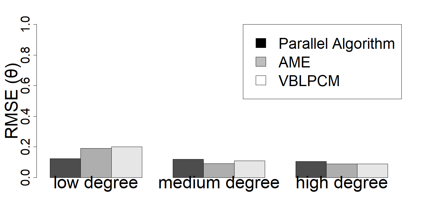
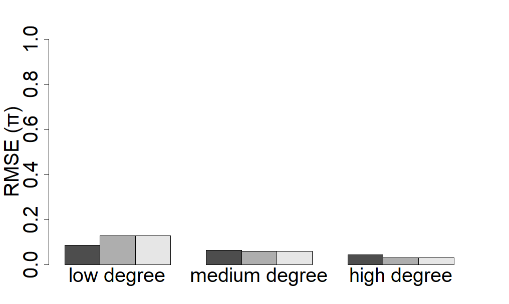
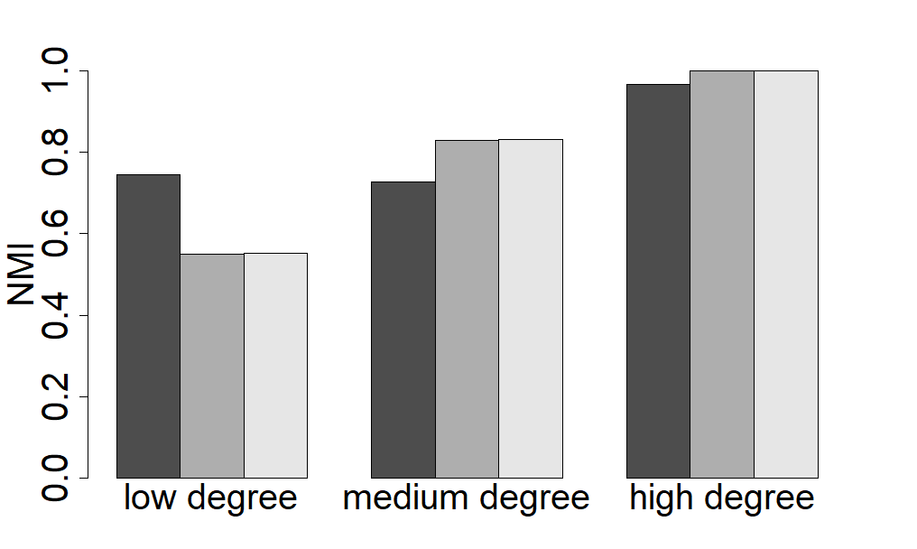
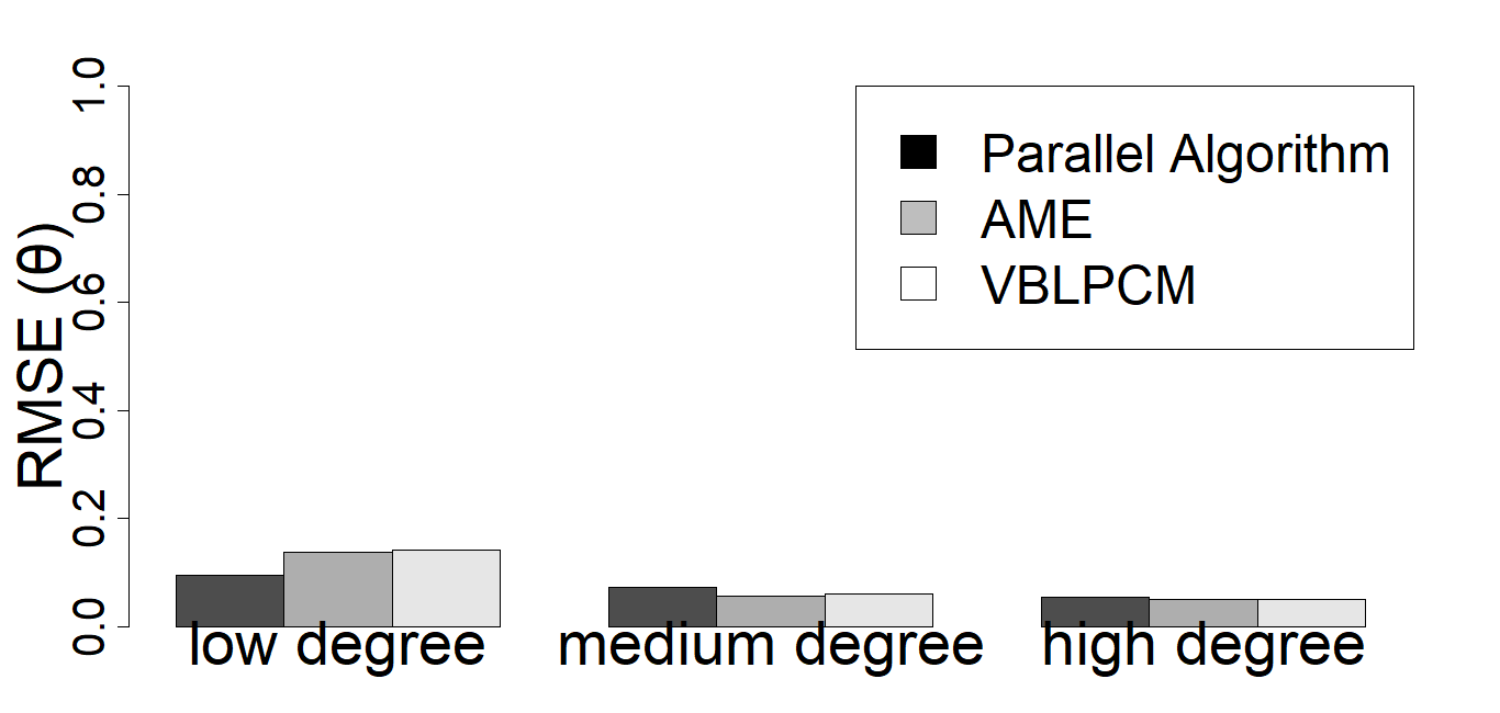
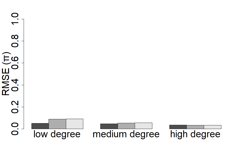
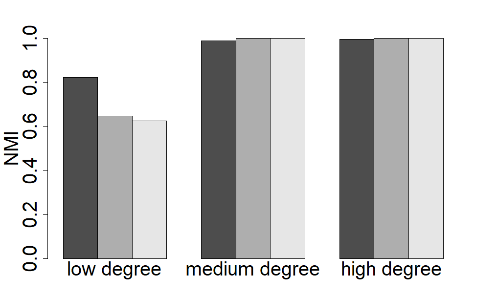
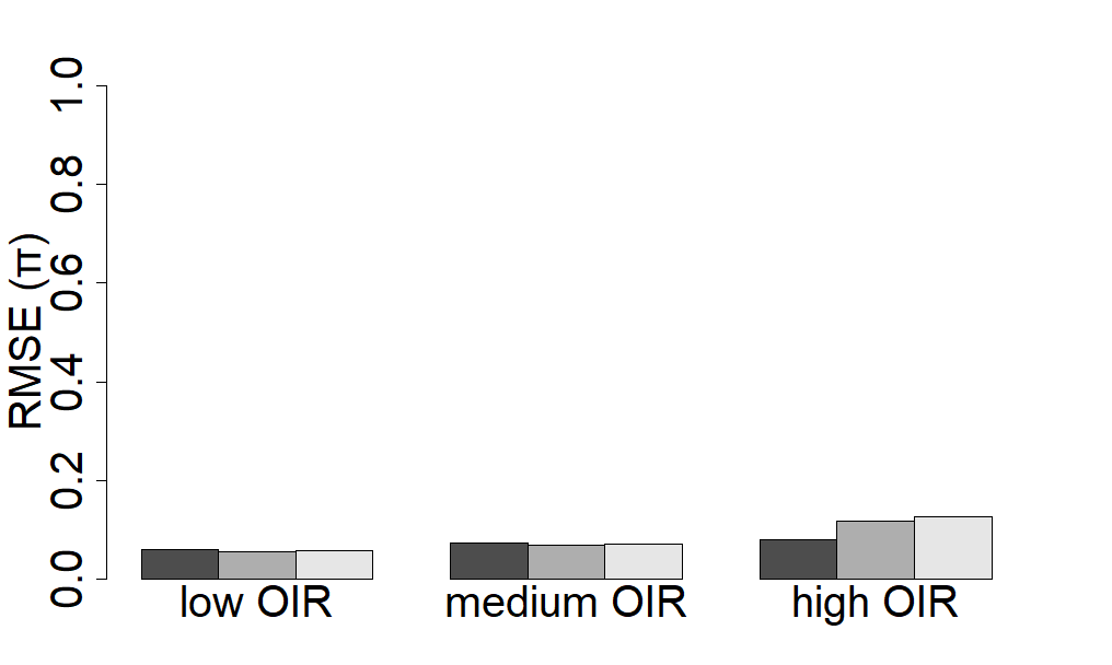
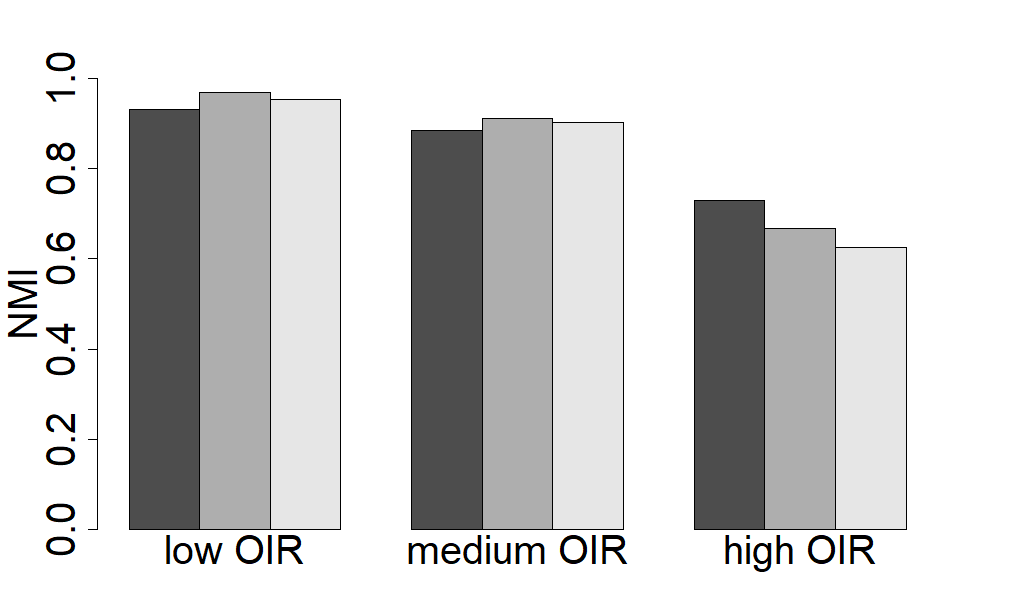
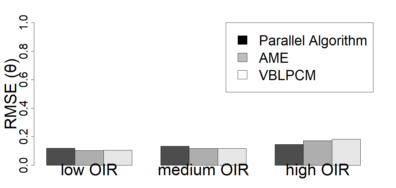
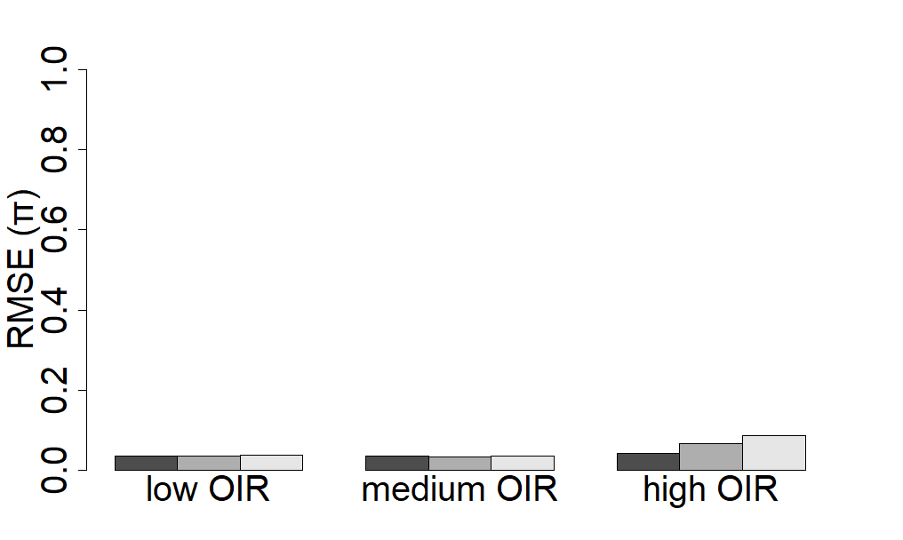
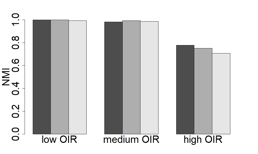
We also compare the proposed modeling approach and Algorithm 4 to two other models in the literature- (1) an additive and mixed effects model focusing on dyadic networks (AMEN) (Hoff (2005, 2015)) and (2) a latent position cluster model using Variational Bayes implementation (VBLPCM) (Salter-Townshend and Murphy (2013)). As before, we use two different settings- balanced and unbalanced community size and make the comparison in the bar diagrams given in Figures 1 and  2, respectively. Also in one case, we keep the average degree $\lambda$ fixed at 8 and vary OIR as $(0.04,0.08,0.2)$, while on another occasion we fix OIR at 0.04 and vary $\lambda$ as $(4,8,14)$. To compare the performance of our parallel communication algorithm to AMEN and VBLPCM with respect to community detection, we use bar diagrams of the NMI values under the settings described above. Based on the results depicted in Figures 1 and 2, we observe that both AMEN and VBLPCM tend to exhibit a slightly better performance in terms of NMI values and RMSE of parameter estimates when OIR is low (assortative network structure) or medium and $\lambda$ is medium or high. Our parallel algorithm tends to perform significantly better than both AMEN and VBLPCM when OIR is high and $\lambda$ is low. In fact, gains for AMEN and VBLPCM in terms of performance over Algorithm 4 in the mentioned settings are less compared to the gain of Algorithm 4 over its competitors in high OIR (disassortative network structure) and low $\lambda$ (sparse) settings. The simulation studies do convey the fact that for sparse networks and in cases where communities have high interactions (many real world networks have one or both of these features) amongst their member nodes, Algorithm 4 exhibits a superior performance compared to AMEN or VBLPCM for likelihood based inference in SBMs.

Table 2: Comparison of performance of three different methods for $\lambda=8$, $n=1000$, $K=3$ and balanced community size with varying OIR (bias of the estimates are given in parentheses)

OIR	Methods	est.err($\pi$)	est.err($\theta$)	est.err($\beta$)	NMI
0.04	MCEM on Full Data	0.0313	0.0893	0.0185	1.0000
	Parallel Communication	0.0340 (0.0020)	0.0987 (0.0049)	0.0232 (0.0016)	1.0000
	Parallel Non-communication	0.0483 (0.0039)	0.1194 (0.0078)	0.0433 (0.0035)	0.9000
0.08	MCEM on Full Data	0.0321	0.0916	0.0228	0.9876
	Parallel Communication	0.0349 (0.0024)	0.1042 (0.0060)	0.0320 (0.0020)	0.9830
	Parallel Non-communication	0.0568 (0.0043)	0.1377 (0.0104)	0.0549 (0.0039)	0.8939
0.2	MCEM on Full Data	0.0385	0.0988	0.0378	0.7916
	Parallel Communication	0.0406 (0.0029)	0.1061 (0.0079)	0.0476 (0.0036)	0.7796
	Parallel Non-communication	0.0617 (0.0358)	0.1459 (0.0671)	0.0701 (0.0091)	0.7534

Table 3: Comparison of performance of three different methods for $\lambda=8$, $n=1000$, $K=3$ and unbalanced community size with varying OIR (bias of the estimates are given in parentheses)

OIR	Methods	est.err($\pi$)	est.err($\theta$)	est.err($\beta$)	NMI
0.04	MCEM on Full Data	0.0511	0.0879	0.0412	0.9510
	Parallel Communication	0.0604 (0.0036)	0.0937 (0.0047)	0.0644 (0.0045)	0.9327
	Parallel Non-communication	0.0782 (0.0051)	0.1185 (0.0077)	0.0750 (0.0053)	0.8681
0.08	MCEM on Full Data	0.0589	0.0933	0.0612	0.9054
	Parallel Communication	0.0736 (0.0048)	0.1048 (0.0068)	0.0732 (0.0051)	0.8852
	Parallel Non-communication	0.0874 (0.0065)	0.1253 (0.0125)	0.0867 (0.0069)	0.8428
0.2	MCEM on Full Data	0.0657	0.1041	0.0804	0.8251
	Parallel Communication	0.0803 (0.0058)	0.1187 (0.0088)	0.0954 (0.0072)	0.7896
	Parallel Non-communication	0.1010 (0.0586)	0.1503 (0.0691)	0.1309 (0.0170)	0.7314

Table 4: Comparison of performance of three different methods for $OIR=0.04$, $n=1000$, $K=3$ and balanced community size with varying $\lambda$ (bias of the estimates are given in parentheses)

$\lambda$	Methods	est.err($\pi$)	est.err($\theta$)	est.err($\beta$)	NMI
4	MCEM on Full Data	0.0467	0.0885	0.0455	0.8532
	Parallel Communication	0.0508 (0.0037)	0.0948 (0.0070)	0.0516 (0.0049)	0.8240
	Parallel Non- communication	0.0664 (0.0385)	0.1343 (0.0698)	0.0724 (0.0145)	0.8084
8	MCEM on Full Data	0.0389	0.0703	0.0393	0.9976
	Parallel Communication	0.0451 (0.0028)	0.0721 (0.0053)	0.0487 (0.0034)	0.9889
	Parallel Non-communication	0.0604 (0.0054)	0.0925 (0.0148)	0.0613 (0.0061)	0.9670
14	MCEM on Full Data	0.0302	0.0508	0.0297	1.0000
	Parallel Communication	0.0340 (0.0020)	0.0540 (0.0035)	0.0354 (0.0025)	0.9968
	Parallel Non-communication	0.0515 (0.0031)	0.0805 (0.0056)	0.0575 (0.0046)	0.9856

Table 5: Comparison of performance of three different methods for $OIR=0.04$, $n=1000$, $K=3$ and unbalanced community size with varying $\lambda$ (bias of the estimates are given in parentheses)

$\lambda$	Methods	est.err($\pi$)	est.err($\theta$)	est.err($\beta$)	NMI
4	MCEM on Full Data	0.0778	0.1189	0.0651	0.7832
	Parallel Communication	0.0853 (0.0061)	0.1244 (0.0092)	0.0706 (0.0053)	0.7447
	Parallel Non-communication	0.1052 (0.0610)	0.1605 (0.0738)	0.1082 (0.0141)	0.7192
8	MCEM on Full Data	0.0554	0.1087	0.0543	0.8982
	Parallel Communication	0.0628 (0.0041)	0.1186 (0.0071)	0.0612 (0.0043)	0.8681
	Parallel Non-communication	0.0815 (0.0059)	0.1419 (0.0114)	0.0811 (0.0081)	0.8337
14	MCEM on Full Data	0.0368	0.0974	0.0410	0.9889
	Parallel Communication	0.0433 (0.0026)	0.1047 (0.0052)	0.0478 (0.0033)	0.9668
	Parallel Non-communication	0.0575 (0.0040)	0.1286 (0.0077)	0.0695 (0.0049)	0.9334

Figure 1: Comparison of Algorithm 4 to the additive and mixed effect linear models in networks (AMEN) and a variational Bayes implementation of latent position cluster model (VBLPCM) for parameter estimation in Stochastic Blockmodels for low, medium and high degree networks, respectively. Top row corresponds to the unbalanced, while bottom row to the balanced community size case, respectively.

Figure 2: Comparison of Algorithm 4 to the additive and mixed effect linear models in networks (AMEN) and a variational Bayes implementation of latent position cluster model (VBLPCM) for parameter estimation in Stochastic Blockmodels for low, medium and high OIR networks, respectively. Top row corresponds to the unbalanced, while bottom row to the balanced community size case, respectively.

5 Application to Collegiate Facebook Data

We use the proposed model to analyze a publicly available social network data set. The data come from https://archive.org/details/oxford-2005-facebook-matrix that contains the social structure of Facebook friendship networks at one hundred American colleges and universities at a single point in time. This data set was analyzed by Traud et al. (2012) . The focus of their study was to illustrate how the relative importance of different characteristics of individuals vary across different institutions. They examine the influence of the common attributes at the dyad level in terms of assortativity coefficients and regression models. We on the other hand pick a data set corresponding to a particular university and show the performance of our algorithm and compare the clusters obtained from it with the ones obtained in case of fitting an SBM without covariates.
We examine the Rice University data set from the list of one hundred American colleges and universities and use our K-class SBM with and without covariates to identify group/community structures in the data set. We examine the role of the user attributes- dorm/house number, gender and class year along with the latent structure.
Dorm/house number is a multi-category variable taking values as 202, 203, 204 etc., gender is a binary ($\left\{0,1\right\}$) variable and class year is a integer valued variable (e.g. “2004”, “2005”, “2006” etc.). We evaluate the performance of Algorithm 4 fitted to SBM with covariate viz. model (1).
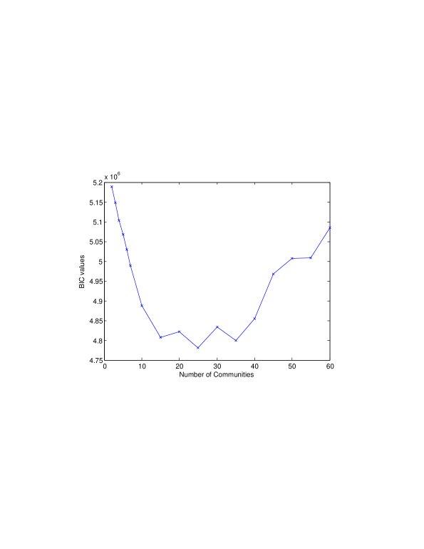
There are some missing values in the data set although it is only around 5%. Since the network size is 4087 which is large enough, we discard the missing value cases. We also consider the covariate values only between year 2004 to 2010. Further, we drop those nodes with degree less than or equal to 1. After this initial cleaning up, the adjacency matrix is of order $3160\times 3160$. We choose number of communities $K=20$. The choice of the number of communities is made by employing Bayesian Information Criterion (BIC) where the observed data likelihood is computed by path sampling (Gelman and Meng (1998)). The corresponding plot is given in Figure 3 where the possible number of communities are plotted along the horizontal axis and the BIC values along the vertical one.

Figure 3: Choice of the number of clusters (communities) in the Rice University Dataset. Plot of BIC values over possible number of clusters in the Dataset.

Recall the K-class SBM with covariates

$$\log\frac{P_{ij}}{1-P_{ij}}=\theta_{z_{i}z_{j}}+\beta^{T}X(i,j)\mbox{ $i=1,\ldots,n;j=i+1,\ldots,n$ }$$ (10)

where $P$ is the matrix describing the probability of the edges between any two individuals in the network and the probability of a link between $i$ and $j$ is assumed to be composed of the “latent” part given by $\theta_{z_{i}z_{j}}$ and the “covariate” part given by $\beta^{T}X(i,j)$ where $\beta$ is a parameter of size $3\times 1$ and $X(i,j)$ a vector of covariates of the same order indicating shared group membership. The vector $\beta$ is implemented here with sum to zero identifiability constraints.
We apply Algorithm 4 to fit model (10) to the Rice university facebook network with three covariates dorm/house number, gender and class year.
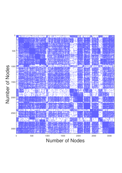
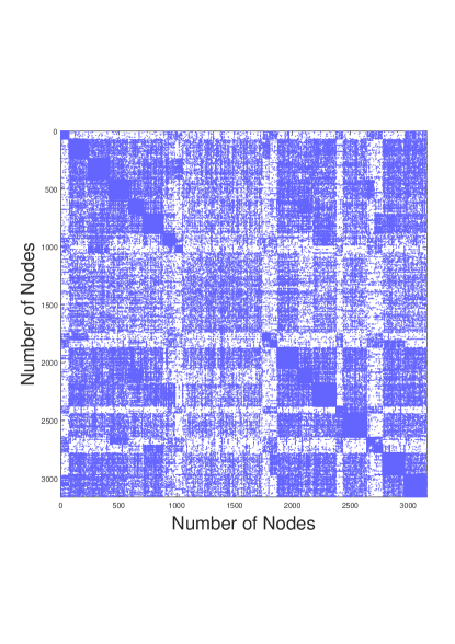
We plot the communities found by fitting a SBM without covariates ($\beta=0$ in model (1)) and a blockmodel with covariates to the given data. Let $\mathcal{C}$ and $\mathcal{C}$ be the two sets of clustering obtained by fitting with and without covariate blockmodel respectively. We define a measure called Minimal Matching Distance (MMD)(Von Luxburg et al. (2010)) to find a best greedy 1-1 matching between the two sets of cluster. Suppose $\Pi=\left\{\pi\right\}$ denote the set of all permutations of $k$ labels. Then MMD is defined as

$$\text{MMD}=\frac{1}{n}\min_{\pi\in\Pi}\displaystyle\sum_{i=1}^{n}1_{\mathcal{C}(i)\neq\mathcal{C}^{\prime}(i)}$$

where $\mathcal{C}(i)$ ($\mathcal{C}^{\prime}(i)$ respectively) denote the clustering label of $i$ in $\mathcal{C}$ ($\mathcal{C}^{\prime}(i)$ respectively). Finding the best permutation then reduces to a problem of maximum bipartite matching and we align the two sets of clustering (with and without covariate) by finding the maximum overlap between the two sets of cluster. The two sets of clustering solutions (with and without covariates respectively) are plotted in Fig. 4. The estimate of the parameter beta linked with the covariate effects is given by

$$\hat{\beta}=[0.7956,-0.1738,-0.6218]^{\prime}$$

We compare this finding with the ones observed in Traud et al. (2012). They studied the “Facebook” friendships networks of one hundred American institutions at a given point of time. In particular, they calculate the assortativity coefficients and the regression coefficients based on the observed ties to understand homophily at the local level. Further, exploring the community structure reveals the corresponding macroscopic structure. For the Rice University data set, their findings support that residence/dorm number plays a key role in the organization of the friendship network. In fact, residence/dorm number provides the highest assortativity values for the Rice University network. We obtain a similar result, by observing that the effect of the first component of $\hat{\beta}$ is quite high. Further, their study reveals that class year also plays a strong role in influencing the community structure. This is again supported by our finding as the magnitude of the third component in $\hat{\beta}$ is sufficiently large. Finally, as seen in the analysis in Traud et al. (2012), gender plays a less significant role in the organization of the community structure; a similar conclusion is obtained by examining the magnitude of the second component of $\hat{\beta}$.

Figure 4: Community detection plots for parallel MCEM with and without covariate respectively. The two sets of clustering are very similar although the one with covariate (left) appears to be less noisy than the without covariate one (right).

Further, we employ the Normalized Mutual Information (NMI) to compare the two sets of clusters. The NMI between the two sets of clustering (with and without covariate) is 0.8071 which indicates that the two sets of clustering are quite close i.e. the effects of the covariates in clustering the individuals into groups are not strong.

6 Conclusion

Large heterogenous network data are ubiquitous in many application domains. The SBM framework is useful in analyzing networks with a community/group structure. Often, the interest lies in extracting the underlying community structure (inferring about the latent membership vector $z$) in the network, whereas in other situations (where the observed network can be thought of a sample from a large population) the interest lies in the estimation of the model parameters ($(\theta,\beta,\pi)$). There are certainly fast methods (e.g. the pseudo-likelihood based method in (Amini et al., 2013)) available for community detection in large networks, but these approximations are readily not applicable to settings when there is also covariate information available for the nodes. Further, comparison with some of the existing latent space models with covariates reveal that in certain settings (for sparse networks and in cases where communities have high interactions) our proposed algorithm performs much better than the existing ones. To obtain maximum likelihood estimates in a large SBM with covariates is computationally challenging. Traditional approaches like MCEM becomes computationally infeasible and hence there is a need for fast computational algorithms. Our proposed algorithm provides a solution in this direction.

The proposed parallel implementation of case-control MCEM across different cores with communication offers the following advantages: (1) fast computation of the ML estimates of the model parameters by reducing the EM update cost to $O(Km_{0}n_{0}M_{r})$ -$Km_{0}$ being the case-control sample size and $n_{0}$ the number of subsamples, from $O(n^{2}M_{r})$; (2) the parallel version with communication also exhibits further benefits over its non-communication counterpart, since it provides a bias reduction of the final estimates. It is evident from the results in Section 4 that the communications based variant performs much better than the non-communication one when compared to the MCEM on the full data.

7 Supplementary Materials

We provide the Matlab codes for the simulations and the real data analysis in the supplementary materials. The Rice University dataset is also provided there. We also provide additional two figures- (a) degree distribution of the Rice University network and (b) a plot of the estimated class probabilities for the covariate model inside the supplementary material. All the matrials are zipped into a file named $\verb supp_materials.zip$. This file include a detailed readme file that describes the contents and instructs the reader on their use. The readme file also contain diagrammatic representations of the two parallel algorithms. All the supplementary files are contained in a single archive and can be obtained via a single download.

References

- Agarwal and Duchi (2011) Agarwal, A. and J. C. Duchi (2011). Distributed delayed stochastic optimization. In Advances in Neural Information Processing Systems, pp. 873–881.
- Airoldi et al. (2008) Airoldi, E. M., D. M. Blei, S. E. Fienberg, and E. P. Xing (2008). Mixed membership stochastic blockmodels. Journal of Machine Learning Research 9, 1981–2014.
- Amini et al. (2013) Amini, A. A., A. Chen, P. J. Bickel, and E. Levina (2013, 08). Pseudo-likelihood methods for community detection in large sparse networks. Ann. Statist. 41(4), 2097–2122.
- Breslow et al. (1982) Breslow, N., N. Day, and J. J. Schlesselman (1982). Statistical methods in cancer research. volume 1-the analysis of case-control studies. Journal of Occupational and Environmental Medicine 24(4), 255–257.
- Breslow (1996) Breslow, N. E. (1996). Statistics in epidemiology: the case-control study. Journal of the American Statistical Association 91(433), 14–28.
- Choi et al. (2012) Choi, D. S., P. J. Wolfe, and E. M. Airoldi (2012). Stochastic blockmodels with a growing number of classes. Biometrika, asr053.
- Decelle et al. (2011) Decelle, A., F. Krzakala, C. Moore, and L. Zdeborová (2011). Asymptotic analysis of the stochastic block model for modular networks and its algorithmic applications. Physical Review E 84(6), 066106.
- Dekel et al. (2012) Dekel, O., R. Gilad-Bachrach, O. Shamir, and L. Xiao (2012). Optimal distributed online prediction using mini-batches. The Journal of Machine Learning Research 13(1), 165–202.
- Duchi et al. (2012) Duchi, J. C., A. Agarwal, and M. J. Wainwright (2012). Dual averaging for distributed optimization: convergence analysis and network scaling. Automatic Control, IEEE Transactions on 57(3), 592–606.
- Fithian and Hastie (2014) Fithian, W. and T. Hastie (2014). Local case-control sampling: Efficient subsampling in imbalanced data sets. Annals of statistics 42(5), 1693.
- Fortunato (2010) Fortunato, S. (2010). Community detection in graphs. Physics reports 486(3), 75–174.
- Gelman and Meng (1998) Gelman, A. and X.-L. Meng (1998). Simulating normalizing constants: From importance sampling to bridge sampling to path sampling. Statistical science, 163–185.
- Girvan and Newman (2002) Girvan, M. and M. E. Newman (2002). Community structure in social and biological networks. Proceedings of the National Academy of Sciences 99(12), 7821–7826.
- Handcock et al. (2007) Handcock, M. S., A. E. Raftery, and J. M. Tantrum (2007). Model-based clustering for social networks. Journal of the Royal Statistical Society: Series A (Statistics in Society) 170(2), 301–354.
- Hoff (2005) Hoff, P. D. (2005). Bilinear mixed-effects models for dyadic data. Journal of the american Statistical association 100(469), 286–295.
- Hoff (2015) Hoff, P. D. (2015). Dyadic data analysis with amen. arXiv preprint arXiv:1506.08237.
- Hoff et al. (2002) Hoff, P. D., A. E. Raftery, and M. S. Handcock (2002). Latent space approaches to social network analysis. Journal of the american Statistical association 97(460), 1090–1098.
- Holland et al. (1983) Holland, P. W., K. B. Laskey, and S. Leinhardt (1983). Stochastic blockmodels: First steps. Social networks 5(2), 109–137.
- Johansson et al. (2009) Johansson, B., M. Rabi, and M. Johansson (2009). A randomized incremental subgradient method for distributed optimization in networked systems. SIAM Journal on Optimization 20(3), 1157–1170.
- Latouche et al. (2018) Latouche, P., S. Robin, and S. Ouadah (2018). Goodness of fit of logistic regression models for random graphs. Journal of Computational and Graphical Statistics 0(0), 1–12.
- Ma and Ma (2017) Ma, Z. and Z. Ma (2017). Exploration of large networks via fast and universal latent space model fitting. arXiv preprint arXiv:1705.02372.
- Mariadassou et al. (2010) Mariadassou, M., S. Robin, and C. Vacher (2010). Uncovering latent structure in valued graphs: a variational approach. The Annals of Applied Statistics, 715–742.
- McDonald et al. (2010) McDonald, R., K. Hall, and G. Mann (2010). Distributed training strategies for the structured perceptron. In Human Language Technologies: The 2010 Annual Conference of the North American Chapter of the Association for Computational Linguistics, pp. 456–464. Association for Computational Linguistics.
- Mcdonald et al. (2009) Mcdonald, R., M. Mohri, N. Silberman, D. Walker, and G. S. Mann (2009). Efficient large-scale distributed training of conditional maximum entropy models. In Advances in Neural Information Processing Systems, pp. 1231–1239.
- Nedic and Ozdaglar (2009) Nedic, A. and A. Ozdaglar (2009). Distributed subgradient methods for multi-agent optimization. Automatic Control, IEEE Transactions on 54(1), 48–61.
- Nowicki and Snijders (2001) Nowicki, K. and T. A. B. Snijders (2001). Estimation and prediction for stochastic blockstructures. Journal of the American Statistical Association 96(455), 1077–1087.
- Raftery et al. (2012) Raftery, A. E., X. Niu, P. D. Hoff, and K. Y. Yeung (2012). Fast inference for the latent space network model using a case-control approximate likelihood. Journal of Computational and Graphical Statistics 21(4), 901–919.
- Ram et al. (2010) Ram, S. S., A. Nedić, and V. V. Veeravalli (2010). Distributed stochastic subgradient projection algorithms for convex optimization. Journal of optimization theory and applications 147(3), 516–545.
- Recht et al. (2011) Recht, B., C. Re, S. Wright, and F. Niu (2011). Hogwild: A lock-free approach to parallelizing stochastic gradient descent. In Advances in Neural Information Processing Systems, pp. 693–701.
- Robert and Casella (2013) Robert, C. and G. Casella (2013). Monte Carlo Statistical Methods. Springer Science & Business Media.
- Rohe et al. (2011) Rohe, K., S. Chatterjee, and B. Yu (2011). Spectral clustering and the high-dimensional stochastic blockmodel. The Annals of Statistics, 1878–1915.
- Salter-Townshend and Murphy (2013) Salter-Townshend, M. and T. B. Murphy (2013). Variational bayesian inference for the latent position cluster model for network data. Computational Statistics & Data Analysis 57(1), 661–671.
- Snijders and Nowicki (1997) Snijders, T. A. and K. Nowicki (1997). Estimation and prediction for stochastic blockmodels for graphs with latent block structure. Journal of classification 14(1), 75–100.
- Tallberg (2004) Tallberg, C. (2004). A bayesian approach to modeling stochastic blockstructures with covariates. Journal of Mathematical Sociology 29(1), 1–23.
- Traud et al. (2012) Traud, A. L., P. J. Mucha, and M. A. Porter (2012). Social structure of facebook networks. Physica A: Statistical Mechanics and its Applications 391(16), 4165–4180.
- Von Luxburg et al. (2010) Von Luxburg, U. et al. (2010). Clustering stability: an overview. Foundations and Trends® in Machine Learning 2(3), 235–274.
- Wei and Tanner (1990) Wei, G. C. and M. A. Tanner (1990). A monte carlo implementation of the em algorithm and the poor man’s data augmentation algorithms. Journal of the American statistical Association 85(411), 699–704.
- White and Smyth (2005) White, S. and P. Smyth (2005). A spectral clustering approach to finding communities in graph. In SDM, Volume 5, pp. 76–84. SIAM.
- Zhang et al. (2013) Zhang, Y., J. C. Duchi, and M. J. Wainwright (2013). Communication-efficient algorithms for statistical optimization. Journal of Machine Learning Research 14, 3321–3363.
- Zinkevich et al. (2010) Zinkevich, M., M. Weimer, L. Li, and A. J. Smola (2010). Parallelized stochastic gradient descent. In Advances in Neural Information Processing Systems, pp. 2595–2603.