Convergence of the Critical Planar Ising Interfaces to Hypergeometric SLE
Abstract
We consider the planar Ising model in rectangle with alternating boundary condition: along and , along , and along . We prove that the interface of critical Ising model with these boundary conditions converges to the so-called hypergeometric SLE3. The method developed in this paper does not require constructing new holomorphic observable and the input is the convergence of the interface with Dobrushin boundary condition. This method could be applied to other lattice models, for instance Loop-Erased Random Walk and level lines of discrete Gaussian Free Field.
Keywords: Critical Planar Ising, Hypergeometric SLE.
1 Introduction
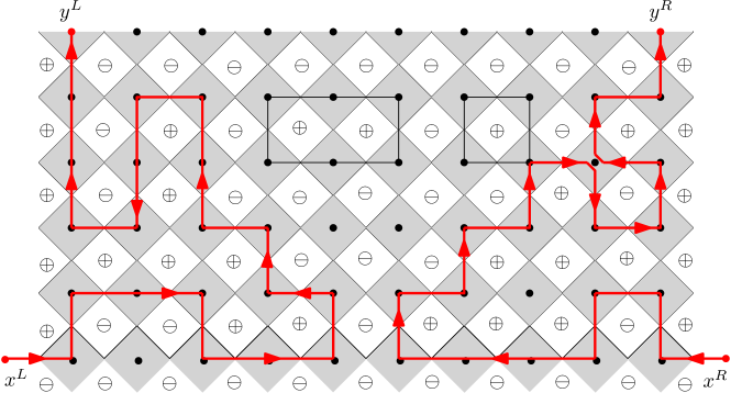
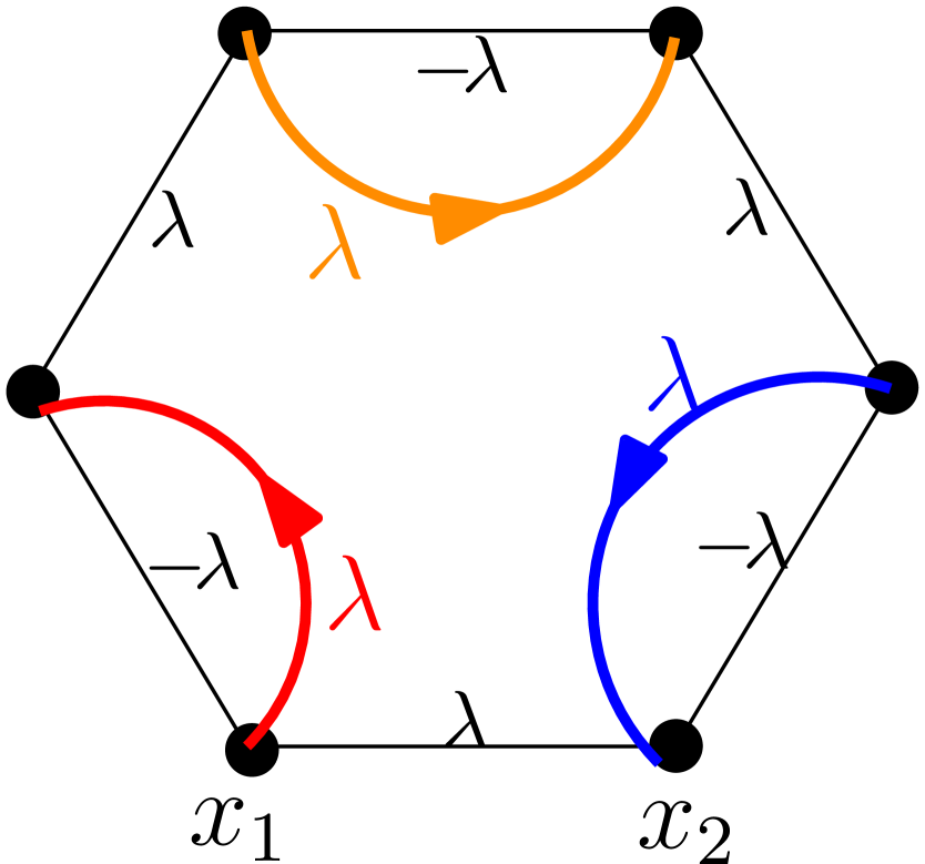
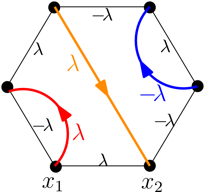
The Lenz-Ising model is introduced to model the ferromagnetism in statistical mechanics. Due to celebrated work of Chelkak and Smirnov [CS12], it is proved that at the critical temperature, the interface of Ising model is conformally invariant. In particular, the interface of critical Ising model with Dobrushin boundary condition converges to [CDCH+14], and the interface of critical Ising model with free boundary condition converges to [HK13, Izy15], and the interface for multiply-connected domains [Izy13]. In these cases, the proofs are based on constructing holomorphic observables. In this paper, we study the scaling limit of the critical Ising model with alternating boundary conditions: we consider critical Ising model in a rectangle with along and , along , and along . With these boundary conditions, on the event that there is a vertical crossing of , we see that there are two interfaces in the model where is an interface from to and is an interface from to . In this paper, we study the law of the pair . The scaling limit of is the so-called hypergeometric SLE, denoted by .
There are two features on the method developed in this paper. First, constructing holomorphic observable is the usual way to prove the convergence of interfaces in the critical lattice model; however, with our method, there is no need to construct new observable. The only input we need is the convergence of the interface with Dobrushin boundary condition. Second, there are many works on multiple SLEs trying to study the scaling limit of interfaces in critical lattice model with alternating boundary conditions, see [Dub07, BBK05, KP16], and their works study the local growth of these interfaces. Whereas, our result is “global": we prove that the scaling limit of is as a continuous curve from to . Moreover, the method developed in this paper also works for other lattice models as long as we have the convergence with Doburshin boundary conditions, for instance Loop-Erased Random Walk and level lines of discrete Gaussian Free Field.
In this paper, we first study the properties of in Theorem 1.1. Then we study the possible scaling limit of the pair of the interfaces . We realize that there exists only one possible candidate for the limit of the pair , see Theorem 1.2. By identifying the only possible candidate, we prove the convergence of the pair of the interfaces in the critical Ising model with alternating boundary condition in Theorem 1.3. In particular, this gives the convergence of to .
Theorem 1.1.
Fix , and . Let be the in from to with marked points . The process is almost surely generated by a continuous transient curve. Moreover, the process enjoys reversibility for : the time reversal of is the in from to with marked points .
Theorem 1.2.
Fix a topological rectangle . Let be the collection of pairs of continuous curves in such that (resp. ) is a continuous curve from to (resp. from to ) that does not intersect (resp. does not intersect ) and that is to the left of . Fix and .
-
•
(Existence and Uniqueness) There exists a unique probability measure on with the following property: the conditional law of given is with force point in the connected component of with on the boundary, and the conditional law of given is with force point in the connected component of with on the boundary.
-
•
(Identification) Under this probability measure and fix and , the marginal law of is with marked points .
Theorem 1.3.
Let discrete domains on the square lattice approximate some topological rectangle as . Consider the critical Ising model in with the alternating boundary condition: on and , on , and on . Conditioned on the event that there exists a vertical crossing of , then there exists a pair of interfaces where (resp. ) is the interface connecting to (resp. connecting to ). The law of the pair converges weakly to the pair of curves in Theorem 1.2 as where and are related in the following way: for ,
In particular, when and , the law of converges weakly to as ; when and , the law of converges weakly to as .
A similar conclusion as in Theorem 1.2 also holds for multiple curves; however, we can only identify the marginal law for the case , see Remark 4.4, and it is difficult to identify the marginal law of the curves for general . Instead, we could derive the marginal law for the degenerate case: when all the starting points of curves coincide and all the ending points of curves coincide, the marginal law of the curves becomes process.
Proposition 1.4.
Fix a Dobrushin domain and an integer . Let be the collection of non-intersecting curves where is a continuous curve in from to for and that is to the right of and is to the left of with the convention that and . Fix .
-
•
(Existence and Uniqueness) There exists a unique probability measure on with the following property: for each , the conditional law of given and is in the region between and .
-
•
(Identification) Under this probability measure, the marginal law of is for where .
In Theorem 1.2 and Proposition 1.4, we focus on . Readers may wonder whether we have similar conclusion for . In fact, we believe the conclusion in Theorem 1.2 also holds for . However, both of the two parts are unknown to our knowledge. Whereas, we can still show a weaker version of Theorem 1.2 for the degenerate case when , see Lemma 4.5. By applying this result to FK-Ising model, we have the following conclusion.
Proposition 1.5.
Let discrete domains on the square lattice approximate some Dobrushin domain such that and as . Consider the critical FK-Ising model in with alternating boundary condition: free on and , and wired on and . Conditioned on the event that there are two disjoint vertical dual-crossings, then there exists a pair of interfaces where (resp. ) is the interface connecting to (resp. connecting to ). The law of converges weakly to the unique pair of curves in with the following property: Given , the conditional law of is an conditioned not to hit except at the end points; given , the conditional law of is an conditioned not to hit except at the end points. In particular, the law of converges weakly to with as .
To end the introduction, we summarize the relation between and process:
-
•
When , process is the same as .
-
•
When , process is the same as with force points .
-
•
When , process degenerates to with force point .
Outline and relation to previous work. We will introduce hypergeometric SLE in Section 3. There were various papers working on variants of hypergeometric SLE with different motivations, see [Zha08, Qia16]. The definitions may be different from ours. There are some technicalities that arise when introducing hypergeometric SLE that do not have been fully addressed previously. We include a self-contained introduction to with our motivation in Section 3, treat the technical difficulties and show Theorem 1.1. We will prove Theorem 1.2 and Proposition 1.4 in Section 4. The uniqueness part in Theorem 1.2 was proved in [MS16b, Theorem 4.1] and the existence part when was proved in [Law09, KL07]. We will introduce Ising model in Section 5 and prove Theomem 1.3. We will introduce FK-Ising model in Section 6 and prove Proposition 1.5. In [Izy13], the author proved “local" convergence of Ising interfaces to by constructing holomorphic observables. We will show Theorem 1.3 by Theorem 1.2 (without constructing any new observable). Our approach is “global", the method only requires the input of convergence with Dobrushin boundary condition and it also works for other lattice models.
2 Preliminaries
2.1 Space of curves
A planar curve is a continuous mapping from to modulo reparameterization. Let be the set of planar curves. The metric on is defined by
where the inf is over increasing homeomorphisms . The metric space is complete and separable. A simple curve is a continuous injective mapping from to modulo reparameterization. Let be the subspace of simple curves and denote by its closure. The curves in may have multiple points but they do not have self-crossings.
We call a Dobrushin domain if is a non-empty simply connected proper subset of and are two distinct boundary points. Denote by the arc of from to counterclockwise. We say that a sequence of Dobrushin domains converges to a Dobrushin domain in the Carathéodory sense if uniformly on any compact subset of where (resp. ) is the unique conformal map from to (resp. ) satisfying and (resp. ).
Given a Dobrushin domain , let be the space of simple curves such that
Denote by the closure of .
We call a quad (or topological rectangle) if a non-empty simply connected proper subset of and are four distinct boundary points in counterclockwise order. Given a quad , we denote by the extremal distance between and in . We say a sequence of quads converges to a quad in the Carathéodory sense if uniformly on any compact subset of and and where (resp. ) is the unique conformal map from to (resp. ) satisfying and (resp. ).
Given a quad , let be the collection of pairs of simple curves such that and and that . The definition of is a little bit complicate. Given a quad and , let be the set of pairs of curves such that
-
•
and ;
-
•
where the connected component of with on the boundary, and is contained in the closure of ;
-
•
where the connected component of with on the boundary, and is contained in the closure of .
Define the metric on by
One can check is a metric and the space with is complete and separable. Finally, set
Note that is no longer complete.
Suppose is a metric space and is the Borel -field. Let be the space of probability measures on . The Prohorov metric on is defined by
When is complete and separable, the space is complete and separable ([Bil99, Theorem 6.8]); moreover, a sequence in converges weakly to if and only if .
Let be a family of probability measures on . We call relatively compact if every sequence of elements in contains a weakly convergent subsequence. We call tight if, for every , there exists a compact set such that for all . By Prohorov’s Theorem ([Bil99, Theorem 5.2]), when is complete and separable, relative compactness is equivalent to tightness.
2.2 Loewner chain
We call a compact subset of an -hull if is simply connected. Riemann’s Mapping Theorem asserts that there exists a unique conformal map from onto such that . We call such the conformal map from onto normalized at and we call the half-plane capacity of .
Loewner chain is a collection of -hulls associated with the family of conformal maps obtained by solving the Loewner equation: for each ,
where is a one-dimensional continuous function which we call the driving function. Let be the swallowing time of defined as . Let . Then is the unique conformal map from onto normalized at . Since the half-plane capacity for is for all , we say that the process is parameterized by the half-plane capacity. We say that can be generated by the continuous curve if for any , the unbounded connected component of coincides with .
Here we discuss about the evolution of a point under . We assume . There are two possibilities: if is not swallowed by , then we define ; if is swallowed by , then we define to be the image of the rightmost of point of under . Suppose that is generated by a continuous path and that the Lebesgue measure of is zero. Then the process is uniquely characterized by the following equation:
In this paper, we may write for the process .
The convention of driving function can be defined for any simply connected domain via conformal transformation. Fix a Dobrushin domain and let be some fixed conformal map from onto such that and . Suppose . Then is a continuous curve in . Thus, if we parameterize by its half-plane capacity, then it has a continuous driving process. We use the term the driving process of in to indicate the driving process in half-plane capacity in after the transformation .
2.3 Convergence of curves
In this section, we first recall the main result of [KS12] and then show a similar result for pairs of curves. Suppose is a quad. We say that a curve crosses if there exists a subinterval such that and intersects both and . Fix a Dobrushin domain , for any curve in and any time , define to be the connected component of with on the boundary. Consider a quad in such that and are contained in . We say that is avoidable if it does not disconnect from in .
Definition 2.1.
A family of probability measures on curves in is said to satisfy Condition C2 if, for any , there exists a constant such that for any , any stopping time , and any avoidable quad in such that , we have
Theorem 2.2.
[KS12, Corollary 1.7, Proposition 2.6]. Fix a Dobrushin domain . Suppose that is a sequence of curves in satisfying Condition C2. Denote by the driving process of . Then
-
•
the family is tight in the metrisable space of continuous functions on with the topology of uniform convergence on compact subsets of ;
-
•
the family is tight in the space of curves ;
-
•
the family , when each curve is parameterized by the half-plane capacity, is tight in the metrisable space of continuous functions on with the topology of uniform convergence on compact subsets of .
Moreover, if the sequence converges in any of the topologies above it also converges in the two other topologies and the limits agree in the sense that the limiting random curve is driven by the limiting driving function.
Next, we will explain a similar result for pairs of curves. Fix a quad .
Definition 2.3.
A family of probability measures on pairs of curves in is said to satisfy Condition C2 if, for any , there exists a constant such that for any , the following holds. Given any -stopping time and any -stopping time , and any avoidable quad for in such that , and any avoidable quad for in such that , we have
Theorem 2.4.
Suppose that is a sequence of pairs of curves in and denote their laws by . Let be the connected component of with on the boundary and be the connected component of with on the boundary. Define, for each ,
Assume that the family satisfies Condition C2 and that the sequence of random variables is tight in the following sense: for any , there exists such that
Then the sequence is relatively compact in .
Proof.
By Theorem 2.2, we know that there is subsequence such that (resp. ) converges weakly in all three topologies in Theorem 2.2. By Skorohod Represnetation Theorem, we could couple all in a common space so that and almost surely. For , define
From the assumption, we know that, for any , there exists such that . Therefore, with probability at least , the sequence converges to in . This is true for any , thus we have converges to in almost surely. ∎
2.4 SLE and SLE
Schramm Loewner Evolution is the random Loewner chain driven by where is a standard one-dimensional Brownian motion. In [RS05], the authors prove that is almost surely generated by a continuous transient curve, i.e. there almost surely exists a continuous curve such that for each , is the unbounded connected component of and that . There are phase transitions at and : are simple curves when ; they have self-touching when ; and they are space-filling when .
It is clear that is scaling invariant, thus we can define in any simply connected domain from one boundary point to another boundary point by the conformal image: let be a conformal map from onto that sends to and to , then define to be in from to . For , the curves enjoys reversibility: let be an in from to , then the time-reversal of has the same law as in from to . The reversibility for was proved in [Zha08], and it was proved for in [MS16c].
Hypergeometric functions are defined for , and for by
where is the Pochhammer symbol defined by for and for . When , denote by the Gamma function, we have (see [AS92, Equation (15.1.20)]),
The hypergeometric function is a solution of Euler’s hypergeometric differential equation:
In this paper, we focus on , , and
| (2.1) |
When , we have . In particular, is smooth for and is continuous for .
Lemma 2.5.
Fix , suppose is an in from 0 to and is the corresponding family of conformal maps. Fix and let be the swallowing time of . Define, for ,
Let be defined through (2.1). Then the following process is a local martingale:
Proof.
By Itô’s formula, one can check
Therefore, the process is a local martingale if is twice-differentiable and satisfies
One can check that satisfies this ODE and hence is a local martingale. Moreover, we have
We will show that is actually a uniform integrable martingale when in Proposition 3.4. ∎
processes are variants of where one keeps track of multiple points on the boundary. Suppose where and where and where for and . An process with force points is the Loewner evolution driven by which is the solution to the system of integrated SDEs:
| (2.2) | ||||
where is one-dimensional Brownian motion. Define the continuation threshold to be the infimum of the time for which
The process is well-defined up to the continuation threshold, and it is generated by continuous curve up to and including the continuation threshold, see [MS16a].
In this paper, we only use with two force points: with force points or with force points . To simply notations, we only discuss properties of these two kinds of processes. The behavior of varies according to different , see [Dub09, Lemma 15]. We list some of them that will be helpful later.
-
•
If , the curve never hits the interval . If , the curve never hits the interval .
-
•
If and , the curve hits the interval at finite time.
-
•
If and , the curve accumulates at the point at finite time.
By Girsanov’s Theorem, the law of process can be obtained by weighting the law of ordinary , see [SW05, Theorem 6]:
Lemma 2.6.
Fix and . Let be an in from 0 to and be the corresponding family of conformal maps. Define
Then is a local martingale for and the law of weighted by is equal to the law of with force points up to the swallowing time of .
Lemma 2.7.
Fix . For , let be the law of conditioned not to hit the interval . Then converges weakly to as .
Proof.
Let be an and denote by its law. By Lemma 2.6, we know that the process:
is a local martingale for and the law of weighted by becomes up to the first time that swallows . Since does not hit the interval , we know that is in fact a uniformly integrable martingale and the law of weighted by is for all time. For , define . By Optional Stopping Theorem, we have , thus the event has probability . Therefore, weighting the law of by is equivalent to conditioning on up to . This is true for all , thus weighting the law of by is equivalent to conditioning not to hit the interval . ∎
2.5 Gaussian Free Field
Suppose that is a proper domain with harmonically non-trivial boundary (i.e. a Brownian motion started at a point in hits almost surely.) For , we denote by the inner product of : , where is the Lebesgue area measure. Denote by the space of real-valued smooth functions which are compactly supported in . This space has a Dirichlet inner product defined by
Denote by the Hilbert space completion of .
The zero-boundary on is a random sum of the form , where the are i.i.d. one-dimensional standard Gaussians (with mean zero and variance 1) and the are an orthonormal basis for . This sum almost surely diverges within ; however, it does converge almost surely in the space of distributions— that is, the limit almost surely exists for all , and the limiting values, denoted by , as a function of is almost surely a continuous functional on . For any , let , and define . Then is a mean-zero Gaussian with variance
The zero-boundary on is the only random distribution on with the property that, for each , the element is a mean-zero Gaussian with variance . For any harmonic function on , we use the phrase with boundary data to indicate where is a zero-boundary .
In this section, we will introduce level lines and flow lines of and list their properties proved in [SS13, MS16a, WW16]. Let be an process with force points where solves (2.2). Let be the corresponding family of conformal maps and set . Let be the harmonic function on with boundary values given by
where with the convention that . Define
There exists a coupling where is a zero-boundary on and such that the following is true. Suppose that is any -stopping time before the continuation threshold. Then the conditional law of restricted to given is the same as the law of . In this coupling, the process is almost surely determined by . When , we refer to the curve in this coupling as the flow line of the field ; and for , we use the phrase flow line of angle to indicate the flow line of . When , we refer to the in this coupling as the level line of the field ; and for , we use the phrase level line with height to indicate the level line of . In this paper, we focus on . We usually fix and set . For , we refer to the curve coupled with in the coupling as the counterflow line of .
In the rest of this section, we fix the following constants:
| (2.3) |
The flow lines and counterflow lines of interact in a nice way. Suppose that is a on with piecewise constant data. For , let be the flow line of with angle . Fix and suppose that and do not hit their continuation threshold. Then the flow line stays to the left of and stays to the right of . Moreover, given and , the conditional law of is where
Suppose that is a on with piecewise constant boundary data. Let be the counterflow line of from to and assume that the continuation threshold of is not hit and is nowhere boundary filling. Let be the flow line of with angle and be the flow line of with angle . Then is the left boundary of and is the right boundary of . Combining these facts, we obtain the following decomposition of .
Lemma 2.8.
Fix and and . Let be an in from to 0, and denote by its left boundary and its right boundary. Then we have the following.
-
•
The law of is .
-
•
Given , the conditional law of is .
-
•
Given , the conditional law of is .
-
•
Given and , the conditional law of is .
3 Hypergeometric SLE and Proof of Theorem 1.1
Fix and two boundary points . Recall that is the hypergeometric function defined in (2.1). Hypergeometric SLE, denoted by , with marked points is the random Loewner chain driven by which is the solution to the following system of integrated SDEs:
| (3.1) | ||||
where is one-dimensional Brownian motion. It is clear that the process is well-defined up to the swallowing time of . Moreover, by Girsanov’s Theorem, one can check that the law of with marked points , up to the swallowing time of , can be constructed by weighting the law of by the local martingale given in Lemma 2.5.
Proposition 3.1.
Fix and . The in from 0 to with marked points is well-defined for all time and it is almost surely generated by a continuous transient curve. Moreover, it never hits the interval when .
Before proving Proposition 3.1, let us compare with process. By Girsanov’s Theorem, one can check that the Radon-Nikodym derivative of the law of with marked points with respect to the law of with force points is given by
Note that for all and is bounded for . Define, for ,
Then we see that is bounded. Therefore, the law of is absolutely continuous with respect to the law of up to . Since is generated by a continuous curve up to and it does not hit the interval when , we know that is generated by a continuous curve up to and it does not hit the interval up to when . Let , we see that is generated by continuous curve up to and it does not hit the interval up to when .
Remark 3.2.
From the above argument, we see that with marked points converges weakly to with force point when for and .
Note that the absolute continuity of with respect to is not preserved as , since may be no longer bounded away from 0 or as . The following lemma discusses the behavior of as .
Lemma 3.3.
When and , the is well-defined and is generated by continuous curve up to and including the swallowing time of , denoted by . Moreover, the curve does not hit the interval if ; and when ; and the curve accumulates at a point in the interval as when .
Proof.
One can check that process is scaling invariant: for any , the process has the same law as with marked points . Thus, we may assume and , and denote by . In this lemma, we discuss the behavior of as and we will argue that the process does not accumulate at the point . To this end, we perform a standard change of coordinate and parameterize the process according the capacity seen from the point , see [SW05, Theorem 3] or [Qia16, Section 4.3.3].
Set . Clearly, is the conformal Möbius transform of sending the points to . Consider the image of under : where we parameterize this curve by its capacity seen from . Let be the corresponding family of conformal maps and be the driving function. Let be the Möbius transform of such that where . By expanding around and comparing the coefficients in both sides, we have
Thus, with ,
Define
Plugging in the time change
we obtain
where is one-dimensional Brownian motion. By Girsanov’s Theorem, the Radon-Nikodym derivative of the law of with respect to the law of with force points is given by
Note that and is bounded for ; and that the process is increasing, thus . Let be the swallowing time of . Define, for ,
Then is bounded up to , and thus the process is absolutely continuous with respect to up to . We list some properties of with force points here: it is generated by continuous curve up to and including the continuation threshold; the curve does not hit the interval when . When , the curve almost surely accumulates at the point , since ; when , the curve hits the interval at finite time almost surely, since . Therefore, the process is generated by continuous curve up to and including . This implies that our original process is generated by continuous curve up to and including ; moreover, the curve accumulates at a point in as , and it does not hit when . ∎
Proof of Proposition 3.1.
In Lemma 3.3, we have shown that is well-defined and is generated by continuous curve up to and including . In particular, when , since , we obtain the conclusion for this case. It remains to prove the conclusion for . In this case, as , we have and . Note that remains bounded as ; and that as , since (see [AS92, Equations (15.2.1),(15.3.3)]), as ,
Combining these, we know that the SDE (3.1) degenerates to for . Therefore, the process is the same as standard for , and hence is generated by continuous transient curve. ∎
Proposition 3.4.
Fix and . The local martingale defined in Lemma 2.5 is a uniformly integrable martingale for ; and the law of weighted by this martingale is the same as with marked points .
Proof of Proposition 3.4 and Theorem 1.1.
In Lemma 2.5, we have shown that is a local martingale up to the swallowing time of . Note that is decreasing in , thus . Therefore is bounded as long as and are bounded from below. Define, for ,
Then is a bounded martingale; moreover, the law of weighted by is the law of up to . By Proposition 3.1, we know that is generated by a continuous transient curve and the curve never hits the interval . Therefore, is actually a uniformly integrable martingale for . This completes the proof of Proposition 3.4.
We have shown that is generated by continuous curve in Proposition 3.1, to show Theorem 1.1, it remains to show the reversibility. To this end, we will derive the explicit formula for . Given a deterministic continuous curve in from 0 to with continuous driving function that does not hit the interval , denote by the connected component of with on the boundary. We know that
where is any conformal map from onto . One can check that the quantity only depends on the region and does not depend on the choice of conformal map . In fact, the quantity is the so-called Poisson kernel of the region . Thus we have almost surely . Moreover, the Radon-Nikodym derivative of the law of with marked points with respect to the law of is given by . Combining the reversibility of standard and the conformal invariance of the quantity , we have the reversibility of . ∎
To end this section, we will prove a generalization of Lemma 2.7.
Proposition 3.5.
Fix , and . Let be an in from 0 to with marked points . The law of conditioned to avoid the interval is the same as . In particular, the law of with conditioned to avoid the interval is the same as with marked points .
Proof.
Let be an in from 0 to with marked points . By SDE (3.1), we see that the law of is the same as the law of weighted by the following martingale up to the swallowing time of , denoted by :
and
Note that and are positive and bounded for .
Since , we know that the law of weighted by does not hit the interval up to . In other words, under the weighted law, we have coincides with the swallowing time of , denoted by . Hence, the law of is the same as the law of weighted by up to . As , we have . Therefore, is a uniformly integrable martingale for , and the law of is the same as the law of weighted by . This completes the proof. ∎
4 Proof of Theorem 1.2
4.1 Proof of Theorem 1.2—Uniqueness
Proposition 4.1.
Fix a quad and . There exists at most one probability measure on pairs of curves in with the following property: the conditional law of given is in the connected component of with on the boundary, and the conditional law of given is in the connected component of with on the boundary.
This proposition was proved for in [MS16b, Theorem 4.1] and the same proof works as long as the two curves do not hit each other. To be self-contained, we will give a brief proof here and point out why this proof only works when the two curves do not hit.
Before proving this proposition, let us first explain that the conclusion for follows easily from the conclusion for . Assume the conclusion in Proposition 4.1 is true for . Fix and set . Suppose that is a pair in such that the conditional law of given is and the conditional law of given is where and . Let be the right boundary of and let be the left boundary of . Since the conditional law of given is , we know that the conditional law of given is (see Lemma 2.8)
Similarly, the conditional law of given is
Note that
By the conclusion in Proposition 4.1 for , we know that there is at most one probability measure on the pair . Given the pair , there is only one way to reconstruct the pair , since the conditional law of given is ; and the conditional law of given is . This implies that the conclusion in Proposition 4.1 holds for .
Proof of Proposition 4.1.
From the above argument, we only need to prove the conclusion for . Define a Markov chain which transitions from a configuration to another in the following way: Given a configuration of non-intersecting curves in , we pick uniformly and resample according to the conditional law of given the other one. We will argue that this chain has at most one stationary measure. Suppose that is any stationary measure for this chain. Fix small, and let be the measure conditioned on . Then is stationary for the -Markov chain: the chain is defined the same as before except in each step we resample the path conditioned on . Let be the set of all such stationary measures. Clearly, is convex.
First, we argue that is compact. Suppose that is a sequence in converging weakly to , we need to show that is also stationary for the -Markov chain. Suppose that has law and has law . By Skorohod Representation Theorem, we could couple all and in a common space so that and almost surely. Let be the connected component of with on the boundary; and be the connected component of with on the boundary. Define for similarly. For small, let be the open set of points in that has distance at least to and define in a similar way. For , let . By the convergence of , we know that for for large enough.
For each , let be the in with the boundary value so that its flow line from to is . Define analogously. We assume that and for all are coupled together so that, given , they are conditionally independent. The same is true for . Given , the total variation distance between the law of restricted to and the law of restricted to tends to 0; and similar conclusion also holds for , see [MS16b, Equation (4.1)]:
We will deduce that, given , the flow line from to generated by converges to the one generated by . Fix , since , there exists such that, given , the flow line generated by is contained in with probability at least (This is the part of proof that requires the two curves to be non-intersecting). By the total variation convergence, we could choose such that, for ,
Since the flow lines are deterministic function of the , the total variation distance between the two flow lines given is at most . This implies that, given , the total variation distance between the flow line generated by and the one generated by goes to zero. Similar result also holds for . Since total variation convergence implies weak convergence, we have that the transition kernel for the -Markov chain is continuous. Therefore, the measure is stationary. This completes the proof that is compact.
Second, we show that is characterized by its extremals. Since is compact and the space of probability measures on is complete and separable, Choquet’s Theorem [Phe01, Section 3] implies that can be uniquely expressed as a superposition of extremals in . To show that consists of at most one element, it suffices to show that there is only one such extremal in . Suppose that are two distinct extremal elements in . Lebesgue’s Decomposition Theorem tells that there is a unique decomposition where is absolutely continuous with respect to and is singular to . If both are non-zero, then they can be normalized to probability measures in , this contradicts that is extremal. Therefore, either is absolutely continuous with respect to or is singular to . We could argue that can not be absolutely continuous with respect to . This is proved in [MS16b, Proof of Theorem 4.1].
Finally, we only need to show that and can not be singular. Suppose that we have two initial configurations and sampled independently. First, we set and , and then, given and , we sample and according to the conditional law and couple them to maximize the probability for them to be equal. The fact that this probability is positive is guaranteed by Lemma 4.2. Next, we set and , and then, given , we sample according to the conditional law and couple them to maximize the probability for them to be equal. Lemma 4.2 guarantees that the probability for is positive, which implies that and can not be singular. This completes the proof that contains at most one element. Since this is true for any , we know that there is at most one stationary measure for the original Markov chain. ∎
Lemma 4.2.
Let and be two Dobrushin domains such that agrees with in neighborhoods of the arc . Fix and . Let (resp. ) be an in (resp. ) from to with force points . Then there exists a coupling such that the probability for them to be equal is positive.
Proof.
Proof of [MS16b, Lemma 4.2] and the discussion after the proof there. ∎
4.2 Proof of Theorem 1.2—Existence and Identification
Suppose is an -hull such that and . Let . Let be the conformal map from onto such that and . We wish to compare the law of with force point in and the law of with force point in . Suppose is an with force point in from 0 to and is the corresponding family of conformal maps, is the driving function and is the evolution of the force point . Let be the first time that hits . We will study the law of for . Define to be the conformal map from onto normalized at and let be the conformal map from onto such that , see [LSW03, Section 5]. Note that is the driving function for and
Schwarzian derivative for a conformal map is defined to be
Lemma 4.3.
Fix . Let be an in with force point . The following process is a uniformly integrable martingale:
where
Moreover, the Radon-Nikodym derivative between the law of with force point in with respect to with force point in is given by
where
Proof.
The Brownian loop measure is the measure on unrooted Brownian loops. Since we do not need to do calculation with it, we omit the introduction to Brownian loop measure here and refer [LW04, Sections 3,4] for a clear definition. Given a non-empty simply connected domain and two disjoint subsets , denote by the Brownian loop measure of loops in that intersect both and . This quantity is conformal invariant: for any conformal transformation on . When both of are closed, one of them is compact and , we have . It is proved in [LW04, Equation (22)] that. Thus we have the Radon-Nikodym derivative between the law of with force point in with respect to with force point in is given by
| (4.1) |
Proof of Theorem 1.2, Existence and Identification.
First, we will construct a probability measure on . Fix and . By conformal invariance, it is sufficient to give the construction for the quad . Denote by the law of in from 0 to with force point and denote by the law of in from to with force point . Define the measure on by
We argue that the total mass of , denoted by , is finite. Given , let be any conformal map from the connected component of with on the boundary onto , then we have
| (By Lemma 4.3 and (4.1)) | ||||
| (where .) |
This implies that is positive finite. We define the probability measure to be .
Second, we show that, under , the conditional law of given is . By the symmetry in the definition of , we know that the conditional law of given is and hence satisfies the property in “Uniqueness". Given , denote by the connected component of with on the boundary and let be any conformal map from onto . Denote by the law of in from to and by the law of in from to . By Lemma 4.3, for any bounded continuous function on continuous curves, we have
This implies that the conditional law of given is in .
Finally, we show that, under and fixing , the marginal law of is . In fact, the above equation implies that the law of is the law of in from 0 to weighted by
Therefore, by Proposition 3.4 and the argument in its proof, we see that the law of coincides with as desired. ∎
Remark 4.4.
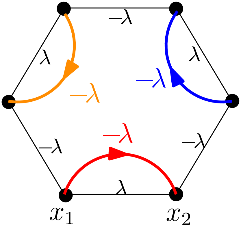
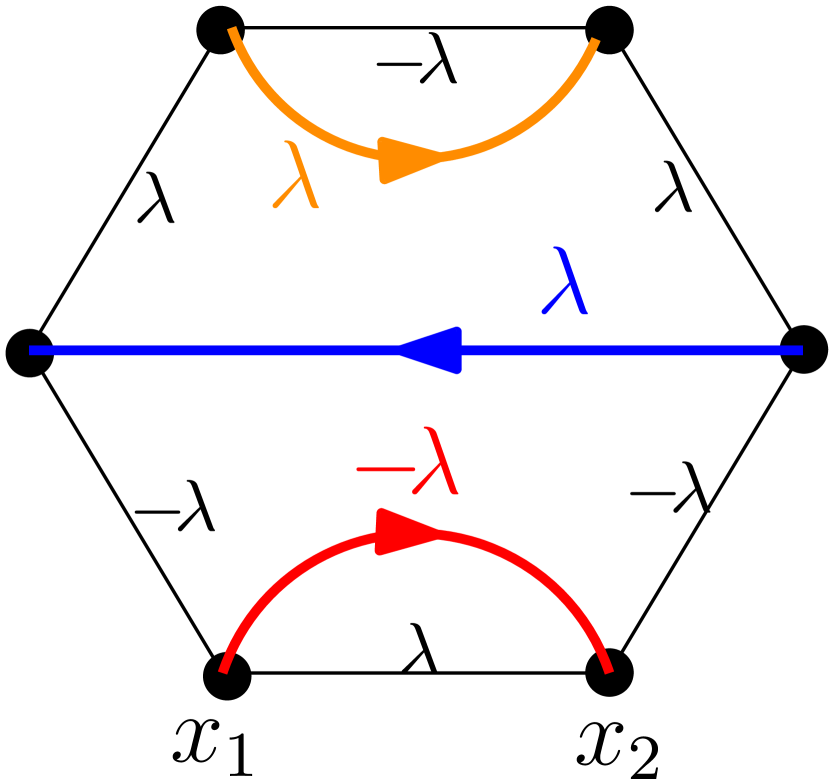
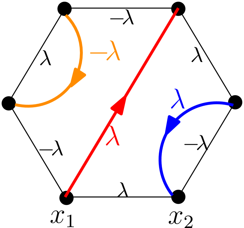
[Degenerate case in Theorem 1.2—level lines of ] When , the SDE (3.1) degenerates to the SDE (2.2). In other words, in with marked points is the same as with force points . In this degenerate case, the pair of curves in Theorem 1.2 can be realized by a pair of level lines of . Fix a quad . Let be the on with the following boundary data: on , on , and on . Let be the level line of with height zero starting from and let be the level line of with height starting from . Then we have that the marginal law of is and the conditional law of given is ; the marginal law of is and the conditional law of given is . Thus the pair is the unique pair described in Theorem 1.2 for .
Furthermore, the case with can be easily generalized to multiple curves. Fix , a simply connected proper subset , and along the boundary of in counterclockwise order. For each planar pair partition of , let be the collection of non-intersecting simple curves such that for . Then there exists a unique probability measure on with the following property: the conditional law of given is process for each .
Moreover, this unique probability measure can be obtained by level lines of . Suppose is a in with alternating boundary conditions: on and on (with the convention that ). For , let be the level line of starting from . Then the end points of form a planar pair partition of , see Figure 4.1. For each planar pair partition of , the probability is strictly positive. Conditioned on the event , the collection of level lines is in , and it has the property that the conditional law of given is the same as the level line of with Dobrushin boundary condition, thus the conditional law is , for all .
4.3 Proof of Proposition 1.4
Lemma 4.5.
Fix a Dobrushin domain and , , and . There exists a unique probability measure on pairs of curves in with the following property: the conditional law of given is and the conditional law of given is . Under this probability measure, the marginal law of is and the marginal law of is .
Proof.
By the argument before the proof of Proposition 4.1, we only need to show the conclusion for . We first show the existence of the pair by checking that a certain pair of flow lines in satisfies the desired property. Suppose is a in with boundary data
Set . Let be the flow line of with angle and be the flow line of with angle . Then one can check that the conditional law of given is and the conditional law of given is ; and that the marginal laws of and are the same as the one in the statement. It remains to show the uniqueness. This can be obtained by reducing to the setting that the end points are distinct—Proposition 4.1. This is explained at the begining of [MS16b, Proof of Theorem 4.1]. ∎
Proof of Proposition 1.4.
We first check that the curves can be realized by flow lines of . Suppose is a on with the boundary data: on and on . Set for . Let be the flow line of with angle . Then one can check that the conditional law of given and is for and the marginal law of is .
We prove the uniqueness by induction on . Lemma 4.5 implies the conclusion for . Suppose the conclusion holds for path and consider . Applying the hypothesis to , we know the conditional law of given . In particular, we know that the conditional law of given is and the conditional law of given is . Thus, by Lemma 4.5, we know that the marginal law of is . The marginal law of and the conditional law of given uniquely determine the law of . This completes the proof. ∎
Remark 4.6.
The conclusions in Proposition 1.4 hold as long as the terminal points of curves coincide. Suppose that are boundary points of in counterclockwise order and denote by the collection of curves where and it is to the right of and is to the left of for with the convention that and . Fix . Then there is a unique probability measure on such that the the conditional law of given and is for . Under this measure, the marginal law of is where each of corresponds to a force point with weight .
5 Ising Model and Proof of Theorem 1.3
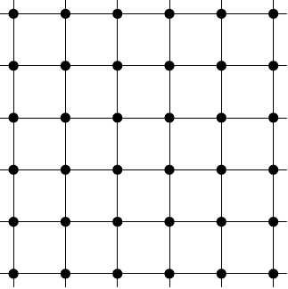
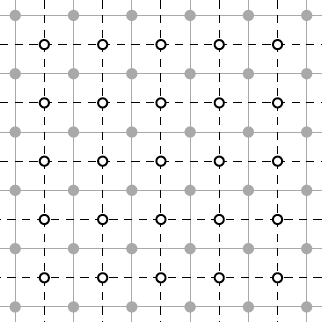
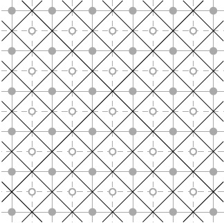
Notations and terminologies. We focus on the square lattice . Two vertices and are neighbors if , and we write . The dual square lattice is the dual graph of . The vertex set is and the edges are given by nearest neighbors. The vertices and edges of are called dual-vertices and dual-edges. In particular, for each edge of , it is associated to a dual edge, denoted by , that it crosses in the middle. For a finite subgraph , we define to be the subgraph of with edge-set and vertex set given by the end-points of these dual-edges. The medial lattice is the graph with the centers of edges of as vertex set, and edges connecting nearest vertices. This lattice is a rotated and rescaled version of , see Figure 5.1. The vertices and edges of are called medial-vertices and medial-edges. We identify the faces of with the vertices of and . A face of is said to be black if it corresponds to a vertex of and white if it corresponds to a vertex of .
5.1 Ising model
Let be a finite subset of . The Ising model with free boundary conditions is a random assignment of spins , where denotes the spin at the vertex . The Hamiltonian of the Ising model is defined by
The Ising measure is the Boltzmann measure with Hamiltonian and inverse-temperature :
For a graph and , one may also define the Ising model with boundary conditions by the Hamiltonian
Ising model satisfies Domain Markov property: Let be two finite subsets of . Let and . Let be a random variable which is measurable with respect to vertices in . Then we have
Suppose that is a Dobrushin domain. The Dobrushin boundary condition is the following: along , and along . This boundary condition is also called domain-wall boundary condition. Suppose that is a quad. The alternating boundary condition is the following: along and , and along and .
The set is equipped with a partial order: if for all . A random variable is increasing if implies . An event is increasing if is increasing. The Ising model satisfies FKG inequality: Let be a finite subset and be boundary conditions, and . For any two increasing events and , we have
As a consequence of FKG inequality, we have the comparison between boundary conditions: For boundary conditions and an increasing event , we have
| (5.1) |
The critical value of in Ising model is given by:
The critical Ising model is conformal invariant in the scaling limit. We will list two special properties for the critical Ising model that will be useful later: strong RSW and the convergence of the interface with Dobrushin boundary condition.
Given a quad on the square lattice, we denote by the discrete extermal distance between and in , see [Che16, Section 6]. The discrete extremal distance is uniformly comparable to and converges to its continuous counterpart— the classical extremal distance. The quad is crossed by in an Ising configuration if there exists a path of going from to in . We denote this event by .
Proposition 5.1.
[CDCH16, Corollary 1.7]. For each there exists such that the following holds: for any quad with ,
where the boundary conditions are on and on .
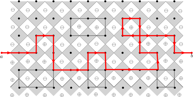
For , we consider the rescaled square lattice . The definitions of dual lattice, medial lattice and Dobrushin domains extend to this context, and they will be denoted by , , respectively. Consider the critical Ising model on . The boundary is divided into two parts and . We fix the Dobrushin boundary conditions: on and on . Define the interface as follows. It starts from , lies on the primal lattice and turns at every vertex of is such a way that it has always dual vertices with spin on its left and on its right. If there is an indetermination when arriving at a vertex (this may happen on the square lattice), turn left. See Figure 5.2. We have the convergence of the interface:
Theorem 5.2.
[CDCH+14]. Let be a family of Dobrushin domains converging to a Dobrushin domain in the Carathéodory sense. The interface of the critical Ising model in with Dobrushin boundary condition converges weakly to as .
Theorem 5.3.
Let be a family of Dobrushin domains converging to a Dobrushin domain in the Carathéodory sense. The interface of the critical Ising model in with the boundary condition along and along converges weakly to as .
5.2 Proof of Theorem 1.3
Let be a sequence of discrete quads on the square lattice approximating some quad . Consider the critical Ising model in with alternating boundary conditions: along and , and along , and along . Suppose there is a vertical crossing of and denote this event by
Let be the interface starting from lying on the primal lattice. It turns at every vertex in the way that it has spin on its left and on its right, and that it turns left when there is ambiguity. Let be the interface starting from lying on the primal lattice. It turns at every vertex in the way that it has spin to its left and to its right, and turns right when there is ambiguity. Then will end at and will end at . See Figure 1.1. Let be the connected component of with on the boundary and denote by the discrete extremal distance between and in . Define and similarly.
Lemma 5.4.
The variables is tight in the following sense: for any , there exists such that
Proof.
Since approximates , by Proposition 5.1 and (5.1), we know that can be bounded from below by some quantity that depends only on the extremal distance in between and and that is uniform over . Thus, it is sufficient to show is small for small. Given and on the event , combining Proposition 5.1 and (5.1), we know that the probability to have a vertical crossing of in is bounded by which only depends on and goes to zero as . Thus . This implies the conclusion. ∎
Proof of Theorem 1.3.
We only prove the conclusion for , and the other cases can be proved similarly (by replacing Theorem 5.2 by 5.3 when necessary). Combining Proposition 5.1 with (5.1) and Lemma 5.4, we see that the sequence satisfies the requirements in Theorem 2.4, thus the sequence is relatively compact. Suppose is any sub-sequential limit and, for some ,
Since , by Theorem 2.2, we know that we have the convergence in all three topologies. In particular, this implies the convergence of in Carathéodory sense. Note that the conditional law of in given is the interface of the critical planar Ising model with Dobrushin boundary condition. Combining with Theorem 5.2, we know that, the conditional law of in given is . By symmetry, the conditional law of in given is . By Theorem 1.2, there exists a unique such measure. Thus it has to be the unique sub-sequential limit. This completes the proof of Theorem 1.3. ∎
6 FK-Ising Model and Proof of Proposition 1.5
6.1 FK-Ising model
We will consider finite subgraphs . For such a graph, we denote by the inner boundary of :
A configuration is an element of . If , the edge is said to be open, otherwise is said to be closed. The configuration can be seen as a subgraph of with the same set of vertices , and the set of edges given by open edges .
We are interested in the connectivity properties of the graph . The maximal connected components of are called clusters. Two vertices and are connected by inside if there exists a path of vertices in such that and is open in for . We denote this event by . If , we simply drop it from the notation. For , set if there exists a vertex of connected in to a vertex in .
Given a finite subgraph , boundary condition is a partition of . Two vertices are wired in if they belong to the same . The graph obtained from the configuration by identifying the wired vertices together in is denoted by . Boundary conditions should be understood informally as encoding how sites are connected outside of . Let and denote the number of open can dual edges of and denote the number of maximal connected components of the graph .
The probability measure of the random cluster model model on with edge-weight , cluster-weight and boundary condition is defined by
where is the normalizing constant to make a probability measure. For , this model is simply Bernoulli bond percolation.
For a configuration on , the boundary conditions induced by are defined by the partition , where and are in the same if and only if there exists an open path in connecting and . We identify the boundary condition induced by with the configuration itself, and denote the random cluster model with these boundary conditions by . As a direct consequence of these definitions, we have the Domain Markov Property of the random cluster model: Suppose that are two finite subgraphs of . Fix and some boundary conditions on . Let be a random variable which is measurable with respect to edges in . Then we have
where is the partition on obtained as follows: two vertices are wired if they are connected in .
Suppose that is a Dobrushin domain. The Dobrushin boundary condition is the following: free along and wired along . Suppose that is a quad. The alternating boundary condition is the following: free along and , wired along and .
Denote the product ordering on by . In other words, for , we denote by if , for all . An event depending on edges in is increasing if for any implies . We have positive association (FKG inequality) when : Fix and a finite graph and some boundary conditions . For any two increasing events and , we have
As a consequence of the FKG inequality, we have the comparison principle between boundary conditions: fix and a finite graph . For any boundary conditions and any increasing event , we have
For a finite subgraph , we define to be the subgraph of with edge-set and vertex set given by the end-points of these dual-edges. A configuration on can be uniquely associated to a dual configuration on the dual graph defined as follows: set for all . A dual-edge is said to be dual-open if , it is dual-closed otherwise. A dual-cluster is a connected component of . We extend the notion of dual-open path and the connective events in the obvious way. If is distributed according to , then is distributed according to where
and the boundary conditions can be deduced from in a case by case manner. In particular, corresponds to and corresponds to .
The critical value of for a given is the following:
People believe that the critical random-cluster model is conformal invariant in the scaling limit for , and it is only proved for in [CS12, CDCH+14]. When , the critical random-cluster model is also called FK-Ising model. We will list two special properties for the FK-Ising model that will be useful later: strong RSW and the convergence of the interface with Dobrushin boundary condition.
Proposition 6.1.
[CDCH16, Theorem 1.1]. For each there exists such that the following holds: for any quad with and for any boundary conditions ,
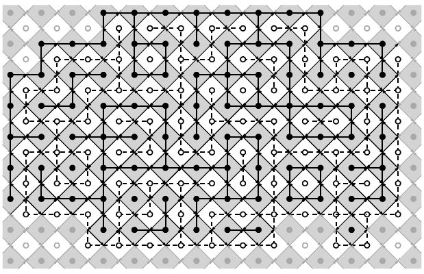
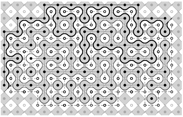
Fix a Dobrushin domain and consider a configuration together with its dual-configuration . The Dobrushin boundary condition is given by taking edges of to be open and the dual-edges of to be dual-open. Through every vertex of , there passes either an open edge of or a dual open edge of . Draw self-avoiding loops on as follows: a loop arriving at a vertex of the medial lattice always makes a turn so as not to cross the open or dual open edges through this vertex, see Figure 6.1. The loop representation contains loops together with a self-avoiding path going from to . This curve is called the exploration path. See [DC13, Section 6.1] for more details.
Theorem 6.2.
[CDCH+14]. Let be a family of Dobrushin domains converging to a Dobrushin domain in the Carathéodory sense. The exploration path of the critical FK-Ising model with Dobrushin boundary conditions converges weakly to as .
6.2 Proof of Proposition 1.5
Lemma 6.3.
Let be a family of quads converging to a quad in the Carathéodory sense. Consider the critical FK-Ising model with Dobrushin boundary condition: wired on and free on and denote by the exploration path from to . Denote by the event that there is a dual-crossing in from to . Then the law of conditioned on the event converges weakly to in from to conditioned not to hit as . Given and on the event , define to be the discrete extremal distance between and in which is the connected component of with on the boundary. Then is tight in the following sense: for any , there exists such that
Proof.
Lemma 6.4.
Let be a sequence of discrete quads on the square lattice approximating some quad . Consider the critical FK-Ising model in with alternating boundary conditions: free on and , and wired on and . Conditioned on the event that there are two disjoint vertical dual-crossings, then there exists a pair of interfaces where (resp. ) is the interface connecting to (resp. connecting to ). The law of converges weakly to the unique pair of curves in with the following property: Given , the conditional law of is an conditioned not to hit ; given , the conditional law of is an conditioned not to hit .
Proof.
Combining Proposition 6.1 and Lemma 6.3, we see that the sequence satisfies the requirements in Theorem 2.4, thus the sequence is relatively compact. Suppose is any subsequential limit and, for some , we have in distribution. Let be the connected component of with on the boundary, and define similarly. Since , combining with Theorem 2.2, we have the convergence in all three topologies. In particular, the quads converges to in Carathéodory sense. Combining with Lemma 6.3, we know that the conditional law of given is conditioned not to hit . By symmetry, the conditional of given is conditioned not to hit . It remains to explain that there is a unique measure on pairs with such property. The uniqueness can be proved by the same argument as in the proof of Proposition 4.1. The key point is that the two curves do not hit each other and that the counterflow line is deterministic function of the and thus the event that the counterflow line does not hit part of the boundary is also deterministic of the . ∎
Proof of Proposition 1.5.
Fix . We derive the conclusion by three steps: first, let the quads approximate some quad ; second, let ; thirdly, let . In the first step, by Lemma 6.4, we know that the pairs of interfaces converge weakly to a unique probability measure on such that the conditional law of given is conditioned not to hit and the conditional law of given is conditioned not to hit . Now, let us fix and let . By Lemma 2.7, we know that the conditional law of given converges weakly to . Let be the collection of pairs of curves such that and that is to the left of . From the above analysis, by sending , the limiting probability measure on satisfies the following property: the conditional law of given is and the conditional law of given is . By Lemma 4.5, there exists a unique such measure, and under this measure, the marginal law of is with force point located at and the marginal law of is with force point located at . Finally, since the law of process is continuous in the locations of the force points, we complete the proof by sending . ∎
Acknowledgment
The author is supported by the NCCR/SwissMAP, the ERC AG COMPASP, the Swiss NSF. The author thanks Dmitry Chelkak and Stanislav Smirnov for helpful discussion about Ising and FK-Ising model with alternating boundary conditions. The author thanks Gregory Lawler for helpful discussion on multiple SLEs.
References
- [AS92] Milton Abramowitz and Irene A. Stegun, editors. Handbook of mathematical functions with formulas, graphs, and mathematical tables. Dover Publications, Inc., New York, 1992. Reprint of the 1972 edition.
- [BBK05] Michel Bauer, Denis Bernard, and Kalle Kytölä. Multiple Schramm-Loewner evolutions and statistical mechanics martingales. J. Stat. Phys., 120(5-6):1125–1163, 2005.
- [BDCH14] Stéphane Benoist, Hugo Duminil-Copin, and Clément Hongler. Conformal invariance of crossing probabilities for the ising model with free boundary conditions. arXiv preprint arXiv:1410.3715, 2014.
- [Bil99] Patrick Billingsley. Convergence of Probability Measures. 1999.
- [CDCH+14] Dmitry Chelkak, Hugo Duminil-Copin, Clément Hongler, Antti Kemppainen, and Stanislav Smirnov. Convergence of ising interfaces to schrammʼs sle curves. Comptes Rendus Mathematique, 352(2):157–161, 2014.
- [CDCH16] Dmitry Chelkak, Hugo Duminil-Copin, and Clément Hongler. Crossing probabilities in topological rectangles for the critical planar FK-Ising model. Electron. J. Probab., 21:Paper No. 5, 28, 2016.
- [Che16] Dmitry Chelkak. Robust discrete complex analysis: A toolbox. The Annals of Probability, 44(1):628–683, 2016.
- [CS12] Dmitry Chelkak and Stanislav Smirnov. Universality in the 2D Ising model and conformal invariance of fermionic observables. Invent. Math., 189(3):515–580, 2012.
- [DC13] Hugo Duminil-Copin. Parafermionic observables and their applications to planar statistical physics models. Ensaios Matematicos, 25:1–371, 2013.
- [Dub05] Julien Dubédat. martingales and duality. Ann. Probab., 33(1):223–243, 2005.
- [Dub07] Julien Dubédat. Commutation relations for Schramm-Loewner evolutions. Comm. Pure Appl. Math., 60(12):1792–1847, 2007.
- [Dub09] Julien Dubédat. Duality of Schramm-Loewner evolutions. Ann. Sci. Éc. Norm. Supér. (4), 42(5):697–724, 2009.
- [HK13] Clément Hongler and Kalle Kytölä. Ising interfaces and free boundary conditions. Journal of the American Mathematical Society, 26(4):1107–1189, 2013.
- [Izy13] Konstantin Izyurov. Critical ising interfaces in multiply-connected domains, 2013.
- [Izy15] Konstantin Izyurov. Smirnov’s observable for free boundary conditions, interfaces and crossing probabilities. Comm. Math. Phys., 337(1):225–252, 2015.
- [KL07] Michael J. Kozdron and Gregory F. Lawler. The configurational measure on mutually avoiding SLE paths. In Universality and renormalization, volume 50 of Fields Inst. Commun., pages 199–224. Amer. Math. Soc., Providence, RI, 2007.
- [KP16] Kalle Kytölä and Eveliina Peltola. Pure partition functions of multiple SLEs. Comm. Math. Phys., 346(1):237–292, 2016.
- [KS12] Antti Kemppainen and Stanislav Smirnov. Random curves, scaling limits and loewner evolutions. arXiv preprint arXiv:1212.6215, 2012.
- [Law09] Gregory F. Lawler. Partition functions, loop measure, and versions of SLE. J. Stat. Phys., 134(5-6):813–837, 2009.
- [LSW03] Gregory F. Lawler, Oded Schramm, and Wendelin Werner. Conformal restriction: the chordal case. J. Amer. Math. Soc., 16(4):917–955 (electronic), 2003.
- [LW04] Gregory F. Lawler and Wendelin Werner. The Brownian loop soup. Probab. Theory Related Fields, 128(4):565–588, 2004.
- [MS16a] Jason Miller and Scott Sheffield. Imaginary geometry I: interacting SLEs. Probab. Theory Related Fields, 164(3-4):553–705, 2016.
- [MS16b] Jason Miller and Scott Sheffield. Imaginary geometry II: Reversibility of for . Ann. Probab., 44(3):1647–1722, 2016.
- [MS16c] Jason Miller and Scott Sheffield. Imaginary geometry III: reversibility of for . Ann. of Math. (2), 184(2):455–486, 2016.
- [Phe01] Robert R. Phelps. Lectures on Choquet’s theorem, volume 1757 of Lecture Notes in Mathematics. Springer-Verlag, Berlin, second edition, 2001.
- [Qia16] Wei Qian. Conformal restriction: The trichordal case, 2016.
- [RS05] Steffen Rohde and Oded Schramm. Basic properties of SLE. Ann. of Math. (2), 161(2):883–924, 2005.
- [SS13] Oded Schramm and Scott Sheffield. A contour line of the continuum Gaussian free field. Probab. Theory Related Fields, 157(1-2):47–80, 2013.
- [SW05] Oded Schramm and David B. Wilson. SLE coordinate changes. New York J. Math., 11:659–669 (electronic), 2005.
- [WW13] Wendelin Werner and Hao Wu. From CLE() to SLE(). Electron. J. Probab., 18:no. 36, 1–20, 2013.
- [WW16] Menglu Wang and Hao Wu. Level Lines of Gaussian Free Field I: Zero-Boundary GFF. Stochastic Processes and their Applications, page to appear, 2016.
- [Zha08] Dapeng Zhan. Reversibility of chordal SLE. Ann. Probab., 36(4):1472–1494, 2008.