Computational mechanics of soft filaments

Mattia Gazzola Department of Mechanical Science and Engineering, National Center for Supercomputing Applications, University of Illinois at Urbana-Champaign, Urbana, IL 61801, USA    Levi H. Dudte John A. Paulson School of Engineering and Applied Sciences, Harvard University, Cambridge, MA 02138, USA    Andrew G. McCormick Google, Mountain View, CA 94043, USA John A. Paulson School of Engineering and Applied Sciences, Harvard University, Cambridge, MA 02138, USA    L. Mahadevan lm@seas.harvard.edu John A. Paulson School of Engineering and Applied Sciences, and Department of Physics, Harvard University, Cambridge, MA 02138, USA
Abstract

Soft slender structures are ubiquitous in natural and artificial systems and can be observed at scales that range from the nanometric to the kilometric, from polymers to space tethers. We present a practical numerical approach to simulate the dynamics of filaments that, at every cross-section, can undergo all six possible modes of deformation, allowing the filament to bend, twist, stretch and shear, while interacting with complex environments via muscular activity, surface contact, friction and hydrodynamics. We examine the accuracy of our method by means of several benchmark problems with known analytic solutions. We then demonstrate the capabilities and robustness of our approach to solve forward problems in physics and mechanics related to solenoid and plectoneme formation in twisted, stretched filaments, and inverse problems related to active biophysics of limbless locomotion on solid surfaces and in bulk liquids. All together, our approach provides a robust computational framework to characterize the mechanical response and design of soft active slender structures.

I Introduction

Quasi one-dimensional objects are characterized by having one dimension, the length L𝐿L, much larger than the others, say the radius r𝑟r, so that L/r1much-greater-than𝐿𝑟1L/r\gg 1. Relative to three-dimensional objects, this measure of slenderness allows for significant mathematical simplification in accurately describing the physical dynamics of strings, filaments and rods. It is thus perhaps not surprising that the physics of strings has been the subject of intense study for centuries Kirchhoff:1859 ; Clebsch:1883 ; Love:1906 ; Cosserat:1909 ; Antman:1973 ; Dill:1992 ; Langer:1996 ; vanDerHeijden:2000 ; Goss:2005 ; Maugin:2010 , and indeed their investigation substantially pre-dates the birth of three-dimensional elasticity.

Following the pioneering work of Galileo on the bending of cantilevers, one-dimensional analytical models of beams date back to 1761 when Jakob Bernoulli first introduced the use of differential equations to capture the relation between geometry and bending resistance in a planar elastica, that is an elastic curve deforming in a two-dimensional space. This attempt was then progressively refined by Huygens, Leibniz and Johann Bernoulli Goss:2009 , until Euler presented a full solution of the planar elastica, obtained by minimizing the strain energy and by recognizing the relation between flexural stiffness and material and geometric properties. Euler also showed the existence of bifurcating solutions in a rod subject to compression, identifying its first buckling mode, while Lagrange formalized the corresponding multi-modal solution Antman:1973 . Non-planar deformations of the elastica were first tackled by Kirchhoff Kirchhoff:1859 ; Dill:1992 and Clebsch Clebsch:1883 who envisioned a rod as an assembly of short undeformable straight segments with dynamics determined by contact forces and moments, leading to three-dimensional configurations. Later, Love Love:1906 approached the problem from a Lagrangian perspective characterizing a filament by contiguous cross sections that can rotate relative to each other, but remain undeformed and perpendicular to the centerline of the rod at all times; in modern parlance this assumption is associated with dynamics on the rotation group SO(3) at every cross-section. The corresponding equations of motion capture the ability of the filament to bend and twist, but not shear or stretch. Eventually the Cosserat brothers Cosserat:1909 relaxed the assumption of inextensibility and cross-section orthogonality to the centerline, deriving a general mathematical framework that accommodates all six possible degrees of freedom associated with bending, twisting, stretching and shearing, effectively formulating dynamics on the full Euclidean group SE(3).

The availability of these strong mathematical foundations Antman:1973 prompted a number of discrete computational models Yang:1993 ; Spillmann:2007 ; Bergou:2008 ; Arne:2010 ; Audoly:2013 that allow for the exploration of a range of physical phenomena. These include, for example, the study of polymers and DNA Yang:1993 ; Wolgemuth:2000 , elastic and viscous threads Bergou:2010 ; Arne:2010 ; Audoly:2013 ; Brun:2015 , botanical applications Goriely:1998 ; Gerbode:2012 , elastic ribbons Bergou:2008 , woven cloth Kaldor:2008 and tangled hair Ward:2007 . Because the scaled ratio of the stretching and shearing stiffness to the bending stiffness for slender filaments is L2/r21much-greater-thansuperscript𝐿2superscript𝑟21L^{2}/r^{2}\gg 1, the assumption of inextensibility and unshearability is usually appropriate, justifying the widespread use of the Kirchhoff model in the aforementioned applications.

However, new technologies such as soft robotics and artificial muscles Kim:2013 ; Haines:2014 ; Park:2016 are generating applications for deformable and stretchable elastomeric filamentous structures Haines:2014 for which the assumption of inextensibility and unshearability is no longer valid. Motivated by these advancements, we move away from the Kirchhoff model in favor of the complete Cosserat theory. We present a robust and relatively simple numerical scheme that tracks both the rod centerline and local frame allowing for bend, twist, stretch and shear Cosserat:1909 consistent with the full Euclidean group SE(3), while retaining the Hamiltonian structure of the system and fast discrete operators. This allows us to substantially increase the spectrum of problems amenable to be treated via this class of rod models.

Moving beyond the passive mechanics of individual filaments, we also account for the interaction between filaments and complex environments with a number of additional biological and physical features, including muscular activity, self-contact and contact with solid boundaries, isotropic and anisotropic surface friction and viscous interaction with a fluid. Finally, we demonstrate the capabilities and the robustness of our solver by embedding it in an inverse design cycle for the identification of optimal terrestrial and aquatic limbless locomotion strategies.

The paper is structured as follows. In Section II we review and introduce the mathematical foundations of the model. In Section III we present the corresponding discrete scheme and validate our framework against a battery of benchmark problems. In Section IV we detail the physical and biological enhancements to the original model, and finally in Section V we showcase the potential of our solver via the study of solenoids and plectonemes as well as limbless biolocomotion. Mathematical derivations and additional validation test cases are presented in the Appendix.

II Governing Equations

We consider filaments as slender cylindrical structures deforming in three-dimensions with a characteristic length L𝐿L which is assumed to be much larger than the radius (Lrmuch-greater-than𝐿𝑟L\gg r) at any cross section. Then the filament can be geometrically reduced to a one-dimensional representation, and its dynamical behavior may be approximated by averaging all balance laws at every cross section Antman:1973 . We start with a description of the commonly used Kirchhoff-Love theory that accounts for bend and twist at every cross-section but ignores stretch and shear, before moving on to the Cosserat theory that accounts for these additional degrees of freedom as well.

II.1 Kirchhoff-Love theory for inextensible, unshearable rods
Refer to caption
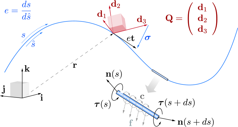
Figure 1: The Cosserat rod model. A filament deforming in the three-dimensional space is represented by a centerline coordinate 𝐫𝐫\mathbf{r} and a material frame characterized by the orthonormal triad {𝐝1,𝐝2,𝐝3}subscript𝐝1subscript𝐝2subscript𝐝3\{\mathbf{d}_{1},\mathbf{d}_{2},\mathbf{d}_{3}\}. The corresponding orthogonal rotation matrix 𝐐𝐐\mathbf{Q} with row entries 𝐝1subscript𝐝1\mathbf{d}_{1}, 𝐝2subscript𝐝2\mathbf{d}_{2}, 𝐝3subscript𝐝3\mathbf{d}_{3} transforms a vector 𝐱𝐱\mathbf{x} from the laboratory canonical basis {𝐢,𝐣,𝐤}𝐢𝐣𝐤\{\mathbf{i},\mathbf{j},\mathbf{k}\} to the material frame of reference {𝐝1,𝐝2,𝐝3}subscript𝐝1subscript𝐝2subscript𝐝3\{\mathbf{d}_{1},\mathbf{d}_{2},\mathbf{d}_{3}\} so that 𝐱=𝐐𝐱subscript𝐱𝐐𝐱\mathbf{x}_{\mathcal{L}}=\mathbf{Q}\mathbf{x} and vice versa 𝐱=𝐐T𝐱𝐱superscript𝐐𝑇subscript𝐱\mathbf{x}=\mathbf{Q}^{T}\mathbf{x}_{\mathcal{L}}. If extension or compression is allowed, the current filament configuration arc-length s𝑠s may no longer coincide with the rest reference arc-length s^^𝑠\hat{s}. This is captured via the scalar dilatation field e=ds/ds^𝑒𝑑𝑠𝑑^𝑠e=ds/d\hat{s}. Moreover, to account for shear we allow the triad {𝐝1,𝐝2,𝐝3}subscript𝐝1subscript𝐝2subscript𝐝3\{\mathbf{d}_{1},\mathbf{d}_{2},\mathbf{d}_{3}\} to detach from the unit tangent vector 𝐭𝐭\mathbf{t} so that 𝐝3𝐭subscript𝐝3𝐭\mathbf{d}_{3}\neq\mathbf{t} (we recall that the condition 𝐝3=𝐭subscript𝐝3𝐭\mathbf{d}_{3}=\mathbf{t} and e=1𝑒1e=1 correspond to the Kirchhoff constraint for unshearable and inextensible rods, and implies that 𝝈=e𝐭𝐝3=𝟎𝝈𝑒𝐭subscript𝐝30\boldsymbol{\sigma}=e\mathbf{t}-\mathbf{d}_{3}=\mathbf{0}). The dynamics of centerline and material frame are related through quadratic energy functionals that give rise at each cross section to the internal force and torque resultants, 𝐧𝐧\mathbf{n} and 𝝉𝝉\boldsymbol{\tau}. External loads are represented via the force 𝐟𝐟\mathbf{f} and couple 𝐜𝐜\mathbf{c} line densities.

As illustrated in Fig. 1, a filament in the Cosserat rod theory can be described by a centerline 𝐫:(s[0,L],t+)3\mathbf{r}:(s\in[0,L]\in\mathbb{R},t\in\mathbb{R}^{+})\rightarrow\mathbb{R}^{3} and an oriented frame of reference 𝐐:(s[0,L],t+)SO(3)\mathbf{Q}:(s\in[0,L]\in\mathbb{R},t\in\mathbb{R}^{+})\rightarrow\text{SO}(3) equivalent to the orthonormal triad of unit vectors 𝐐={𝐝1,𝐝2,𝐝3}𝐐subscript𝐝1subscript𝐝2subscript𝐝3\mathbf{Q}=\{\mathbf{d}_{1},\mathbf{d}_{2},\mathbf{d}_{3}\}. Here, s𝑠s is the centerline arc-length coordinate in its current configuration and t𝑡t is time.

Denoting by 𝐱𝐱\mathbf{x} any generic vector represented in the Eulerian frame and 𝐱subscript𝐱\mathbf{x}_{\mathcal{L}} as the body-convected (Lagrangian) frame of reference allows us to write

laboratory: 𝐱=x¯1𝐢+x¯2𝐣+x¯3𝐤,𝐱subscript¯𝑥1𝐢subscript¯𝑥2𝐣subscript¯𝑥3𝐤\displaystyle~{}~{}~{}~{}\mathbf{x}=\bar{x}_{1}\mathbf{i}+\bar{x}_{2}\mathbf{j}+\bar{x}_{3}\mathbf{k}, (1)
body-convected: 𝐱=x1𝐝1+x2𝐝2+x3𝐝3,subscript𝐱subscript𝑥1subscript𝐝1subscript𝑥2subscript𝐝2subscript𝑥3subscript𝐝3\displaystyle~{}~{}~{}~{}\mathbf{x}_{\mathcal{L}}=x_{1}\mathbf{d}_{1}+x_{2}\mathbf{d}_{2}+x_{3}\mathbf{d}_{3}, (2)

where Eq. (1) expresses 𝐱𝐱\mathbf{x} in the laboratory canonical basis {𝐢,𝐣,𝐤}𝐢𝐣𝐤\{\mathbf{i},\mathbf{j},\mathbf{k}\}, while Eq. (2) expresses the same vector in the body-convected director basis {𝐝1,𝐝2,𝐝3}subscript𝐝1subscript𝐝2subscript𝐝3\{\mathbf{d}_{1},\mathbf{d}_{2},\mathbf{d}_{3}\}. Then, the matrix 𝐐𝐐\mathbf{Q} transforms any vector 𝐱𝐱\mathbf{x} from the laboratory to the body-convected representation via 𝐱=𝐐𝐱subscript𝐱𝐐𝐱\mathbf{x}_{\mathcal{L}}=\mathbf{Q}\mathbf{x} and conversely, 𝐱=𝐐1𝐱=𝐐T𝐱𝐱superscript𝐐1subscript𝐱superscript𝐐𝑇subscript𝐱\mathbf{x}=\mathbf{Q}^{-1}\mathbf{x}_{\mathcal{L}}=\mathbf{Q}^{T}\mathbf{x}_{\mathcal{L}}, since 𝐐T𝐐=𝐐𝐐T=𝟏superscript𝐐𝑇𝐐superscript𝐐𝐐𝑇1\mathbf{Q}^{T}\mathbf{Q}=\mathbf{Q}\mathbf{Q}^{T}=\boldsymbol{1}. In general we need to distinguish between the arc-length coordinate s𝑠s that corresponds to the current filament configuration and the arc-length coordinate s^^𝑠\hat{s} associated with the reference configuration of the filament, due to stretching (Fig. 1 (throughout we will use hatted quantities to denote the reference configuration).

We will first start by presenting the equations of motion under the assumption of inextensibility (i.e. s=s^𝑠^𝑠s=\hat{s}), before generalizing them to the stretchable case in the subsequent sections. Denoting the rod angular velocity as 𝝎=vec[𝐐tT𝐐]𝝎vecdelimited-[]superscript𝐐𝑡𝑇𝐐\boldsymbol{\omega}={\rm vec}[\frac{\partial\mathbf{Q}}{\partial t}^{T}\mathbf{Q}] and the generalized curvature as 𝜿=vec[𝐐sT𝐐]𝜿vecdelimited-[]superscript𝐐𝑠𝑇𝐐\boldsymbol{\kappa}={\rm vec}[\frac{\partial\mathbf{Q}}{\partial s}^{T}\mathbf{Q}], where vec[𝐀]vecdelimited-[]𝐀\rm vec[\mathbf{A}] denotes the 3-vector associated with the skew-symmetric matrix 𝐀𝐀\mathbf{A}, the following transport identities hold

𝐐𝐱t=𝐱t+𝝎×𝐱,𝐐𝐱s=𝐱s+𝜿×𝐱.formulae-sequence𝐐𝐱𝑡subscript𝐱𝑡subscript𝝎subscript𝐱𝐐𝐱𝑠subscript𝐱𝑠subscript𝜿subscript𝐱\mathbf{Q}\frac{\partial\mathbf{x}}{\partial t}=\frac{\partial\mathbf{x}_{\mathcal{L}}}{\partial t}+\boldsymbol{\omega}_{\mathcal{L}}\times\mathbf{x}_{\mathcal{L}},~{}~{}~{}~{}~{}~{}~{}~{}~{}~{}~{}~{}~{}~{}\mathbf{Q}\frac{\partial\mathbf{x}}{\partial s}=\frac{\partial\mathbf{x}_{\mathcal{L}}}{\partial s}+\boldsymbol{\kappa}_{\mathcal{L}}\times\mathbf{x}_{\mathcal{L}}. (3)

Using the above equations (full derivation in the Appendix) we can express the advection of the rod positions and local frames, as well as the linear and angular momentum balance in a convenient Eulerian-Lagrangian form

𝐫t𝐫𝑡\displaystyle\frac{\partial\mathbf{r}}{\partial t} =\displaystyle= 𝐯𝐯\displaystyle\mathbf{v} (4)
𝐝jtsubscript𝐝𝑗𝑡\displaystyle\frac{\partial\mathbf{d}_{j}}{\partial t} =\displaystyle= (𝐐T𝝎)×𝐝j,j=1,2,3formulae-sequencesuperscript𝐐𝑇subscript𝝎subscript𝐝𝑗𝑗123\displaystyle(\mathbf{Q}^{T}\boldsymbol{\omega}_{\mathcal{L}})\times\mathbf{d}_{j},~{}~{}~{}~{}~{}j=1,2,3 (5)
(ρA𝐯)t𝜌𝐴𝐯𝑡\displaystyle\frac{\partial(\rho A\mathbf{v})}{\partial t} =\displaystyle= (𝐐T𝐧)s+𝐟superscript𝐐𝑇subscript𝐧𝑠𝐟\displaystyle\frac{\partial(\mathbf{Q}^{T}\mathbf{n}_{\mathcal{L}})}{\partial s}+\mathbf{f} (6)
(ρ𝐈𝝎)t𝜌𝐈subscript𝝎𝑡\displaystyle\frac{\partial(\rho\mathbf{I}\boldsymbol{\omega}_{\mathcal{L}})}{\partial t} =\displaystyle= 𝝉s+𝜿×𝝉+𝐐𝐫s×𝐧+(ρ𝐈𝝎)×𝝎+𝐜,subscript𝝉𝑠subscript𝜿subscript𝝉𝐐𝐫𝑠subscript𝐧𝜌𝐈subscript𝝎subscript𝝎subscript𝐜\displaystyle\frac{\partial\boldsymbol{\tau}_{\mathcal{L}}}{\partial s}+\boldsymbol{\kappa}_{\mathcal{L}}\times\boldsymbol{\tau}_{\mathcal{L}}+\mathbf{Q}\frac{\partial\mathbf{r}}{\partial s}\times\mathbf{n}_{\mathcal{L}}+(\rho\mathbf{I}\boldsymbol{\omega}_{\mathcal{L}})\times\boldsymbol{\omega}_{\mathcal{L}}+\mathbf{c}_{\mathcal{L}}, (7)

where ρ𝜌\rho is the constant material density, A𝐴A is the cross sectional area, 𝐯𝐯\mathbf{v} is the velocity, 𝐧subscript𝐧\mathbf{n}_{\mathcal{L}} and 𝝉subscript𝝉\boldsymbol{\tau}_{\mathcal{L}} are respectively the internal force and couple resultants, 𝐟𝐟\mathbf{f} and 𝐜𝐜\mathbf{c} are external body force and torque line densities, and the tensor 𝐈𝐈\mathbf{I} is the second area moment of inertia (throughout this study we assume circular cross sections, see Appendix).

To close the above system of equations, Eqs. (4-7) and determine the dynamics of the rod, it is necessary to specify the form of the internal forces and torques generated in response to bend and twist, corresponding to the three degrees of freedom at every cross-section. The strains are defined as the relative local deformations of the rod with respect to its natural strain-free reference configuration. Bending and twisting strains are associated with the spatial derivatives of the material frame director field {𝐝1,𝐝2,𝐝3}subscript𝐝1subscript𝐝2subscript𝐝3\{\mathbf{d}_{1},\mathbf{d}_{2},\mathbf{d}_{3}\} and are characterized by the generalized curvature. Specifically, the components of the curvature projected along the directors (𝜿=κ1𝐝1+κ2𝐝2+κ3𝐝3subscript𝜿subscript𝜅1subscript𝐝1subscript𝜅2subscript𝐝2subscript𝜅3subscript𝐝3\boldsymbol{\kappa}_{\mathcal{L}}=\kappa_{1}\mathbf{d}_{1}+\kappa_{2}\mathbf{d}_{2}+\kappa_{3}\mathbf{d}_{3}) coincides with bending (κ1,κ2subscript𝜅1subscript𝜅2\kappa_{1},\kappa_{2}) and twist (κ3subscript𝜅3\kappa_{3}) strains in the material frame (Table 1).

Assuming a linear material constitutive law implies linear stress-strain relations. Integration of the torque densities over the cross sectional area A𝐴A yields the bending and twist rigidities (Table 1), so that the resultant torque-curvature relations can be generically expressed in vectorial notation as

𝝉=𝐁(𝜿𝜿o),subscript𝝉𝐁subscript𝜿subscriptsuperscript𝜿𝑜\boldsymbol{\tau}_{\mathcal{L}}=\mathbf{B}\left(\boldsymbol{\kappa}_{\mathcal{L}}-\boldsymbol{\kappa}^{o}_{\mathcal{L}}\right),~{}~{}~{}~{}~{}~{}~{}~{}~{}~{} (8)

where 𝐁3×3=diag𝐁superscript33diag\mathbf{B}\in\mathbb{R}^{3\times 3}=\text{diag}(B1subscript𝐵1B_{1}, B2subscript𝐵2B_{2}, B3subscript𝐵3B_{3}) is the bend/twist stiffness matrix with B1subscript𝐵1B_{1} the flexural rigidity about 𝐝1subscript𝐝1\mathbf{d}_{1}, B2subscript𝐵2B_{2} the flexural rigidity about 𝐝2subscript𝐝2\mathbf{d}_{2}, B3subscript𝐵3B_{3} the twist rigidity about 𝐝3subscript𝐝3\mathbf{d}_{3}. Here, the vector 𝜿osubscriptsuperscript𝜿𝑜\boldsymbol{\kappa}^{o}_{\mathcal{L}} characterizes the intrinsic curvatures of a filament that in its stress-free state is not straight. We wish to emphasize here that the constitutive laws are most simply expressed in a local Lagrangian form; hence the use of 𝜿subscript𝜿\boldsymbol{\kappa}_{\mathcal{L}} and not 𝜿𝜿\boldsymbol{\kappa}.

The Kirchhoff rod is defined by the additional assumptions that there is no axial extension or compression or shear strain. Then the arc-length s𝑠s coincides with s^^𝑠\hat{s} at all times, and the tangent to the centerline is also normal to the cross-section, so that 𝐭=𝐝3𝐭subscript𝐝3\mathbf{t}=\mathbf{d}_{3} Antman:1973 . This implies that 𝐧subscript𝐧\mathbf{n}_{\mathcal{L}} serves as a Lagrange multiplier, and that the torque-curvature relations of Eq. 8 are linear.

This completes the formulation of the equations of motion for the Kirchhoff rod, and when combined with boundary conditions suffices to have a well-posed initial boundary value problem. For the general stretchable and shearable case, all geometric quantities (A, 𝐈𝐈\mathbf{I}, 𝜿subscript𝜿\boldsymbol{\kappa}_{\mathcal{L}}, etc.) must be rescaled appropriately, as addressed in the following sections.

II.2 Cosserat theory of stretchable and shearable filaments

In the general case of soft filaments, at every cross-section we also wish to capture transverse shear and axial strains in addition to bending and twisting. Since we wish to account for all six deformation modes associated with the six degrees of freedom at each cross section along the rod, we must augment the Kirchhoff description in the previous section and add three more constitutive laws to define the local stress resultants 𝐧subscript𝐧\mathbf{n}_{\mathcal{L}}. In fact, they are no longer defined as Lagrange multipliers that enforce the condition that normals to the cross-section coincide with tangents to the centerline, i.e. we now must have 𝐭𝐝3𝐭subscript𝐝3\mathbf{t}\neq\mathbf{d}_{3}.

The shear and axial strains are associated with the deviations between the unit vector perpendicular to the cross-section and the tangent to the centerline, and thus may be expressed in terms of the derivatives of the centerline coordinate 𝐫𝐫\mathbf{r}. In the material frame of reference, we characterize these strains by the vector 𝝈𝝈\boldsymbol{\sigma} (Fig. 1) which then takes the form

𝝈=𝐐(𝐫s^𝐝3)=𝐐(e𝐭𝐝3).subscript𝝈𝐐𝐫^𝑠subscript𝐝3𝐐𝑒𝐭subscript𝐝3\boldsymbol{\sigma}_{\mathcal{L}}=\mathbf{Q}\left(\frac{\partial\mathbf{r}}{\partial\hat{s}}-\mathbf{d}_{3}\right)=\mathbf{Q}(e\mathbf{t}-\mathbf{d}_{3}). (9)

Here, the scalar field e(s^,t)=ds/ds^𝑒^𝑠𝑡𝑑𝑠𝑑^𝑠e(\hat{s},t)=ds/d\hat{s} expresses the local stretching or compression ratio (Fig. 1) relative to the rest reference configuration (s^^𝑠\hat{s}) and 𝐭𝐭\mathbf{t} is the unit tangent vector.

Whenever the filament undergoes axial stretching or compression the corresponding infinitesimal elements deform and all related geometric quantities are affected. By assuming that the material is incompressible and that the cross sections retain their circular shapes at all times, we can conveniently express the governing equations with respect to the rest reference configuration of the filament (denoted by a hat) in terms of the local dilatation e(s^,t)𝑒^𝑠𝑡e(\hat{s},t). Then, the following relations hold

ds=eds^,A=A^e,𝐈=𝐈^e2,𝐁=𝐁^e2,𝐒=𝐒^e,𝜿=𝜿^e.formulae-sequence𝑑𝑠𝑒𝑑^𝑠formulae-sequence𝐴^𝐴𝑒formulae-sequence𝐈^𝐈superscript𝑒2formulae-sequence𝐁^𝐁superscript𝑒2formulae-sequence𝐒^𝐒𝑒subscript𝜿subscript^𝜿𝑒ds=e\cdot d\hat{s},~{}~{}~{}~{}~{}A=\frac{\hat{A}}{e},~{}~{}~{}~{}~{}\mathbf{I}=\frac{\hat{\mathbf{I}}}{e^{2}},~{}~{}~{}~{}~{}\mathbf{B}=\frac{\hat{\mathbf{B}}}{e^{2}},~{}~{}~{}~{}~{}\mathbf{S}=\frac{\hat{\mathbf{S}}}{e},~{}~{}~{}~{}~{}\boldsymbol{\kappa}_{\mathcal{L}}=\frac{\hat{\boldsymbol{\kappa}}_{\mathcal{L}}}{e}. (10)
deformation modes   strains   rigidities   loads
bending about 𝐝1subscript𝐝1\mathbf{d}_{1}   κ1subscript𝜅1\kappa_{1}   B1=EI1subscript𝐵1𝐸subscript𝐼1B_{1}=EI_{1}   τ1=B1(κ1κ1o)subscript𝜏1subscript𝐵1subscript𝜅1subscriptsuperscript𝜅𝑜1\tau_{1}=B_{1}(\kappa_{1}-\kappa^{o}_{1})
bending about 𝐝2subscript𝐝2\mathbf{d}_{2}   κ2subscript𝜅2\kappa_{2}   B2=EI2subscript𝐵2𝐸subscript𝐼2B_{2}=EI_{2}   τ2=B2(κ2κ2o)subscript𝜏2subscript𝐵2subscript𝜅2subscriptsuperscript𝜅𝑜2\tau_{2}=B_{2}(\kappa_{2}-\kappa^{o}_{2})
twist about 𝐝3subscript𝐝3\mathbf{d}_{3}   κ3subscript𝜅3\kappa_{3}   B3=GI3subscript𝐵3𝐺subscript𝐼3B_{3}=GI_{3}   τ3=B3(κ3κ3o)subscript𝜏3subscript𝐵3subscript𝜅3subscriptsuperscript𝜅𝑜3\tau_{3}=B_{3}(\kappa_{3}-\kappa^{o}_{3})
shear along 𝐝1subscript𝐝1\mathbf{d}_{1}   σ1subscript𝜎1\sigma_{1}   S1=αcGAsubscript𝑆1subscript𝛼𝑐𝐺𝐴S_{1}=\alpha_{c}GA   n1=S1(σ1σ1o)subscript𝑛1subscript𝑆1subscript𝜎1subscriptsuperscript𝜎𝑜1n_{1}=S_{1}(\sigma_{1}-\sigma^{o}_{1})
shear along 𝐝2subscript𝐝2\mathbf{d}_{2}   σ2subscript𝜎2\sigma_{2}   S2=αcGAsubscript𝑆2subscript𝛼𝑐𝐺𝐴S_{2}=\alpha_{c}GA   n2=S2(σ2σ2o)subscript𝑛2subscript𝑆2subscript𝜎2subscriptsuperscript𝜎𝑜2n_{2}=S_{2}(\sigma_{2}-\sigma^{o}_{2})
stretch along 𝐝3subscript𝐝3\mathbf{d}_{3}   σ3subscript𝜎3\sigma_{3}   S3=EAsubscript𝑆3𝐸𝐴S_{3}=EA   n3=S3(σ3σ3o)subscript𝑛3subscript𝑆3subscript𝜎3subscriptsuperscript𝜎𝑜3n_{3}=S_{3}(\sigma_{3}-\sigma^{o}_{3})
Table 1: Constitutive laws. The generalized curvature 𝜿subscript𝜿\boldsymbol{\kappa}_{\mathcal{L}} is associated with the bending κ1subscript𝜅1\kappa_{1}, κ2subscript𝜅2\kappa_{2} about the principal directions (𝐝1subscript𝐝1\mathbf{d}_{1}, 𝐝2subscript𝐝2\mathbf{d}_{2}) and the twist κ3subscript𝜅3\kappa_{3} about the longitudinal one (𝐝3subscript𝐝3\mathbf{d}_{3}), while 𝝈=𝐐(e𝐭𝐝3)subscript𝝈𝐐𝑒𝐭subscript𝐝3\boldsymbol{\sigma}_{\mathcal{L}}=\mathbf{Q}(e\mathbf{t}-\mathbf{d}_{3}) is associated with the shears σ1subscript𝜎1\sigma_{1}, σ2subscript𝜎2\sigma_{2} along the principal directions (𝐝1subscript𝐝1\mathbf{d}_{1}, 𝐝2subscript𝐝2\mathbf{d}_{2}) and the axial extensional or compression σ3subscript𝜎3\sigma_{3} along the longitudinal one (𝐝3subscript𝐝3\mathbf{d}_{3}). The material properties of the rod are captured through the Young’s (E𝐸E) and shear (G) moduli, while its geometric properties are accounted for via the cross sectional area A𝐴A, the second moment of inertia 𝐈𝐈\mathbf{I} and the constant αc=4/3subscript𝛼𝑐43\alpha_{c}=4/3 for circular cross sections Gere:2001 . The diagonal entries of the bending/twist 𝐁3×3𝐁superscript33\mathbf{B}\in\mathbb{R}^{3\times 3} and shear/stretch 𝐒3×3𝐒superscript33\mathbf{S}\in\mathbb{R}^{3\times 3} matrices are, respectively, (B1subscript𝐵1B_{1}, B2subscript𝐵2B_{2}, B3subscript𝐵3B_{3}) and (S1subscript𝑆1S_{1}, S2subscript𝑆2S_{2}, S3subscript𝑆3S_{3}). Pre-strains are modeled via the intrinsic curvature/twist 𝜿osubscriptsuperscript𝜿𝑜\boldsymbol{\kappa}^{o}_{\mathcal{L}} and shear/stretch 𝝈osubscriptsuperscript𝝈𝑜\boldsymbol{\sigma}^{o}_{\mathcal{L}}.

As with the Kirchhoff rod, assuming a linear material constitutive law implies linear stress-strain relations. Integration of the stress and couple densities over the cross sectional area A𝐴A yields both the rigidities associated with axial extension and shear (Table 1), so that the resultant load-strain relations can be generically expressed in vectorial notation as

𝐧=𝐒(𝝈𝝈o),subscript𝐧𝐒subscript𝝈subscriptsuperscript𝝈𝑜\mathbf{n}_{\mathcal{L}}=\mathbf{S}\left(\boldsymbol{\sigma}_{\mathcal{L}}-\boldsymbol{\sigma}^{o}_{\mathcal{L}}\right), (11)

where 𝐒3×3=diag𝐒superscript33diag\mathbf{S}\in\mathbb{R}^{3\times 3}=\text{diag}(S1subscript𝑆1S_{1}, S2subscript𝑆2S_{2}, S3subscript𝑆3S_{3}) is the shear/stretch stiffness matrix with S1subscript𝑆1S_{1} the shearing rigidity along 𝐝1subscript𝐝1\mathbf{d}_{1}, S2subscript𝑆2S_{2} the shearing rigidity along 𝐝2subscript𝐝2\mathbf{d}_{2}, and S3subscript𝑆3S_{3} the axial rigidity along 𝐝3subscript𝐝3\mathbf{d}_{3}. Here, as with the Kirchhoff rod, the vector 𝝈osubscriptsuperscript𝝈𝑜\boldsymbol{\sigma}^{o}_{\mathcal{L}} corresponds to the intrinsic shear and stretch, and must be accounted for in the case of stress-free shapes that are non-trivial. Although the intrinsic strains 𝜿osubscriptsuperscript𝜿𝑜\boldsymbol{\kappa}^{o}_{\mathcal{L}}, 𝝈osubscriptsuperscript𝝈𝑜\boldsymbol{\sigma}^{o}_{\mathcal{L}} are implemented in our solver to account for pre-strained configurations, to simplify the notation in the remaining text we will assume that the filament is intrinsically straight in a stress-free state, so that 𝝈o=𝜿o=𝟎subscriptsuperscript𝝈𝑜subscriptsuperscript𝜿𝑜0\boldsymbol{\sigma}^{o}_{\mathcal{L}}=\boldsymbol{\kappa}^{o}_{\mathcal{L}}=\mathbf{0}.

The rigidities associated with bending, twisting, stretching and shearing are specified in Table 1, and can be expressed as the product of a material component, represented by the Young’s (E𝐸E) and shear (G𝐺G) moduli, and a geometric component represented by A𝐴A, 𝐈𝐈\mathbf{I} and the constant αc=4/3subscript𝛼𝑐43\alpha_{c}=4/3 for circular cross sections Gere:2001 . We note that the rigidity matrices 𝐁𝐁\mathbf{B} and 𝐒𝐒\mathbf{S} are assumed to be diagonal throughout this study, although off diagonal entries can be easily accommodated to model anisotropic materials such as composite elements. In general, this mathematical formulation can be extended to tackle a richer set of physical problems including viscous threads Arne:2010 ; Audoly:2013 , magnetic filaments Landau:1984 , etc., by simply modifying the entries of 𝐁𝐁\mathbf{B} and 𝐒𝐒\mathbf{S} and introducing time-dependent constitutive laws wherein 𝝉(𝜿,t𝜿)subscript𝝉subscript𝜿subscript𝑡subscript𝜿\boldsymbol{\tau}_{\mathcal{L}}(\boldsymbol{\kappa}_{\mathcal{L}},\partial_{t}\boldsymbol{\kappa}_{\mathcal{L}}) and 𝐧(𝝈,t𝝈)subscript𝐧subscript𝝈subscript𝑡subscript𝝈\mathbf{n}_{\mathcal{L}}(\boldsymbol{\sigma}_{\mathcal{L}},\partial_{t}\boldsymbol{\sigma}_{\mathcal{L}}), as for example in Arne:2010 . We also emphasize here that in the case of stretchable rods, A𝐴A and 𝐈𝐈\mathbf{I} are no longer constant, rendering the load-strain relations non-linear (Eqs. 8, 11), even though the stress-strain relations remain linear.

Having generalized the constitutive relations to account for filament stretchiness and shearability, we now generalize the equations of motion for this case. Multiplying both sides of Eqs. (6,7) by ds𝑑𝑠ds and substituting the above identities together with the constitutive laws of Eqs. (11) into Eqs. (4-7), yields the final system

𝐫t𝐫𝑡\displaystyle\frac{\partial\mathbf{r}}{\partial t} =\displaystyle= 𝐯𝐯\displaystyle\mathbf{v} (12)
𝐝jtsubscript𝐝𝑗𝑡\displaystyle\frac{\partial\mathbf{d}_{j}}{\partial t} =\displaystyle= (𝐐T𝝎)×𝐝j,j=1,2,3formulae-sequencesuperscript𝐐𝑇subscript𝝎subscript𝐝𝑗𝑗123\displaystyle(\mathbf{Q}^{T}\boldsymbol{\omega}_{\mathcal{L}})\times\mathbf{d}_{j},~{}~{}~{}~{}~{}j=1,2,3 (13)
dm2𝐫t2𝑑𝑚superscript2𝐫superscript𝑡2\displaystyle dm\cdot\frac{\partial^{2}\mathbf{r}}{\partial t^{2}} =\displaystyle= s^(𝐐T𝐒^𝝈e)ds^shear/stretch internal force+𝐅ext. forcesubscript^𝑠superscript𝐐𝑇^𝐒subscript𝝈𝑒𝑑^𝑠shear/stretch internal forcesubscript𝐅ext. force\displaystyle\underbrace{\frac{\partial}{\partial\hat{s}}\left(\frac{\mathbf{Q}^{T}\hat{\mathbf{S}}\boldsymbol{\sigma}_{\mathcal{L}}}{e}\right)d\hat{s}}_{\text{{shear/stretch} internal force}}+\underbrace{\mathbf{F}}_{\text{ext. force}} (14)
d𝐉^e𝝎t𝑑^𝐉𝑒subscript𝝎𝑡\displaystyle\frac{d\hat{\mathbf{J}}}{e}\cdot\frac{\partial\boldsymbol{\omega}_{\mathcal{L}}}{\partial t} =\displaystyle= s^(𝐁^𝜿^e3)ds^+𝜿^×𝐁^𝜿^e3ds^bend/twist internal couple+(𝐐𝐭×𝐒^𝝈)ds^shear/stretch internal couplesubscript^𝑠^𝐁subscript^𝜿superscript𝑒3𝑑^𝑠subscript^𝜿^𝐁subscript^𝜿superscript𝑒3𝑑^𝑠bend/twist internal couplesubscript𝐐𝐭^𝐒subscript𝝈𝑑^𝑠shear/stretch internal couple\displaystyle\underbrace{\frac{\partial}{\partial\hat{s}}\left(\frac{\hat{\mathbf{B}}\hat{\boldsymbol{\kappa}}_{\mathcal{L}}}{e^{3}}\right)d\hat{s}+\frac{\hat{\boldsymbol{\kappa}}_{\mathcal{L}}\times\hat{\mathbf{B}}\hat{\boldsymbol{\kappa}}_{\mathcal{L}}}{e^{3}}d\hat{s}}_{\text{{bend/twist} internal couple}}~{}~{}~{}+\underbrace{\left(\mathbf{Q}\mathbf{t}\times\hat{\mathbf{S}}\boldsymbol{\sigma}_{\mathcal{L}}\right)d\hat{s}}_{\text{{shear/stretch} internal couple}} (15)
+(d𝐉^𝝎e)×𝝎Lagrangian transport+d𝐉^𝝎e2etunsteady dilatation+𝐂ext. couple,subscript𝑑^𝐉subscript𝝎𝑒subscript𝝎Lagrangian transportsubscript𝑑^𝐉subscript𝝎superscript𝑒2𝑒𝑡unsteady dilatationsubscriptsubscript𝐂ext. couple\displaystyle+\underbrace{\left(d\hat{\mathbf{J}}\cdot\frac{\boldsymbol{\omega}_{\mathcal{L}}}{e}\right)\times\boldsymbol{\omega}_{\mathcal{L}}}_{\text{Lagrangian transport}}+\underbrace{\frac{d\hat{\mathbf{J}}\boldsymbol{\omega}_{\mathcal{L}}}{e^{2}}\cdot\frac{\partial e}{\partial t}}_{\text{unsteady dilatation}}+\underbrace{\mathbf{C}_{\mathcal{L}}}_{\text{ext. couple}},

where dm=ρA^ds^=ρAds𝑑𝑚𝜌^𝐴𝑑^𝑠𝜌𝐴𝑑𝑠dm=\rho\hat{A}d\hat{s}=\rho Ads is the infinitesimal mass element, and d𝐉^=ρ𝐈^ds^𝑑^𝐉𝜌^𝐈𝑑^𝑠d\hat{\mathbf{J}}=\rho\hat{\mathbf{I}}d\hat{s} is the infinitesimal mass second moment of inertia. We note that the left hand side and the unsteady dilatation term of Eq. (15) arise from the expansion of the original rescaled angular momentum d𝐉^t(𝝎/e)𝑑^𝐉subscript𝑡subscript𝝎𝑒d\hat{\mathbf{J}}\cdot\partial_{t}(\boldsymbol{\omega}_{\mathcal{L}}/e) via chain rule. We also note that the external force and couple are defined as 𝐅=e𝐟ds^𝐅𝑒𝐟𝑑^𝑠\mathbf{F}=e\mathbf{f}d\hat{s} and 𝐂=e𝐜ds^subscript𝐂𝑒subscript𝐜𝑑^𝑠\mathbf{C}_{\mathcal{L}}=e\mathbf{c}_{\mathcal{L}}d\hat{s} (with 𝐟𝐟\mathbf{f} and 𝐜subscript𝐜\mathbf{c}_{\mathcal{L}} the force and torque line densities, respectively) so as to account for the dependence on e𝑒e.

Combined with some initial and boundary conditions, Eqs. (12-15) express the dynamics and kinematics of the Cosserat rod with respect to its initial rest configuration, in a form suitable to be discretized as described in Section III.

III Numerical Method

To derive the numerical method for the time evolution of a filament in analogy with the continuum model of Section II, we first recall a few useful definitions for effectively implementing rotations. We then present the spatially discretized model of the rod, and the time discretization approach employed to evolve the governing equations.
Refer to caption
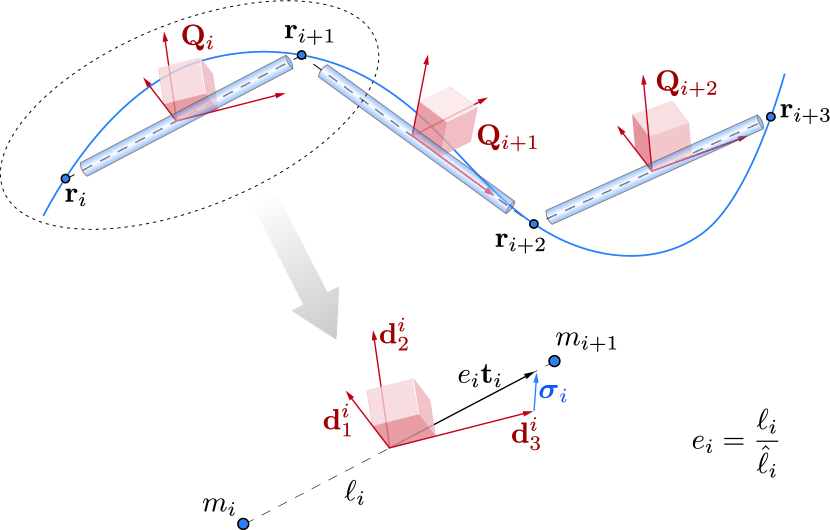
Figure 2: Discretization model. A discrete filament is represented through a set of vertices 𝐫(t)i=1,,N+1𝐫subscript𝑡𝑖1𝑁1\mathbf{r}(t)_{i=1,\dots,N+1} and a set of material frames Qi(t)={𝐝1i,𝐝2i,𝐝3i,}i=1,,NQ_{i}(t)=\{\mathbf{d}_{1}^{i},\mathbf{d}_{2}^{i},\mathbf{d}_{3}^{i},\}_{i=1,\dots,N}. Two consecutive vertices define an edge of length isubscript𝑖\ell_{i} along the tangent unit vector 𝐭isubscript𝐭𝑖\mathbf{t}_{i}. The dilatation is defined as ei=i/^isubscript𝑒𝑖subscript𝑖subscript^𝑖e_{i}=\ell_{i}/\hat{\ell}_{i}, where ^isubscript^𝑖\hat{\ell}_{i} is the edge rest length. The vector 𝝈i=ei𝐭i𝐝3isubscript𝝈𝑖subscript𝑒𝑖subscript𝐭𝑖superscriptsubscript𝐝3𝑖\boldsymbol{\sigma}_{i}=e_{i}\mathbf{t}_{i}-\mathbf{d}_{3}^{i} represents the discrete shear and axial strains. The mass mrsubscript𝑚𝑟m_{r} of the filament is discretized in pointwise concentrated masses mi=1,,n+1subscript𝑚𝑖1𝑛1m_{i=1,\dots,n+1} at the locations 𝐫isubscript𝐫𝑖\mathbf{r}_{i} for the purpose of advecting the vertices in time. For the evolution of 𝐐isubscript𝐐𝑖\mathbf{Q}_{i} in time, we consider instead the mass second moment of inertia 𝐉^i=1,,nsubscript^𝐉𝑖1𝑛\hat{\mathbf{J}}_{i=1,\dots,n} associated with the cylindrical elements depicted in blue.

III.1 Rotations

Bending and twisting deformations of a filament involve rotations of its material frame 𝐐𝐐\mathbf{Q} in space and time. To numerically simulate the rod, it is critical to represent and efficiently compute these nonlinear geometric transformations fast and accurately. A convenient way to express rotations in space or time is the matrix exponential Baillieul:1987 ; Levi:1996 ; Goriely:2000 . Assuming that the matrix 𝐑𝐑\mathbf{R} denotes the rotation by the angle θ𝜃\theta about the unit vector axis 𝐮𝐮\mathbf{u}, then this rotation can be expressed through the exponential matrix 𝐑=eθ𝐮:33×3:𝐑superscript𝑒𝜃𝐮superscript3superscript33\mathbf{R}=e^{\theta\mathbf{u}}:\mathbb{R}^{3}\rightarrow\mathbb{R}^{3\times 3}, and efficiently computed via the Rodrigues formula Rodrigues:1840

eθ𝐮=𝟏+sinθ𝐔+(1cosθ)𝐔𝐔.superscript𝑒𝜃𝐮1𝜃𝐔1𝜃𝐔𝐔e^{\theta\mathbf{u}}=\boldsymbol{1}+\sin\theta\mathbf{U}+(1-\cos\theta)\mathbf{U}\mathbf{U}. (16)

Here 𝐔3×3𝐔superscript33\mathbf{U}\in\mathbb{R}^{3\times 3} represents the skew-symmetric matrix associated with the unit vector 𝐮𝐮\mathbf{u}

𝐔=[𝐮]×=(0u3u2u30u1u2u10),𝐮=[𝐔]×1=(U3,2U3,1U2,1),formulae-sequence𝐔subscriptdelimited-[]𝐮0subscript𝑢3subscript𝑢2subscript𝑢30subscript𝑢1subscript𝑢2subscript𝑢10𝐮subscriptsuperscriptdelimited-[]𝐔1subscript𝑈32subscript𝑈31subscript𝑈21\mathbf{U}=[\mathbf{u}]_{\times}=\left(\begin{array}[]{ccc}0&-u_{3}&u_{2}\\ u_{3}&0&-u_{1}\\ -u_{2}&u_{1}&0\end{array}\right),~{}~{}~{}~{}~{}~{}~{}\mathbf{u}=[\mathbf{U}]^{-1}_{\times}=\left(\begin{array}[]{c}~{}~{}U_{3,2}\\ -U_{3,1}\\ ~{}~{}U_{2,1}\end{array}\right),

where the operator []×:33×3:subscriptdelimited-[]superscript3superscript33[\cdot]_{\times}:\mathbb{R}^{3}\rightarrow\mathbb{R}^{3\times 3} allows us to transform a vector into the corresponding skew-symmetric matrix, and vice versa []×1:3×33:subscriptsuperscriptdelimited-[]1superscript33superscript3[\cdot]^{-1}_{\times}:\mathbb{R}^{3\times 3}\rightarrow\mathbb{R}^{3}.

Conversely, given a rotation matrix 𝐑𝐑\mathbf{R}, the corresponding rotation vector can be directly computed via the matrix logarithm operator log():3×33:superscript33superscript3\log(\cdot):\mathbb{R}^{3\times 3}\rightarrow\mathbb{R}^{3}

θ𝐮=log(𝐑)={𝟎if θ=0θ2sinθ[𝐑𝐑T]×1if θ0,θ(π,π),θ=arccos(tr𝐑12).formulae-sequence𝜃𝐮𝐑cases0if 𝜃0𝜃2𝜃subscriptsuperscriptdelimited-[]𝐑superscript𝐑𝑇1formulae-sequenceif 𝜃0𝜃𝜋𝜋𝜃𝑡𝑟𝐑12\theta\mathbf{u}=\log\left(\mathbf{R}\right)=\begin{dcases}\mathbf{0}&\text{if }\theta=0\\ \frac{\theta}{2\sin\theta}\left[\mathbf{R}-\mathbf{R}^{T}\right]^{-1}_{\times}&\text{if }\theta\neq 0,\theta\in(-\pi,\pi)\end{dcases},~{}~{}~{}~{}~{}~{}~{}~{}\theta=\arccos\left(\frac{tr\mathbf{R}-1}{2}\right).

It is important to notice that the rotation axis 𝐮𝐮\mathbf{u} is expressed in the material frame of reference associated with the matrix 𝐑𝐑\mathbf{R} (or 𝐐𝐐\mathbf{Q}). With these tools in hand, we now proceed to outline our numerical scheme.

III.2 Spatial discretization

Drawing from previous studies of unshearable and inextensible rods Spillmann:2007 ; Bergou:2008 ; Sobottka:2008 , we capture the deformation of a filament in three-dimensional space via the time evolution of a discrete set of vertices 𝐫i(t)3,i[1,n+1]formulae-sequencesubscript𝐫𝑖𝑡superscript3𝑖1𝑛1\mathbf{r}_{i}(t)\in\mathbb{R}^{3},i\in[1,n+1] and a discrete set of material frames 𝐐i(t)3×3,i[1,n]formulae-sequencesubscript𝐐𝑖𝑡superscript33𝑖1𝑛\mathbf{Q}_{i}(t)\in\mathbb{R}^{3\times 3},i\in[1,n], as illustrated in Fig. 2.

Each vertex is associated with the following discrete quantities

𝐫i=1,,n+1subscript𝐫𝑖1𝑛1\displaystyle\mathbf{r}_{i=1,\dots,n+1} \displaystyle\rightarrow 𝐯i=𝐫it,mi,𝐅i,subscript𝐯𝑖subscript𝐫𝑖𝑡subscript𝑚𝑖subscript𝐅𝑖\displaystyle\mathbf{v}_{i}=\frac{\partial\mathbf{r}_{i}}{\partial t},~{}~{}~{}~{}m_{i},~{}~{}~{}~{}\mathbf{F}_{i}, (17)

where 𝐯isubscript𝐯𝑖\mathbf{v}_{i} is the velocity , misubscript𝑚𝑖m_{i} is a pointwise concentrated mass, and 𝐅isubscript𝐅𝑖\mathbf{F}_{i} is the external force given in Eq. (14).

Each material frame is associated with an edge isubscriptbold-ℓ𝑖\boldsymbol{\ell}_{i} connecting two consecutive vertices, and with the related discrete quantities

𝐐i=1,,nsubscript𝐐𝑖1𝑛\displaystyle\mathbf{Q}_{i=1,\dots,n} \displaystyle\rightarrow i=𝐫i+1𝐫i,i=|i|,^i=|^i|,ei=i^i,𝐭i=ii,formulae-sequencesubscriptbold-ℓ𝑖subscript𝐫𝑖1subscript𝐫𝑖formulae-sequencesubscript𝑖subscriptbold-ℓ𝑖formulae-sequencesubscript^𝑖subscript^bold-ℓ𝑖formulae-sequencesubscript𝑒𝑖subscript𝑖subscript^𝑖subscript𝐭𝑖subscriptbold-ℓ𝑖subscript𝑖\displaystyle\boldsymbol{\ell}_{i}=\mathbf{r}_{i+1}-\mathbf{r}_{i},~{}~{}~{}~{}\ell_{i}=|\boldsymbol{\ell}_{i}|,~{}~{}~{}~{}\hat{\ell}_{i}=|\hat{\boldsymbol{\ell}}_{i}|,~{}~{}~{}~{}e_{i}=\frac{\ell_{i}}{\hat{\ell}_{i}},~{}~{}~{}~{}{\mathbf{t}_{i}=\frac{\boldsymbol{\ell}_{i}}{\ell_{i}}}, (18)
𝝈i=𝐐i(ei𝐭i𝐝i3),𝝎i,A^i,𝐉^i,𝐁^i,𝐒^i,𝐂i,subscriptsuperscript𝝈𝑖subscript𝐐𝑖subscript𝑒𝑖subscript𝐭𝑖subscriptsuperscript𝐝3𝑖subscriptsuperscript𝝎𝑖subscript^𝐴𝑖subscript^𝐉𝑖subscript^𝐁𝑖subscript^𝐒𝑖subscriptsuperscript𝐂𝑖\displaystyle\boldsymbol{\sigma}^{i}_{\mathcal{L}}=\mathbf{Q}_{i}(e_{i}\mathbf{t}_{i}-\mathbf{d}^{3}_{i}),~{}~{}~{}~{}\boldsymbol{\omega}^{i}_{\mathcal{L}},~{}~{}~{}~{}\hat{A}_{i},~{}~{}~{}~{}\hat{\mathbf{J}}_{i},~{}~{}~{}~{}\hat{\mathbf{B}}_{i},~{}~{}~{}~{}\hat{\mathbf{S}}_{i},~{}~{}~{}~{}\mathbf{C}^{i}_{\mathcal{L}},

where i=|i|subscript𝑖subscriptbold-ℓ𝑖\ell_{i}=|\boldsymbol{\ell}_{i}|, ^i=|^i|subscript^𝑖subscript^bold-ℓ𝑖\hat{\ell}_{i}=|\hat{\boldsymbol{\ell}}_{i}|, ei=i/^isubscript𝑒𝑖subscript𝑖subscript^𝑖e_{i}=\ell_{i}/\hat{\ell}_{i} are the edge current length, reference length and dilatation factor, 𝐭isubscript𝐭𝑖\mathbf{t}_{i} is the discrete tangent vector, 𝝈isubscriptsuperscript𝝈𝑖\boldsymbol{\sigma}^{i}_{\mathcal{L}} is the discrete shear/axial strain vector, 𝝎isubscriptsuperscript𝝎𝑖\boldsymbol{\omega}^{i}_{\mathcal{L}} is the discrete angular velocity, A^isubscript^𝐴𝑖\hat{A}_{i}, 𝐉^isubscript^𝐉𝑖\hat{\mathbf{J}}_{i}, 𝐁^isubscript^𝐁𝑖\hat{\mathbf{B}}_{i}, 𝐒^isubscript^𝐒𝑖\hat{\mathbf{S}}_{i} are the edge reference cross section area, mass second moment of inertia, bend/twist matrix and shear/stretch matrix, and finally 𝐂isubscriptsuperscript𝐂𝑖\mathbf{C}^{i}_{\mathcal{L}} is the external couple given in Eq. (15).

Whereas in the continuum setting (Section II) all quantities are defined pointwise, in a discrete setting some quantities, and in particular 𝜿subscript𝜿\boldsymbol{\kappa}_{\mathcal{L}}, are naturally expressed in an integrated form over the domain 𝓓𝓓\boldsymbol{\mathcal{D}} along the filament Grinspun:2006 ; Bergou:2008 . Any integrated quantity divided by the corresponding integration domain length 𝒟=|𝓓|𝒟𝓓\mathcal{D}=|\boldsymbol{\mathcal{D}}| is equivalent to its pointwise average. In the context of our discretization the domain 𝓓𝓓\boldsymbol{\mathcal{D}} becomes the Voronoi region 𝓓isubscript𝓓𝑖\boldsymbol{\mathcal{D}}_{i} of length

𝒟i=i+1+i2,subscript𝒟𝑖subscript𝑖1subscript𝑖2\mathcal{D}_{i}=\frac{\ell_{i+1}+\ell_{i}}{2}, (19)

which is defined only for the interior vertices 𝐫i=1,,n1(int)subscriptsuperscript𝐫𝑖𝑛𝑡𝑖1𝑛1\mathbf{r}^{(int)}_{i=1,\dots,n-1}. Each interior vertex is then also associated with the following discrete quantities

𝐫i=1,,n1(int)subscriptsuperscript𝐫𝑖𝑛𝑡𝑖1𝑛1\displaystyle\mathbf{r}^{(int)}_{i=1,\dots,n-1} \displaystyle\rightarrow 𝒟i,𝒟^i,i=𝒟i𝒟^i,𝜿^i=log(𝐐i+1𝐐iT)𝒟^i,𝓑^i=𝐁^i+1^i+1+𝐁^i^i2𝒟^i,formulae-sequencesubscript𝒟𝑖subscript^𝒟𝑖subscript𝑖subscript𝒟𝑖subscript^𝒟𝑖formulae-sequencesubscriptsuperscript^𝜿𝑖subscript𝐐𝑖1subscriptsuperscript𝐐𝑇𝑖subscript^𝒟𝑖subscript^𝓑𝑖subscript^𝐁𝑖1subscript^𝑖1subscript^𝐁𝑖subscript^𝑖2subscript^𝒟𝑖\displaystyle\mathcal{D}_{i},~{}~{}~{}\hat{\mathcal{D}}_{i},~{}~{}~{}\mathcal{E}_{i}=\frac{\mathcal{D}_{i}}{\hat{\mathcal{D}}_{i}},~{}~{}~{}\hat{\boldsymbol{\kappa}}^{i}_{\mathcal{L}}=\frac{\log(\mathbf{Q}_{i+1}\mathbf{Q}^{T}_{i})}{\hat{\mathcal{D}}_{i}},~{}~{}~{}\hat{\boldsymbol{\mathcal{B}}}_{i}=\frac{\hat{\mathbf{B}}_{i+1}\hat{\ell}_{i+1}+\hat{\mathbf{B}}_{i}\hat{\ell}_{i}}{2\hat{\mathcal{D}}_{i}}, (20)

where 𝒟^isubscript^𝒟𝑖\hat{\mathcal{D}}_{i} is the Voronoi domain length at rest and isubscript𝑖\mathcal{E}_{i} is Voronoi region dilatation factor. Recalling that the generalized curvature expresses a rotation per unit length about its axis, then the quantity 𝒟^i𝜿^isubscript^𝒟𝑖subscriptsuperscript^𝜿𝑖\hat{\mathcal{D}}_{i}\hat{\boldsymbol{\kappa}}^{i}_{\mathcal{L}} naturally expresses the rotation that transforms a material frame 𝐐isubscript𝐐𝑖\mathbf{Q}_{i} to its neighbour 𝐐i+1subscript𝐐𝑖1\mathbf{Q}_{i+1} over the segment size 𝒟^isubscript^𝒟𝑖\hat{\mathcal{D}}_{i} along the rod. Therefore, the relation e𝒟^i𝜿^i𝐐i=𝐐i+1superscript𝑒subscript^𝒟𝑖subscriptsuperscript^𝜿𝑖subscript𝐐𝑖subscript𝐐𝑖1e^{\hat{\mathcal{D}}_{i}\hat{\boldsymbol{\kappa}}^{i}_{\mathcal{L}}}\mathbf{Q}_{i}=\mathbf{Q}_{i+1} holds, so that 𝜿^i=log(𝐐i+1𝐐iT)/𝒟^isubscriptsuperscript^𝜿𝑖subscript𝐐𝑖1subscriptsuperscript𝐐𝑇𝑖subscript^𝒟𝑖\hat{\boldsymbol{\kappa}}^{i}_{\mathcal{L}}=\log(\mathbf{Q}_{i+1}\mathbf{Q}^{T}_{i})/\hat{\mathcal{D}}_{i}. Finally, we introduce the bend/twist stiffness matrix 𝓑^isubscript^𝓑𝑖\hat{\boldsymbol{\mathcal{B}}}_{i} consistent with the Voronoi representation.

Then, we may discretize the governing Eqs. (12-15) so that they read

𝐫itsubscript𝐫𝑖𝑡\displaystyle\frac{\partial\mathbf{r}_{i}}{\partial t} =\displaystyle= 𝐯i,i=[1,n+1]subscript𝐯𝑖𝑖1𝑛1\displaystyle\mathbf{v}_{i},\hskip 213.39566pti=[1,n+1] (21)
𝐝i,jtsubscript𝐝𝑖𝑗𝑡\displaystyle\frac{\partial\mathbf{d}_{i,j}}{\partial t} =\displaystyle= (𝐐iT𝝎i)×𝐝i,j,i=[1,n],j=1,2,3formulae-sequencesuperscriptsubscript𝐐𝑖𝑇subscriptsuperscript𝝎𝑖subscript𝐝𝑖𝑗𝑖1𝑛𝑗123\displaystyle(\mathbf{Q}_{i}^{T}\boldsymbol{\omega}^{i}_{\mathcal{L}})\times\mathbf{d}_{i,j},\hskip 128.0374pti=[1,n],~{}j=1,2,3 (22)
mi𝐯itsubscript𝑚𝑖subscript𝐯𝑖𝑡\displaystyle m_{i}\cdot\frac{\partial\mathbf{v}_{i}}{\partial t} =\displaystyle= Δh(𝐐iT𝐒^i𝝈iei)+𝐅i,i=[1,n+1]superscriptΔsuperscriptsubscript𝐐𝑖𝑇subscript^𝐒𝑖subscriptsuperscript𝝈𝑖subscript𝑒𝑖subscript𝐅𝑖𝑖1𝑛1\displaystyle\Delta^{h}\left(\frac{\mathbf{Q}_{i}^{T}\hat{\mathbf{S}}_{i}\boldsymbol{\sigma}^{i}_{\mathcal{L}}}{e_{i}}\right)+\mathbf{F}_{i},\hskip 128.0374pti=[1,n+1] (23)
𝐉^iei𝝎itsubscript^𝐉𝑖subscript𝑒𝑖subscriptsuperscript𝝎𝑖𝑡\displaystyle\frac{\hat{\mathbf{J}}_{i}}{e_{i}}\cdot\frac{\partial\boldsymbol{\omega}^{i}_{\mathcal{L}}}{\partial t} =\displaystyle= Δh(𝓑^i𝜿^ii3)+𝒜h(𝜿^i×𝓑^i𝜿^ii3𝒟^i)+(𝐐i𝐭i×𝐒^i𝝈i)^isuperscriptΔsubscript^𝓑𝑖superscriptsubscript^𝜿𝑖superscriptsubscript𝑖3superscript𝒜superscriptsubscript^𝜿𝑖subscript^𝓑𝑖superscriptsubscript^𝜿𝑖superscriptsubscript𝑖3subscript^𝒟𝑖subscript𝐐𝑖subscript𝐭𝑖subscript^𝐒𝑖subscriptsuperscript𝝈𝑖subscript^𝑖\displaystyle\Delta^{h}\left(\frac{\hat{\boldsymbol{\mathcal{B}}}_{i}\hat{\boldsymbol{\kappa}}_{\mathcal{L}}^{i}}{\mathcal{E}_{i}^{3}}\right)+\mathcal{A}^{h}\left(\frac{\hat{\boldsymbol{\kappa}}_{\mathcal{L}}^{i}\times\hat{\boldsymbol{\mathcal{B}}}_{i}\hat{\boldsymbol{\kappa}}_{\mathcal{L}}^{i}}{\mathcal{E}_{i}^{3}}\hat{\mathcal{D}}_{i}\right)+\left(\mathbf{Q}_{i}\mathbf{t}_{i}\times\hat{\mathbf{S}}_{i}\boldsymbol{\sigma}^{i}_{\mathcal{L}}\right)\hat{\ell}_{i} (24)
+(𝐉^i𝝎iei)×𝝎i+𝐉^i𝝎iei2eit+𝐂i,i=[1,n]subscript^𝐉𝑖subscriptsuperscript𝝎𝑖subscript𝑒𝑖subscriptsuperscript𝝎𝑖subscript^𝐉𝑖subscriptsuperscript𝝎𝑖superscriptsubscript𝑒𝑖2subscript𝑒𝑖𝑡subscriptsuperscript𝐂𝑖𝑖1𝑛\displaystyle+\left(\hat{\mathbf{J}}_{i}\cdot\frac{\boldsymbol{\omega}^{i}_{\mathcal{L}}}{e_{i}}\right)\times\boldsymbol{\omega}^{i}_{\mathcal{L}}+\frac{\hat{\mathbf{J}}_{i}\boldsymbol{\omega}^{i}_{\mathcal{L}}}{e_{i}^{2}}\cdot\frac{\partial e_{i}}{\partial t}+\mathbf{C}^{i}_{\mathcal{L}},\hskip 71.13188pti=[1,n]

where Δh:{3}N{3}N+1:superscriptΔsubscriptsuperscript3𝑁subscriptsuperscript3𝑁1\Delta^{h}:\{\mathbb{R}^{3}\}_{N}\rightarrow\{\mathbb{R}^{3}\}_{N+1} is the discrete difference operator and 𝒜h:{3}N{3}N+1:superscript𝒜subscriptsuperscript3𝑁subscriptsuperscript3𝑁1\mathcal{A}^{h}:\{\mathbb{R}^{3}\}_{N}\rightarrow\{\mathbb{R}^{3}\}_{N+1} is the averaging operator to transform integrated quantities over the domain 𝒟𝒟\mathcal{D} to their point-wise counterparts. We note that ΔhsuperscriptΔ\Delta^{h} and 𝒜hsuperscript𝒜\mathcal{A}^{h} operate on a set of N𝑁N vectors and returns N+1𝑁1N+1 vectors, consistent with Eqs. (21-24) (see the Appendix for further details).

III.3 Time discretization

While the above equations are conservative and preserve energy, in general when additional physical effects and interactions with complex environments are considered, the equations of motion are not conservative. We choose a symplectic, second-order Verlet scheme to integrate the equations of motion in time so that our numerical scheme is energy-preserving in the case of conservative dynamics. We note that despite the failure of Verlet schemes to integrate rotational equations of motion when represented by quaternions, in our case their use is acceptable as rotations are represented instead by Euler angles Kol:1997 .

The second order position Verlet time integrator is structured in three blocks: a first half-step updates the linear and angular positions, followed by the evaluation of local linear and angular accelerations, and finally a second half-step updates the linear and angular positions again. Therefore, it entails only one right hand side evaluation of Eqs. (23, 24), the most computationally expensive operation (see Appendix for details).

This algorithm strikes a balance between computing costs, numerical accuracy and implementation modularity: by foregoing an implicit integration scheme we can incorporate a number of additional physical effects and soft constraints, even though this may come at the expense of computational efficiency.

III.4 Validation

We first validate our proposed methodology against a number of benchmark problems with analytic solutions and examine the convergence properties of our approach. Three case studies serve to characterize the competition between bending and twisting effects in the context of helical buckling, dynamic stretching of a loaded rod under gravity, and the competition between shearing and bending in the context of a Timoshenko beam. Further validations reported in the Appendix include Euler and Mitchell buckling due to compression or twist, and stretching and twisting vibrations.

III.4.1 Helical buckling instability

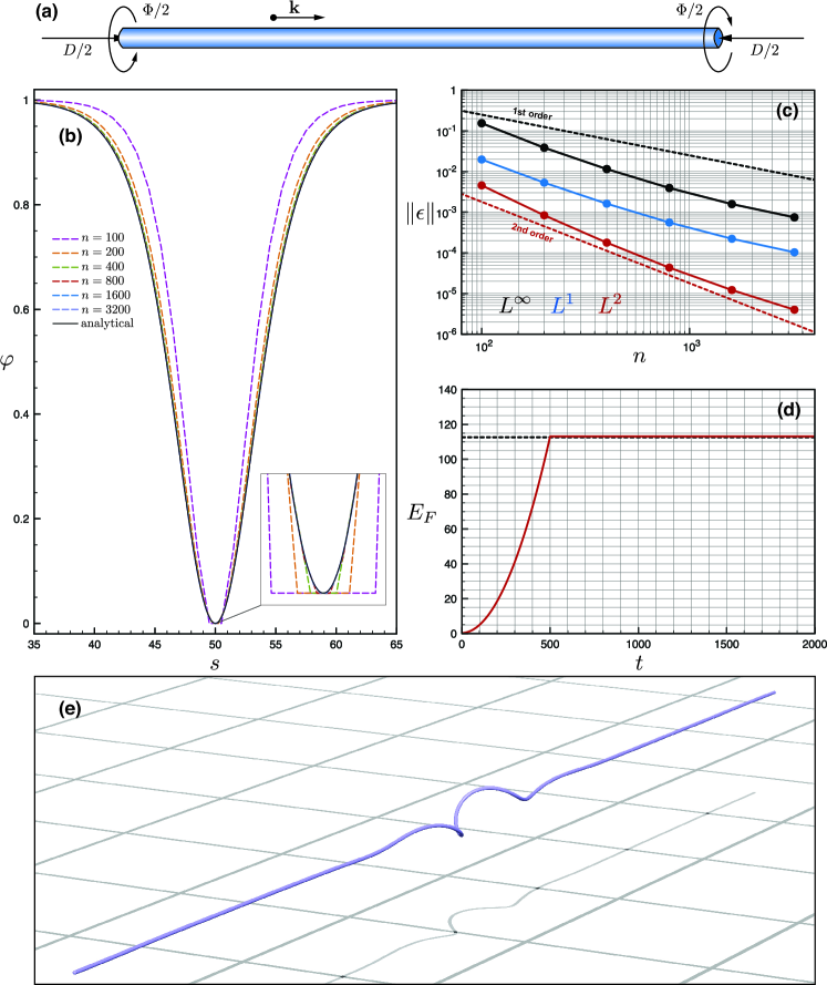
We validate our discrete derivative operators beyond the onset of instability (see Euler and Mitchell buckling tests in the Appendix) for a long straight, isotropic, inextensible, and unshearable rod undergoing bending and twisting. The filament is characterized by the length L𝐿L and by the bending and twist stiffnesses α𝛼\alpha and β𝛽\beta. The clamped ends of the rod are pulled together in the axial direction 𝐤𝐤\mathbf{k} with a slack D/2𝐷2D/2 and simultaneously twisted by the angle Φ/2Φ2\Phi/2, as illustrated in Fig. 3a. Under these conditions the filament buckles into a localized helical shape (Fig. 3e).

The nonlinear equilibrium configuration 𝐫eqsubscript𝐫𝑒𝑞\mathbf{r}_{eq} of the rod can be analitycally determined Coyne:1990 ; vanDerHeijden:2000 ; Neukirch:2002 ; vanDerHeijden:2003 in terms of the total applied slack D𝐷D and twist ΦΦ\Phi. We denote the magnitude of the twisting torque and tension acting on both ends and projected on 𝐤𝐤\mathbf{k} by Mhsubscript𝑀M_{h} and Thsubscript𝑇T_{h}, respectively. Their normalized counterparts mh=MhL/(2πα)subscript𝑚subscript𝑀𝐿2𝜋𝛼m_{h}=M_{h}L/(2\pi\alpha) and th=ThL2/(4π2α)subscript𝑡subscript𝑇superscript𝐿24superscript𝜋2𝛼t_{h}=T_{h}L^{2}/(4\pi^{2}\alpha) can be computed via the ‘semi-finite’ correction approach Neukirch:2002 by solving the system

{DL=4π2th(1mh24th),Φ=2πmhβ/α+4arccos(mh2th).cases𝐷𝐿4superscript𝜋2subscript𝑡1superscriptsubscript𝑚24subscript𝑡otherwiseΦ2𝜋subscript𝑚𝛽𝛼4subscript𝑚2subscript𝑡otherwise\begin{dcases}\frac{D}{L}=\sqrt{\frac{4}{\pi^{2}t_{h}}\left(1-\frac{m_{h}^{2}}{4t_{h}}\right)},\\ \Phi=\frac{2\pi m_{h}}{\beta/\alpha}+4\arccos\left(\frac{m_{h}}{2\sqrt{t_{h}}}\right).\end{dcases}

Then, the analytical form of 𝐫eqsubscript𝐫𝑒𝑞\mathbf{r}_{eq} can be expressed vanDerHeijden:2003 as

𝐫eqsubscript𝐫𝑒𝑞\displaystyle\mathbf{r}_{eq} =\displaystyle= L[12πth4thmh2 sech(πs¯4thmh2)sin(mhπs¯)]𝐢𝐿delimited-[]12𝜋subscript𝑡4subscript𝑡subscriptsuperscript𝑚2 sech𝜋¯𝑠4subscript𝑡subscriptsuperscript𝑚2subscript𝑚𝜋¯𝑠𝐢\displaystyle L\left[\frac{1}{2\pi t_{h}}\sqrt{4t_{h}-m^{2}_{h}}\text{ sech}\left(\pi\bar{s}\sqrt{4t_{h}-m^{2}_{h}}\right)\sin(m_{h}\pi\bar{s})\right]\mathbf{i}
L[12πth4thmh2 sech(πs¯4thmh2)cos(mhπs¯)]𝐣𝐿delimited-[]12𝜋subscript𝑡4subscript𝑡subscriptsuperscript𝑚2 sech𝜋¯𝑠4subscript𝑡subscriptsuperscript𝑚2subscript𝑚𝜋¯𝑠𝐣\displaystyle-L\left[\frac{1}{2\pi t_{h}}\sqrt{4t_{h}-m^{2}_{h}}\text{ sech}\left(\pi\bar{s}\sqrt{4t_{h}-m^{2}_{h}}\right)\cos(m_{h}\pi\bar{s})\right]\mathbf{j}
+L[s¯12πth4thmh2 tanh(πs¯4thmh2)]𝐤,𝐿delimited-[]¯𝑠12𝜋subscript𝑡4subscript𝑡subscriptsuperscript𝑚2 tanh𝜋¯𝑠4subscript𝑡subscriptsuperscript𝑚2𝐤\displaystyle+L\left[\bar{s}-\frac{1}{2\pi t_{h}}\sqrt{4t_{h}-m^{2}_{h}}\text{ tanh}\left(\pi\bar{s}\sqrt{4t_{h}-m^{2}_{h}}\right)\right]\mathbf{k},

where s¯=s/L0.5¯𝑠𝑠𝐿0.5\bar{s}=s/L-0.5 is the normalized arc-length 0.5s¯0.50.5¯𝑠0.5-0.5\leq\bar{s}\leq 0.5. Here we make use of Eq. (III.4.1) to investigate the convergence properties of our solver in the limit of refinement. To compare analytical and numerical solutions, a metric invariant to rotations about 𝐤𝐤\mathbf{k} is necessary. Following Bergou et al.Bergou:2008 , we rely on the definition of the envelope φ𝜑\varphi

φ=cosθcosθmax1cosθmax,θ=arccos(𝐭𝐤)formulae-sequence𝜑𝜃subscript𝜃𝑚𝑎𝑥1subscript𝜃𝑚𝑎𝑥𝜃𝐭𝐤\varphi=\frac{\cos\theta-\cos\theta_{max}}{1-\cos\theta_{max}},~{}~{}~{}~{}~{}~{}\theta=\arccos(\mathbf{t}\cdot\mathbf{k})\\ (26)

where θ𝜃\theta is the angular deviation of the tangent 𝐭𝐭\mathbf{t} from the axial direction 𝐤𝐤\mathbf{k}, and θmaxsubscript𝜃𝑚𝑎𝑥\theta_{max} is the corresponding maximum value along the filament. The envelope φ𝜑\varphi relative to the analytical solution of Eq. (III.4.1), and φnsuperscript𝜑𝑛\varphi^{n} relative to a numerical model of n𝑛n discretization elements can be estimated via finite differences. This allows us to determine the convergence order of the solver by means of the norms L1(ϵ)superscript𝐿1italic-ϵL^{1}(\epsilon), L2(ϵ)superscript𝐿2italic-ϵL^{2}(\epsilon) and L(ϵ)superscript𝐿italic-ϵL^{\infty}(\epsilon) of the error ϵ=φφnitalic-ϵnorm𝜑superscript𝜑𝑛\epsilon=\|\varphi-\varphi^{n}\|.

We simulate the problem illustrated in Fig. 3 at different space-time resolutions. The straight rod originally at rest is twisted and compressed at a constant rate during the period Ttwistsubscript𝑇twistT_{\text{twist}}. Subsequently, the ends of the rod are held in their final configurations for the period Trelaxsubscript𝑇relaxT_{\text{relax}} to allow the internal energy to dissipate (according to the model of Section IV.0.1) until the steady state is reached. Simulations are carried out progressively refining the spatial discretization δl=L/n𝛿𝑙𝐿𝑛\delta l=L/n by varying n=1003200𝑛1003200n=100-3200 and the time discretization δt𝛿𝑡\delta t is kept proportional to δl𝛿𝑙\delta l, as reported in Fig. 3.

As can be seen in Fig. (3)b,c,e the numerical solutions converge to the analytical one with second order in time and space, consistent with our spatial and temporal discretization schemes. Moreover, to further validate the energy conserving properties of the solver, we turn off the internal dissipation (Fig. 3d) and observe that the total energy of the filament EFsubscript𝐸𝐹E_{F} is constant after Ttwistsubscript𝑇twistT_{\text{twist}} and matches its theoretical value EF=(MhΦ+ThD)/2subscript𝐸𝐹subscript𝑀Φsubscript𝑇𝐷2E_{F}=(M_{h}\Phi+T_{h}D)/2.

Refer to caption
Figure 3: Time-space convergence study for localized helical buckling. (a) We consider a rod originally straight whose ends are pulled together in the axial direction 𝐤𝐤\mathbf{k} with a slack D/2𝐷2D/2 and simultaneously twisted by the angle Φ/2Φ2\Phi/2. (b) Comparison between the analytical envelope function φ(s)𝜑𝑠\varphi(s) and numerical approximations φn(s)superscript𝜑𝑛𝑠\varphi^{n}(s) at different levels of time-space resolution. Here, the time discretization δt𝛿𝑡\delta t is slaved by the spatial discretization δl=L/n𝛿𝑙𝐿𝑛\delta l=L/n according to δt=103δl𝛿𝑡superscript103𝛿𝑙\delta t=10^{-3}\delta l s. (c) Norms L(ϵ)superscript𝐿italic-ϵL^{\infty}(\epsilon) (black), L1(ϵ)superscript𝐿1italic-ϵL^{1}(\epsilon) (blue) and L2(ϵ)superscript𝐿2italic-ϵL^{2}(\epsilon) (red) are plotted against the number of discretization elements n𝑛n. (d) Time evolution of the total energy of a rod (n=800𝑛800n=800, here the energy is computed assuming quadratic functionals, a suitable representation for an inextensible rod) simulated assuming no dissipation γ=0𝛾0\gamma=0 (red line) versus the theoretical total energy EF=(MhΦ+ThD)/2subscript𝐸𝐹subscript𝑀Φsubscript𝑇𝐷2E_{F}=(M_{h}\Phi+T_{h}D)/2 (black dashed line). (e) Equilibrium rod configuration 𝐫eqnsubscriptsuperscript𝐫𝑛𝑒𝑞\mathbf{r}^{n}_{eq} numerically obtained given the discretization n=800𝑛800n=800, and assuming dissipation. For all studies, unless specified otherwise, we used the following settings: length L=100𝐿100L=100 m, twist Φ=272πΦ272𝜋\Phi=27\cdot 2\pi, slack D=3𝐷3D=3 m, linear mass density ρ=1𝜌1\rho=1 kg/m, bending stiffness α=1.345𝛼1.345\alpha=1.345 Nm2, twisting stiffness β=0.789𝛽0.789\beta=0.789 Nm2, shear/stretch matrix 𝐒=105𝟏𝐒superscript1051\mathbf{S}=10^{5}\cdot\boldsymbol{1} N, bend/twist matrix 𝐁=diag(α,α,β)𝐁diag𝛼𝛼𝛽\mathbf{B}=\text{diag}(\alpha,\alpha,\beta) Nm2, dissipation constant γ=102𝛾superscript102\gamma=10^{-2} kg/(ms), radius r=0.35𝑟0.35r=0.35 m, twisting time Ttwist=500subscript𝑇twist500T_{\text{twist}}=500 s, relaxation time Trelax=104subscript𝑇relaxsuperscript104T_{\text{relax}}=10^{4} s.

III.4.2 Vertical oscillations under gravity

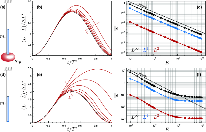
We consider a system in which a rod hanging from one end and subject to gravity g𝑔g oscillates due to a mass mpsubscript𝑚𝑝m_{p} suspended at the other end, and due to its own mass mrsubscript𝑚𝑟m_{r}, as depicted in Fig. 4a,d. This system is analogous to a mass-spring oscillator. The static solution is then obtained by integrating the infinitesimal elongations along the spring due to the local load Galloni:1979 , yielding the total equilibrium extension

ΔL=gmeqk=g(mp+mr/ξ)k,Δsuperscript𝐿𝑔subscript𝑚𝑒𝑞𝑘𝑔subscript𝑚𝑝subscript𝑚𝑟𝜉𝑘\Delta L^{*}=\frac{gm_{eq}}{k}=\frac{g(m_{p}+m_{r}/\xi)}{k}, (27)

where k𝑘k is the spring constant, ξ=2𝜉2\xi=2 is a constant factor, and meq=mp+mr/ξsubscript𝑚𝑒𝑞subscript𝑚𝑝subscript𝑚𝑟𝜉m_{eq}=m_{p}+m_{r}/\xi is the equivalent mass. Thus, the final equilibrium length of the rod reads L=L^+ΔL𝐿^𝐿Δsuperscript𝐿L=\hat{L}+\Delta L^{*}, with L^^𝐿\hat{L} being the rest unstretched length.

The dynamic solution is instead characterized by oscillations of period Tsuperscript𝑇T^{*} and by the time varying length L(t)𝐿𝑡L(t) of the spring

T=2π(mp+mr/ξ)/k,L=L^+[1+sin(2πt/Tπ/2)]ΔL.formulae-sequencesuperscript𝑇2𝜋subscript𝑚𝑝subscript𝑚𝑟𝜉𝑘𝐿^𝐿delimited-[]12𝜋𝑡superscript𝑇𝜋2Δsuperscript𝐿T^{*}=2\pi\sqrt{(m_{p}+m_{r}/\xi)/k},~{}~{}~{}~{}~{}L=\hat{L}+[1+\sin(2\pi t/T^{*}-\pi/2)]\Delta L^{*}. (28)

In this case, unlike the static solution, the factor ξ𝜉\xi depends on the ratio mr/mpsubscript𝑚𝑟subscript𝑚𝑝m_{r}/m_{p}. In fact it can be shown Galloni:1979 that ξ3similar-to-or-equals𝜉3\xi\simeq 3 for mr/mp0subscript𝑚𝑟subscript𝑚𝑝0m_{r}/m_{p}\rightarrow 0, and ξπ2/4similar-to-or-equals𝜉superscript𝜋24\xi\simeq\pi^{2}/4 for mr/mpsubscript𝑚𝑟subscript𝑚𝑝m_{r}/m_{p}\rightarrow\infty.

The analytical results rely on the assumption of k𝑘k being constant in space and time, given a fixed ratio mr/mpsubscript𝑚𝑟subscript𝑚𝑝m_{r}/m_{p}. However, this condition is not met here since k(s,t)=EA(s,t)𝑘𝑠𝑡𝐸𝐴𝑠𝑡k(s,t)=EA(s,t) is a function of space and time, due to dilatation and mass conservation. Nevertheless, as the Young’s modulus E𝐸E\rightarrow\infty, that is as a soft filament becomes stiff, the constant kEA^𝑘𝐸^𝐴k\rightarrow E\hat{A} and our rod model must recover the behavior of the mass-spring oscillator. Indeed, Fig. 4b,c,e,f shows how the proposed numerical method converges to the analytical oscillation period Tsuperscript𝑇T^{*} and normalized longitudinal displacement (LL^)/ΔL𝐿^𝐿Δsuperscript𝐿(L-\hat{L})/\Delta L^{*} as E𝐸E increases.

Refer to caption
Figure 4: Vertical oscillation under gravity. (a,d) We consider a vertical rod of mass mrsubscript𝑚𝑟m_{r} clamped at the top and with a mass mpsubscript𝑚𝑝m_{p} attached to the free end. Assuming that the rod is stiff enough (i.e. kA^E=constsimilar-to-or-equals𝑘^𝐴𝐸constk\simeq\hat{A}E=\text{const}), it oscillates due to gravity around the equilibrium position L^+ΔL^𝐿Δsuperscript𝐿\hat{L}+\Delta L^{*}, where ΔL=g(mp+mr/2)/kΔsuperscript𝐿𝑔subscript𝑚𝑝subscript𝑚𝑟2𝑘\Delta L^{*}=g(m_{p}+m_{r}/2)/k with a period T=2π(mp+mr/ξ)/ksuperscript𝑇2𝜋subscript𝑚𝑝subscript𝑚𝑟𝜉𝑘T^{*}=2\pi\sqrt{(m_{p}+m_{r}/\xi)/k} with ξ3similar-to-or-equals𝜉3\xi\simeq 3 for mpmrmuch-greater-thansubscript𝑚𝑝subscript𝑚𝑟m_{p}\gg m_{r}, and ξπ2/4similar-to-or-equals𝜉superscript𝜋24\xi\simeq\pi^{2}/4 for mpmrmuch-less-thansubscript𝑚𝑝subscript𝑚𝑟m_{p}\ll m_{r}. Therefore, the rod oscillates according to L(t)=L^+[1+sin(2πt/Tπ/2)]ΔL𝐿𝑡^𝐿delimited-[]12𝜋𝑡superscript𝑇𝜋2Δsuperscript𝐿L(t)=\hat{L}+[1+\sin(2\pi t/T^{*}-\pi/2)]\Delta L^{*}. (a-b) Case mpmrmuch-greater-thansubscript𝑚𝑝subscript𝑚𝑟m_{p}\gg m_{r} with mp=100subscript𝑚𝑝100m_{p}=100 kg and mr=1subscript𝑚𝑟1m_{r}=1 kg. (b) By increasing the stiffness E=107𝐸superscript107E=10^{7}, 2\cdot107superscript10710^{7}, 3\cdot107superscript10710^{7}, 5\cdot107superscript10710^{7}, 108superscript10810^{8}, 1010superscript101010^{10} Pa, the simulated oscillations (red lines) approach the analytical solution (dashed black line). (c) Convergence to the analytical solution in the norms L(ϵ)superscript𝐿italic-ϵL^{\infty}(\epsilon) (black), L1(ϵ)superscript𝐿1italic-ϵL^{1}(\epsilon) (blue) and L2(ϵ)superscript𝐿2italic-ϵL^{2}(\epsilon) (red) with ϵ=L(t)LE(t)italic-ϵnorm𝐿𝑡superscript𝐿𝐸𝑡\epsilon=\|L(t)-L^{E}(t)\|, where LEsuperscript𝐿𝐸L^{E} is the length numerically obtained as a function of E𝐸E. (c-d) Case mpmrmuch-less-thansubscript𝑚𝑝subscript𝑚𝑟m_{p}\ll m_{r} with mp=0subscript𝑚𝑝0m_{p}=0 kg and mr=1subscript𝑚𝑟1m_{r}=1 kg. (e) By increasing the stiffness E=104𝐸superscript104E=10^{4}, 2\cdot104superscript10410^{4}, 3\cdot104superscript10410^{4}, 5\cdot104superscript10410^{4}, 105superscript10510^{5}, 2\cdot105superscript10510^{5}, 109superscript10910^{9} Pa, the simulated oscillations approach the analytical solution. (f) Convergence to the analytical solution in the norms L(ϵ)superscript𝐿italic-ϵL^{\infty}(\epsilon), L1(ϵ)superscript𝐿1italic-ϵL^{1}(\epsilon) and L2(ϵ)superscript𝐿2italic-ϵL^{2}(\epsilon) as a function of E𝐸E. For all studies, we used the following settings: gravity g=9.81𝑔9.81g=9.81 m/s2, rod density ρ=103𝜌superscript103\rho=10^{3} kg/m3, shear modulus G=2E/3𝐺2𝐸3G=2E/3 Pa, shear/stretch matrix 𝐒^=diag(4GA^/3,4GA^/3,EA^)^𝐒diag4𝐺^𝐴34𝐺^𝐴3𝐸^𝐴\hat{\mathbf{S}}=\text{diag}(4G\hat{A}/3,4G\hat{A}/3,E\hat{A}) N, bend/twist matrix 𝐁^=diag(EI^1,EI^2,GI^3)^𝐁diag𝐸subscript^𝐼1𝐸subscript^𝐼2𝐺subscript^𝐼3\hat{\mathbf{B}}=\text{diag}(E\hat{I}_{1},E\hat{I}_{2},G\hat{I}_{3}) Nm2, rest length L^=1^𝐿1\hat{L}=1 m, rest cross sectional area A^=mr/(L^ρ)^𝐴subscript𝑚𝑟^𝐿𝜌\hat{A}=~{}m_{r}/(\hat{L}\rho) m2, number of discretization elements n=100𝑛100n=100, timestep δt=T/106𝛿𝑡superscript𝑇superscript106\delta t=T^{*}/10^{6}, dissipation constant γ=0𝛾0\gamma=0.

III.4.3 Cantilever beam

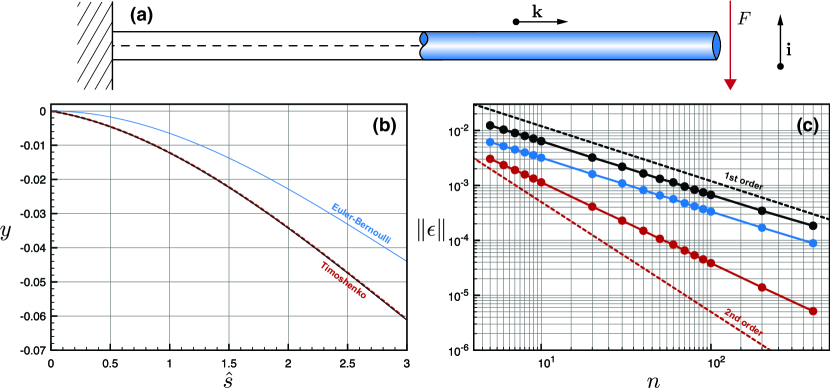
We consider now the effect of bend and shear simultaneously by validating our numerical methods against the Timoshenko cantilever of Fig. 5a. Timoshenko’s model accounts for bending elasticity, rotary inertia and shear deformations, building on classical beam theories by Rayleigh (bending elasticity and rotary inertia) and Euler-Bernoulli (bending elasticity only). The model captures the behavior of short or composite beams in which shear deformations effectively lower the stiffness of the rod Rao:1995 ; Gere:2001 .

We consider a beam clamped at one end s^=0^𝑠0\hat{s}=0 and subject to the downward force F𝐹F at the free end s^=L^^𝑠^𝐿\hat{s}=\hat{L}, as illustrated in Fig. 5a. The static solution for the displacement y𝑦y along the vertical direction 𝐢𝐢\mathbf{i} of the rod can then be analytically expressed as

y=FαcA^Gs^FL^2EI^1s^2+F6EI^1s^3,𝑦𝐹subscript𝛼𝑐^𝐴𝐺^𝑠𝐹^𝐿2𝐸subscript^𝐼1superscript^𝑠2𝐹6𝐸subscript^𝐼1superscript^𝑠3y=-\frac{F}{\alpha_{c}\hat{A}G}\hat{s}-\frac{F\hat{L}}{2E\hat{I}_{1}}\hat{s}^{2}+\frac{F}{6E\hat{I}_{1}}\hat{s}^{3}, (29)

where L^^𝐿\hat{L} is the length of the rod, A^^𝐴\hat{A} is the constant cross sectional area, I^1subscript^𝐼1\hat{I}_{1} is the area second moment of inertia about the axis 𝐣=𝐤×𝐢𝐣𝐤𝐢\mathbf{j}=\mathbf{k}\times\mathbf{i}, E𝐸E and G𝐺G are the Young’s and shear moduli, and αc=4/3subscript𝛼𝑐43\alpha_{c}=4/3 is the Timoshenko shear factor for circular sections and accounts for the fact that the shear stress varies over the section Gere:2001 . Furthermore, the Timoshenko (as well as Rayleigh and Euler-Bernoulli) theory relies on the assumption of small deflections, so that the horizontal coordinate x𝑥x along the direction 𝐤𝐤\mathbf{k} can be approximated by the arc-length s^^𝑠\hat{s} (Fig. 5a and Appendix for further details and derivation), hence the use of s^^𝑠\hat{s} in the above equation .

If the shear modulus G𝐺G approaches infinity or if the ratio EI^1/(αcL^2A^G)1much-greater-than𝐸subscript^𝐼1subscript𝛼𝑐superscript^𝐿2^𝐴𝐺1E\hat{I}_{1}/(\alpha_{c}\hat{L}^{2}\hat{A}G)\gg 1, then the Timoshenko model in the static case reduces to the Euler-Bernoulli approximation, yielding

y=FL^2EI^1s^2+F6EI^1s^3,𝑦𝐹^𝐿2𝐸subscript^𝐼1superscript^𝑠2𝐹6𝐸subscript^𝐼1superscript^𝑠3y=-\frac{F\hat{L}}{2E\hat{I}_{1}}\hat{s}^{2}+\frac{F}{6E\hat{I}_{1}}\hat{s}^{3}, (30)

as the shear term of Eq. (29) becomes negligible.

We compare our numerical model with these results by carrying out simulations of the cantilever beam of Fig. 5a in the time-space limit of refinement. As can be noticed in Fig. 5b the discrete solution recovers the Timoshenko one. Therefore, the solver correctly captures the role of shear that reduces the effective stiffness relative to the Euler-Bernoulli solution. Moreover, our approach is shown to converge to the analytical solution in all the norms L(ϵ)superscript𝐿italic-ϵL^{\infty}(\epsilon), L1(ϵ)superscript𝐿1italic-ϵL^{1}(\epsilon), L2(ϵ)superscript𝐿2italic-ϵL^{2}(\epsilon) of the error ϵ=yynitalic-ϵnorm𝑦superscript𝑦𝑛\epsilon=\|y-y^{n}\|, where ynsuperscript𝑦𝑛y^{n} is the vertical displacement numerically obtained in the refinement limit.

We note that the norms L(ϵ)superscript𝐿italic-ϵL^{\infty}(\epsilon) and L1(ϵ)superscript𝐿1italic-ϵL^{1}(\epsilon) exhibit first order convergence, while L2(ϵ)superscript𝐿2italic-ϵL^{2}(\epsilon) decays with a slope between first and second order. We attribute these results to the fact that while the Timoshenko solution does not consider axial extension or tension, it does rely on the assumption of small deflections (s^=x^𝑠𝑥\hat{s}=x), therefore effectively producing a dilatation of the rod. On the contrary, our solver does not assume small deflections and does not neglect axial extension, since the third entry of the matrix 𝐁𝐁\mathbf{B} has the finite value EA^𝐸^𝐴E\hat{A} (see Fig. 5 for details). This discrepancy is here empirically observed to decrease the convergence order.

These studies, together with the ones reported in the Appendix, complete the validation of the proposed numerical scheme and demonstrate the accuracy of our methodology in simulating soft filaments in simple settings.
Refer to caption
Figure 5: Time-space convergence study for a cantilever beam. (a) We consider the static solution of a beam clamped at one end s^=0^𝑠0\hat{s}=0 and subject to the downward force F𝐹F at the free end s^=L^^𝑠^𝐿\hat{s}=\hat{L}. (b) Comparison between the Timoshenko analytical y𝑦y (black lines) and numerical ynsuperscript𝑦𝑛y^{n} (with n=400𝑛400n=400, red dashed lines) vertical displacements with respect to the initial rod configuration. As a reference we report in blue the corresponding Euler-Bernoulli solution. (c) Norms L(ϵ)superscript𝐿italic-ϵL^{\infty}(\epsilon) (black), L1(ϵ)superscript𝐿1italic-ϵL^{1}(\epsilon) (blue) and L2(ϵ)superscript𝐿2italic-ϵL^{2}(\epsilon) (red) of the error ϵ=yynitalic-ϵnorm𝑦superscript𝑦𝑛\epsilon=\|y-y^{n}\| at different levels of time-space resolution are plotted against the number of discretization elements n𝑛n. Here, the time discretization δt𝛿𝑡\delta t is slaved by the spatial discretization n𝑛n according to δt=102δl𝛿𝑡superscript102𝛿𝑙\delta t=10^{-2}\delta l seconds. For all studies, we used the following settings: rod density ρ=5000𝜌5000\rho=5000 kg/m3, Young’s modulus E=106𝐸superscript106E=10^{6} Pa, shear modulus G=104𝐺superscript104G=10^{4} Pa, shear/stretch matrix 𝐒^=diag(4GA^/3,4GA^/3,EA^)^𝐒diag4𝐺^𝐴34𝐺^𝐴3𝐸^𝐴\hat{\mathbf{S}}=\text{diag}(4G\hat{A}/3,4G\hat{A}/3,E\hat{A}) N, bend/twist matrix 𝐁^=diag(EI^1,EI^2,GI^3)^𝐁diag𝐸subscript^𝐼1𝐸subscript^𝐼2𝐺subscript^𝐼3\hat{\mathbf{B}}=\text{diag}(E\hat{I}_{1},E\hat{I}_{2},G\hat{I}_{3}) Nm2, downward force F=15𝐹15F=15 N, rest length L^=3^𝐿3\hat{L}=3 m, rest radius r^=0.25^𝑟0.25\hat{r}=0.25 m, dissipation constant γ=101𝛾superscript101\gamma=10^{-1} kg/(ms), simulation time Tsimsubscript𝑇simT_{\text{sim}}=500050005000 s.

IV Including interactions and activity: solid and liquid friction, contact and muscular effects

Motivated by the advancements in the field of soft robotics Kim:2013 ; Haines:2014 ; Park:2016 , we wish to develop a robust and accurate framework for the characterization and computational design of soft slender structures interacting with complex environments. To this end, we expand the range of applications of our formalism by including additional physical effects, from viscous hydrodynamic forces in the slender-body limit and surface solid friction to self-contact and active muscular activity. As a general strategy, all new external physical interactions are accounted for by lumping their contributions into the external forces and couples 𝐅𝐅\mathbf{F} and 𝐂subscript𝐂\mathbf{C}_{\mathcal{L}} on the right hand side of the linear and angular momentum balance Eqs. (14, 15). On the other hand, all new internal physical and biophysical effects are captured by adding their contributions directly to the internal force 𝐧subscript𝐧\mathbf{n}_{\mathcal{L}} and torque 𝝉subscript𝝉\boldsymbol{\tau}_{\mathcal{L}} resultants before integrating Eqs. (14, 15).

IV.0.1 Dissipation

Real materials are subject to internal friction and viscoelastic losses, which can be modeled by modifying the constitutive relations so that the internal toques 𝝉(𝜿)subscript𝝉subscript𝜿\boldsymbol{\tau}_{\mathcal{L}}(\boldsymbol{\kappa}_{\mathcal{L}}) and forces 𝐧(𝝈)subscript𝐧subscript𝝈\mathbf{n}_{\mathcal{L}}(\boldsymbol{\sigma}_{\mathcal{L}}) of Eqs. (11) become functions of both strain and rate of strain, i.e. 𝝉(𝜿,t𝜿)subscript𝝉subscript𝜿subscript𝑡subscript𝜿\boldsymbol{\tau}_{\mathcal{L}}(\boldsymbol{\kappa}_{\mathcal{L}},\partial_{t}\boldsymbol{\kappa}_{\mathcal{L}}) and 𝐧(𝝈,t𝝈)subscript𝐧subscript𝝈subscript𝑡subscript𝝈\mathbf{n}_{\mathcal{L}}(\boldsymbol{\sigma}_{\mathcal{L}},\partial_{t}\boldsymbol{\sigma}_{\mathcal{L}}). Keeping track of the strain rates increases computational costs and the memory footprint of the solver. However, for the purpose of purely dissipating energy, a simple alternative option is to employ Rayleigh potentials Torby:1984 ; Audoly:2013 . In this case viscous forces 𝐟vsubscript𝐟𝑣\mathbf{f}_{v} and torques 𝐜vsubscriptsuperscript𝐜𝑣\mathbf{c}^{v}_{\mathcal{L}} per unit length are directly computed as linear functions of linear and angular velocities through the constant translational γtsubscript𝛾𝑡\gamma_{t} and rotational γrsubscript𝛾𝑟\gamma_{r} internal friction coefficients, so that

𝐟vsubscript𝐟𝑣\displaystyle\mathbf{f}_{v} =\displaystyle= γt𝐯,subscript𝛾𝑡𝐯\displaystyle-\gamma_{t}\mathbf{v}, (31)
𝐜vsubscriptsuperscript𝐜𝑣\displaystyle\mathbf{c}^{v}_{\mathcal{L}} =\displaystyle= γr𝝎.subscript𝛾𝑟subscript𝝎\displaystyle-\gamma_{r}\boldsymbol{\omega}_{\mathcal{L}}. (32)

This approach does not model the physical nature of viscoelastic phenomena, although it does dissipate energy, effectively mimicking overall material friction effects. In the context of our numerical investigations, we did not observe any appreciable difference between the two outlined methods, so that, for the sake of simplicity and computational efficiency, we opted for the second one. Throughout the remainder of the text we will then employ Eqs. (31, 32) with a single dissipation constant γ𝛾\gamma, therefore assuming γt=γrsubscript𝛾𝑡subscript𝛾𝑟\gamma_{t}=\gamma_{r}.

IV.0.2 Muscular activity

To study limbless biolocomotion on solid substrates and in fluids, we allow our soft filaments to be active, by generating internal forces and torques corresponding to coordinated muscular activity driven, for example, by a central pattern generator Altringham:1990 ; Gazzola:2015 .

Following the approach detailed in Gazzola:2012 ; Rees:2013 , we express the muscular activity magnitude Amsubscript𝐴𝑚A_{m} as a traveling wave propagating head to tail along the filament

Am=βm(s^)sin(2πTmt+2πλms^+ϕm),subscript𝐴𝑚subscript𝛽𝑚^𝑠2𝜋subscript𝑇𝑚𝑡2𝜋subscript𝜆𝑚^𝑠subscriptitalic-ϕ𝑚A_{m}=\beta_{m}(\hat{s})\cdot\sin\left(\frac{2\pi}{T_{m}}t+\frac{2\pi}{\lambda_{m}}\hat{s}+\phi_{m}\right), (33)

where ϕmsubscriptitalic-ϕ𝑚\phi_{m} is the phase, t𝑡t is time, Tmsubscript𝑇𝑚T_{m} and λmsubscript𝜆𝑚\lambda_{m} are, respectively, the activation period and wavelength. The amplitude of the traveling wave is represented by the cubic B-spline β(s^)𝛽^𝑠\beta(\hat{s}) characterized by Nmsubscript𝑁𝑚N_{m} control points (S^i,βi)subscript^𝑆𝑖subscript𝛽𝑖(\hat{S}_{i},\beta_{i}) with i=0,,Nm1𝑖0subscript𝑁𝑚1i=0,\dots,N_{m}-1, as illustrated in Fig. 6. The first and last control points are fixed so that (S^0,β0)=(0,0)subscript^𝑆0subscript𝛽000(\hat{S}_{0},\beta_{0})=(0,0) and (S^Nm1,βNm1)=(L^,0)subscript^𝑆subscript𝑁𝑚1subscript𝛽subscript𝑁𝑚1^𝐿0(\hat{S}_{N_{m}-1},\beta_{N_{m}-1})=(\hat{L},0), therefore assuming the ends of the deforming body to be free. One of the main advantages of the proposed parametrization is that it encompasses a large variety of patterns with a relatively small number of parameters Rees:2013 .

A given activation mode can be achieved by multiplying the scalar amplitude Amsubscript𝐴𝑚A_{m} with the appropriate director. For example, if we wish to study earthworm-like locomotion we may employ a wave of longitudinal dilatation and compression forces, so that

𝐧m=𝐐(Am𝐝3).subscriptsuperscript𝐧𝑚𝐐subscript𝐴𝑚subscript𝐝3\mathbf{n}^{m}_{\mathcal{L}}=\mathbf{Q}(A_{m}\mathbf{d}_{3}). (34)

Similarly, if we wish to investigate a slithering snake characterized by a planar kinematic wave, we may consider a torque activation of the form

𝝉m=𝐐(Am𝐝1),subscriptsuperscript𝝉𝑚𝐐subscript𝐴𝑚subscript𝐝1\boldsymbol{\tau}^{m}_{\mathcal{L}}=\mathbf{Q}(A_{m}\mathbf{d}_{1}), (35)

assuming 𝐝2subscript𝐝2\mathbf{d}_{2} and 𝐝3subscript𝐝3\mathbf{d}_{3} to be coplanar to the ground. These two contributions are directly added to the internal force 𝐧subscript𝐧\mathbf{n}_{\mathcal{L}} and torque 𝝉subscript𝝉\boldsymbol{\tau}_{\mathcal{L}} resultants.

In the most general case, all deformation modes can be excited by enabling force and torque muscular activity along all directors 𝐝1subscript𝐝1\mathbf{d}_{1}, 𝐝2subscript𝐝2\mathbf{d}_{2} and 𝐝3subscript𝐝3\mathbf{d}_{3}, providing great flexibility in terms of possible gaits.

Refer to caption
Figure 6: Muscular activity. Example of muscular activity amplitude profile (solid black line) described by cubic B-spline through Nm=8subscript𝑁𝑚8N_{m}=8 control points (S^i,βi)subscript^𝑆𝑖subscript𝛽𝑖(\hat{S}_{i},\beta_{i}) with i=0,,Nm1𝑖0subscript𝑁𝑚1i=0,\dots,N_{m}-1. The control points are located along the filament at the positions S^isubscript^𝑆𝑖\hat{S}_{i}, and are associated with the amplitude values βisubscript𝛽𝑖\beta_{i}. The first and last control points are fixed so that (S^0,β0)=(0,0)subscript^𝑆0subscript𝛽000(\hat{S}_{0},\beta_{0})=(0,0) and (S^Nm1,βNm1)=(L^,0)subscript^𝑆subscript𝑁𝑚1subscript𝛽subscript𝑁𝑚1^𝐿0(\hat{S}_{N_{m}-1},\beta_{N_{m}-1})=(\hat{L},0), therefore assuming the ends of the deforming body to be free.

IV.0.3 Self-contact

To prevent the filament from passing through itself, we need to account for self-contact. As a general strategy, we avoid enforcing the presence of boundaries via Lagrangian constraints as their formulation may be cumbersome Riewe:1996 , impairing the modularity of the numerical solver. We instead resort to calculating forces and torques directly and replacing hard constraints with ‘soft’ displacement-force relations.

Our self-contact model introduces additional forces 𝐅scsubscript𝐅𝑠𝑐\mathbf{F}_{sc} acting between the discrete elements in contact. To determine whether any two cylindrical elements are in contact, we calculate the minimum distance dminijsuperscriptsubscript𝑑𝑚𝑖𝑛𝑖𝑗d_{min}^{ij} between edges i,j𝑖𝑗i,j by parameterizing their centerlines ci(h)=si+h(si+1si)subscript𝑐𝑖subscript𝑠𝑖subscript𝑠𝑖1subscript𝑠𝑖c_{i}(h)=s_{i}+h(s_{i+1}-s_{i}) so that

dminij=maxh1,h2[0,1]ci(h1)cj(h2).superscriptsubscript𝑑𝑚𝑖𝑛𝑖𝑗subscriptsubscript1subscript201normsubscript𝑐𝑖subscript1subscript𝑐𝑗subscript2d_{min}^{ij}=\max\limits_{h_{1},h_{2}\in[0,1]}||c_{i}(h_{1})-c_{j}(h_{2})||. (36)

If dminijsuperscriptsubscript𝑑𝑚𝑖𝑛𝑖𝑗d_{min}^{ij} is smaller than the sum of the radii of the two cylinders, then they are considered to be in contact and penalty forces are applied to each element as a function of the scalar overlap ϵij=(ri+rjdminij)subscriptitalic-ϵ𝑖𝑗subscript𝑟𝑖subscript𝑟𝑗superscriptsubscript𝑑𝑚𝑖𝑛𝑖𝑗\epsilon_{ij}=(r_{i}+r_{j}-d_{min}^{ij}), where risubscript𝑟𝑖r_{i} and rjsubscript𝑟𝑗r_{j} are the radii of edges i𝑖i and j𝑗j. If ϵijsubscriptitalic-ϵ𝑖𝑗\epsilon_{ij} is smaller than zero, then the two edges are not in contact and no penalty is applied. Denoting as 𝐝minijsubscriptsuperscript𝐝𝑖𝑗𝑚𝑖𝑛\mathbf{d}^{ij}_{min} the unit vector pointing from closest point on edge i𝑖i to the closest point on edge j𝑗j, the self-contact repulsion force is given by

𝐅sc=H(ϵij)[kscϵijγsc(𝐯i𝐯j)𝐝minij]𝐝minijsubscript𝐅𝑠𝑐𝐻subscriptitalic-ϵ𝑖𝑗delimited-[]subscript𝑘𝑠𝑐subscriptitalic-ϵ𝑖𝑗subscript𝛾𝑠𝑐subscript𝐯𝑖subscript𝐯𝑗superscriptsubscript𝐝𝑚𝑖𝑛𝑖𝑗superscriptsubscript𝐝𝑚𝑖𝑛𝑖𝑗\mathbf{F}_{sc}=H(\epsilon_{ij})\cdot\left[-k_{sc}\epsilon_{ij}-\gamma_{sc}(\mathbf{v}_{i}-\mathbf{v}_{j})\cdot\mathbf{d}_{min}^{ij}\right]\mathbf{d}_{min}^{ij} (37)

where H(ϵij)𝐻subscriptitalic-ϵ𝑖𝑗H(\epsilon_{ij}) denotes the Heaviside function and ensures that a repulsion force is produced only in case of contact (ϵij0subscriptitalic-ϵ𝑖𝑗0\epsilon_{ij}\geq 0). The first term within the square brackets expresses the linear response to the interpenetration distance as modulated by the stiffness kscsubscript𝑘𝑠𝑐k_{sc}, while the second damping term models contact dissipation and is proportional to the coefficient γscsubscript𝛾𝑠𝑐\gamma_{sc} and the interpenetration velocity 𝐯i𝐯jsubscript𝐯𝑖subscript𝐯𝑗\mathbf{v}_{i}-\mathbf{v}_{j}.

IV.0.4 Contact with solid boundaries

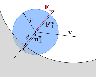
In order to investigate scenarios in which filaments interact with the surrounding environment, we must also account for solid boundaries. By implementing the same approach outlined in the previous section, obstacles and surfaces are modeled as soft boundaries allowing for interpenetration with the elements of the rod (Fig. 7). The wall response 𝐅wsubscriptsuperscript𝐅𝑤perpendicular-to\mathbf{F}^{w}_{\perp} balances the sum of all forces 𝐅subscript𝐅perpendicular-to\mathbf{F}_{\perp} that push the rod against the wall, and is complemented by other two components which help prevent possible interpenetration due to numerics. The interpenetration distance ϵitalic-ϵ\epsilon triggers a normal elastic response proportional to the stiffness of the wall while a dissipative term related to the normal velocity component of the filament with respect to the substrate accounts for a damping force, so that the overall wall response reads

𝐅w=H(ϵ)(𝐅+kwϵγw𝐯𝐮w)𝐮wsubscriptsuperscript𝐅𝑤perpendicular-to𝐻italic-ϵsubscript𝐅perpendicular-tosubscript𝑘𝑤italic-ϵsubscript𝛾𝑤𝐯subscriptsuperscript𝐮𝑤perpendicular-tosubscriptsuperscript𝐮𝑤perpendicular-to\mathbf{F}^{w}_{\perp}=H(\epsilon)\cdot(-\mathbf{F}_{\perp}+k_{w}\epsilon-\gamma_{w}\mathbf{v}\cdot\mathbf{u}^{w}_{\perp})\mathbf{u}^{w}_{\perp} (38)

where H(ϵ)𝐻italic-ϵH(\epsilon) denotes the Heaviside function and ensures that a wall force is produced only in case of contact (ϵ0italic-ϵ0\epsilon\geq 0). Here 𝐮wsubscriptsuperscript𝐮𝑤perpendicular-to\mathbf{u}^{w}_{\perp} is the boundary outward normal (evaluated at the contact point, that is the contact location for which the normal passes through the center of mass of the element), and kwsubscript𝑘𝑤k_{w} and γwsubscript𝛾𝑤\gamma_{w} are, respectively, the wall stiffness and dissipation coefficients.
Refer to caption
Figure 7: Contact model with solid boundaries. Obstacles and surfaces (gray) are modeled as soft boundaries allowing for the interpenetration ϵ=rditalic-ϵ𝑟𝑑\epsilon=r-d with the elements of the filament (blue) characterized by radius r𝑟r and distance d𝑑d from the substrate. The surface normal 𝐮wsubscriptsuperscript𝐮𝑤perpendicular-to\mathbf{u}^{w}_{\perp} determines the direction of the wall’s response 𝐅wsubscriptsuperscript𝐅𝑤perpendicular-to\mathbf{F}^{w}_{\perp} to contact. We note that 𝐅wsubscriptsuperscript𝐅𝑤perpendicular-to\mathbf{F}^{w}_{\perp} balances the sum of all forces 𝐅subscript𝐅perpendicular-to\mathbf{F}_{\perp} that push the rod against the wall, and is complemented by other two components which allow to amend to possible interpenetration due to numerics. These components are an elastic one (kwϵsubscript𝑘𝑤italic-ϵk_{w}\epsilon) and a dissipative one (γw𝐯𝐮wsubscript𝛾𝑤𝐯subscriptsuperscript𝐮𝑤perpendicular-to\gamma_{w}\mathbf{v}\cdot\mathbf{u}^{w}_{\perp}), where kwsubscript𝑘𝑤k_{w} and γwsubscript𝛾𝑤\gamma_{w} are, respectively, the wall stiffness and dissipation coefficients.

IV.0.5 Isotropic and anisotropic surface friction

Solid boundaries also affect the dynamics of the filament through surface friction, a complex physical phenomenon in which a range of factors are involved, from roughness and plasticity of the surfaces in contact to the kinematic initial conditions and geometric setup. Here, we adopt the Amonton-Coulomb model, the simplest of friction models.

This model relates the normal force pushing a body onto a substrate to the friction force through the kinetic μksubscript𝜇𝑘\mu_{k} and static μssubscript𝜇𝑠\mu_{s} friction coefficients, depending on whether the contact surfaces are in relative motion or not.

Despite the simplicity of the model, its formulation and implementation may not necessarily be straightforward, especially in the case of rolling motions. Given the cylindrical geometry of our filaments, the effect of surface friction can be decomposed into a longitudinal component associated with purely translational displacements, and a lateral component associated with both translational and rotational motions (Fig. 8). We use the notation 𝐱subscript𝐱perpendicular-to\mathbf{x}_{\perp}, 𝐱subscript𝐱parallel-to\mathbf{x}_{\parallel}, 𝐱×subscript𝐱\mathbf{x}_{\times} to denote the projection of the vector 𝐱𝐱\mathbf{x} in the directions 𝐮wsubscriptsuperscript𝐮𝑤perpendicular-to\mathbf{u}^{w}_{\perp}, 𝐮wsubscriptsuperscript𝐮𝑤parallel-to\mathbf{u}^{w}_{\parallel}, 𝐮×wsubscriptsuperscript𝐮𝑤\mathbf{u}^{w}_{\times}, as illustrated in Fig. 8.

Refer to caption
Figure 8: Surface friction. (a) The forces produced by friction effects between an element of the rod and the substrate are naturally decomposed into a lateral component in the direction 𝐮w=𝐭×𝐮wsubscriptsuperscript𝐮𝑤parallel-to𝐭subscriptsuperscript𝐮𝑤perpendicular-to\mathbf{u}^{w}_{\parallel}=\mathbf{t}\times\mathbf{u}^{w}_{\perp} and a longitudinal one in the direction 𝐮×w=𝐮w×𝐮wsubscriptsuperscript𝐮𝑤subscriptsuperscript𝐮𝑤perpendicular-tosubscriptsuperscript𝐮𝑤parallel-to\mathbf{u}^{w}_{\times}=\mathbf{u}^{w}_{\perp}\times\mathbf{u}^{w}_{\parallel}. We note that in general 𝐮×w𝐭subscriptsuperscript𝐮𝑤𝐭\mathbf{u}^{w}_{\times}\neq\mathbf{t}. The notation 𝐱subscript𝐱perpendicular-to\mathbf{x}_{\perp}, 𝐱subscript𝐱parallel-to\mathbf{x}_{\parallel}, 𝐱×subscript𝐱\mathbf{x}_{\times} denotes the projection of the vector 𝐱𝐱\mathbf{x} in the directions 𝐮wsubscriptsuperscript𝐮𝑤perpendicular-to\mathbf{u}^{w}_{\perp}, 𝐮wsubscriptsuperscript𝐮𝑤parallel-to\mathbf{u}^{w}_{\parallel}, 𝐮×wsubscriptsuperscript𝐮𝑤\mathbf{u}^{w}_{\times}. (b,c) Kinematic and dynamic quantities at play at any cross section in case of rolling and slipping (b) and pure rolling (c) motion. Red arrows correspond to forces and torques, green arrows correspond to velocities, and black arrows correspond to geometric quantities.

The longitudinal friction force 𝐅longsubscript𝐅𝑙𝑜𝑛𝑔\mathbf{F}_{long} is opposite to either the resultant of all forces 𝐅×subscript𝐅\mathbf{F}_{\times} acting on an element (static case) or to the translational velocity 𝐯×subscript𝐯\mathbf{v}_{\times} (kinetic case) along the direction 𝐮×wsubscriptsuperscript𝐮𝑤\mathbf{u}^{w}_{\times} (Fig. 8). The Amonton-Coulomb model then reads

𝐅long={max(|𝐅×|,μs|𝐅|)𝐅×|𝐅×|if |𝐯×|vϵμk|𝐅|𝐯×|𝐯×|if |𝐯×|>vϵ,subscript𝐅𝑙𝑜𝑛𝑔casessubscript𝐅subscript𝜇𝑠subscript𝐅perpendicular-tosubscript𝐅subscript𝐅if subscript𝐯subscript𝑣italic-ϵsubscript𝜇𝑘subscript𝐅perpendicular-tosubscript𝐯subscript𝐯if subscript𝐯subscript𝑣italic-ϵ\mathbf{F}_{long}=\begin{dcases}-\max(|\mathbf{F}_{\times}|,\mu_{s}|\mathbf{F}_{\perp}|)\cdot\frac{\mathbf{F}_{\times}}{|\mathbf{F}_{\times}|}&\text{if }|\mathbf{v}_{\times}|\leq v_{\epsilon}\\ -\mu_{k}|\mathbf{F}_{\perp}|\cdot\frac{\mathbf{v}_{\times}}{|\mathbf{v}_{\times}|}&\text{if }|\mathbf{v}_{\times}|>v_{\epsilon}\end{dcases},

where vϵ0subscript𝑣italic-ϵ0v_{\epsilon}\rightarrow 0 is the absolute velocity threshold value employed to distinguish between static (|𝐯×|vϵsubscript𝐯subscript𝑣italic-ϵ|\mathbf{v}_{\times}|\leq v_{\epsilon}) and kinetic (|𝐯×|>vϵsubscript𝐯subscript𝑣italic-ϵ|\mathbf{v}_{\times}|>v_{\epsilon}) case. We define vϵsubscript𝑣italic-ϵv_{\epsilon} in a limit form to accommodate the fact that inequalities are numerically evaluated up to a small threshold value. The static friction force is always equal and opposite to 𝐅×subscript𝐅\mathbf{F}_{\times} up to a maximum value proportional to the normal force |𝐅|subscript𝐅perpendicular-to|\mathbf{F}_{\perp}| though the coefficient μssubscript𝜇𝑠\mu_{s}. The kinetic friction force is instead opposite to the translational velocity 𝐯×subscript𝐯\mathbf{v}_{\times}, but does not depend on its actual magnitude and is proportional to |𝐅|subscript𝐅perpendicular-to|\mathbf{F}_{\perp}| via μksubscript𝜇𝑘\mu_{k}. In general μs>μksubscript𝜇𝑠subscript𝜇𝑘\mu_{s}>\mu_{k}, so that it is harder to set a body into motion from rest than to drag it.

The lateral displacement of a filament in the direction 𝐮w=𝐮×w×𝐮wsubscriptsuperscript𝐮𝑤parallel-tosubscriptsuperscript𝐮𝑤subscriptsuperscript𝐮𝑤perpendicular-to\mathbf{u}^{w}_{\parallel}=\mathbf{u}^{w}_{\times}\times\mathbf{u}^{w}_{\perp} is associated with both translational (𝐯subscript𝐯parallel-to\mathbf{v}_{\parallel}) and rotational (𝝎×=ω×𝐮×wsubscript𝝎subscript𝜔subscriptsuperscript𝐮𝑤\boldsymbol{\omega}_{\times}=\omega_{\times}\mathbf{u}^{w}_{\times}) motions, as illustrated in Fig. 8b,c. In this case the distinction between static and kinetic friction does not depend on 𝐯subscript𝐯parallel-to\mathbf{v}_{\parallel}, but on the relative velocity (also referred to as slip velocity) between the rod and the substrate

𝐯slip=𝐯+𝐯cont,𝐯cont=r𝐮w×𝝎×,formulae-sequencesubscript𝐯𝑠𝑙𝑖𝑝subscript𝐯parallel-tosubscript𝐯𝑐𝑜𝑛𝑡subscript𝐯𝑐𝑜𝑛𝑡𝑟subscriptsuperscript𝐮𝑤perpendicular-tosubscript𝝎\mathbf{v}_{slip}=\mathbf{v}_{\parallel}+\mathbf{v}_{cont},~{}~{}~{}~{}~{}\mathbf{v}_{cont}=r\mathbf{u}^{w}_{\perp}\times\boldsymbol{\omega}_{\times}, (39)

where 𝐯contsubscript𝐯𝑐𝑜𝑛𝑡\mathbf{v}_{cont} is the local velocity of the filament at the contact point with the substrate, due to the axial component of the angular velocity 𝝎×subscript𝝎\boldsymbol{\omega}_{\times}.

In the static or no-slip scenario (𝐯slip=𝟎subscript𝐯𝑠𝑙𝑖𝑝0\mathbf{v}_{slip}=\mathbf{0}), the linear momentum balance in the direction 𝐮wsubscriptsuperscript𝐮𝑤parallel-to\mathbf{u}^{w}_{\parallel}, and the angular momentum balance about the axis 𝐮×wsubscriptsuperscript𝐮𝑤\mathbf{u}^{w}_{\times} express a kinematic constraint between the linear acceleration a𝐮w𝑎subscriptsuperscript𝐮𝑤parallel-toa\mathbf{u}^{w}_{\parallel} and angular acceleration 𝝎×=(𝐮w×a𝐮w)/rsubscript𝝎subscriptsuperscript𝐮𝑤perpendicular-to𝑎subscriptsuperscript𝐮𝑤parallel-to𝑟\boldsymbol{\omega}_{\times}=(\mathbf{u}^{w}_{\perp}\times a\mathbf{u}^{w}_{\parallel})/r, so that

(F+Froll)𝐮wsubscript𝐹parallel-tosubscript𝐹𝑟𝑜𝑙𝑙subscriptsuperscript𝐮𝑤parallel-to\displaystyle(F_{\parallel}+F_{roll})\mathbf{u}^{w}_{\parallel} =\displaystyle= dma𝐮w𝑑𝑚𝑎subscriptsuperscript𝐮𝑤parallel-to\displaystyle dm\cdot a\mathbf{u}^{w}_{\parallel} (40)
T×𝐮×wr𝐮w×Froll𝐮wsubscript𝑇subscriptsuperscript𝐮𝑤𝑟subscriptsuperscript𝐮𝑤perpendicular-tosubscript𝐹𝑟𝑜𝑙𝑙subscriptsuperscript𝐮𝑤parallel-to\displaystyle T_{\times}\mathbf{u}^{w}_{\times}-r\mathbf{u}^{w}_{\perp}\times F_{roll}\mathbf{u}^{w}_{\parallel} =\displaystyle= J𝐮w×a𝐮wr,𝐽subscriptsuperscript𝐮𝑤perpendicular-to𝑎subscriptsuperscript𝐮𝑤parallel-to𝑟\displaystyle J\cdot\frac{\mathbf{u}^{w}_{\perp}\times a\mathbf{u}^{w}_{\parallel}}{r}, (41)

where 𝐅=F𝐮wsubscript𝐅parallel-tosubscript𝐹parallel-tosubscriptsuperscript𝐮𝑤parallel-to\mathbf{F}_{\parallel}=F_{\parallel}\mathbf{u}^{w}_{\parallel} and 𝐓×=T×𝐮×wsubscript𝐓subscript𝑇subscriptsuperscript𝐮𝑤\mathbf{T}_{\times}=T_{\times}\mathbf{u}^{w}_{\times} are the forces and torques acting on the local element, and 𝐅roll=Froll𝐮wsubscript𝐅𝑟𝑜𝑙𝑙subscript𝐹𝑟𝑜𝑙𝑙subscriptsuperscript𝐮𝑤parallel-to\mathbf{F}_{roll}=F_{roll}\mathbf{u}^{w}_{\parallel} is the rolling friction force at the substrate-filament interface necessary to meet the no-slip condition. By recalling that a disk mass second moment of inertia about 𝐮×wsubscriptsuperscript𝐮𝑤\mathbf{u}^{w}_{\times} is J=r2dm/2𝐽superscript𝑟2𝑑𝑚2J=r^{2}dm/2, the above system can be solved for the unknown a𝑎a and Frollsubscript𝐹𝑟𝑜𝑙𝑙F_{roll}, yielding

𝐅roll=rF2T×3r𝐮w.subscript𝐅𝑟𝑜𝑙𝑙𝑟subscript𝐹parallel-to2subscript𝑇3𝑟subscriptsuperscript𝐮𝑤parallel-to\mathbf{F}_{roll}=-\frac{rF_{\parallel}-2T_{\times}}{3r}\mathbf{u}^{w}_{\parallel}. (42)

Therefore the lateral friction force 𝐅latsubscript𝐅𝑙𝑎𝑡\mathbf{F}_{lat} and the associate torque 𝐂latsubscriptsuperscript𝐂𝑙𝑎𝑡\mathbf{C}^{lat}_{\mathcal{L}} can be finally expressed as

𝐅lat={max(|𝐅roll|,μsr|𝐅|)𝐅roll|𝐅roll|if |𝐯slip|vϵμkr|𝐅|𝐯slip|𝐯slip|if |𝐯slip|>vϵ,𝐂lat=𝐐(𝐅lat×r𝐮w),formulae-sequencesubscript𝐅𝑙𝑎𝑡casessubscript𝐅𝑟𝑜𝑙𝑙subscriptsuperscript𝜇𝑟𝑠subscript𝐅perpendicular-tosubscript𝐅𝑟𝑜𝑙𝑙subscript𝐅𝑟𝑜𝑙𝑙if subscript𝐯𝑠𝑙𝑖𝑝subscript𝑣italic-ϵsubscriptsuperscript𝜇𝑟𝑘subscript𝐅perpendicular-tosubscript𝐯𝑠𝑙𝑖𝑝subscript𝐯𝑠𝑙𝑖𝑝if subscript𝐯𝑠𝑙𝑖𝑝subscript𝑣italic-ϵsubscriptsuperscript𝐂𝑙𝑎𝑡𝐐subscript𝐅𝑙𝑎𝑡𝑟superscriptsubscript𝐮perpendicular-to𝑤\mathbf{F}_{lat}=\begin{dcases}\max(|\mathbf{F}_{roll}|,\mu^{r}_{s}|\mathbf{F}_{\perp}|)\cdot\frac{\mathbf{F}_{roll}}{|\mathbf{F}_{roll}|}&\text{if }|\mathbf{v}_{slip}|\leq v_{\epsilon}\\ -\mu^{r}_{k}|\mathbf{F}_{\perp}|\cdot\frac{\mathbf{v}_{slip}}{|\mathbf{v}_{slip}|}&\text{if }|\mathbf{v}_{slip}|>v_{\epsilon}\end{dcases},~{}~{}~{}~{}~{}~{}~{}~{}\mathbf{C}^{lat}_{\mathcal{L}}=\mathbf{Q}(\mathbf{F}_{lat}\times r\mathbf{u}_{\perp}^{w}),

where μsrsuperscriptsubscript𝜇𝑠𝑟\mu_{s}^{r} and μkrsuperscriptsubscript𝜇𝑘𝑟\mu_{k}^{r} are, respectively, the rolling static and kinetic friction coefficients.

So far we have considered isotropic friction by assuming that the coefficients μssubscript𝜇𝑠\mu_{s} and μksubscript𝜇𝑘\mu_{k} are constant and independent from the direction of the total acting forces (static case) or relative velocities (kinetic case). Nevertheless, frictional forces may be highly anisotropic. For example, the anisotropy caused by the presence of scales on the body of a snake crucially affects gaits and performance Guo:2008 ; Hu:2009 .

The Amonton-Coulomb model can be readily extended to account for anisotropic effects by simply assuming the friction coefficients μssubscript𝜇𝑠\mu_{s} and μksubscript𝜇𝑘\mu_{k} to be functions of a given reference direction. The nature of these functions depends on the specific physical problems under investigation. An example of this approach is illustrated in Section V.0.2 in the context of limbless locomotion. Isotropic and anisotropic friction validation benchmarks are presented in the Appendix.

IV.0.6 Hydrodynamics

We also extend our computational framework to address flow-structure interaction problems. In particular we consider the case in which viscous forces dominate over inertial effects, i.e. we consider systems in which the Reynolds number Re=ρfUL/μ1𝑅𝑒subscript𝜌𝑓𝑈𝐿𝜇much-less-than1Re=\rho_{f}UL/\mu\ll 1 where ρfsubscript𝜌𝑓\rho_{f} and μ𝜇\mu are the density and dynamic viscosity of the fluid, and U𝑈U is the characteristic velocity of the rod. Under these conditions, the drag forces exerted by the fluid on our filaments can be determined analytically within the context of slender-body theory Cox:1970 ; Lauga:2009 . At leading order resistive force line densities scale linearly with the local rod velocities 𝐯𝐯\mathbf{v} according to

𝐟H=4πμln(L/r)(𝐈12𝐭T𝐭)𝐯.superscript𝐟𝐻4𝜋𝜇𝐿𝑟𝐈12superscript𝐭𝑇𝐭𝐯\mathbf{f}^{H}=-\frac{4\pi\mu}{\ln(L/r)}\left(\mathbf{I}-\frac{1}{2}\mathbf{t}^{T}\mathbf{t}\right)\mathbf{v}. (43)

We note that the matrix (𝐈12𝐭T𝐭)𝐈12superscript𝐭𝑇𝐭(\mathbf{I}-\frac{1}{2}\mathbf{t}^{T}\mathbf{t}) introduces an anisotropic effect for which

𝐟H=2πμln(L/r)|(𝐯𝐭)𝐭|,𝐟H=4πμln(L/r)|𝐯(𝐯𝐭)𝐭|formulae-sequencesubscriptsuperscript𝐟𝐻parallel-to2𝜋𝜇𝐿𝑟𝐯𝐭𝐭subscriptsuperscript𝐟𝐻perpendicular-to4𝜋𝜇𝐿𝑟𝐯𝐯𝐭𝐭\mathbf{f}^{H}_{\parallel}=-\frac{2\pi\mu}{\ln(L/r)}|(\mathbf{v}\cdot\mathbf{t})\mathbf{t}|,~{}~{}~{}~{}~{}\mathbf{f}^{H}_{\perp}=-\frac{4\pi\mu}{\ln(L/r)}|\mathbf{v}-(\mathbf{v}\cdot\mathbf{t})\mathbf{t}| (44)

where 𝐟H=(𝐟H𝐭)𝐭subscriptsuperscript𝐟𝐻parallel-tosuperscript𝐟𝐻𝐭𝐭\mathbf{f}^{H}_{\parallel}=(\mathbf{f}^{H}\cdot\mathbf{t})\mathbf{t} and 𝐟H=𝐟H𝐟Hsubscriptsuperscript𝐟𝐻perpendicular-tosuperscript𝐟𝐻subscriptsuperscript𝐟𝐻parallel-to\mathbf{f}^{H}_{\perp}=\mathbf{f}^{H}-\mathbf{f}^{H}_{\parallel} are, respectively, tangential and orthogonal viscous drag components. The coupling of liquid environment, filament mechanics and muscular activity provides a flexible platform to characterize biological locomotion at the microscopic scale (bacteria, protozoa, algae, etc.) and to design propulsion strategies in the context of artificial micro-swimmers Williams:2014 ; Park:2016 .

V Applications

We now proceed to illustrate the potential of our framework with three different applications. We consider first a static problem in which self-contact, bending and twist give rise to the classic out-of-plane configurations denoted as plectonemes Ghatak:2005 , while the addition of stretching and shearing produces a different type of experimentally observed solutions, known as solenoids Ghatak:2005 . Then we turn our attention to two dynamic biophysical problems in which an active filament interacts with a solid and a liquid environment, exhibiting qualitatively different optimal biolocomotion strategies.

V.0.1 Plectonemes and solenoids

When an inextensible rod is clamped at one end and twisted a sufficiently large number of times at the other end, it becomes unstable, coils up and generates a characteristic structure known as a plectoneme Thompson:1996 . While this behavior has been well characterized both theoretically and experimentally Thompson:1996 , its analog for highly extensible filaments has been ignored. In particular, for large extensional and twisting strains qualitatively different solutions arise, such as those corresponding to tightly packed solenoidal structures Ghatak:2005 whose properties are as yet poorly understood.
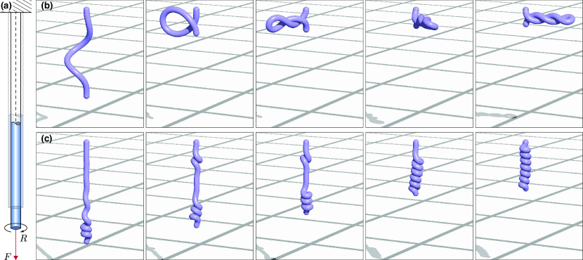
Refer to caption
Figure 9: Formation of plectonemes and solenoids. (a) We consider a soft rod clamped at one end, subject to a constant vertical load F𝐹F and twisted R𝑅R times at the other end. (b) Formation of a plectoneme for F=0𝐹0F=0 (leading to the total elongation L/L^1𝐿^𝐿1L/\hat{L}\approx 1) and R=4𝑅4R=4. (c) Formation of a solenoid for F=300𝐹300F=300 N (leading to the total elongation L/L^1.15𝐿^𝐿1.15L/\hat{L}\approx 1.15) and R=13𝑅13R=13. Settings: length L=1𝐿1L=1 m, radius r=0.025𝑟0.025r=0.025 m, mass m=1𝑚1m=1 kg, Young’s modulus E=106𝐸superscript106E=10^{6} Pa, shear modulus G=2E/3𝐺2𝐸3G=2E/3 Pa, shear/stretch matrix 𝐒^=diag(4GA^/3,4GA^/3,EA^)^𝐒diag4𝐺^𝐴34𝐺^𝐴3𝐸^𝐴\hat{\mathbf{S}}=\text{diag}(4G\hat{A}/3,4G\hat{A}/3,E\hat{A}) N, bend/twist matrix 𝐁^=diag(EI1,EI2,GI3)^𝐁diag𝐸subscript𝐼1𝐸subscript𝐼2𝐺subscript𝐼3\hat{\mathbf{B}}=\text{diag}(EI_{1},EI_{2},GI_{3}) Nm2, dissipation constant γ=2𝛾2\gamma=2 kg/(ms), ksc=104subscript𝑘𝑠𝑐superscript104k_{sc}=10^{4} kg/s2, γsc=10subscript𝛾𝑠𝑐10\gamma_{sc}=10 kg/s, discretization elements n=100𝑛100n=100, timestep δt=0.01δl𝛿𝑡0.01𝛿𝑙\delta t=0.01\delta l s, Ttwist=75subscript𝑇twist75T_{\text{twist}}=75 s, Trelax=50subscript𝑇relax50T_{\text{relax}}=50 s.

Given the broad scope of our computational framework for the investigation of soft filament dynamics, we can now study the formation of both solenoids and plectonemes. As illustrated in Fig. 9a, a soft rod of Young’s modulus E=106𝐸superscript106E=10^{6} Pa is clamped at one end, and subject to an axial load F𝐹F, while also being twisted R𝑅R times at the other end. As experimentally and theoretically observed for F=0𝐹0F=0, i.e. in the absence of stretching (L/L^1𝐿^𝐿1L/\hat{L}\approx 1), plectonemes are generated (Fig. 9b). When the load F𝐹F is increased so that the elongation of the rod approaches L/L^1.15𝐿^𝐿1.15L/\hat{L}\approx 1.15, solenoids arise as predicted in Ghatak:2005 and illustrated in Fig. 9c. This test case, therefore, shows the ability of our solver to capture qualitatively different instability mechanisms, driven by the competition between the different modes of deformation of the rod. We leave the details of the explanation of the phase diagram for the formation of plectonemes, solenoids and intermediate structures Ghatak:2005 for a later study.

V.0.2 Slithering

The mechanics of slithering locomotion typical of snakes has been extensively investigated experimentally Gray:1950 ; Hu:2009 ; Transeth:2009 , theoretically Gray:1946 ; Guo:2008 ; Alben:2013 and computationally Erkmen:2002 ; Tanev:2005 . While biological experiments have provided quantitative insights, theoretical and computational models have been instrumental to characterize qualitatively the working principles underlying snake locomotion. Although these models implement different levels of realism, they generally rely on a number of key simplifications. Typically, theoretical models assume planar deformations Guo:2008 and/or disregard mechanics by prescribing body kinematics Alben:2013 . Computational models offer a more realistic representation, but they have mostly been developed for and tailored to robotic applications Erkmen:2002 ; Tanev:2005 . For example, snakes are often modeled as a relatively small set of hinges and/or springs representing pointwise localized actuators that connect contiguous rigid segments. Therefore, they do not account for the continuum nature of elastic body mechanics and biological muscular activity. Moreover, in robot replicas the critical feature of friction anisotropy is commonly achieved through the use of wheels Transeth:2009 . As a consequence computational models often assume only two sources of anisotropy, in the tangential and lateral direction with respect to the body. This is in contrast with biological experiments Hu:2009 that highlight the importance of all three sources of anisotropy, namely forward, backward and lateral.
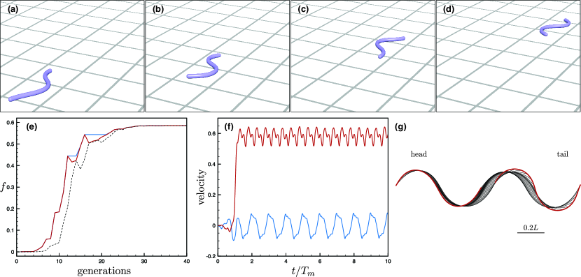
Refer to caption
Figure 10: Optimal lateral undulation gait. (a, b, c, d) Instances at different times of a snake characterized by the identified optimal gait. (e) Evolution of the fitness function f=vmaxfwd𝑓subscriptsuperscript𝑣fwdmaxf=v^{\text{fwd}}_{\text{max}} as function of the number of generations produced by CMA-ES. Solid blue, solid red and dashed black lines represent, respectively, the evolution of f𝑓f corresponding to the best solution, the best solution within the current generation, and the mean generation value. (f) Scaled forward (red) and lateral (blue) center of mass velocities versus normalized time. (g) Gait envelope over one oscillation period Tmsubscript𝑇𝑚T_{m}. Red lines represent head and tail displacement in time. Settings: Froude number Fr=0.1𝐹𝑟0.1Fr=0.1, length L=1𝐿1L=1 m, radius r=0.025𝑟0.025r=0.025 m, density ρ=103𝜌superscript103\rho=10^{3} kg/m3, Tm=1subscript𝑇𝑚1T_{m}=1 s, Young’s modulus E=107𝐸superscript107E=10^{7} Pa, shear modulus G=2E/3𝐺2𝐸3G=2E/3 Pa, shear/stretch matrix 𝐒^=diag(4GA^/3,4GA^/3,EA^)^𝐒diag4𝐺^𝐴34𝐺^𝐴3𝐸^𝐴\hat{\mathbf{S}}=\text{diag}(4G\hat{A}/3,4G\hat{A}/3,E\hat{A}) N, bend/twist matrix 𝐁^=diag(EI1,EI2,GI3)^𝐁diag𝐸subscript𝐼1𝐸subscript𝐼2𝐺subscript𝐼3\hat{\mathbf{B}}=\text{diag}(EI_{1},EI_{2},GI_{3}) Nm2, dissipation constant γ=5𝛾5\gamma=5 kg/(ms), gravity g=9.81𝑔9.81g=9.81 m/s2, friction coefficient ratios μkf:μkb:μkr=1:1.5:2:subscriptsuperscript𝜇𝑓𝑘subscriptsuperscript𝜇𝑏𝑘:subscriptsuperscript𝜇𝑟𝑘1:1.5:2\mu^{f}_{k}:\mu^{b}_{k}:\mu^{r}_{k}=1:1.5:2 and μsf:μsb:μsr=1:1.5:2:subscriptsuperscript𝜇𝑓𝑠subscriptsuperscript𝜇𝑏𝑠:subscriptsuperscript𝜇𝑟𝑠1:1.5:2\mu^{f}_{s}:\mu^{b}_{s}:\mu^{r}_{s}=1:1.5:2 with μsf=2μkfsubscriptsuperscript𝜇𝑓𝑠2subscriptsuperscript𝜇𝑓𝑘\mu^{f}_{s}=2\mu^{f}_{k}, friction threshold velocity vϵ=108subscript𝑣italic-ϵsuperscript108v_{\epsilon}=10^{-8} m/s, ground stiffness and viscous dissipation kw=1subscript𝑘𝑤1k_{w}=1 kg/s2 and γw=106subscript𝛾𝑤superscript106\gamma_{w}=10^{-6} kg/s, discretization elements n=50𝑛50n=50, timestep δt=2.5105Tm𝛿𝑡2.5superscript105subscript𝑇𝑚\delta t=2.5\cdot 10^{-5}~{}T_{m}, wavelength λm=0.97Lsubscript𝜆𝑚0.97𝐿\lambda_{m}=0.97L, phase shift ϕm=0subscriptitalic-ϕ𝑚0\phi_{m}=0, torque B-spline coefficients βi=0,,5={0,17.4,48.5,5.4,14.7,0}subscript𝛽𝑖05017.448.55.414.70\beta_{i=0,\dots,5}=\{0,17.4,48.5,5.4,14.7,0\} Nm, bounds maximum attainable torque |β|i=0,,5max=50subscriptsuperscript𝛽max𝑖0550|\beta|^{\text{max}}_{i=0,\dots,5}=50 Nm.

Our approach complements these previous attempts by accounting for physical and biological effects within a continuum framework (Eqs. 12-15). In this section we demonstrate the qualitative and quantitative capabilities of the proposed method by reverse engineering optimal slithering gaits that maximize forward speed.

We consider a soft filament of unit length actuated via a planar traveling torque wave of muscular activity in the direction perpendicular to the ground. The interaction with the substrate is characterized by the ratios μkf:μkb:μkr=1:1.5:2:subscriptsuperscript𝜇𝑓𝑘subscriptsuperscript𝜇𝑏𝑘:subscriptsuperscript𝜇𝑟𝑘1:1.5:2\mu^{f}_{k}:\mu^{b}_{k}:\mu^{r}_{k}=1:1.5:2 and μsf:μsb:μsr=1:1.5:2:subscriptsuperscript𝜇𝑓𝑠subscriptsuperscript𝜇𝑏𝑠:subscriptsuperscript𝜇𝑟𝑠1:1.5:2\mu^{f}_{s}:\mu^{b}_{s}:\mu^{r}_{s}=1:1.5:2 with μsf=2μkfsubscriptsuperscript𝜇𝑓𝑠2subscriptsuperscript𝜇𝑓𝑘\mu^{f}_{s}=2\mu^{f}_{k}, as experimentally observed for juvenile Pueblan milk snakes on a moderately rough surface Hu:2009 . The value of the friction coefficient μkfsuperscriptsubscript𝜇𝑘𝑓\mu_{k}^{f} is set so that the ratio between inertial and friction forces captured by the Froude number is Fr=(L/Tm2)/(μkfg)=0.1𝐹𝑟𝐿superscriptsubscript𝑇𝑚2subscriptsuperscript𝜇𝑓𝑘𝑔0.1Fr=(L/T_{m}^{2})/(\mu^{f}_{k}g)=0.1, as measured for these snakes Hu:2009 .

In the spirit of Gazzola:2012 ; Rees:2013 ; Rees:2015 , we wish to identify the fastest gaits by optimizing the filament muscular activity. The torque wave generated by the snake is parameterized according to Section IV.0.2 and is characterized by Nm=6subscript𝑁𝑚6N_{m}=6 control points and a unit oscillation period Tmsubscript𝑇𝑚T_{m}, so that overall we optimize for five parameters, four of which are responsible for the torque profile along the rod (β1subscript𝛽1\beta_{1}, β2subscript𝛽2\beta_{2}, β3subscript𝛽3\beta_{3}, β4subscript𝛽4\beta_{4}), while the last one represents the wavenumber 2π/λm2𝜋subscript𝜆𝑚2\pi/\lambda_{m} (see Section IV.0.2).

These parameters are left free to evolve from an initial zero value, guided by an automated optimization procedure that identifies the optimal values that maximize the snake’s forward average speed vmaxfwdsubscriptsuperscript𝑣fwdmaxv^{\text{fwd}}_{\text{max}} over one activation cycle Tmsubscript𝑇𝑚T_{m}. The algorithm of choice is the Covariance Matrix Adaptation - Evolution StrategyHansen:2001 ; Hansen:2003 (CMA-ES) which has been proven effective in a range of biophysical and engineering problems, from the optimization of swimming gaits Gazzola:2012 , morphologies Rees:2013 ; Rees:2015 and collective dynamics Gazzola:2015a to the identification of aircraft alleviation schemes Chatelain:2011 or virus traffic mechanisms Gazzola:2009 . The CMA-ES is a stochastic optimization algorithm that samples generations of p𝑝p parameter vectors from a multivariate Gaussian distribution 𝒩𝒩\mathcal{N}. Here each parameter vector represents a muscular activation instance, and every generation entails the evaluation of p=60𝑝60p=60 different gaits. The covariance matrix of the distribution 𝒩𝒩\mathcal{N} is then adapted based on successful past gaits, chosen according to their corresponding cost function value f=vmaxfwd𝑓subscriptsuperscript𝑣fwdmaxf=v^{\text{fwd}}_{\text{max}}, until convergence to the optimum.

The course of the optimization is reported in Fig. 10 together with the kinematic details of the identified fastest gait. As can be noticed in Fig. 10e,f the forward scaled average speed approaches vmaxfwd0.6similar-to-or-equalssubscriptsuperscript𝑣fwdmax0.6v^{\text{fwd}}_{\text{max}}\simeq 0.6, consistent with experimental evidence Shine:2003 . Moreover, CMA-ES finds that the optimal wavelength is λmLsimilar-to-or-equalssubscript𝜆𝑚𝐿\lambda_{m}\simeq L (Fig. 10g), again consistent with biological observations Hu:2009 ; Goldman:2010 . Thus, this value of wavelength strikes a balance between thrust production and drag minimization within the mechanical constraints of the system.

We note that a rigorous characterization of slithering locomotion would require the knowledge of a number of biologically relevant parameters (Young’s and shear moduli of muscular tissue, maximum attainable torques, etc) and environmental conditions (terrain asperities, presence of pegs, etc) and goes beyond the scope of the present work. Nevertheless, this study illustrates the robustness, quantitative accuracy and suitability of our methodology for the characterization of bio-locomotion phenomena.

V.0.3 Swimming

We finally turn to apply the inverse design approach outlined in the previous section to the problem of swimming at low Reynolds numbers where viscous forces dominate inertial effects. We maintain the exact same set up as in the slithering case, while we change the environment from a solid substrate to a viscous fluid. The flow-filament interaction is then modeled via slender-body theory, as illustrated in Section IV.0.6.

Once again we inverse design planar optimal gaits for forward average speed f=vmaxfwd𝑓subscriptsuperscript𝑣fwdmaxf=v^{\text{fwd}}_{\text{max}} within one activation cycle Tmsubscript𝑇𝑚T_{m}, by employing the same muscular activity parameterization as for slithering. In order to verify a-posteriori the biological relevance of the identified optimal solution, we consider the case of the sea urchin spermatozoon Echinus esculentus Woolley:2001 which swims by means of helical or planar waves traveling along its flagella of length Ls40similar-to-or-equalssubscript𝐿𝑠40L_{s}\simeq 40 μ𝜇\mum. The gait corresponding to planar swimming is characterized by kinematic undulations of wavelength λs<Lssubscript𝜆𝑠subscript𝐿𝑠\lambda_{s}<L_{s} and frequency fs2.8similar-to-or-equalssubscript𝑓𝑠2.8f_{s}\simeq 2.8. At Re104similar-to-or-equals𝑅𝑒superscript104Re\simeq 10^{-4} the spermatozoon attains the scaled velocity vs=Us/(fsLs)0.08±0.03subscript𝑣𝑠subscript𝑈𝑠subscript𝑓𝑠subscript𝐿𝑠similar-to-or-equalsplus-or-minus0.080.03v_{s}=U_{s}/(f_{s}L_{s})\simeq 0.08\pm 0.03, where Ussubscript𝑈𝑠U_{s} is the dimensional cruise speed Woolley:2001 . Although this gait may not be the absolute optimal planar locomotion pattern, the fact that it is replicated in a large number of organisms Lauga:2009 suggests that it captures some effective features that we expect to qualitatively recover via our numerical optimization.
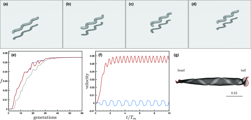
Refer to caption
Figure 11: Optimal planar swimming gait at low Reynolds number. (a, b, c, d) Instances at different times of a filament swimming according to the identified optimal gait. (e) Evolution of the fitness function f=vmaxfwd𝑓subscriptsuperscript𝑣fwdmaxf=v^{\text{fwd}}_{\text{max}} as function of the number of generations produced by CMA-ES. Solid blue, solid red and dashed black lines represent, respectively, the evolution of f𝑓f corresponding to the best solution, the best solution within the current generation, and the mean generation value. (f) Scaled forward (red) and lateral (blue) center of mass velocities versus normalized time. (g) Gait envelope over one oscillation period Tmsubscript𝑇𝑚T_{m}. Red lines represent head and tail displacement in time. Settings: Reynolds number Re=104𝑅𝑒superscript104Re=10^{-4}, length L=1𝐿1L=1 m, radius r=0.025𝑟0.025r=0.025 m, filament density ρ=103𝜌superscript103\rho=10^{3} kg/m3, Tm=1subscript𝑇𝑚1T_{m}=1 s, Young’s modulus E=107𝐸superscript107E=10^{7} Pa, shear modulus G=2E/3𝐺2𝐸3G=2E/3 Pa, shear/stretch matrix 𝐒^=diag(4GA^/3,4GA^/3,EA^)^𝐒diag4𝐺^𝐴34𝐺^𝐴3𝐸^𝐴\hat{\mathbf{S}}=\text{diag}(4G\hat{A}/3,4G\hat{A}/3,E\hat{A}) N, bend/twist matrix 𝐁^=diag(EI1,EI2,GI3)^𝐁diag𝐸subscript𝐼1𝐸subscript𝐼2𝐺subscript𝐼3\hat{\mathbf{B}}=\text{diag}(EI_{1},EI_{2},GI_{3}) Nm2, dissipation constant γ=5𝛾5\gamma=5 kg/(ms), discretization elements n=50𝑛50n=50, timestep δt=2.5105Tm𝛿𝑡2.5superscript105subscript𝑇𝑚\delta t=2.5\cdot 10^{-5}~{}T_{m}, wavelength λm=2.6Lsubscript𝜆𝑚2.6𝐿\lambda_{m}=2.6L, phase shift ϕm=0subscriptitalic-ϕ𝑚0\phi_{m}=0, torque B-spline coefficients βi=0,,5={0,50,50,50,50,0}subscript𝛽𝑖050505050500\beta_{i=0,\dots,5}=\{0,50,50,50,50,0\} Nm, bounds maximum attainable torque |β|i=0,,5max=50subscriptsuperscript𝛽max𝑖0550|\beta|^{\text{max}}_{i=0,\dots,5}=50 Nm.

The course of the optimization is reported in Fig. 11 together with the kinematic details of the identified fastest gait. As can be noticed in Fig. 11e,f the forward average scaled speed and wavelength approach vmaxfwd0.055similar-to-or-equalssubscriptsuperscript𝑣fwdmax0.055v^{\text{fwd}}_{\text{max}}\simeq 0.055 and λm0.38Lsimilar-to-or-equalssubscript𝜆𝑚0.38𝐿\lambda_{m}\simeq 0.38L, qualitatively and quantitatively consistent with experimental evidence Woolley:2001 .

As in the previous section, we note that a rigorous characterization of swimming at low Reynolds numbers would require the knowledge of a number of biologically relevant parameters and environmental conditions, and goes beyond the scope of the present work. Nevertheless, this and the previous study illustrate how the interplay between filament mechanics and the surrounding environment crucially affects propulsive gaits, as is biologically evident and automatically recovered via our numerical inverse design approach.

VI Conclusions

We have presented a robust and flexible framework for the simulation of soft filaments deforming in three dimensional space. Our scheme accounts at any given cross section for all possible deformation degrees of freedom, namely normal and orthonormal bending, twisting, stretching and shearing. Furthermore, we enhance it to handle self-contact, muscular activity, solid boundaries, isotropic and anisotropic friction as well as hydrodynamics. The outcome is a relatively simple algorithm able to simulate a plethora of physical and biological phenomena.

We validate the proposed method against a battery of benchmark problems entailing different physical aspects and boundary conditions, and we examine its convergence properties in depth. We further showcase the capabilities of our approach by studying several applications: the formation of solenoids and plectonemes and the evolutionary optimization of terrestrial limbless locomotion and swimming. We emphasize that using an evolutionary strategy in combination with a numerical solver severely tests the robustness of the solver itself, due to the variety of candidate solutions produced throughout the process.

Therefore, our results demonstrate the robustness and accuracy of our discrete model under a variety of different deformation regimes and illustrate its flexibility and potential for a wide range of passive and active applications involving soft filaments.

Ongoing work involves its coupling to realistic high Reynolds number flow solvers Gazzola:2011a as well as its integration with sensory feedback models for the characterization of locomotory neural circuitry Gazzola:2015 .

Acknowledgements

We thank Nicholas Charles for a careful reading of and comments on the paper. We thank the Blue Waters project (OCI-0725070, ACI-1238993), a joint effort of the University of Illinois at Urbana-Champaign and its National Center for Supercomputing Applications, for partial support (MG).

Appendix A Lagrangian governing equations

The following shows the conversion of governing equations for unstretchable filaments from the lab to material frame of reference. Note that in the Governing Equations and Numerical Methods sections of the main text all terms are scaled appropriately by the local dilatation to account for stretching.

The time and space derivatives of the centerline 𝐫(s,t)𝐫𝑠𝑡\mathbf{r}(s,t) are associated with the velocity 𝐯𝐯\mathbf{v} and tangent field 𝐭𝐭\mathbf{t}

𝐯=𝐫t,𝐭=𝐫s,formulae-sequence𝐯𝐫𝑡𝐭𝐫𝑠\mathbf{v}=\frac{\partial\mathbf{r}}{\partial t},~{}~{}~{}~{}~{}\mathbf{t}=\frac{\partial\mathbf{r}}{\partial s}, (45)

with |𝐭|=1𝐭1|\mathbf{t}|=1, since s𝑠s is the current arc-length.

Similarly, time and space derivatives of the material frame 𝐐𝐐\mathbf{Q}, due to the orthonormality of the directors, are associated by definition with the angular velocity 𝝎𝝎\boldsymbol{\omega} and generalized curvature 𝜿𝜿\boldsymbol{\kappa} vectors, so that

𝐝jtsubscript𝐝𝑗𝑡\displaystyle\frac{\partial\mathbf{d}_{j}}{\partial t} =\displaystyle= (𝐐T𝐞j)t=𝐐Tt𝐞j=𝐐Tt𝐐𝐝j=𝝎×𝐝j,j=1,2,3formulae-sequencesuperscript𝐐𝑇subscript𝐞𝑗𝑡superscript𝐐𝑇𝑡subscript𝐞𝑗superscript𝐐𝑇𝑡subscript𝐐𝐝𝑗𝝎subscript𝐝𝑗𝑗123\displaystyle\frac{\partial(\mathbf{Q}^{T}\mathbf{e}_{j})}{\partial t}=\frac{\partial\mathbf{Q}^{T}}{\partial t}\mathbf{e}_{j}=\frac{\partial\mathbf{Q}^{T}}{\partial t}\mathbf{Q}\mathbf{d}_{j}=\boldsymbol{\omega}\times\mathbf{d}_{j},~{}~{}~{}~{}~{}j=1,2,3 (46)
𝐝jssubscript𝐝𝑗𝑠\displaystyle\frac{\partial\mathbf{d}_{j}}{\partial s} =\displaystyle= (𝐐T𝐞j)s=𝐐Tt𝐞j=𝐐Ts𝐐𝐝j=𝜿×𝐝j,j=1,2,3formulae-sequencesuperscript𝐐𝑇subscript𝐞𝑗𝑠superscript𝐐𝑇𝑡subscript𝐞𝑗superscript𝐐𝑇𝑠subscript𝐐𝐝𝑗𝜿subscript𝐝𝑗𝑗123\displaystyle\frac{\partial(\mathbf{Q}^{T}\mathbf{e}_{j})}{\partial s}=\frac{\partial\mathbf{Q}^{T}}{\partial t}\mathbf{e}_{j}=\frac{\partial\mathbf{Q}^{T}}{\partial s}\mathbf{Q}\mathbf{d}_{j}=\boldsymbol{\kappa}\times\mathbf{d}_{j},~{}~{}~{}~{}~{}j=1,2,3 (47)

where the equivalences t𝐐T𝐐=𝝎×()subscript𝑡superscript𝐐𝑇𝐐𝝎\partial_{t}\mathbf{Q}^{T}\cdot\mathbf{Q}=\boldsymbol{\omega}\times(\cdot) and s𝐐T𝐐=𝜿×()subscript𝑠superscript𝐐𝑇𝐐𝜿\partial_{s}\mathbf{Q}^{T}\cdot\mathbf{Q}=\boldsymbol{\kappa}\times(\cdot) hold. These kinematic equations combined with the linear and angular momentum balance laws at a cross section Landau:1959b yield the governing equations for the Cosserat rod

𝐫t𝐫𝑡\displaystyle\frac{\partial\mathbf{r}}{\partial t} =\displaystyle= 𝐯𝐯\displaystyle\mathbf{v} (48)
𝐝jtsubscript𝐝𝑗𝑡\displaystyle\frac{\partial\mathbf{d}_{j}}{\partial t} =\displaystyle= 𝝎×𝐝j,j=1,2,3formulae-sequence𝝎subscript𝐝𝑗𝑗123\displaystyle\boldsymbol{\omega}\times\mathbf{d}_{j},~{}~{}~{}~{}~{}j=1,2,3 (49)
(ρA𝐯)t𝜌𝐴𝐯𝑡\displaystyle\frac{\partial(\rho A\mathbf{v})}{\partial t} =\displaystyle= 𝐧s+𝐟𝐧𝑠𝐟\displaystyle\frac{\partial\mathbf{n}}{\partial s}+\mathbf{f} (50)
𝐡t𝐡𝑡\displaystyle\frac{\partial\mathbf{h}}{\partial t} =\displaystyle= 𝝉s+𝐫s×𝐧+𝐜,𝝉𝑠𝐫𝑠𝐧𝐜\displaystyle\frac{\partial\boldsymbol{\tau}}{\partial s}+\frac{\partial\mathbf{r}}{\partial s}\times\mathbf{n}+\mathbf{c}, (51)

where ρ𝜌\rho is the constant material density, A𝐴A is the cross sectional area in its current state (so that ρA𝐯𝜌𝐴𝐯\rho A\mathbf{v} is the linear momentum line density), 𝐡(s,t)𝐡𝑠𝑡\mathbf{h}(s,t) is the angular momentum line density, 𝐧(s,t)𝐧𝑠𝑡\mathbf{n}(s,t) and 𝝉(s,t)𝝉𝑠𝑡\boldsymbol{\tau}(s,t) are the internal force and torque resultants, and 𝐟𝐟\mathbf{f} and 𝐜𝐜\mathbf{c} are external body force and torque line densities.

The internal force 𝐧𝐧\mathbf{n} and torque 𝝉𝝉\boldsymbol{\tau} resultants depend on the geometric and material properties of the filament. This dependence is embedded via the material or constitutive laws, which must be frame invariant, rendering their definition in a Lagrangian setting most natural. Moreover, we note that the angular momentum line density can be readily expressed in the material frame as 𝐐𝐡=𝐡=ρ𝐈𝝎𝐐𝐡subscript𝐡𝜌𝐈subscript𝝎\mathbf{Q}\mathbf{h}=\mathbf{h}_{\mathcal{L}}=\rho\mathbf{I}\boldsymbol{\omega}_{\mathcal{L}}, where the tensor 𝐈𝐈\mathbf{I} is the second area moment of inertia which, assuming circular cross sections, takes the form

𝐈=(I1000I2000I3)=A24π(100010002)=A24πdiag(1,1,2).𝐈subscript𝐼1000subscript𝐼2000subscript𝐼3superscript𝐴24𝜋100010002superscript𝐴24𝜋diag(1,1,2)\mathbf{I}=\left(\begin{array}[]{ccc}I_{1}&0&0\\ 0&I_{2}&0\\ 0&0&I_{3}\end{array}\right)=\frac{A^{2}}{4\pi}\left(\begin{array}[]{ccc}1&0&0\\ 0&1&0\\ 0&0&2\end{array}\right)=\frac{A^{2}}{4\pi}\text{diag(1,1,2)}.

To derive the Lagrangian form of the angular momentum equation, we begin with the definition of the material frame

𝐝j=𝐐T𝐞j,j=1,2,3formulae-sequencesubscript𝐝𝑗superscript𝐐𝑇subscript𝐞𝑗𝑗123\displaystyle\mathbf{d}_{j}=\mathbf{Q}^{T}\mathbf{e}_{j},~{}~{}~{}~{}~{}j=1,2,3 (52)

and definitions of time and space derivatives of its frame directors

𝐝jtsubscript𝐝𝑗𝑡\displaystyle\frac{\partial\mathbf{d}_{j}}{\partial t} =\displaystyle= 𝝎×𝐝j,j=1,2,3formulae-sequence𝝎subscript𝐝𝑗𝑗123\displaystyle\boldsymbol{\omega}\times\mathbf{d}_{j},~{}~{}~{}~{}~{}j=1,2,3 (53)
𝐝jssubscript𝐝𝑗𝑠\displaystyle\frac{\partial\mathbf{d}_{j}}{\partial s} =\displaystyle= 𝜿×𝐝j,j=1,2,3.formulae-sequence𝜿subscript𝐝𝑗𝑗123\displaystyle\boldsymbol{\kappa}\times\mathbf{d}_{j},~{}~{}~{}~{}~{}j=1,2,3. (54)

We can use these definitions to establish relationships between time and space derivatives of the laboratory and material frames.

𝐱t𝐱𝑡\displaystyle\frac{\partial\mathbf{x}}{\partial t} =(𝐐T𝐱)tabsentsuperscript𝐐𝑇subscript𝐱𝑡\displaystyle=\frac{\partial\big{(}\mathbf{Q}^{T}\mathbf{x}_{\mathcal{L}}\big{)}}{\partial t} (55)
=(j=13𝐝j𝐱j)tabsentsuperscriptsubscript𝑗13subscript𝐝𝑗subscript𝐱𝑗𝑡\displaystyle=\frac{\partial\big{(}\sum_{j=1}^{3}\mathbf{d}_{j}\mathbf{x}_{\mathcal{L}j}\big{)}}{\partial t} (56)
=j=13t(𝐝j𝐱j)absentsuperscriptsubscript𝑗13subscript𝑡subscript𝐝𝑗subscript𝐱𝑗\displaystyle=\sum_{j=1}^{3}\partial_{t}\big{(}\mathbf{d}_{j}\mathbf{x}_{\mathcal{L}j}\big{)} (57)
=j=13(t𝐝j)𝐱j+j=13𝐝j(t𝐱j)absentsuperscriptsubscript𝑗13subscript𝑡subscript𝐝𝑗subscript𝐱𝑗superscriptsubscript𝑗13subscript𝐝𝑗subscript𝑡subscript𝐱𝑗\displaystyle=\sum_{j=1}^{3}\big{(}\partial_{t}\mathbf{d}_{j}\big{)}\mathbf{x}_{\mathcal{L}j}+\sum_{j=1}^{3}\mathbf{d}_{j}\big{(}\partial_{t}\mathbf{x}_{\mathcal{L}j}\big{)} (58)
=j=13(𝝎×𝐝j)𝐱j+j=13𝐝j(t𝐱j)absentsuperscriptsubscript𝑗13𝝎subscript𝐝𝑗subscript𝐱𝑗superscriptsubscript𝑗13subscript𝐝𝑗subscript𝑡subscript𝐱𝑗\displaystyle=\sum_{j=1}^{3}\big{(}\boldsymbol{\omega}\times\mathbf{d}_{j}\big{)}\mathbf{x}_{\mathcal{L}j}+\sum_{j=1}^{3}\mathbf{d}_{j}\big{(}\partial_{t}\mathbf{x}_{\mathcal{L}j}\big{)} (59)
𝐱t𝐱𝑡\displaystyle\frac{\partial\mathbf{x}}{\partial t} =𝝎×(𝐐T𝐱)+𝐐T𝐱tabsent𝝎superscript𝐐𝑇subscript𝐱superscript𝐐𝑇subscript𝐱𝑡\displaystyle=\boldsymbol{\omega}\times\big{(}\mathbf{Q}^{T}\mathbf{x}_{\mathcal{L}}\big{)}+\mathbf{Q}^{T}\frac{\mathbf{x}_{\mathcal{L}}}{\partial t} (60)
𝐱s𝐱𝑠\displaystyle\frac{\partial\mathbf{x}}{\partial s} =𝜿×(𝐐T𝐱)+𝐐T𝐱sabsent𝜿superscript𝐐𝑇subscript𝐱superscript𝐐𝑇subscript𝐱𝑠\displaystyle=\boldsymbol{\kappa}\times\big{(}\mathbf{Q}^{T}\mathbf{x}_{\mathcal{L}}\big{)}+\mathbf{Q}^{T}\frac{\mathbf{x}_{\mathcal{L}}}{\partial s} (61)

Because the second moment of inertia is defined in the material frame, the governing equation for the angular momentum is most naturally expressed in the material frame as well (𝐈𝐈\mathbf{I} in the lab frame is a function of space and time rendering its use cumbersome, while 𝐈subscript𝐈\mathbf{I}_{\mathcal{L}} is a constant and, in our isotropic case, diagonal matrix in the material frame). We can use Eqs. (60) and (61) to convert all of the terms in Eq. (51) to the material frame.

(ρ𝐈𝝎)t=𝐐T(ρ𝐈𝝎)t+𝝎×(𝐐T(ρ𝐈𝝎))LHS𝜌𝐈𝝎𝑡superscript𝐐𝑇subscript𝜌𝐈𝝎𝑡𝝎superscript𝐐𝑇subscript𝜌𝐈𝝎LHS\displaystyle\frac{\partial(\rho\mathbf{I}\boldsymbol{\omega})}{\partial t}=\mathbf{Q}^{T}\frac{\partial(\rho\mathbf{I}\boldsymbol{\omega})_{\mathcal{L}}}{\partial t}+\boldsymbol{\omega}\times\big{(}\mathbf{Q}^{T}(\rho\mathbf{I}\boldsymbol{\omega})_{\mathcal{L}}\big{)}\quad\text{LHS} (62)
𝝉s=𝐐T𝝉t+𝝎×(𝐐T𝝉)RHS𝝉𝑠superscript𝐐𝑇subscript𝝉𝑡𝝎superscript𝐐𝑇subscript𝝉RHS\displaystyle\frac{\partial\boldsymbol{\tau}}{\partial s}=\mathbf{Q}^{T}\frac{\partial\boldsymbol{\tau}_{\mathcal{L}}}{\partial t}+\boldsymbol{\omega}\times\left(\mathbf{Q}^{T}\boldsymbol{\tau}_{\mathcal{L}}\right)\quad\text{RHS} (63)
𝐫s×𝐧=𝐐T(𝐫s)×𝐐T𝐧RHS𝐫𝑠𝐧superscript𝐐𝑇subscript𝐫𝑠superscript𝐐𝑇subscript𝐧RHS\displaystyle\frac{\partial\mathbf{r}}{\partial s}\times\mathbf{n}=\mathbf{Q}^{T}\left(\frac{\partial\mathbf{r}}{\partial s}\right)_{\mathcal{L}}\times\mathbf{Q}^{T}\mathbf{n}_{\mathcal{L}}\quad\text{RHS} (64)
𝐜=𝐐T𝐜RHS𝐜superscript𝐐𝑇subscript𝐜RHS\displaystyle\mathbf{c}=\mathbf{Q}^{T}\mathbf{c}_{\mathcal{L}}\quad\text{RHS} (65)

Multiplying by 𝐐𝐐\mathbf{Q} and noting that 𝐈𝝎=𝐐T𝐈𝝎𝐈𝝎superscript𝐐𝑇subscript𝐈subscript𝝎\mathbf{I}\boldsymbol{\omega}=\mathbf{Q}^{T}\mathbf{I}_{\mathcal{L}}\boldsymbol{\omega}_{\mathcal{L}} yields our final governing equation for the angular momentum, expressed in the material frame

(ρ𝐈𝝎)t𝜌subscript𝐈subscript𝝎𝑡\displaystyle\frac{\partial(\rho\mathbf{I}_{\mathcal{L}}\boldsymbol{\omega}_{\mathcal{L}})}{\partial t} =\displaystyle= 𝝉s+𝜿×𝝉+𝐐𝐫s×𝐧+(ρ𝐈𝝎)×𝝎+𝐜.subscript𝝉𝑠subscript𝜿subscript𝝉𝐐𝐫𝑠subscript𝐧𝜌subscript𝐈subscript𝝎subscript𝝎subscript𝐜\displaystyle\frac{\partial\boldsymbol{\tau}_{\mathcal{L}}}{\partial s}+\boldsymbol{\kappa}_{\mathcal{L}}\times\boldsymbol{\tau}_{\mathcal{L}}+\mathbf{Q}\frac{\partial\mathbf{r}}{\partial s}\times\mathbf{n}_{\mathcal{L}}+(\rho\mathbf{I}_{\mathcal{L}}\boldsymbol{\omega}_{\mathcal{L}})\times\boldsymbol{\omega}_{\mathcal{L}}+\mathbf{c}_{\mathcal{L}}. (66)

Aside from the balance of angular momentum, converting Eqs. (49) and (50) to the material frame requires simply a direct application of the definition of the material frame to the RHS quantities.

Appendix B Time discretization

In order to advance the discrete Hamiltonian system of Eqs. (21-24), we choose the energy conserving, second order position Verlet time integration scheme. This allows us to write a full iteration from time t𝑡t to t+δt𝑡𝛿𝑡t+\delta t as

𝐫i(t+δt2)subscript𝐫𝑖𝑡𝛿𝑡2\displaystyle\mathbf{r}_{i}\left(t+\frac{\delta t}{2}\right) =\displaystyle= 𝐫i(t)+δt2𝐯i(t),i=[1,n+1]subscript𝐫𝑖𝑡𝛿𝑡2subscript𝐯𝑖𝑡𝑖1𝑛1\displaystyle\mathbf{r}_{i}(t)+\frac{\delta t}{2}\cdot\mathbf{v}_{i}(t),\hskip 142.26378pti=[1,n+1] (67)
𝐐i(t+δt2)subscript𝐐𝑖𝑡𝛿𝑡2\displaystyle\mathbf{Q}_{i}\left(t+\frac{\delta t}{2}\right) =\displaystyle= exp[δt2𝝎i(t)]𝐐i(t),i=[1,n]𝛿𝑡2subscriptsuperscript𝝎𝑖𝑡subscript𝐐𝑖𝑡𝑖1𝑛\displaystyle\exp{\left[\frac{\delta t}{2}\boldsymbol{\omega}^{i}_{\mathcal{L}}(t)\right]}\cdot\mathbf{Q}_{i}(t),\hskip 133.72786pti=[1,n] (68)
𝐯i(t+δt)subscript𝐯𝑖𝑡𝛿𝑡\displaystyle\mathbf{v}_{i}(t+\delta t) =\displaystyle= 𝐯i(t)+δtd𝐯idt(t+δt2),i=[1,n+1]subscript𝐯𝑖𝑡𝛿𝑡𝑑subscript𝐯𝑖𝑑𝑡𝑡𝛿𝑡2𝑖1𝑛1\displaystyle\mathbf{v}_{i}(t)+\delta t\cdot\frac{d\mathbf{v}_{i}}{dt}\left(t+\frac{\delta t}{2}\right),\hskip 105.2751pti=[1,n+1] (69)
𝝎i(t+δt)subscriptsuperscript𝝎𝑖𝑡𝛿𝑡\displaystyle\boldsymbol{\omega}^{i}_{\mathcal{L}}(t+\delta t) =\displaystyle= 𝝎i(t)+δtd𝝎idt(t+δt2),i=[1,n]subscriptsuperscript𝝎𝑖𝑡𝛿𝑡𝑑subscriptsuperscript𝝎𝑖𝑑𝑡𝑡𝛿𝑡2𝑖1𝑛\displaystyle\boldsymbol{\omega}^{i}_{\mathcal{L}}(t)+\delta t\cdot\frac{d\boldsymbol{\omega}^{i}_{\mathcal{L}}}{dt}\left(t+\frac{\delta t}{2}\right),\hskip 113.81102pti=[1,n] (70)
𝐫i(t+δt)subscript𝐫𝑖𝑡𝛿𝑡\displaystyle\mathbf{r}_{i}(t+\delta t) =\displaystyle= 𝐫i(t+δt2)+δt2𝐯i(t+δt2)i=[1,n+1]subscript𝐫𝑖𝑡𝛿𝑡2𝛿𝑡2subscript𝐯𝑖𝑡𝛿𝑡2𝑖1𝑛1\displaystyle\mathbf{r}_{i}\left(t+\frac{\delta t}{2}\right)+\frac{\delta t}{2}\cdot\mathbf{v}_{i}\left(t+\frac{\delta t}{2}\right)\hskip 85.35826pti=[1,n+1] (71)
𝐐i(t+δt)subscript𝐐𝑖𝑡𝛿𝑡\displaystyle\mathbf{Q}_{i}(t+\delta t) =\displaystyle= exp[δt2𝝎i(t+δt2)]𝐐i(t+δt2).i=[1,n]\displaystyle\exp{\left[\frac{\delta t}{2}\boldsymbol{\omega}^{i}_{\mathcal{L}}\left(t+\frac{\delta t}{2}\right)\right]}\cdot\mathbf{Q}_{i}\left(t+\frac{\delta t}{2}\right).\hskip 76.82234pti=[1,n] (72)

The time integrator is structured in three blocks. A first half step position update (Eqs. 67, 68), followed by the evaluation of local accelerations (Eqs. 70, 71), and finally the second half step position update (Eqs. 71, 72). Therefore, the second order position Verlet scheme entails only one right hand side evaluation of Eqs. (23, 24), the most computationally expensive operation. We also emphasize that for the numerical integration of Eqs. (68, 72) the Rodrigues formula is employed, implying the direct use of 𝝎subscript𝝎\boldsymbol{\omega}_{\mathcal{L}} instead of 𝝎=𝐐T𝝎𝝎superscript𝐐𝑇subscript𝝎\boldsymbol{\omega}=\mathbf{Q}^{T}\boldsymbol{\omega}_{\mathcal{L}}. By foregoing an implicit integration scheme we can quickly incorporate a number of additional physical effects and soft constraints. This algorithm strikes a balance between computing costs, numerical accuracy and implementation modularity.

Appendix C Discrete operators

The discrete operators Δh:{3}N{3}N+1:superscriptΔsubscriptsuperscript3𝑁subscriptsuperscript3𝑁1\Delta^{h}:\{\mathbb{R}^{3}\}_{N}\rightarrow\{\mathbb{R}^{3}\}_{N+1} and 𝒜h:{3}N{3}N+1:superscript𝒜subscriptsuperscript3𝑁subscriptsuperscript3𝑁1\mathcal{A}^{h}:\{\mathbb{R}^{3}\}_{N}\rightarrow\{\mathbb{R}^{3}\}_{N+1} take the form

𝐲j=1,,N+1=Δh(𝐱i=1,,N)={𝐱1if j=1𝐱j𝐱j1if 1<jN𝐱Nif j=N+1,subscript𝐲𝑗1𝑁1superscriptΔsubscript𝐱𝑖1𝑁casessubscript𝐱1if 𝑗1subscript𝐱𝑗subscript𝐱𝑗1if 1𝑗𝑁subscript𝐱𝑁if 𝑗𝑁1\mathbf{y}_{j=1,\dots,N+1}=\Delta^{h}(\mathbf{x}_{i=1,\dots,N})=\begin{dcases}\mathbf{x}_{1}&\text{if }j=1\\ \mathbf{x}_{j}-\mathbf{x}_{j-1}&\text{if }1<j\leq N\\ -\mathbf{x}_{N}&\text{if }j=N+1\\ \end{dcases},
𝐲j=1,,N+1=𝒜h(𝐱i=1,,N)={𝐱12if j=1𝐱j+𝐱j12if 1<jN𝐱N2if j=N+1.subscript𝐲𝑗1𝑁1superscript𝒜subscript𝐱𝑖1𝑁casessubscript𝐱12if 𝑗1subscript𝐱𝑗subscript𝐱𝑗12if 1𝑗𝑁subscript𝐱𝑁2if 𝑗𝑁1\mathbf{y}_{j=1,\dots,N+1}=\mathcal{A}^{h}(\mathbf{x}_{i=1,\dots,N})=\begin{dcases}\frac{\mathbf{x}_{1}}{2}&\text{if }j=1\\ \frac{\mathbf{x}_{j}+\mathbf{x}_{j-1}}{2}&\text{if }1<j\leq N\\ \frac{\mathbf{x}_{N}}{2}&\text{if }j=N+1\\ \end{dcases}.

We note that ΔhsuperscriptΔ\Delta^{h} and 𝒜hsuperscript𝒜\mathcal{A}^{h} operate on a set of N𝑁N vectors and return N+1𝑁1N+1 vectors of differences or convert integrated quantities to point-wise, respectively, consistent with Eqs. (23, 24).

Appendix D Derivation of the vertical displacement of a Timoshenko cantilever beam

We briefly derive here the analytical expression of the vertical displacement y𝑦y of Eq. (29) for the cantilever beam problem of Fig. 5a. In order to do so we make use of the free body diagram of Fig. 12, and of the constitutive relations of Table 1. Moreover, we disregard axial extension and assume small deformations so that the coordinate x𝑥x (along the direction 𝐤𝐤\mathbf{k}) is approximated by the arc-length s𝑠s.

Recalling that the bending strain is the space derivative of the bending angle ψ𝜓\psi (Fig. 12), we may write

ψs=MEI1,𝜓𝑠𝑀𝐸subscript𝐼1\displaystyle\frac{\partial\psi}{\partial s}=\frac{M}{EI_{1}}, (73)

where M𝑀M is the bending moment, E𝐸E the Young’s modulus, and I1subscript𝐼1I_{1} is the second area moment of inertia about the axis 𝐣=𝐤×𝐢𝐣𝐤𝐢\mathbf{j}=\mathbf{k}\times\mathbf{i} (see Fig. 5a). The shear angle θ𝜃\theta, as illustrated in Fig. 12, is the difference between the bending angle and the slope of the centerline, so that

ψys=VαcAG,𝜓𝑦𝑠𝑉subscript𝛼𝑐𝐴𝐺\displaystyle\psi-\frac{\partial y}{\partial s}=\frac{V}{\alpha_{c}AG}, (74)

where V𝑉V is the shear force, A𝐴A is the cross sectional area, G𝐺G is the shear modulus, and αcsubscript𝛼𝑐\alpha_{c} is the Timoshenko factor Gere:2001 . If a point load F𝐹F is applied downward at s=L𝑠𝐿s=L, where L𝐿L is the length of the rod, a free body diagram of the beam yields M=F(Ls)𝑀𝐹𝐿𝑠M=-F(L-s) and V=F𝑉𝐹V=F, so that

ψs𝜓𝑠\displaystyle\frac{\partial\psi}{\partial s} =\displaystyle= F(Ls)EI1,𝐹𝐿𝑠𝐸subscript𝐼1\displaystyle-\frac{F(L-s)}{EI_{1}}, (75)
ψys𝜓𝑦𝑠\displaystyle\psi-\frac{\partial y}{\partial s} =\displaystyle= FαcAG𝐹subscript𝛼𝑐𝐴𝐺\displaystyle\frac{F}{\alpha_{c}AG} (76)

By integrating Eq. (75) with boundary conditions ψ=0𝜓0\psi=0 at s=0𝑠0s=0, injecting the solution ψ𝜓\psi into Eq. (76), and integrating again with boundary conditions y=0𝑦0y=0 at s=0𝑠0s=0, we obtain

y=FαcA^Gs^FL^2EI^1s^2+F6EI^1s^3.𝑦𝐹subscript𝛼𝑐^𝐴𝐺^𝑠𝐹^𝐿2𝐸subscript^𝐼1superscript^𝑠2𝐹6𝐸subscript^𝐼1superscript^𝑠3y=-\frac{F}{\alpha_{c}\hat{A}G}\hat{s}-\frac{F\hat{L}}{2E\hat{I}_{1}}\hat{s}^{2}+\frac{F}{6E\hat{I}_{1}}\hat{s}^{3}. (77)
Refer to caption
Figure 12: Free body diagram of an infinitesimal beam element. The sketch represents an infinitesimal element undergoing bending and shear deformations, assuming small deflections so that xssimilar-to-or-equals𝑥𝑠x\simeq s. The bending moment is denoted as M𝑀M, the shear force as V𝑉V, the vertical displacement as y𝑦y. The bending angle ψ𝜓\psi, the shear angle θ𝜃\theta and the slope of the vertical displacement dxysubscript𝑑𝑥𝑦d_{x}y are related to each other so that ψ=θ+dxy𝜓𝜃subscript𝑑𝑥𝑦\psi=\theta+d_{x}y.

Appendix E Further Validations

E.1 Euler buckling instability

Euler buckling involves a single straight isotropic, inextensible and unshearable rod subject to an axial load F𝐹F, as depicted in Fig. 13a. The critical axial load Fcsubscript𝐹𝑐F_{c} that the rod can withstand before bending can be expressed analytically Love:1906 as

Fc=π2EI(bL)2,subscript𝐹𝑐superscript𝜋2𝐸𝐼superscript𝑏𝐿2F_{c}=\frac{\pi^{2}EI}{(bL)^{2}}, (78)

where E𝐸E is the modulus of elasticity of the rod, I=I1=I2𝐼subscript𝐼1subscript𝐼2I=I_{1}=I_{2} is the area moment of inertia, L𝐿L is the length, and b𝑏b is a constant which depends on the boundary conditions. If both ends are fixed in space but free to rotate then b=1𝑏1b=1, thus

Fc=π2αL2,subscript𝐹𝑐superscript𝜋2𝛼superscript𝐿2F_{c}=\pi^{2}\frac{\alpha}{L^{2}}, (79)

where α=EI𝛼𝐸𝐼\alpha=EI is the bending stiffness.

We test our solver against the above analytical solution by simulating the time evolution of an inextensible and unshearable rod. In Fig. 13a, we show the results of our computations in the limit when both ends are free to rotate and all their spatial degrees of freedom are fixed except for one which allows the top end to slide vertically. The inextensible and unshearable conditions are enforced numerically by setting the entries of the matrix 𝐒𝐒\mathbf{S} to be much larger than those of 𝐁𝐁\mathbf{B} (details in Fig. 13).

We explore the phase spaces F𝐹F-α𝛼\alpha and F𝐹F-L𝐿L and determine the probability of a randomly perturbed rod to undergo a buckling event, characterized by the bending energy exceeding the small threshold value EB>Ethsubscript𝐸𝐵subscript𝐸𝑡E_{B}>E_{th}. As can be seen in Fig. 13b,c the obtained probability landscapes exhibit a sharp transition in agreement with the exact solution of Eq. (79).
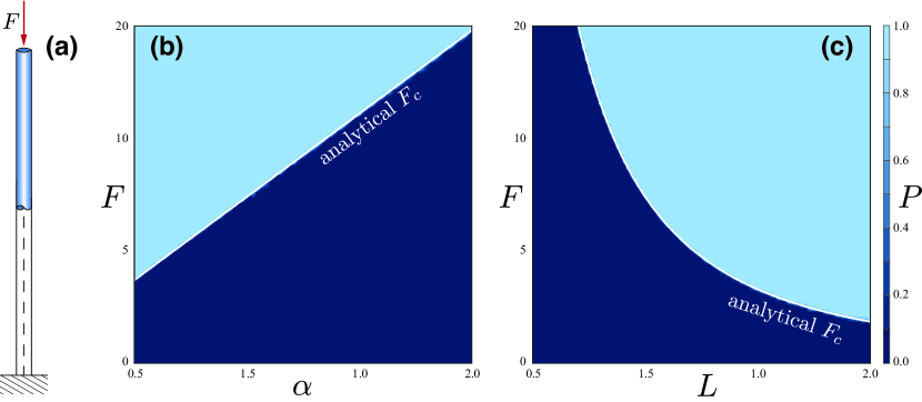
Refer to caption
Figure 13: Euler buckling instability. (a) Inextensible and unshearable rod vertically initialized and subject to the axial load F𝐹F. (b) Probability P𝑃P of observing an instability event as a function of the compression force F𝐹F and the bending rigidity α𝛼\alpha for a fixed length L=1𝐿1L=1 m. The corresponding analytical solution is overlaid as reference (white line). (c) Probability P𝑃P of observing an instability event as a function of the compression force F𝐹F and the length L𝐿L for a fixed bending rigidity α=1𝛼1\alpha=1 Nm2. The corresponding analytical solution is overlaid as reference (white line). The probability P𝑃P is determined by performing ten simulations for each pair of parameters (F,α)𝐹𝛼(F,\alpha) or (F,L)𝐹𝐿(F,L). Each simulation is initially perturbed by applying to every discretization node a small random force sampled from a uniform distribution, such that FR𝒰(0,102)similar-tonormsubscript𝐹𝑅𝒰0superscript102\|F_{R}\|\sim\mathcal{U}(0,10^{-2}) N. The occurrence of an instability is detected whenever the rod bending energy EB>Ethsubscript𝐸𝐵subscript𝐸𝑡E_{B}>E_{th} with Eth=103subscript𝐸𝑡superscript103E_{th}=10^{-3} J. Settings: rod’s mass mr=1subscript𝑚𝑟1m_{r}=1 kg, twist stiffness β=2α/3𝛽2𝛼3\beta=2\alpha/3 Nm2, shear/stretch matrix 𝐒=105𝟏𝐒superscript1051\mathbf{S}=10^{5}\cdot\boldsymbol{1} N, bend/twist matrix 𝐁=diag(α,α,β)𝐁diag𝛼𝛼𝛽\mathbf{B}=\text{diag}(\alpha,\alpha,\beta) Nm2, radius r=0.025L𝑟0.025𝐿r=0.025L m, discretization elements n=100𝑛100n=100 m-1, timestep δt=105𝛿𝑡superscript105\delta t=10^{-5} s, simulation time Tsim=10subscript𝑇sim10T_{\text{sim}}=10 s, dissipation constant γ=0𝛾0\gamma=0.

E.2 Mitchell buckling instability

The Euler buckling benchmark allows us to test the capability of our solver to capture the onset of an instability relative to the bending modes. Next we consider the Mitchell buckling instability that simultaneously accounts for both bend and twist. When the ends of an isotropic, inextensible and unshearable filament are joined together, the resulting configuration is a planar circular shape. If the two ends are twisted by a given angle and glued together, a circular shape with uniform twist density is obtained. When the total twist ΦΦ\Phi, i.e. the integrated twist line density along the filament, exceeds a critical value ΦcsubscriptΦ𝑐\Phi_{c} the rod buckles out of plane. This critical total twist can be expressed analytically Goriely:2006 as

Φc=23πβ/α,subscriptΦ𝑐23𝜋𝛽𝛼\Phi_{c}=\frac{2\sqrt{3}\pi}{\beta/\alpha}, (80)

where α𝛼\alpha and β𝛽\beta are, respectively, the bending and twist rigidities.

We explore the phase space F𝐹F-(β/α)𝛽𝛼(\beta/\alpha) and determine the probability of a randomly perturbed rod to undergo a buckling event, characterized by the translational energy exceeding a small threshold value ET>Ethsubscript𝐸𝑇subscript𝐸𝑡E_{T}>E_{th}. As can be seen in Fig. 14, our results show a sharp transition in agreement with the exact solution of Eq. (80).
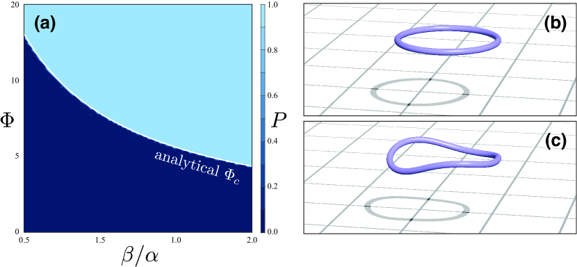
Refer to caption
Figure 14: Mitchell buckling instability. (a) Probability P𝑃P of observing an instability event as a function of the total twist ΦΦ\Phi and the ratio between bending and twist rigidities β/α𝛽𝛼\beta/\alpha. The corresponding analytical solution is overlaid as reference (white line). The probability P𝑃P is determined by performing ten simulations for each pair of parameters (Φ,β/α)Φ𝛽𝛼(\Phi,\beta/\alpha). Each simulation is initially perturbed by applying to every discretization node a small random force sampled from a uniform distribution, such that FR𝒰(0,103)similar-tonormsubscript𝐹𝑅𝒰0superscript103\|F_{R}\|\sim\mathcal{U}(0,10^{-3}) N. The occurrence of an instability is detected whenever the rod translational energy ET>Ethsubscript𝐸𝑇subscript𝐸𝑡E_{T}>E_{th} with Eth=104subscript𝐸𝑡superscript104E_{th}=10^{-4} J. (b-c) Visualization of a Mitchell bucking instability event for Φ=10Φ10\Phi=10 and β/α=2𝛽𝛼2\beta/\alpha=2. Settings: rod’s mass mr=1subscript𝑚𝑟1m_{r}=1 kg, length L=1𝐿1L=1 m, bending stiffness α=1𝛼1\alpha=1 Nm2, shear/stretch matrix 𝐒=105𝟏𝐒superscript1051\mathbf{S}=10^{5}\cdot\boldsymbol{1} N, bend/twist matrix 𝐁=diag(α,α,β)𝐁diag𝛼𝛼𝛽\mathbf{B}=\text{diag}(\alpha,\alpha,\beta) Nm2, radius r=0.01L𝑟0.01𝐿r=0.01L m, discretization elements n=50𝑛50n=50 m-1, timestep δt=105𝛿𝑡superscript105\delta t=10^{-5} s, simulation time Tsim=2subscript𝑇sim2T_{\text{sim}}=2 s, dissipation constant γ=0𝛾0\gamma=0.

E.3 Twist forced vibrations in a stretched rod

Next we examine the problem of twisting waves generated in a rod axially stretched, as illustrated in Fig. 15a. The coupling between stretching and the other dynamic modes tests the rescaling in terms of the dilatation factor e𝑒e of Eqs. (14, 15).

The rod is clamped at one end, stretched by the quantity ΔL=(e1)L^Δ𝐿𝑒1^𝐿\Delta L=(e-1)\hat{L}, and forced to angularly vibrate about the axial direction by applying at the free end the couple Avsin(2πfvt)subscript𝐴𝑣2𝜋subscript𝑓𝑣𝑡A_{v}\sin(2\pi f_{v}t), where Avsubscript𝐴𝑣A_{v} and fvsubscript𝑓𝑣f_{v} are the corresponding forcing amplitude and frequency. In the case of no internal dissipation and constant circular sections, the induced standing angular wave θ(s,t)𝜃𝑠𝑡\theta(s,t) can be determined analytically. The dynamics of twisting yields the wave equation for the angular displacement Selvadurai:2000

2θs2=1cs2θt2,superscript2𝜃superscript𝑠21subscript𝑐𝑠superscript2𝜃superscript𝑡2\frac{\partial^{2}\theta}{\partial s^{2}}=\frac{1}{c_{s}}\frac{\partial^{2}\theta}{\partial t^{2}}, (81)

where cs=G/ρsubscript𝑐𝑠𝐺𝜌c_{s}=\sqrt{G/\rho} is the shear wave velocity, G𝐺G is the shear modulus, and ρ𝜌\rho is the density. By assuming a solution of the form θ(s,t)=ϕ(s)sin(2πfvt)𝜃𝑠𝑡italic-ϕ𝑠2𝜋subscript𝑓𝑣𝑡\theta(s,t)=\phi(s)\sin(2\pi f_{v}t), and by applying the boundary conditions ϕ(0)=0italic-ϕ00\phi(0)=0 and dsϕ(0)=Cv/(I^3G)subscript𝑑𝑠italic-ϕ0subscript𝐶𝑣subscript^𝐼3𝐺d_{s}\phi(0)=C_{v}/(\hat{I}_{3}G) with Cvsubscript𝐶𝑣C_{v} twisting torque and I^3subscript^𝐼3\hat{I}_{3} second area moment of inertia about the axial direction, we can solve Eq. (81) obtaining

θ(s,t)=Avcs2πfvGI^3e2sin(2πfves^cs)cos(2πfveL^cs)sin(2πfvt).𝜃𝑠𝑡subscript𝐴𝑣subscript𝑐𝑠2𝜋subscript𝑓𝑣𝐺subscript^𝐼3superscript𝑒22𝜋subscript𝑓𝑣𝑒^𝑠subscript𝑐𝑠2𝜋subscript𝑓𝑣𝑒^𝐿subscript𝑐𝑠2𝜋subscript𝑓𝑣𝑡\theta(s,t)=\frac{A_{v}c_{s}}{2\pi f_{v}G\displaystyle\frac{\hat{I}_{3}}{e^{2}}}\cdot\frac{\sin\left(\displaystyle\frac{2\pi f_{v}e\hat{s}}{c_{s}}\right)}{\cos\left(\displaystyle\frac{2\pi f_{v}e\hat{L}}{c_{s}}\right)}\cdot\sin(2\pi f_{v}t). (82)

As can be seen in Fig. 15b, our numerical method recovers the derived analytical solution for the twist angular displacement along the stretched rod. Moreover, the solver consistently exhibits a second order convergence in time and space given the error metric ϵ=θθnitalic-ϵnorm𝜃superscript𝜃𝑛\epsilon=\|\theta-\theta^{n}\|, where θnsuperscript𝜃𝑛\theta^{n} represents our numerical solutions in the limit of refinement (Fig. 15c).
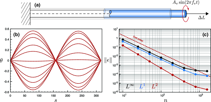
Refer to caption
Figure 15: Time-space convergence study for twist forced vibrations in a stretched rod. (a) We consider a rod clamped at one end, forced to vibrate by applying the periodic couple Avsin(2πfvt)subscript𝐴𝑣2𝜋subscript𝑓𝑣𝑡A_{v}\sin(2\pi f_{v}t) to the free end, and characterized by rest length L^^𝐿\hat{L} which is extended to a final length L=eL^𝐿𝑒^𝐿L=e\hat{L}. (b) Comparison between analytical θ𝜃\theta (black lines) and numerical θnsuperscript𝜃𝑛\theta^{n} (red dashed lines) angular displacement with respect to the reference configuration along a stretched rod. Each red (numerical simulation) and black (analytical solution) line corresponds to the angular displacement along a rod discretized with n=1600𝑛1600n=1600 elements, and sampled at regular intervals Δt=Tv/10Δ𝑡subscript𝑇𝑣10\Delta t=T_{v}/10 within one loading period Tv=fv1subscript𝑇𝑣superscriptsubscript𝑓𝑣1T_{v}=f_{v}^{-1}. (c) Norms L(ϵ)superscript𝐿italic-ϵL^{\infty}(\epsilon) (black), L1(ϵ)superscript𝐿1italic-ϵL^{1}(\epsilon) (blue) and L2(ϵ)superscript𝐿2italic-ϵL^{2}(\epsilon) (red) of the error ϵ=θθnitalic-ϵnorm𝜃superscript𝜃𝑛\epsilon=\|\theta-\theta^{n}\| at different levels of time-space resolution are plotted against the number of discretization elements n𝑛n. Here, the time discretization δt𝛿𝑡\delta t is slaved by the spatial discretization n𝑛n according to δt=104δl𝛿𝑡superscript104𝛿𝑙\delta t=10^{-4}\delta l seconds. For all studies, we used the following settings: rod’s density ρ=10𝜌10\rho=10 kg/m3, Young’s modulus E=106𝐸superscript106E=10^{6} Pa, shear modulus G=2E/3𝐺2𝐸3G=2E/3 Pa, shear/stretch matrix 𝐒^=diag(4GA^/3,4GA^/3,EA^)^𝐒diag4𝐺^𝐴34𝐺^𝐴3𝐸^𝐴\hat{\mathbf{S}}=\text{diag}(4G\hat{A}/3,4G\hat{A}/3,E\hat{A}) N, bend/twist matrix 𝐁^=diag(EI^1,EI^2,GI^3)^𝐁diag𝐸subscript^𝐼1𝐸subscript^𝐼2𝐺subscript^𝐼3\hat{\mathbf{B}}=\text{diag}(E\hat{I}_{1},E\hat{I}_{2},G\hat{I}_{3}) Nm2, forcing amplitude Av=103subscript𝐴𝑣superscript103A_{v}=10^{3} Nm, forcing frequency fv=1subscript𝑓𝑣1f_{v}=1 s-1, dilatation factor e𝑒e=1.051.051.05, rest length L^^𝐿\hat{L}=E/ρ/(efv)𝐸𝜌𝑒subscript𝑓𝑣\sqrt{E/\rho}/(ef_{v}) m, rest radius r^^𝑟\hat{r}=0.50.50.5 m, simulation time Tsimsubscript𝑇simT_{\text{sim}}=200020002000 s. We enabled dissipation in the early stages of the simulations, letting γ𝛾\gamma decay exponentially in time to a zero value.

Appendix F Further friction validations

F.1 Validation of rolling friction model

Here we validate the friction model introduced in Section IV.0.5 on three test cases that can be analytically characterized. In all benchmarks we consider a rigid, unshearable, inextensible straight rod of mass m𝑚m, length L𝐿L, radius r𝑟r, axial mass second moment of inertia J𝐽J. The rod interacts with a surface characterized by static and kinetic friction coefficients μssubscript𝜇𝑠\mu_{s} and μksubscript𝜇𝑘\mu_{k}, thus assuming isotropic friction.

Refer to caption
Figure 16: Rolling static and dynamic friction. (a) A rod initially at rest on a plane inclined of the angle αssubscript𝛼𝑠\alpha_{s}, rolls or slips down with linear and angular velocities v𝑣v and ω𝜔\omega due to its own weight mg𝑚𝑔mg. (b) Translational ET=mv2/2subscript𝐸𝑇𝑚superscript𝑣22E_{T}=mv^{2}/2 (analytical solution - black line, numerical solution - blue line) and rotational ER=Jω2/2subscript𝐸𝑅𝐽superscript𝜔22E_{R}=J\omega^{2}/2 (analytical solution - dashed black line, numerical solution - orange line) energies are plotted against the angle αssubscript𝛼𝑠\alpha_{s}. Settings: length L=1𝐿1L=1 m, radius r=0.025𝑟0.025r=0.025 m, mass m=1𝑚1m=1 kg, Young’s modulus E=109𝐸superscript109E=10^{9} Pa, shear modulus G=2E/3𝐺2𝐸3G=2E/3 Pa, shear/stretch matrix 𝐒=104𝟏𝐒superscript1041\mathbf{S}=10^{4}\cdot\boldsymbol{1} N, bend/twist matrix 𝐁=diag(EI1,EI2,GI3)𝐁diag𝐸subscript𝐼1𝐸subscript𝐼2𝐺subscript𝐼3\mathbf{B}=\text{diag}(EI_{1},EI_{2},GI_{3}) Nm2, dissipation constant γ=106𝛾superscript106\gamma=10^{-6} kg/(ms), gravity g=9.81𝑔9.81g=9.81 m/s2, static and kinetic friction coefficients μs=0.4subscript𝜇𝑠0.4\mu_{s}=0.4 and μk=0.2subscript𝜇𝑘0.2\mu_{k}=0.2, friction threshold velocity vϵ=104subscript𝑣italic-ϵsuperscript104v_{\epsilon}=10^{-4} m/s, ground stiffness and viscous dissipation kw=10subscript𝑘𝑤10k_{w}=10 kg/s2 and γw=104subscript𝛾𝑤superscript104\gamma_{w}=10^{-4} kg/s, discretization elements n=50𝑛50n=50, timestep δt=106𝛿𝑡superscript106\delta t=10^{-6} s, simulation time T=0.5𝑇0.5T=0.5 s. (c) Rod set in motion by the external couple Cssubscript𝐶𝑠C_{s} on a horizontal plane. (d) Translational ETsubscript𝐸𝑇E_{T} and rotational ERsubscript𝐸𝑅E_{R} energies are plotted agains the couple Cssubscript𝐶𝑠C_{s}. Color scheme and settings identical to those of panel (b) except for the simulation time T=1𝑇1T=1 s. (e) Rod with initial velocity Vssubscript𝑉𝑠V_{s} slows down due to kinetic friction until the no slip condition is reached. (f) Translational ETsubscript𝐸𝑇E_{T} and rotational ERsubscript𝐸𝑅E_{R} energies are plotted agains the relative mass moment of inertia ratio λ/2𝜆2\lambda/2. Color scheme and settings identical to those of panel (b) except for the simulation time T=2𝑇2T=2 s, and the friction threshold velocity vϵ=106subscript𝑣italic-ϵsuperscript106v_{\epsilon}=10^{-6} m/s.

In the first test the rod is initially at rest on a plane inclined of the angle αssubscript𝛼𝑠\alpha_{s}, as depicted in Fig. 16a. Due to the gravitational acceleration g𝑔g the rod starts rolling or slipping, depending on αssubscript𝛼𝑠\alpha_{s}, down the plane. The linear v𝑣v and angular ω𝜔\omega velocities of the filament, and therefore the corresponding translational ET=mv2/2subscript𝐸𝑇𝑚superscript𝑣22E_{T}=mv^{2}/2 and rotational ER=Jω2/2subscript𝐸𝑅𝐽superscript𝜔22E_{R}=J\omega^{2}/2 energies can be analytically determined.

By recalling Eq. (42), the force necessary to ensure rolling without slip takes the form Fnoslip=F/3=mgsin(αs)/3subscript𝐹noslipsubscript𝐹parallel-to3𝑚𝑔subscript𝛼𝑠3F_{\text{noslip}}=-F_{\parallel}/3=-mg\sin(\alpha_{s})/3. Given the maximum static friction force Fs=μsF=μsmgcos(αs)subscript𝐹𝑠subscript𝜇𝑠subscript𝐹perpendicular-tosubscript𝜇𝑠𝑚𝑔subscript𝛼𝑠F_{s}=\mu_{s}F_{\perp}=\mu_{s}mg\cos(\alpha_{s}) in the case |Fnoslip||Fs|subscript𝐹noslipsubscript𝐹𝑠|F_{\text{noslip}}|\leq|F_{s}| we have a=(F+Fnoslip)/m𝑎subscript𝐹parallel-tosubscript𝐹noslip𝑚a=(F_{\parallel}+F_{\text{noslip}})/m. Therefore, at the time T𝑇T after releasing the rod, linear and angular velocities read, respectively, v=aT𝑣𝑎𝑇v=aT and ω=ω˙T=(a/r)T𝜔˙𝜔𝑇𝑎𝑟𝑇\omega=\dot{\omega}T=(a/r)T expressing the no slip kinematic constraint between linear a𝑎a and angular ω˙˙𝜔\dot{\omega} accelerations. On the contrary, if |Fnoslip|>|Fs|subscript𝐹noslipsubscript𝐹𝑠|F_{\text{noslip}}|>|F_{s}| the rod starts slipping and linear and angular accelerations are no longer coupled, so that after the time T𝑇T we have a=(FμkF)/m𝑎subscript𝐹parallel-tosubscript𝜇𝑘subscript𝐹perpendicular-to𝑚a=(F_{\parallel}-\mu_{k}F_{\perp})/m, v=aT𝑣𝑎𝑇v=aT, ω=ω˙T=(μkFr/J)T𝜔˙𝜔𝑇subscript𝜇𝑘subscript𝐹perpendicular-to𝑟𝐽𝑇\omega=\dot{\omega}T=(\mu_{k}F_{\perp}r/J)T. Therefore, translational and rotational energies as a function of αssubscript𝛼𝑠\alpha_{s} finally read

ET={2mg2T2sin2(αs)9if |Fnoslip||Fs|mg2T2[sin(αs)μkcos(αs)]22if |Fnoslip|>|Fs|subscript𝐸𝑇cases2𝑚superscript𝑔2superscript𝑇2superscript2subscript𝛼𝑠9if subscript𝐹noslipsubscript𝐹𝑠𝑚superscript𝑔2superscript𝑇2superscriptdelimited-[]subscript𝛼𝑠subscript𝜇𝑘subscript𝛼𝑠22if subscript𝐹noslipsubscript𝐹𝑠E_{T}=\begin{dcases}\frac{2mg^{2}T^{2}\sin^{2}(\alpha_{s})}{9}&\text{if }|F_{\text{noslip}}|\leq|F_{s}|\\ \frac{mg^{2}T^{2}\left[\sin(\alpha_{s})-\mu_{k}\cos(\alpha_{s})\right]^{2}}{2}&\text{if }|F_{\text{noslip}}|>|F_{s}|\end{dcases}

and

ER={2Jg2T2sin2(αs)9r2if |Fnoslip||Fs|μk2m2g2r2T2cos2(αs)2Jif |Fnoslip|>|Fs|subscript𝐸𝑅cases2𝐽superscript𝑔2superscript𝑇2superscript2subscript𝛼𝑠9superscript𝑟2if subscript𝐹noslipsubscript𝐹𝑠superscriptsubscript𝜇𝑘2superscript𝑚2superscript𝑔2superscript𝑟2superscript𝑇2superscript2subscript𝛼𝑠2𝐽if subscript𝐹noslipsubscript𝐹𝑠E_{R}=\begin{dcases}\frac{2Jg^{2}T^{2}\sin^{2}(\alpha_{s})}{9r^{2}}&\text{if }|F_{\text{noslip}}|\leq|F_{s}|\\ \frac{\mu_{k}^{2}m^{2}g^{2}r^{2}T^{2}\cos^{2}(\alpha_{s})}{2J}&\text{if }|F_{\text{noslip}}|>|F_{s}|\end{dcases}

As can be noticed in Fig. 16b, our numerical approach faithfully reproduces the derived analytical solution, accurately capturing the discontinuity at the transition between pure rolling and slipping.

The second test case of Fig. 16c,d entails a rod set in motion by the external couple Cssubscript𝐶𝑠C_{s} on a horizontal plane. Depending on the magnitude of the load the filament exhibits pure rolling or slipping motion. By recalling Eq. (42), the force necessary to ensure rolling without slip takes the form Fnoslip=2Cs/(3r)subscript𝐹noslip2subscript𝐶𝑠3𝑟F_{\text{noslip}}=2C_{s}/(3r). Given the maximum static friction force Fs=μsF=μsmgsubscript𝐹𝑠subscript𝜇𝑠subscript𝐹perpendicular-tosubscript𝜇𝑠𝑚𝑔F_{s}=\mu_{s}F_{\perp}=\mu_{s}mg in the case |Fnoslip||Fs|subscript𝐹noslipsubscript𝐹𝑠|F_{\text{noslip}}|\leq|F_{s}| we have a=Fnoslip/m𝑎subscript𝐹noslip𝑚a=F_{\text{noslip}}/m. Therefore, at the time T𝑇T after releasing the rod, linear and angular velocities read, respectively, v=aT𝑣𝑎𝑇v=aT and ω=ω˙T=(a/r)T𝜔˙𝜔𝑇𝑎𝑟𝑇\omega=\dot{\omega}T=(a/r)T expressing the no slip kinematic constraint between linear a𝑎a and angular ω˙˙𝜔\dot{\omega} accelerations. On the contrary, if |Fnoslip|>|Fs|subscript𝐹noslipsubscript𝐹𝑠|F_{\text{noslip}}|>|F_{s}| the rod starts slipping and linear and angular accelerations are no longer coupled, so that after the time T𝑇T we have a=μkF/m𝑎subscript𝜇𝑘subscript𝐹perpendicular-to𝑚a=\mu_{k}F_{\perp}/m, v=aT𝑣𝑎𝑇v=aT, ω=ω˙T=J1(CsμkFr)T𝜔˙𝜔𝑇superscript𝐽1subscript𝐶𝑠subscript𝜇𝑘subscript𝐹perpendicular-to𝑟𝑇\omega=\dot{\omega}T=J^{-1}(C_{s}-\mu_{k}F_{\perp}r)T. Therefore, translational and rotational energies as a function of Cssubscript𝐶𝑠C_{s} finally read

ET={2T2Cs29mr2if |Fnoslip||Fs|mμk2g2T22if |Fnoslip|>|Fs|subscript𝐸𝑇cases2superscript𝑇2superscriptsubscript𝐶𝑠29𝑚superscript𝑟2if subscript𝐹noslipsubscript𝐹𝑠𝑚superscriptsubscript𝜇𝑘2superscript𝑔2superscript𝑇22if subscript𝐹noslipsubscript𝐹𝑠E_{T}=\begin{dcases}\frac{2T^{2}C_{s}^{2}}{9mr^{2}}&\text{if }|F_{\text{noslip}}|\leq|F_{s}|\\ \frac{m\mu_{k}^{2}g^{2}T^{2}}{2}&\text{if }|F_{\text{noslip}}|>|F_{s}|\end{dcases}

and

ER={2JT2Cs29r4m2if |Fnoslip||Fs|(Csμkmgr)2T22Jif |Fnoslip|>|Fs|subscript𝐸𝑅cases2𝐽superscript𝑇2superscriptsubscript𝐶𝑠29superscript𝑟4superscript𝑚2if subscript𝐹noslipsubscript𝐹𝑠superscriptsubscript𝐶𝑠subscript𝜇𝑘𝑚𝑔𝑟2superscript𝑇22𝐽if subscript𝐹noslipsubscript𝐹𝑠E_{R}=\begin{dcases}\frac{2JT^{2}C_{s}^{2}}{9r^{4}m^{2}}&\text{if }|F_{\text{noslip}}|\leq|F_{s}|\\ \frac{(C_{s}-\mu_{k}mgr)^{2}T^{2}}{2J}&\text{if }|F_{\text{noslip}}|>|F_{s}|\end{dcases}

As can be noticed in Fig. 16d, again our numerical approach faithfully reproduces the derived analytical solution, accurately capturing the discontinuity at the transition between pure rolling and slipping.

In the last test case we consider a rod of initial velocity Vssubscript𝑉𝑠V_{s} in the direction parallel to a horizontal plane and perpendicular to the filament axis (Fig. 16e), and we vary the relative mass moment of inertia ratio λ=2J/(mr2)𝜆2𝐽𝑚superscript𝑟2\lambda=2J/(mr^{2}). Initially the rod slips on the surface and gradually slows down, due to the effect of the kinetic friction, to a point for which linear a𝑎a and angular velocity ω𝜔\omega meet the kinematic constraint veq=rωeqsubscript𝑣𝑒𝑞𝑟subscript𝜔𝑒𝑞v_{eq}=r\omega_{eq} characteristic of pure rolling motion. The frictional force F𝐹F induces the torque M=rF𝑀𝑟𝐹M=rF, so that over a period of time T𝑇T we have v=VsFT/m𝑣subscript𝑉𝑠𝐹𝑇𝑚v=V_{s}-FT/m and ω=rFT/J𝜔𝑟𝐹𝑇𝐽\omega=rFT/J. By enforcing the no slip kinematic constraint VsFT/m=r2FT/Jsubscript𝑉𝑠𝐹𝑇𝑚superscript𝑟2𝐹𝑇𝐽V_{s}-FT/m=r^{2}FT/J, we have that FT=Vs/(r2/J+1/m)𝐹𝑇subscript𝑉𝑠superscript𝑟2𝐽1𝑚FT=V_{s}/(r^{2}/J+1/m). This allows us to directly compute veqsubscript𝑣𝑒𝑞v_{eq} and ωeqsubscript𝜔𝑒𝑞\omega_{eq} and the corresponding translational and rotational energies, yielding

ETeq=mVs221(1+λ/2)2,EReq=mVs22λ/2(1+λ/2)2.formulae-sequencesubscriptsuperscript𝐸𝑒𝑞𝑇𝑚superscriptsubscript𝑉𝑠221superscript1𝜆22subscriptsuperscript𝐸𝑒𝑞𝑅𝑚superscriptsubscript𝑉𝑠22𝜆2superscript1𝜆22E^{eq}_{T}=\frac{mV_{s}^{2}}{2}\frac{1}{(1+\lambda/2)^{2}},~{}~{}~{}~{}~{}~{}~{}E^{eq}_{R}=\frac{mV_{s}^{2}}{2}\frac{\lambda/2}{(1+\lambda/2)^{2}}. (83)

As depicted in Fig. 16f, our numerical approach accurately reproduces the predicted energies as a function of λ𝜆\lambda.

F.2 Validation of anisotropic longitudinal friction model

After validating our rolling friction model, we turn to its longitudinal counterpart. Here we consider a straight, rigid, inextensible and unshearable rod which is axially pulled or pushed with force 𝐅𝐅\mathbf{F} for a fixed period of time T𝑇T (Fig. 17). Anisotrpy is captured through the forward μsfsuperscriptsubscript𝜇𝑠𝑓\mu_{s}^{f}, μkfsuperscriptsubscript𝜇𝑘𝑓\mu_{k}^{f} and backward μsbsuperscriptsubscript𝜇𝑠𝑏\mu_{s}^{b}, μkbsuperscriptsubscript𝜇𝑘𝑏\mu_{k}^{b} static and kinetic coefficients. For 𝐅𝐭0𝐅𝐭0\mathbf{F}\cdot\mathbf{t}\geq 0 the rod translational energy takes the form

ETf={0if |𝐅||μsfmg|T22m(|𝐅|μkfmg)2if |𝐅|>|μsfmg|,subscriptsuperscript𝐸𝑓𝑇cases0if 𝐅subscriptsuperscript𝜇𝑓𝑠𝑚𝑔superscript𝑇22𝑚superscript𝐅superscriptsubscript𝜇𝑘𝑓𝑚𝑔2if 𝐅subscriptsuperscript𝜇𝑓𝑠𝑚𝑔E^{f}_{T}=\begin{dcases}0&\text{if }|\mathbf{F}|\leq|\mu^{f}_{s}mg|\\ \frac{T^{2}}{2m}(|\mathbf{F}|-\mu_{k}^{f}mg)^{2}&\text{if }|\mathbf{F}|>|\mu^{f}_{s}mg|\end{dcases},

while for 𝐅𝐭<0𝐅𝐭0\mathbf{F}\cdot\mathbf{t}<0 we have

ETb={0if |𝐅||μsbmg|T22m(|𝐅|μkbmg)2if |𝐅|>|μsbmg|.subscriptsuperscript𝐸𝑏𝑇cases0if 𝐅subscriptsuperscript𝜇𝑏𝑠𝑚𝑔superscript𝑇22𝑚superscript𝐅superscriptsubscript𝜇𝑘𝑏𝑚𝑔2if 𝐅subscriptsuperscript𝜇𝑏𝑠𝑚𝑔E^{b}_{T}=\begin{dcases}0&\text{if }|\mathbf{F}|\leq|\mu^{b}_{s}mg|\\ \frac{T^{2}}{2m}(|\mathbf{F}|-\mu_{k}^{b}mg)^{2}&\text{if }|\mathbf{F}|>|\mu^{b}_{s}mg|\end{dcases}.

As can be seen in Fig. 17, our numerical method reproduces the above theoretical predictions.
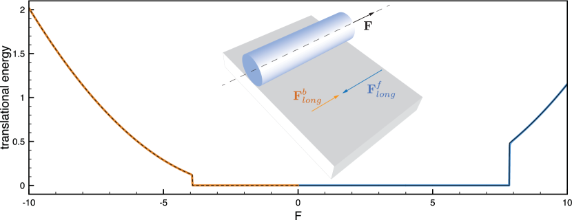
Refer to caption
Figure 17: Anisotropic static and kinetic longitudinal friction. A rod initially at rest on a horizontal plane is pulled longitudinally with force 𝐅𝐅\mathbf{F}. The system is characterized by anisotropic friction so that resistance forces in the forward direction 𝐅longfsubscriptsuperscript𝐅𝑓𝑙𝑜𝑛𝑔\mathbf{F}^{f}_{long} are larger than in the backward direction 𝐅longbsubscriptsuperscript𝐅𝑏𝑙𝑜𝑛𝑔\mathbf{F}^{b}_{long}. The plot illustrates the behavior of the total rod’s translational energy ETsubscript𝐸𝑇E_{T} as a function of the force 𝐅𝐅\mathbf{F} applied. Blue and solid black lines correspond to, respectively, simulated and analytical ETsubscript𝐸𝑇E_{T} for a rod pulled forward. Orange and dashed black lines correspond to, respectively, simulated and analytical ETsubscript𝐸𝑇E_{T} for a rod pulled backward. Settings: length L=1𝐿1L=1 m, radius r=0.025𝑟0.025r=0.025 m, mass m=1𝑚1m=1 kg, Young’s modulus E=105𝐸superscript105E=10^{5} Pa, shear modulus G=2E/3𝐺2𝐸3G=2E/3 Pa, shear/stretch matrix 𝐒=104𝟏𝐒superscript1041\mathbf{S}=10^{4}\cdot\boldsymbol{1} N, bend/twist matrix 𝐁=diag(EI1,EI2,GI3)𝐁diag𝐸subscript𝐼1𝐸subscript𝐼2𝐺subscript𝐼3\mathbf{B}=\text{diag}(EI_{1},EI_{2},GI_{3}) Nm2, dissipation constant γ=106𝛾superscript106\gamma=10^{-6} kg/(ms), gravity g=9.81𝑔9.81g=9.81 m/s2, static and kinetic forward friction coefficients μsf=0.8subscriptsuperscript𝜇𝑓𝑠0.8\mu^{f}_{s}=0.8 and μkf=0.4subscriptsuperscript𝜇𝑓𝑘0.4\mu^{f}_{k}=0.4, static and kinetic backward friction coefficients μsb=0.4subscriptsuperscript𝜇𝑏𝑠0.4\mu^{b}_{s}=0.4 and μkb=0.2subscriptsuperscript𝜇𝑏𝑘0.2\mu^{b}_{k}=0.2, friction threshold velocity vϵ=104subscript𝑣italic-ϵsuperscript104v_{\epsilon}=10^{-4} m/s, ground stiffness and viscous dissipation kw=10subscript𝑘𝑤10k_{w}=10 kg/s2 and γw=104subscript𝛾𝑤superscript104\gamma_{w}=10^{-4} kg/s, discretization elements n=50𝑛50n=50, timestep δt=105𝛿𝑡superscript105\delta t=10^{-5} s, simulation time T=0.25𝑇0.25T=0.25 s.

F.3 Isotropic vs. anisotropic friction driven locomotion

In this section we illustrate the effect of symmetry breaking via anisotropic friction in a system constituted by a soft filament interacting via surface friction with a solid substrate. If we consider isotropic friction and a specular muscular activation pattern by setting the control values β1=β4subscript𝛽1subscript𝛽4\beta_{1}=\beta_{4} and β2=β3subscript𝛽2subscript𝛽3\beta_{2}=\beta_{3} and the wave number 2π/λm=02𝜋subscript𝜆𝑚02\pi/\lambda_{m}=0 (see Section IV.0.2), then the system is symmetric (up to inertial effects that can be neglected for small Froude numbers). Therefore, over any activation cycle the snake center of mass does not move. On the contrary, if we introduce anisotropy the snake will be able to slowly move (the capability to effectively move is impaired by the absence of the traveling gait component since 2π/λm=02𝜋subscript𝜆𝑚02\pi/\lambda_{m}=0).

As can be observed in Fig. 18, this prediction is captured by our numerical scheme, which accurately resolves the physical mechanisms at play. Moreover, this test shows once again how our methodology is robust in terms of numerical noise as no spurious displacements or rotations are generated in the symmetric case (Fig. 18a,b).
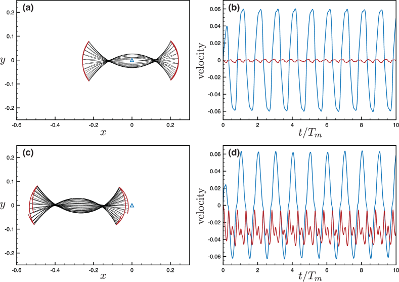
Refer to caption
Figure 18: Isotropic vs. anisotropic friction driven locomotion. (a) Gait envelope computed over the 10th muscular activation cycle in the case of isotropic friction. The blue triangle denotes the location of the snake’s center of mass at time t=0𝑡0t=0, reported as reference. (b) Lateral (blue) and forward (red) velocities as functions of time normalized by the activation period Tmsubscript𝑇𝑚T_{m} in the case of isotropic friction. (c) Gait envelope computed over the 10th muscular activation cycle in the case of anisotropic friction. The blue triangle denotes the location of the snake’s center of mass at time t=0𝑡0t=0, reported as reference. (d) Lateral (blue) and forward (red) velocities as functions of time normalized by the activation period Tmsubscript𝑇𝑚T_{m} in the case of anisotropic friction. Settings: length L=0.5𝐿0.5L=0.5 m, radius r=0.025𝑟0.025r=0.025 m, mass m=1𝑚1m=1 kg, Young’s modulus E=107𝐸superscript107E=10^{7} Pa, shear modulus G=2E/3𝐺2𝐸3G=2E/3 Pa, shear/stretch matrix 𝐒=105𝟏𝐒superscript1051\mathbf{S}=10^{5}\cdot\boldsymbol{1} N, bend/twist matrix 𝐁=diag(EI1,EI2,GI3)𝐁diag𝐸subscript𝐼1𝐸subscript𝐼2𝐺subscript𝐼3\mathbf{B}=\text{diag}(EI_{1},EI_{2},GI_{3}) Nm2, dissipation constant γ=101𝛾superscript101\gamma=10^{-1} kg/(ms), gravity g=9.81𝑔9.81g=9.81 m/s2, static μsf=0.2subscriptsuperscript𝜇𝑓𝑠0.2\mu^{f}_{s}=0.2, μsr=μsfsubscriptsuperscript𝜇𝑟𝑠subscriptsuperscript𝜇𝑓𝑠\mu^{r}_{s}=\mu^{f}_{s}, μsb=μsfsubscriptsuperscript𝜇𝑏𝑠subscriptsuperscript𝜇𝑓𝑠\mu^{b}_{s}=\mu^{f}_{s} and kinetic μkf=0.1subscriptsuperscript𝜇𝑓𝑘0.1\mu^{f}_{k}=0.1, μkr=μkfsubscriptsuperscript𝜇𝑟𝑘subscriptsuperscript𝜇𝑓𝑘\mu^{r}_{k}=\mu^{f}_{k}, μkb=μkfsubscriptsuperscript𝜇𝑏𝑘subscriptsuperscript𝜇𝑓𝑘\mu^{b}_{k}=\mu^{f}_{k} friction coefficients in the isotropic case, static μsf=0.2subscriptsuperscript𝜇𝑓𝑠0.2\mu^{f}_{s}=0.2, μsr=2μsfsubscriptsuperscript𝜇𝑟𝑠2subscriptsuperscript𝜇𝑓𝑠\mu^{r}_{s}=2\mu^{f}_{s}, μsb=20μsfsubscriptsuperscript𝜇𝑏𝑠20subscriptsuperscript𝜇𝑓𝑠\mu^{b}_{s}=20\mu^{f}_{s} and kinetic μkf=0.1subscriptsuperscript𝜇𝑓𝑘0.1\mu^{f}_{k}=0.1, μkr=2μkfsubscriptsuperscript𝜇𝑟𝑘2subscriptsuperscript𝜇𝑓𝑘\mu^{r}_{k}=2\mu^{f}_{k}, μkb=20μkfsubscriptsuperscript𝜇𝑏𝑘20subscriptsuperscript𝜇𝑓𝑘\mu^{b}_{k}=20\mu^{f}_{k} friction coefficients in the anisotropic case, friction threshold velocity vϵ=108subscript𝑣italic-ϵsuperscript108v_{\epsilon}=10^{-8} m/s, ground stiffness and viscous dissipation kw=1subscript𝑘𝑤1k_{w}=1 kg/s2 and γw=106subscript𝛾𝑤superscript106\gamma_{w}=10^{-6} kg/s, discretization elements n=100𝑛100n=100, timestep δt=105𝛿𝑡superscript105\delta t=10^{-5} s, muscular activation period Tm=1subscript𝑇𝑚1T_{m}=1 s, wavelength λm=subscript𝜆𝑚\lambda_{m}=\infty, phase shift ϕm=0subscriptitalic-ϕ𝑚0\phi_{m}=0, torque B-spline coefficients βi=0,,5={0,10,15,15,10,0}subscript𝛽𝑖050101515100\beta_{i=0,\dots,5}=\{0,10,15,15,10,0\} Nm.

References

  • [1] G. Kirchhoff. Ueber das gleichgewicht und die bewegung eines unendlich dünnen elastischen stabes. Journal für die reine und angewandte Mathematik, 56:285–313, 1859.
  • [2] A. Clebsch. Théorie de l’élasticité des corps solides. Dunod, 1883.
  • [3] A.E.H. Love. A treatise on the mathematical theory of elasticity. Cambridge University Press, 1906.
  • [4] E. Cosserat and F. Cosserat. Théorie des corps déformables. Paris, 1909.
  • [5] S.S. Antman. The theory of rods. In Linear Theories of Elasticity and Thermoelasticity, pages 641–703. Springer, 1973.
  • [6] D.E. Harold. Kirchhoff’s theory of rods. Archive for History of Exact Sciences, 44(1):1–23, 1992.
  • [7] J. Langer and D.A. Singer. Lagrangian aspects of the kirchhoff elastic rod. SIAM review, 38(4):605–618, 1996.
  • [8] G.H.M. van der Heijden and J.M.T. Thompson. Helical and localised buckling in twisted rods: a unified analysis of the symmetric case. Nonlinear Dynamics, 21(1):71–99, 2000.
  • [9] V.G.A. Goss, G.H.M. Van der Heijden, J.M.T. Thompson, and S. Neukirch. Experiments on snap buckling, hysteresis and loop formation in twisted rods. Experimental mechanics, 45(2):101–111, 2005.
  • [10] G.A. Maugin and A.V. Metrikine. Mechanics of generalized continua. Advances in mechanics and mathematics, 21, 2010.
  • [11] V.G.A. Goss. The history of the planar elastica: insights into mechanics and scientific method. Science and Education, 18(8):1057–1082, 2009.
  • [12] Y. Yang, I. Tobias, and W.K. Olson. Finite element analysis of dna supercoiling. The Journal of chemical physics, 98(2):1673–1686, 1993.
  • [13] J. Spillmann and M. Teschner. Corde: Cosserat rod elements for the dynamic simulation of one-dimensional elastic objects. ACM Transactions on Graphics (TOG), pages 63–72, 2007.
  • [14] M. Bergou, M. Wardetzky, S. Robinson, B. Audoly, and E. Grinspun. Discrete elastic rods. ACM Transactions on Graphics (TOG), 27(3):1–12, 2008.
  • [15] W. Arne, N. Marheineke, A. Meister, and R. Wegener. Numerical analysis of cosserat rod and string models for viscous jets in rotational spinning processes. Mathematical Models and Methods in Applied Sciences, 20(10):1941–1965, 2010.
  • [16] B. Audoly, N. Clauvelin, P.T. Brun, M. Bergou, E. Grinspun, and M. Wardetzky. A discrete geometric approach for simulating the dynamics of thin viscous threads. Journal of Computational Physics, 253:18–49, 2013.
  • [17] C.W. Wolgemuth, T.R. Powers, and R.E. Goldstein. Twirling and whirling: Viscous dynamics of rotating elastic filaments. Physical Review Letters, 84(7):1623, 2000.
  • [18] M. Bergou, B. Audoly, E. Vouga, M. Wardetzky, and E. Grinspun. Discrete viscous threads. ACM Transactions on Graphics (TOG), 29(4):116, 2010.
  • [19] P.T. Brun, B. Audoly, N.M. Ribe, T.S. Eaves, and J.R. Lister. Liquid ropes: a geometrical model for thin viscous jet instabilities. Physical review letters, 114(17):174501, 2015.
  • [20] A. Goriely and M. Tabor. Spontaneous helix hand reversal and tendril perversion in climbing plants. Physical Review Letters, 80(7):1564, 1998.
  • [21] S.J. Gerbode, J.R. Puzey, A.G. McCormick, and L. Mahadevan. How the cucumber tendril coils and overwinds. Science, 337(6098):1087–1091, 2012.
  • [22] J.M. Kaldor, D.L. James, and S. Marschner. Simulating knitted cloth at the yarn level. ACM Transactions on Graphics (TOG), 27(3):65, 2008.
  • [23] K. Ward, F. Bertails, T.Y. Kim, S.R. Marschner, M.P. Cani, and M.C. Lin. A survey on hair modeling: Styling, simulation, and rendering. Visualization and Computer Graphics, IEEE Transactions on, 13(2):213–234, 2007.
  • [24] S. Kim, C. Laschi, and B. Trimmer. Soft robotics: a bioinspired evolution in robotics. Trends in biotechnology, 31(5):287–294, 2013.
  • [25] C.S. Haines, M.D. Lima, N. Li, G.M. Spinks, J. Foroughi, J.D. W. Madden, S.H. Kim, S. Fang, M. Jung de Andrade, F. Goktepe, O. Goktepe, S.M. Mirvakili, S. Naficy, X. Lepró, J. Oh, M.E. Kozlov, S.J. Kim, X. Xu, B.J. Swedlove, G.G. Wallace, and R.H. Baughman. Artificial muscles from fishing line and sewing thread. Science, 343(6173):868–872, 2014.
  • [26] S.J. Park, M. Gazzola, K.S. Park, S. Park, V. Di Santo, E.L. Blevins, J.U. Lind, P.H. Campbell, S. Dauth, A.K. Capulli, F.S. Pasqualini, S. Ahn, A. Cho, H. Yuan, B.M. Maoz, R. Vijaykumar, J.W. Choi, K. Deisseroth, G.V. Lauder, L. Mahadevan, and K.K. Parker. Phototactic guidance of a tissue-engineered soft-robotic ray. Science, 353(6295):158–162, 2016.
  • [27] J.M. Gere and S.P. Timoshenko. Mechanics of materials. Brooks/Cole, Pacific Grove, CA, 2001.
  • [28] L.D. Landau, J.S. Bell, M.J. Kearsley, L.P. Pitaevskii, E.M. Lifshitz, and J.B. Sykes. Electrodynamics of continuous media, volume 8. elsevier, 1984.
  • [29] J. Baillieul and M. Levi. Rotational elastic dynamics. Physica D: Nonlinear Phenomena, 27(1):43–62, 1987.
  • [30] M. Levi. Composition of rotations and parallel transport. Nonlinearity, 9(2):413, 1996.
  • [31] A. Goriely and M. Tabor. The nonlinear dynamics of filaments. Nonlinear Dynamics, 21(1):101–133, 2000.
  • [32] Olinde Rodrigues. Des lois géométriques qui régissent les déplacements d’un système solide dans l’espace: et de la variation des cordonnées provenant de ces déplacements considérés indépendamment des causes qui peuvent les produire. Journal de Mathématique Pures et Appliquées, 5:380–440, 1840.
  • [33] G. Sobottka, T. Lay, and A. Weber. Stable integration of the dynamic cosserat equations with application to hair modeling. Journal of WSCG, 2008.
  • [34] E. Grinspun, M. Desbrun, K. Polthier, P. Schroder, and A. Stern. Discrete differential geometry: an applied introduction. SIGGRAPH Course, 7, 2006.
  • [35] A. Kol, Brian B. Laird, and B.J. Leimkuhler. A symplectic method for rigid-body molecular simulation. The Journal of chemical physics, 107(7):2580–2588, 1997.
  • [36] J. Coyne. Analysis of the formation and elimination of loops in twisted cable. IEEE Journal of Oceanic Engineering, 15(2):72–83, 1990.
  • [37] S. Neukirch, G.H.M. van der Heijden, and J.M.T. Thompson. Writhing instabilities of twisted rods: from infinite to finite length. Journal of the Mechanics and Physics of Solids, 50(6):1175–1191, 2002.
  • [38] G.H.M. van der Heijden, S. Neukirch, V.G.A. Goss, and J.M.T. Thompson. Instability and self-contact phenomena in the writhing of clamped rods. International Journal of Mechanical Sciences, 45(1):161–196, 2003.
  • [39] E.E. Galloni and M. Kohen. Influence of the mass of the spring on its static and dynamic effects. American Journal of Physics, 47(12):1076–1078, 1979.
  • [40] Singiresu S Rao and Fook Fah Yap. Mechanical vibrations, volume 4. Addison-Wesley Reading, 1995.
  • [41] B.J. Torby. Advanced dynamics for engineers. Holt Rinehart and Winston, 1984.
  • [42] J.D. Altringham, John D., and I.A. Johnston. Modelling muscle power output in a swimming fish. Journal of Experimental Biology, 148(1):395–402, 1990.
  • [43] M. Gazzola, M. Argentina, and L. Mahadevan. Gait and speed selection in slender inertial swimmers. Proceedings of the National Academy of Sciences, 112(13):3874–3879, 2015.
  • [44] M. Gazzola, W.M. van Rees, and P. Koumoutsakos. C-start: optimal start of larval fish. Journal of Fluid Mechanics, 698:5–18, 2012.
  • [45] W.M. van Rees, M. Gazzola, and P. Koumoutsakos. Optimal shapes for anguilliform swimmers at intermediate reynolds numbers. Journal of Fluid Mechanics, 722:R3, 2013.
  • [46] F. Riewe. Nonconservative lagrangian and hamiltonian mechanics. Physical Review E, 53(2):1890, 1996.
  • [47] Z.V. Guo and L. Mahadevan. Limbless undulatory propulsion on land. Proceedings of the National Academy of Sciences, 105(9):3179–3184, 2008.
  • [48] D.L. Hu, J. Nirody, T. Scott, and M.J. Shelley. The mechanics of slithering locomotion. Proceedings of the National Academy of Sciences, 106(25):10081–10085, 2009.
  • [49] R.G. Cox. The motion of long slender bodies in a viscous fluid part 1. general theory. Journal of Fluid mechanics, 44(04):791–810, 1970.
  • [50] E. Lauga and T.R. Powers. The hydrodynamics of swimming microorganisms. Reports on Progress in Physics, 72(9):096601, 2009.
  • [51] B.J. Williams, S.V. Anand, J. Rajagopalan, and M.A. Saif. A self-propelled biohybrid swimmer at low reynolds number. Nature communications, 5, 2014.
  • [52] A. Ghatak and L. Mahadevan. Solenoids and plectonemes in stretched and twisted elastomeric filaments. Physical review letters, 95(5):057801, 2005.
  • [53] J.M.T. Thompson and A.R. Champneys. From helix to localized writhing in the torsional post-buckling of elastic rods. Proceedings of the Royal Society of London A: Mathematical, Physical and Engineering Sciences, 452(1944):117–138, 1996.
  • [54] J. Gray and H.W. Lissmann. The kinetics of locomotion of the grass-snake. Journal of Experimental Biology, 26(4):354–367, 1950.
  • [55] A.A. Transeth, K.Y. Pettersen, and P. Liljebäck. A survey on snake robot modeling and locomotion. Robotica, 27(07):999–1015, 2009.
  • [56] J. Gray. The mechanism of locomotion in snakes. Journal of Experimental Biology, 23(2):101–120, 1946.
  • [57] S. Alben. Optimizing snake locomotion in the plane. Proceedings of the Royal Society of London A: Mathematical, Physical and Engineering Sciences, 469(2159):20130236, 2013.
  • [58] I. Erkmen, A.M. Erkmen, F. Matsuno, R. Chatterjee, and T. Kamegawa. Snake robots to the rescue! IEEE Robotics and Automation Magazine, 9(3):17–25, 2002.
  • [59] I. Tanev, T. Ray, and A. Buller. Automated evolutionary design, robustness, and adaptation of sidewinding locomotion of a simulated snake-like robot. IEEE Transactions on Robotics, 21(4):632–645, 2005.
  • [60] Wim M. van Rees, Mattia Gazzola, and Petros Koumoutsakos. Optimal morphokinematics for undulatory swimmers at intermediate reynolds numbers. Journal of Fluid Mechanics, 775:178–188, 2015.
  • [61] N. Hansen and A. Ostermeier. Completely derandomized self-adaptation in evolution strategies. Evolutionary Computation, 9(2):159–195, 2001.
  • [62] N. Hansen, S. D. Muller, and P. Koumoutsakos. Reducing the time complexity of the derandomized evolution strategy with covariance matrix adaptation (cma-es). Evolutionary Computation, 11(1):1–18, 2003.
  • [63] M. Gazzola, A.A. Tchieu, D. Alexeev, A. de Brauer, and P. Koumoutsakos. Learning to school in the presence of hydrodynamic interactions. Journal of Fluid Mechanics, 2015.
  • [64] P. Chatelain, M. Gazzola, S. Kern, and P. Koumoutsakos. Optimization of aircraft wake alleviation schemes through an evolution strategy. Lecture Notes in Computer Science, 6649:210–221, 2011.
  • [65] M. Gazzola, C.J. Burckhardt, B. Bayati, M. Engelke, U.F. Greber, and P. Koumoutsakos. A stochastic model for microtubule motors describes the in vivo cytoplasmic transport of human adenovirus. PLoS Computational Biology, 5(12):e1000623, 2009.
  • [66] R. Shine, H.G. Cogger, R.R. Reed, S. Shetty, and X. Bonnet. Aquatic and terrestrial locomotor speeds of amphibious sea-snakes (serpentes, laticaudidae). Journal of zoology, 259(03):261–268, 2003.
  • [67] D.I. Goldman and D.L. Hu. Wiggling through the world. American Scientist, 98(4):314, 2010.
  • [68] D.M. Woolley and G.G. Vernon. A study of helical and planar waves on sea urchin sperm flagella, with a theory of how they are generated. Journal of Experimental Biology, 204(7):1333–1345, 2001.
  • [69] M. Gazzola, P. Chatelain, W.M. van Rees, and P. Koumoutsakos. Simulations of single and multiple swimmers with non-divergence free deforming geometries. Journal of Computational Physics, 230(19):7093–7114, 2011.
  • [70] L.D. Landau and E.M. Lifshitz. Theory of elasticity. Pergamon Press, New York, 1959.
  • [71] A. Goriely. Twisted elastic rings and the rediscoveries of michell’s instability. Journal of Elasticity, 84(3):281–299, 2006.
  • [72] A.P.S. Selvadurai. Partial differential equations in mechanics. Springer Science and Business Media, 2000.