Chemotactic waves of bacteria at the mesoscale
Abstract.
The existence of travelling waves for a model of concentration waves of bacteria is investigated. The model consists in a kinetic equation for the biased motion of cells following a run-and-tumble process, coupled with two reaction-diffusion equations for the chemical signals. Strong mathematical difficulties arise in comparison with the diffusive regime which was studied in a previous work. The cornerstone of the proof consists in establishing monotonicity properties of the spatial density of cells. Travelling waves exist under certain conditions on the parameters. Counter-examples to both existence and uniqueness are found numerically after careful analysis of the discrete velocity problem.
1. Introduction
1.1. The run-and-tumble model
The existence of travelling waves for bacterial chemotaxis is investigated at the mesoscopic scale. We study the standard run-and-tumble model proposed originally by Stroock [30], Alt [3], and discussed further by Othmer, Dunbar and Alt [24],
| (1.1) |
This equation describes the evolution of the density of bacteria , at time , position , and velocity . Here, is a symmetric probability measure on . The set of admissible velocities is . It is assumed to be compact all along this work.
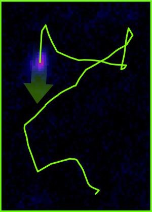
Bacteria perform run-and-tumble motion in a liquid medium, as described in the seminal tracking experiments by Berg and Brown [7], Macnab and Koshland [22] (see also Berg’s book [6]). They alternate between so-called run phases of ballistic motion (say, with velocity ), and tumble phases of rotational diffusion (Figure 1). Fast reorientation of the cell occurs during tumble. After tumbling, bacteria make a new run with another velocity . For the sake of simplicity, we assume that tumbles are instantaneous reorientation events, where the cell changes velocity from to . On the other hand, duration of each run phase is a random time. It is assumed to follow an exponential distribution with heterogeneous rate . By modulating the time of runs, bacteria are able to distinguish between favourable and unfavourable directions. This strategy based on temporal-sensing chemotaxis allows them to navigate in heterogeneous environments.
The tumbling frequency distribution can be decomposed as
for some probability density function , satisfying . The kernel describes the distribution of post-tumbling velocities.
Following [27, 28], we make the hypothesis that runs are modulated by two chemoattractant signals. We denote by the concentration of some amino-acid released by the bacterial population (e.g. aspartate, serine). We denote by the concentration of some nutrient consumed by the bacterial population (e.g. oxygen, glucose).
We assume that both signals have an additive effect on temporal sensing. Furthermore, they proceed with the same signal integration function , with possibly different relative amplitudes . Accordingly, the tumbling frequency reads
| (1.2) |
where denotes the material derivative along the direction . Chemotaxis is positive when is globally decreasing (tumbling is more likely when the concentration of chemoattractant is decreasing).
Equation (1.1) is complemented with two reaction-diffusion equations for both chemical concentrations ,
| (1.3) |
where are positive constants, denoting respectively the diffusion coefficient of , the diffusion coefficient of , the rate of degradation of , the rate of production of by the bacteria, and the rate of consumption of the nutrient by the bacteria. In addition, denotes the spatial density of bacteria,
1.2. Chemotactic waves in micro-channels
Concentration waves of chemotactic bacteria E. coli were described in the seminal article by Adler [1]. They inspired the second article of Keller and Segel about mathematical modelling of chemotaxis [20]. We refer to [31] for a featured review on the mathematical modelling of these chemotactic waves. Mesoscopic models describing this remarkable propagation phenomenon were proposed independently in [34], and [27, 28]. Relevance of modelling at the mesoscopic scale relies on tracking experiments. They reveal the directional distribution of individuals, and in particular the spatially dependent biases in the trajectories.
Model (1.1)-(1.2)-(1.3) has been validated on some experimental data in [28], whereas its macroscopic diffusive limit has been validated in [27] on some other experimental set. It is worth noticing that the diffusive regime is valid when the chemotactic biases are small. This is not the case in the experiments presented in [28]. We believe that in the latter, the mesoscopic scale is more appropriate to describe the bacterial population dynamics.
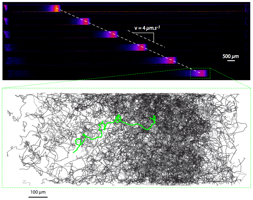
Experimental setting described in [27, 28] is as follows: cells (approx. bacteria E. coli) are initially located on the left side of a micro-channel after centrifugation. The width of the micro-channel is , the height is , and the total length is . The time span of experiments is about a few hours. After short time, a significant fraction of the population moves towards the right side of the channel, at constant speed, within a constant profile (see Figure 2).
The goal of the present work is to construct travelling waves for the run-and-tumble equation, coupled to a pair of reaction-diffusion equations (1.1)-(1.2)-(1.3). This is an original result, up to our knowledge. Note that equation (1.1) is conservative. Hence, such travelling waves are in some sense solitary waves. They are very different from reaction-diffusion travelling waves that occur in the Fisher-KPP equation, for instance (see e.g. [15, 21, 4]).
1.3. Simplifying modelling assumptions
The construction of travelling waves for the system (1.1)-(1.2)-(1.3) requires some modelling simplifications. One crucial assumption is about the signal integration function . In order to maintain the spatial cohesion of the band, it is important that the function has a sharp transition for small temporal variations. Accordingly, we make the following choice
This relies on some well documented amplification mechanism, see [6, Chapter 11. Gain Paradox]. This specific choice imposes conditions on the pre-factors , for the frequencies to be non-negative, namely .
We further ignore any delay effects during the signal integration process, as the tumbling rate is a function of the time derivative (1.2). This is to say that bacteria are supposed to react to instantaneous variations of signal. This assumption is very restrictive, as compared to experimental data [29, 6]. However, including any memory effect, as in [13, 34, 25] would make the analysis much more difficult. This is left for future perspective.
In addition, assume that the post-tumbling velocity is drawn uniformly at random,
| (1.4) |
Assumption (1.4) ignores angular persistence during tumbling, as opposed to experimental evidence [6].
Finally, we restrict to dimension , as we are looking for planar waves.
We discuss possible relaxations of these assumptions in Section 8.
1.4. The measure on the velocity set
We deal with two classes of probability measures separately, namely the case of a continuum of velocities, and the discrete case.
1.4.1. The continuous case
- (A1):
-
is absolutely continuous with respect to the Lebesgue measure. Moreover, the probability density function belongs to for some . Precisely, we have:
We do not include the case , for technical reasons that involve Hölder regularization by averaging lemma. On the other hand, the case is also excluded in the course of analysis, as it is borderline. However, it is included in the final result because any p.d.f. having a compact support belongs to all spaces.
Examples:
the projection of the uniform measure on the unit circle onto the interval under the hypothesis of axisymmetry writes . This imposes . The same procedure in case of the unit sphere yields the uniform measure .
During the course of analysis, the following assumption will be required in order to refine the asymptotic decay of solutions.
- (A1’):
-
In addition to (A1), the p.d.f. is bounded below by some on .
Example:
the projection of the uniform measure on the two-dimensional unit ball onto the unit interval under the hypothesis of axisymmetry writes . It belongs to , but it vanishes on . Similarly, the same procedure in case of the the three-dimensional unit ball yields .
1.4.2. The discrete case
- (A2):
-
is a finite sum of dirac masses,
The latter assumption is motivated by numerical analysis, where are quadrature weights. This case is not included in the main result. However, comprehensive numerical analysis performed in Section 7 enables to find counter-examples for the existence and uniqueness of travelling waves. This completes our main result, as it shows that additional conditions on the parameters are mandatory, on the contrary to the macroscopic model obtained in the diffusion limit (see Section 2.1).
A companion paper develops accurate well-balanced schemes for solving the Cauchy problem [9]. Consequences of the lack of existence and uniqueness are investigated in the long-time asymptotic of (1.1)-(1.2)-(1.3). We also refer to [26, 14, 35] for numerical analysis of variants of (1.1), based either on Monte Carlo simulations, or inverse Lax-Wendroff methods.
1.5. Notations and conventions
As the problem is linear with respect to the cell density , we can normalize the latter to have unit mass,
| (1.5) |
The space variable in the moving frame at speed is denoted by .
We denote by the maximal velocity.
We assume that the amplitude of the tumbling rate is without loss of generality.
We adopt the following convention: the superscripts + and - denote the position of the velocity with respect to the speed (resp. and ), whereas the subscripts + and - denote the relative position with respect to the origin (resp. and ). For instance, denotes the density of bacteria on the right side (), moving towards the origin (). Similarly, denotes the spatial density of the same group of bacteria.
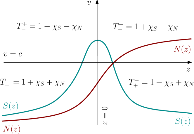
The tumbling rate can take only four values , depending on the sign of the gradients. Due to the particular ansatz that underlies the existence of travelling waves, is can only change value if crosses , or if crosses the origin. Accordingly, the four possible values are denoted by . We refer to (3.3), and Figure 4 for the rule of signs.
We also denote in short the effective chemotactic biases on each side of the origin.
We denote by the Hölder semi-norm.
1.6. Existence of travelling waves
We address the existence of travelling wave solutions for the coupled problem (1.1)-(1.2)-(1.3). The wave speed is denoted by , and the spatial coordinate in the moving frame is denoted by . We keep the notation for some particular solution of (1.1) of the form . Travelling waves are solutions of the following stationary problem in the moving frame,
| (1.6) |
where the tumbling rate is given by
| (1.7) |
Note that we have reduced to without loss of generality. Also, we restrict to the case in order to fix the global direction of the wave.
As the measure may vary during the analytical procedure, it is fruitful to write a weak formulation of the first equation in (1.6), so that the role of the measure clearly appears.
Definition 1.1 (Weak formulation).
A weak solution of the first equation in (1.6) is such that for all test function ,
| (1.8) |
We begin with the existence of stationary clusters, in the absence of nutrient.
Theorem 1.2 (Stationary cluster).
Assume , and . Under assumption (A1), there exist symmetric, positive functions solution of the stationary wave problem
Assume in addition that (A1’) is satisfied. Then, there exists an exponent , and a velocity profile such that (resp. ) converges exponentially fast to as (resp. to as ).
In order to establish our main result, existence of travelling waves driven by consumption of the nutrient, we need to impose some extra conditions on the parameters. As the conditions are not simple to state, we refer to the lines of the proof for the details.
The first two conditions are linked with the coupling with . The first condition (6.5) writes
| (1.9) |
where is defined implicitly such that
and is the smallest positive root of
The second condition (6.6) writes,
| (1.10) |
where is defined implicitly such that
and is the smallest positive root of
The third condition (6.7) is related to the coupling with . It reads
| (1.11) |
where and are the smallest positive roots of, respectively,
Remark 1.3.
Theorem 1.4 (Travelling wave).
Assume . Under assumption (A1), and conditions (1.9)-(1.10)-(1.11), there exist a non-negative , and positive functions solution of the travelling wave problem (1.6)-(1.7).
Assume in addition that (A1’) is satisfied. Then, there exist two exponents , and two velocity profiles such that (resp. ) converges exponentially fast to as (resp. to as ).
As mentioned above, the discrete case (A2) is not included in Theorem 1.4. Nonetheless, it will be discussed with lots of details in Section 7.
Counter-examples for both existence and uniqueness of the travelling waves have been found numerically, based on the analysis performed in Section 7.
1.7. Acknowledgements
The author is indebted to B. Perthame who introduced him to kinetic equations with applications in chemotaxis, and biology in general. This work originated from a fruitful collaboration with J. Saragosti, A. Buguin and P. Silberzan. The author is grateful to N. Bournaveas, C. Emako, and N. Vauchelet for preliminary discussions about this work. He has benefited from stimulating discussions with E. Bouin, N. Caillerie, F. Golse, G. Raoul, Ch. Schmeiser, M. Twarogowska, and J. Vovelle. The author is particularly grateful to L. Gosse for his enlightening explanation of the numerical analysis of (1.1).
This work was supported by the LABEX MILYON (ANR-10-LABX-0070) of Université de Lyon, within the program ”Investissements d’Avenir” (ANR-11-IDEX-0007) operated by the French National Research Agency (ANR). This project has received funding from the European Research Council (ERC) under the European Union’s Horizon 2020 research and innovation programme (grant agreement No 639638).
2. Sketch of proof
As the complete proof of Theorem 1.4 is quite technical, the strategy of proof is sketched below. We begin with the corresponding macroscopic problem, obtained in the diffusion limit. The latter is by far easier to handle with. This will drive the analysis at the mesoscopic scale. Then, we draw two main obstacles arising at the mesoscopic scale. Section 2.2.2 contains the main argument to overcome the first obstacle in full generality. The second obstacle yields restriction on the parameters, as conditions (1.9)-(1.10)-(1.11).
2.1. Construction of travelling waves at the macroscopic level
The formal diffusion limit of (1.1), derived when the biases are small, is given by the following drift-diffusion/reaction-diffusion coupled system [27],
| (2.1) |
Let recall the existence and uniqueness of one-dimensional solitary waves.
Theorem 2.1 ([27]).
There exist a speed , and two positive values , such that the system (2.1) admits travelling wave solutions with the following boundary conditions:
Assume in addition that changes sign only once, and that is positive everywhere. Then, the speed is uniquely determined by the following implicit relation,
| (2.2) |
Remark 2.2.
We believe that there cannot exist travelling waves for which (or ) changes sign several times. Alternatively speaking, we conjecture that uniqueness holds true in Theorem 2.1 without extra conditions, up to standard transformations (multiplication by a constant factor, translation, symmetry).
It is instructive to recall the proof of Theorem 2.1, as it will guide the proof of Theorem 1.4. The former is based on explicit computations. However, this will no longer be the case at the mesoscopic level.
Proof.
Firstly, system (2.1) is written in the moving frame . We keep the notations for the unknown functions.
| (2.3) |
The starting point consists in assuming that the communication signal reaches a unique maximum, say at , and that the nutrient is increasing. The validation of this ansatz a posteriori, will set the equation for (2.2).
This ansatz determines the sign of the chemical gradients. It enables to decouple the drift-diffusion equation from the reaction-diffusion system in (2.3). Accordingly, the cell density is solution of the following equation,
The density profile is explicitly given as a combination of two exponential distributions,
| (2.4) |
We denote , and the exponents on both sides. We impose positivity of both exponents, .
In a second step, the concentration is computed through the elliptic equation,
| (2.5) |
The solution is given by , where is the Green function associated with the elliptic operator . We have
The exact value of the normalization factor does not matter here. We introduce , and the exponents on both sides.
On the other hand, according to the general result stated in Proposition 5.1 below, the monotonicity of is basic, i.e. first increasing, then decreasing, just because is so. However, the change of monotonicity is not necessarily located at , as in the initial ansatz.
The quantity enables to locate the maximum of . If , then reaches its maximum for , whereas if , then reaches its maximum for . According to the previous ansatz, the maximum of must be located at .
Consequently, we need to compute the value of , denoted by , in order to validate the initial ansatz. We have,
It is immediate to see that the function is decreasing with respect to , as the ratio is decreasing ( is decreasing, whereas is increasing), and the ratio is increasing ( is increasing, whereas is decreasing). Analysis of the extremal behaviours reveal that there is indeed a unique root of . Moreover, it belongs to the interval . Indeed, we have , but . Therefore, . On the other hand, we have , since , whereas .
2.2. Main obstacles at the mesoscopic level.
When trying to mimic the previous proof at the mesoscopic level, several difficulties arise. Some are technical, and dedicated tools from kinetic theory can overcome them (e.g. averaging lemma). However, at least two main obstacles require much more work. We describe them below. The first obstacle can be resolved in full generality. However, the second obstacle requires additional conditions on the parameter. This is the main reason why Theorem 1.4 is more restrictive than its macroscopic version Theorem 2.1.
2.2.1. Non monotonicity of the mesoscopic density with respect to .
As emphasized in Section 2.1, the construction of travelling waves for the macroscopic problem relies on the fact that changes sign exactly once. To summarize, it is consistent to assume that changes sign exactly once, say at w.l.o.g. Then, explicit computations prove that reaches its maximum value at the same location. It is an immediate consequence that , being solution of the elliptic problem (2.5) with as a source term, has a unique critical value, corresponding to a maximum for . However, this might not coincide with . In fact, there is a unique such that the maximum of is located at .
We follow the same approach at the mesoscopic level. We freeze and , simply assuming the same monotonicity conditions as above. Then, we solve in the first line of system (1.6), and we deduce the spatial density . At this stage, however, it is not immediately clear that , being solution of the same elliptic problem (2.5) with as a source term, has a unique critical value. This would hold true provided has basic monotonicity (increasing, then decreasing), as in the macroscopic case. In fact, such monotonicity would be an equivalent requirement, without any extra condition on and , since the Green function converges to a Dirac mass for and .
The first major problem can be rephrased as follows:
Let be the density obtained from the first equation in system (1.6) under the hypotheses that changes sign at only, and is positive. Prove that is increasing for , and decreasing for .
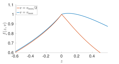
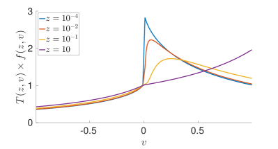
Obviously, the monotonicity of , say for all , would follow from the monotonicity of , if we were able to show that for all , and all . However, the latter is not expected to hold true in full generality, as can be seen on numerical simulations for large, , and accordingly (see Figure 3). Therefore, the monotonicity of for can only result from compensations when integrating with respect to velocity.
Our problem can be recast as follows,
Let be the density obtained from the first equation in system (1.6) under the hypotheses that changes sign at only, and is positive. Describe the velocity profiles in order to show that compensations yield the appropriate monotonicity for when integrating with respect to velocity.
It turns out that such compensations always occur, with no additional condition on the parameters. We are able to prove that inappropriate monotonicity of may arise for large positive velocities (for ). However, it is compensated by small positive velocities. Moreover, negative velocities contribute with the appropriate sign. We shall decipher velocity profiles in order to capture these compensations.
2.2.2. Non monotonicity of the location of the maximal value of with respect to .
The conclusion of the proof of Theorem 2.1 is facilitated both by the monotonicity of , and by the unambiguous extremal behaviours (, ).
It turns out that, none of these two facts is generally true at the mesoscopic level. The corresponding function may vary in a non monotonic way, so that it crosses several times. This clearly prevents uniqueness of the speed .
On the other hand, there exists a range of parameters for which , and , where is the maximal admissible value for . Furthermore, for all admissible values of . This prevents existence of travelling waves in our framework.
2.3. Strategy of proof
Here, we sketch briefly the argument for resolving the first issue raised in Section 2.2.1.
We use a kind of homotopy argument, by deforming the measure . If is a symmetric combination of two Dirac masses, this is the two velocity case, which is very similar to the macroscopic problem, for which monotonicity is straightforward, see (2.4). When the support of is concentrated around two symmetric velocities, it is not difficult to prove that monotonicity still holds true.
As changes continuously, we establish that cannot change monotonicity. There is some subtlety here because does not appear in the kinetic equation in (1.6). The natural macroscopic quantity to look at is indeed the density of tumbling events per unit time, namely
| (2.6) |
so that the first line in (1.6) can be rewritten as
| (2.7) |
The function can be reconstructed entirely from by the Duhamel formulation along characteristics lines, for :
| (2.8) |
and similarly for .
The integral quantity (2.6) is a combination of the integral over , and the integral over , with different weights (, see Figure 4). Accordingly, we focus on the quantities
because they are common to both and , according to the following rules
The key point is to establish the following enhancement of monotonicity:
Assume that both and satisfy
Then inequalities in the large are in fact strict inequalities. Therefore, and necessarily keep the same monotonicity as the measure varies continuously.
As mentioned in Section 2.2.1, it is mandatory to understand compensations through the refined description of velocity profiles. The argument goes as follows, say for . Assume that both and are non-increasing functions. We deduce from the Duhamel formula (2.8) that for . Therefore,
On the other hand, we have
| (2.9) |
The quantity has no sign in general, but we are able to prove that, whenever it has the inappropriate sign (here, positive), this can happen for large velocities only. Due to the decreasing weight in the integral formula (2.9), the following deduction holds true,
On the other hand, we deduce from the very definition of (2.6) that
The latter quantity is negative because for . QED
Of course, there is some additional work to ensure that monotonicity is indeed the appropriate one for large , in order to get enough compactness in the argument. Also, regularity of the macroscopic quantities is required in order to justify the use of differential calculus.
3. Preliminary results
In this section, we make the following a priori hypotheses which enable to decouple system (1.6):
| (3.1) |
Accordingly, we are reduced to examine the following linear equation,
| (3.2) |
where , with the sign convention as follows (see also Figure 4),
| (3.3) |
3.1. Solution of the uncoupled problem
Throughout this section, we assume that is satisfied. We shall make clear why we need uniform boundedness from below on the support of . Assumption (A1’) will be removed later on by some approximation procedure, at the expense of missing the refined asymptotic description of the solution as .
We proceed as in [10], where the existence of a stationary density solution to (3.2) is established in the case , and accordingly . Here, this result is extended to the asymmetric case , and . We also refer to a more recent work [23] that extends this confinement result to the higher dimensional case.
Theorem 3.1 (Exponential confinement by biased velocity-jump processes).
Let . Assume . Assume that is satisfied. There exists a density solution of (3.2). Moreover, there exist two exponents , and two velocity profiles such that (resp. ) converges exponentially fast to as (resp. to as ).
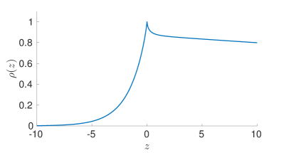
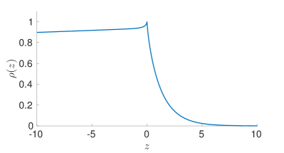
The extremal values and are defined precisely during the course of the proof (3.8)-(3.12). The condition guarantees that . On the other hand, if, and only if, . For values of outside , the solution does not decay exponentially, either on the left, or on the right side (see Figure 5).
Proof.
As stated in the Theorem, we restrict here to the continuous setting, under Assumptions . The case of discrete velocities (A2) can be solved directly by a finite dimensional approach based on Case’s normal modes, see Section 7.1.
Step #1. Identification of the asymptotic profiles. We make the following ansatz for large (positive) ,
where
| (3.4) |
and is characterized by the following relation,
| (3.5) |
The latter relation determines a unique positive , under the restriction that on the support of , provided that the mean algebraic run length is negative in the moving frame, i.e.
| (3.6) |
Indeed, the function
is continuous, and increasing. Moreover, as is bounded below on , it diverges to when attains the maximal possible value ensuring , i.e. (recall that is the maximal velocity). Moreover, the value at coincides with the mean algebraic run length (3.6).
Remark 3.2 (About the additional condition (A1’) on ).
If vanishes on the boundary of , say at , then it may happen that converges to a finite negative value, as converges to . Then, the formal ansatz for the velocity profile (3.4) must be corrected with a Dirac mass, as follows,
| (3.7) |
where is defined so as to compensate the negativeness of the integral, namely (3.5) rewrites as,
We refer to [8], where a similar issue was identified and resolved, in the large deviations asymptotic of a basic kinetic model, namely the BGK equation.
Noticeably, the asymptotic profile proposed in the formal ansatz (3.7) is not a bounded function. This is clearly an obstacle in using the approach developed below, which requires uniform boundedness of . To overcome this issue, we shall derive uniform estimates for at further stage, independently of any bound on from above, see Section 3.2.
On the other hand, condition (3.6) determines a minimal admissible value for . More precisely, is defined as the critical speed such that the mean algebraic run length vanishes,
| (3.8) |
To see this, let introduce the function , defined as follows,
| (3.9) |
It is continuous and decreasing with respect to . Indeed, in the case (A1), the derivative writes
The last contribution is written formally. However, it can be shown that it vanishes by approximation of the Dirac mass via mollifiers, provided that for (111Take an approximation of the Dirac mass, then ).
By examining the limiting cases, we deduce that there is a unique such that . Notice that the sign of is the same as the sign of , which is the same as the sign of by symmetry of :
| (3.10) |
We make a similar ansatz for large (negative) ,
where
The rate of exponential decay is uniquely determined by the following relation,
provided that the mean algebraic run length is positive in the moving frame, i.e.
| (3.11) |
Again, this determines a maximal admissible value , because the mean algebraic run length is positive for , and the dependency with respect to is Lipschitz continuous and decreasing. More precisely, it is defined as
| (3.12) |
Notice that both depend on . For the sake of clarity, we may omit this dependency in the notation. From now on, we assume that the speed belongs to the interval , and we keep in mind the extremal behaviours,
Alternatively speaking, the spatial density becomes flat on the far right side as the speed decreases to , whereas it becomes spatially flat on the far left side as it increases to (see Figure 5). This property will play a crucial role in the last step of the proof, when determining the speed for the coupled problem.
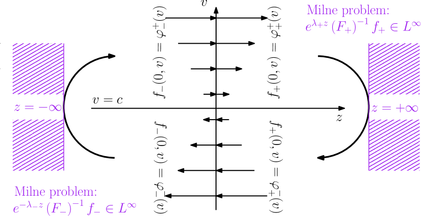
Step #2. Connection with the Milne problem. One key observation is that the function verifies a kinetic equation on the half space , which satisfies the maximum principle,
| (3.13) |
However, we have no idea yet about the incoming data, i.e. the inward velocity profile at : . For the ”boundary value” at , we only impose boundedness of . This prescribes uniquely as a solution of the so-called Milne problem in radiative transfer theory [5]: being given the inward velocity profile for , there exists a unique , such that
Moreover, we deduce the following bound from the maximum principle (see [10] for details),
We apply the same construction for negative . We define accordingly , which solves a similar problem,
together with the matching inward velocity profile, i.e.
We refer to Figure 6 for a sketch of the construction of both and starting at with boundedness reflection at on both sides.
Step #3. A fixed point argument. We define the linear map as follows,
so as being a fixed point is equivalent to closing the loop , see Figure 6.
Compactness is required in order to apply the Krein-Rutman theorem. It can be deduced from classical averaging lemma, since the outward velocity profile is given by
| (3.14) |
where the macroscopic quantity is defined as,
One-dimensional averaging lemma [5] guarantees that has Hölder regularity (see also the proof of Proposition 3.3#2).
As a consequence, has Hölder regularity too. Alternatively speaking, negative velocities at necessarily emerge after some tumbling event, for which regularization occurs via velocity averaging. Similarly, has Hölder regularity on . Hence is a compact map. On the other hand, positivity is an immediate consequence of the Duhamel formula (3.14).
Applying the Krein-Rutman theorem, there exists a velocity profile , associated with a dominant eigenvalue such that . We deduce that from the conservation laws
| (3.15) |
Indeed, we have
Step #4. Refined asymptotic behaviour as . The zero rate of decay is a trivial solution of the l.h.s. of (3.5). It corresponds to a flat mode which is excluded to ensure integrability of . It comes with the conservation of flux (3.15). Besides, the non trivial, positive root comes with another conservation law. By multiplying (3.13) against , we obtain
since , and . We define accordingly such that
| (3.16) |
Then, it is possible to prove exponential decay towards the asymptotic profile as using second order entropy method with respect to the space variable. In fact, the two auxiliary quantities
and
satisfy the following system of (in)equalities,
| (3.17) |
where
We refer to [10] for further details. The system (3.17) can be turned into the following second-order damped differential inequality,
Using the ”boundary condition” , we deduce that there exists a constant depending on , and , such that,
As a conclusion, we have obtained the following weighted estimate,
| (3.18) |
Intuitively, is an estimate of the spectral gap in the spatial decay. Loosely speaking, we have,
A similar estimate holds true for . ∎
3.2. Regularity (uniform with respect to )
We investigate the regularity of the macroscopic quantity
from which the solution can be reconstructed entirely by the Duhamel formulation along characteristics lines (2.8).
In brief, we obtain that all quantities are smooth expect possibly at , and at . More precisely, assuming that , the following properties hold true:
-
•
is continuous with respect to , for all ,
- •
-
•
the spatial density is smooth on both sides of the origin. Noticeably, may have a logarithmic singularity at the origin. This singularity plays some important role in the analysis.
Proposition 3.3.
Assume that is normalized to have unit mass (1.5). Then is uniformly bounded, and exponentially decreasing as . Moreover, these two estimates are uniform with respect to , the lower bound on .
Proof.
We develop a bootstrap argument, focusing on the regularity of . The first immediate observation is that , more precisely .
Step #1. is uniformly bounded. We start from the self-convolution structure of . Indeed, we deduce from (2.8) that we have for ,
| (3.19) |
On the other hand, we have
| (3.20) |
We define accordingly the two auxiliary functions
Lemma 3.4.
Let such that (A1). Then there exist positive constants and such that
Remark 3.5.
In the case , the first item should be replaced with a logarithmic growth, i.e. .
Proof.
We deduce from the Hölder inequality that,
In the case , i.e. , we clearly have everywhere since the first integral is convergent as . We get immediately exponential decay for some absolute for large , say . In the case , then the integral is not convergent as , but is equivalent to for some constant .
Similar estimates hold true for . ∎
Lemma 3.4 is useful because it enables to reformulate (3.19)–(3.20) as follows
with for . Similarly, we have
Fix to be chosen later. The first iteration of the bootstrap argument yields
and also
where we have simply used in the first contribution.
Similar estimates hold true on the negative side, for . Thus, we can prove that belongs to .
Then, we proceed recursively, in order to gain integrability in a finite number of iterations. We get immediately the following recurrence formula,
| (3.21) |
The analogous one for requires one more argument because the transfer term from negative to positive side is not of convolution type. Indeed, we have
Now, back to the proof of Lemma 3.4, we realize that
| (3.22) |
where we impose the constraint , to ensure . We deduce,
| (3.23) | ||||
provided that the following condition is fulfilled,
to get integrability of the first contribution in the r.h.s. of (3.23). This last inequality holds true when satisfies the recurrence relation (3.21), because .
Now, choose such that is the smallest integer larger than . Then the recurrence relation on (3.21), with the initial condition , guarantees that , i.e. . In fact, the last step of the iteration should be done with caution. At the step, we have obtained . Young’s inequality still holds, namely (it is simply Hölder’s inequality here). However, the estimate (3.22) becomes
The last contribution is bounded since . This procedure enables to bootstrap from to in a finite number of iterations, provided .
As a corollary, we get that is uniformly bounded too. This is a direct consequence of the Duhamel formulation (2.8),
Step #2. is Hölder continuous. We apply one-dimensional averaging lemma [17]. For , we have
By choosing , we obtain
| (3.24) |
Note that in the case (), we cannot get any Lipschitz estimate, but there is a logarithmic correction. However, this is not important for the remaining of this work.
Step #3. is exponentially decaying. Recall that the maximum principle for the normalized solution yields the following estimate,
| (3.25) |
The key point is that, although may not be uniformly bounded with respect to (see Remark 3.2), it happens surely for . Therefore, is uniformly bounded. Of course, this does not control all velocities uniformly with respect to , but this is yet an important information.
Next, we use the additional conservation law (3.16). It reads
| (3.26) | ||||
The last quantity is uniformly bounded, because is defined such as (3.5). In order to control the exponential decay of from (3.26), it remains to control small relative velocities, i.e. . But this is guaranteed by the pointwise estimate (3.25) which reads as follows,
| (3.27) |
The function possibly diverges only at in the limit , see (3.7). On the other hand, the obvious estimate ensures that there exists such that is uniformly bounded on .
3.3. Further regularity
We can obtain better regularity for (resp. ) by bootstrap. This will be needed in Section 4, as we shall compute derivatives of with respect to .
First, we establish that is Hölder continuous with respect to both . We use the formulation of along characteristic lines (2.8). Let . We have successively
and
The Hölder regularity of the exponential function with respect to is evaluated as follows,
We deduce the following Hölder regularity for ,
We notice that regularity of degenerates as . We will see a more quantitative feature of this degeneracy in Lemma 4.8 below. Now, we are in position to improve slightly the regularity of , locally uniformly for . We perform the same computation as (3.24):
| (3.28) | ||||
Therefore, we have gained regularity, since . However, this is clearly not uniform up to due to the pre-factor.
It is possible to iterate the whole argument, in order to prove that belongs to the family of Hölder spaces , with , for all . Indeed, at the next step, the same lines of calculation yields
and
| (3.29) |
The last integral contribution can be evaluated as follows,
| (3.30) |
Combining (3.29) and (3.30), we deduce
The last inequality is a consequence of . Then, we update the Hölder estimate (3.28) to
Iteratively, for all , we obtain the existence of such that
| (3.31) |
A similar result holds true on the negative side, i.e. for .
We can establish the following result as a by-product of this recursive Hölder regularity.
Proposition 3.6.
The macroscopic quantities (resp. ) are Lipschitz continuous, locally uniformly on (resp. on ).
Proof.
Firstly, we transfer the macroscopic Hölder regularity (3.31) to partial Hölder regularity with respect to velocity. We have successively, for ,
| (3.32) |
and for ,
Let be the exponent such that , and to be chosen below. The Hölder regularity of the exponential function with respect to is evaluated as follows,
Consequently, we deduce:
| (3.33) |
Combining (3.32) and (3.33), we obtain eventually,
| (3.34) |
Secondly, we compute directly the derivatives of and , based on (2.7):
We observe that for , , as can be seen directly on (2.8). We have as well. In the latter case, the condition is crucial. Consequently, we can use the Hölder regularity of , with respect to velocity (3.34), so as to get
Therefore, it is sufficient to choose large enough such that , in order to ensure integrability in the r.h.s., and thus boundedness of the derivative of . The same estimate holds true for , and also on the negative side .
Note that can be chosen almost arbitrarily at this stage. The next result will impose some condition on it. ∎
Remark 3.7.
There is some subtlety in the last argument, as it may not be legitimate to take the limit if . To circumvent this small issue, it is possible to extend the formula along characteristic lines (2.8) for all . This leads to a non optimal result, as the density is certainly smooth if is outside .
The next corollary is the last step of our bootstrap argument. Such regularity will be required in the proof of Lemma 4.11.
Corollary 3.8.
The derivative of the macroscopic quantity (resp. ) is Hölder continuous, locally uniformly on (resp. on ).
Proof.
Recall that has been chosen such that . Let belong to . By differentiating (2.8) with respect to , we obtain successively
and
Note that the condition is compulsory for the integrability of at . All in all, we get eventually,
| (3.35) |
3.4. Regularity within exponential tails
We derive regularity estimates for the normalized density , defined as follows,
| (3.37) |
For the sake of simplicity, we assume in this section that the p.d.f. is bounded below and above: there exists such that
| (3.38) |
In fact, the results derived afterwards will be used under this restrictive condition (Lemma 4.6). The key observation is that satisfies the following equation for ,
| (3.39) |
and similarly for . We deduce from (3.25)-(3.27) that is uniformly bounded (recall that is bounded under the condition (3.38)). Hence, the r.h.s. of (3.39) is uniformly bounded. We deduce from the one-dimensional averaging lemma that is almost Lipschitz continuous, namely,
| (3.40) |
With this estimate at hand, it is possible to reproduce the estimates of Section 3.3, with the tumbling rate , which is bounded below and above. Notice that it is not even necessary to iterate the argument in order to obtain Lipschitz regularity as in Proposition 3.6. Indeed, we have obviously , since we assume . We cannot readily choose in the estimates because of the logarithmic correction in (3.40), but taking any is sufficient for our purpose. Note also that the calculation leading to Hölder regularity with respect to velocity, as in (3.34), requires some adaptation because the new tumbling rate has a linear dependency with respect to . But this additional contribution is partially Lipschitz continuous, so that it does not affect the conclusion.
Corollary 3.9.
Under the additional condition (3.38), the macroscopic quantities are Lipschitz continuous, locally uniformly on , and the normalized densities are Hölder continuous with respect to velocity locally uniformly on . More precisely, for all , and , there exists a constant such that for all ,
and similarly for .
4. Monotonicity of the macroscopic quantities ,
4.1. Monotonicity of .
Let , and define as in Theorem 3.1. The aim of this section is to establish monotonicity of some macroscopic quantities, despite the lack of monotonicity of with respect to space variable (see Figure 3).
We recall the notation , resp. . Accordingly, we have
| (4.1) |
The following theorem is the cornerstone of the present study.
Theorem 4.1.
Under the assumptions of Theorem 3.1, both and are decreasing for . Reversely, and are increasing for .
We split the proof into several steps. We begin with an easy case, when is close to the symmetric combination of two Dirac masses. Then, we deform continuously the measure , and check carefully that none of the macroscopic quantities can change monotonicity. This requires many technical estimates in order to control the continuous deformation of .
Step #1. Initialization (the easy case). We first state a proposition establishing monotonicity under the very restrictive condition that the measure is concentrated around two symmetric velocities . In the extreme case where
| (4.2) |
the conditions (3.6) and (3.11) which are required for exponential decay on both sides, read as follows,
| (4.3) |
They are equivalent to the following conditions, provided that ,
Hence, it is required that belongs to the interval . Note that the latter is not empty since .
Proposition 4.2 (The approximate two velocity case).
Let be such that both conditions in (4.3) are satisfied. Assume that the support of is contained in , where , for small enough. Then is decreasing for (resp. increasing for ).
Proof.
The key observation is that the equilibrium of the model with only two velocities (4.2) can be computed explicitly. In this case, has the expected monotonicity. The computations are facilitated by the fact that , since the flux (3.15) vanish at equilibrium.
If is not too far from , then the same result should hold, using again the fact that the flux is identically zero at equilibrium. This is indeed the case,
| (4.4) |
where is arbitrary, and denote the average with respect to measure . On the support of , we find as ,
| (4.5) |
where the sign is determined by the sign of . We seek a condition on such that the r.h.s. of (4.5) is always negative. The following two inequalities should hold, corresponding to the two possible choices of sign,
| (4.6) |
Clearly, such a real number exists if, and only if,
We find that this is equivalent to the first condition in (4.3). Within this choice of , we deduce easily from (4.4)-(4.5) that is decreasing, provided that is small enough.
The same holds true for , with possibly another choice of constant . ∎
Step #2. Enhancement of monotonicity. The next proposition is the crucial step in the proof. It includes the cancellation property that accounts for the compensations in the velocity profile.
Proposition 4.3 (Enhancement of monotonicity).
Assume that is non-increasing (resp. is non-decreasing). Then monotonicity turns out to be strict. Moreover we have the following stronger set of inequalities,
Proof.
We prove this statement by deciphering the shape of the velocity profile .
We consider first . The easiest part of the statement concerns negative relative velocities, : by integration along the characteristics (2.8), we obtain
| (4.7) |
This quantity is clearly increasing with respect to , provided that is non-increasing, and non constant on for all . This is indeed the case by assumption.
Similarly, is decreasing with respect to , for , and .
Let introduce the notation . Interestingly, the stationary equation (2.7) is rewritten as
| (4.8) |
From (4.7) we also get the following inequality:
| (4.9) |
We deduce immediately that the density is decreasing, since the combination of (4.8) and (4.9) implies that
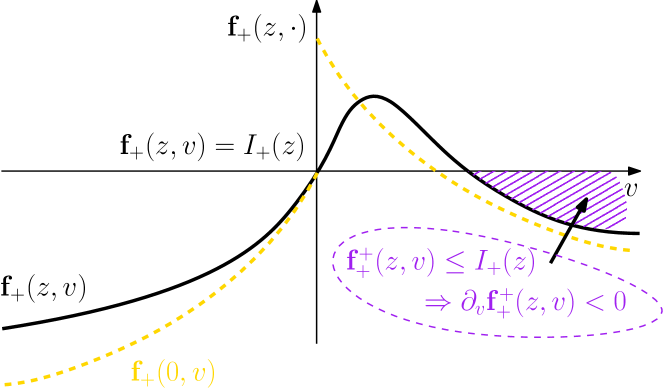
The case of positive relative velocities requires more work. Indeed, the velocity profile is not necessarily monotonic for , on the contrary to (see Figures 3 and 7). However, we are able to establish the following properties, which are sufficient for our purpose.
Lemma 4.4.
The function is decreasing with respect to on the set . As a consequence, for all there exists such that for , and for .
Note that we allow for . In the latter case, for all .
Proof.
The function satisfies the following damped transport equation with a non-negative source term,
By solving this transport equation along characteristics lines, it is immediate to establish that, if , then for all . On the contrary, if , then for all .
Take . We have
Introduce . It satisfies the following damped transport equation with source term,
| (4.10) |
If is such that , then for all . On the other hand, we clearly have since
| (4.11) |
(recall that is decreasing with respect to , for , and ).
We deduce from (4.10) and (4.11) that for all as soon as . Therefore, for all , . As a consequence, the function is decreasing with respect to on .
The velocity threshold is constructed by choosing the smallest velocity such that . ∎
To conclude the proof of Proposition 4.3, we establish that is decreasing as well, using compensations between lower and higher velocities. The derivative writes
| (4.12) |
The key observation is that, were we ignoring the factor inside the integral, the r.h.s. in (4.12) would be
| (4.13) |
by the very definition of . Indeed, it is negative since for all (4.9).
It is sufficient to show that the r.h.s. of (4.12) can be handled in the same way, because lower velocities contribute more to the integral, and because the inappropriate sign is contributed by higher velocities according to Lemma 4.4. After integration by parts, we obtain
| (4.14) | ||||
| (4.15) |
Notice that integration by parts makes sense here since the possibly singular term at in (4.14) vanishes because pointwise for . Hence,
As in the proof of Proposition 3.6, we find that taking large enough, the latter contribution converges to 0 as .
We deduce from (4.13) that the first contribution in (4.15) is negative. On the other hand, the cumulative function
is everywhere negative. Indeed, according to Lemma 4.4, this cumulative function is decreasing, then increasing (and possibly only decreasing) on . Therefore, it reaches its maximum value at or at . Since it vanishes at and it is negative at (4.13), it is everywhere non positive.
As a conclusion, both contributions in (4.15) are negative, so is decreasing. ∎
Remark 4.5.
As can be observed on Figure 3, the threshold velocity is increasing with respect to . We present briefly a formal proof of this secondary statement. For the sake of simplicity, let assume that all quantities, including have regular variations with respect to . We differentiate the relation with respect to ,
However, by definition of , and equation (4.8). Therefore,
since is decreasing at .
This illustrates the fact that the monotonicity of is getting better and better as increases, since the zone with inappropriate monotonicity shrinks (and may eventually disappears as in Figure 3). Hence, the lack of monotonicity of is clearly a consequence of overshoot phenomena around the origin where all signs are changing in the tumbling rate .
Step #3. Propagation of monotonicity. In the last step, we propagate the monotonicity of along a continuous deformation of the measure . Let be a path of probability measures satisfying Assumption (A1), continuous for the strong topology of , and satisfying the following properties:
Here, is a non-increasing, continuous function such that , where is chosen according to Proposition 4.2. Note that by definition of . However, it may happen that crosses . At this point, the regularity of degenerates. We shall analyse carefully this point (see Lemma 4.8). Besides, this careful analysis brings some useful quantitative information.
We shall prove that for all , is decreasing on , and increasing on . First, we can deduce from the refined asymptotic of obtained in Theorem 3.1 that this is true for large , with some quantitative estimates which are locally uniform with respect to .
Lemma 4.6 (Asymptotic monotonicity).
Let . There exists , such that
where .
Proof.
We restrict to . The procedure for is the same. We omit the dependency upon in the notation for the sake of clarity.
We control explicitly the behaviour of as (3.18). Recall the definitions of (3.16),
| (4.16) |
Let introduce the corrector such that
| (4.17) |
The latter bound requires some improvement, as it controls the norm of with a weight, whereas some unweighted bound would be more appropriate for our purpose. This is done as follows (recall the pointwise decay bound (3.27)),
| (4.18) |
where .
Recall the calculation of the derivative of ,
| (4.19) |
Integrating (4.17) against with respect to velocity, we obtain
(recall that by definition). On the other hand, we have the pointwise identity,
By construction, we have
The latter has the sign of . Thus, we would be in position to conclude from (4.19), if we could abusively neglect the corrector terms, as follows,
However, the pre-factor in (4.19) makes the estimate involving the corrector more difficult to handle with.
We proceed as follows to circumvent this issue. For , we have
The three contributions are estimated as follows. From Corollary 3.9, we deduce
On the other hand, we have
Finally, we deduce from the bound (4.18) that
Collecting , we get eventually an estimate of the form ,
| (4.20) |
It remains to bound uniformly from below in order to conclude. This is the purpose of the next auxiliary lemma.
Lemma 4.7.
Under the unit mass normalization (1.5), the positive numbers and are bounded below by some positive constant.
Proof.
We begin with the bound on , by using the conservation law (3.16),
Integrating this inequality with respect to , we obtain
| (4.21) |
where denotes the mass which is contained on the positive half space, namely
Note that in the last estimate, we have used the uniform exponential decay of (3.27). The same estimate holds true on the negative half space,
| (4.22) |
Combining (4.21) and (4.22), we obtain using the notation ,
| (4.23) |
Eventually, we get that is bounded from below under the normalization (1.5), and the conditions , .
The estimate on from below is obtained with the same lines of proof,
This concludes the proof of Lemma 4.7. ∎
Lemma 4.6 has a counterpart for small . Indeed, we expect from Section 3.3 that regularity of cannot be guaranteed up to (see Proposition 3.6). The case of small requires particular attention. In the next lemma, we investigate quantitatively the behaviour of macroscopic quantities for small . In fact, we prove that it may happen that the derivative of diverge as , but with the appropriate sign.
We face the following trivial alternative: either the derivative of diverges, or it has a finite value, and we can push regularity up to the origin. This depends whether (), or not. In order to make it quantitative, so as to manage the transition between the two alternatives, we distinguish between the three following cases:
-
(i)
, i.e. ,
-
(ii)
,
-
(iii)
None of (i)-(ii), i.e. .
Here, is a positive real number to be defined below.
Lemma 4.8.
Let . Assume (i) or (ii). There exist and such that
On the contrary, assume (iii). Then, (resp. ) is Lipschitz continuous on (resp. on ), with quantitative bounds depending on .
Proof.
The computation of the derivative of goes as follows,
We deduce from global Hölder regularity of both and that,
The constant that pops up in the leading order contribution has a sign. Interestingly, this sign is the signature of the confinement effect at the origin .
Lemma 4.9.
The quantity is bounded from below by a positive constant, uniformly for .
Proof.
First, we compute explicitly the value of this quantity, by means of . From (4.1) evaluated at , we deduce
| (4.24) |
Then, we seek some quantitative estimate of from below. Recall the Hölder regularity of . By definition, we have
Using the bound from below on obtained via other arguments (4.23), we deduce the statement of Lemma 4.9. ∎
We deduce that for small enough, we have
Assume condition (i) i.e. . Then, the last integral is equivalent to as . Therefore, there exists , and , such that for .
Assume condition (ii) i.e. . Then, for , we have
The latter inequality determines the choice of , so that the contribution on the r.h.s. is controlled by some negative constant .
Assume condition (iii). Then, the a priori control enables to revisit regularity of . Indeed, we get immediately from (2.7) that is Lipschitz continuous with respect to , uniformly with respect to . Differentiating with respect to , for only (since is discontinuous with respect to ), we deduce that is also Lipschitz continuous with respect to . So is .
This concludes the proof of Lemma 4.8. ∎
After the quantitative control of at both ends and , we can initiate the homotopy like argument. Let introduce the set
| (4.25) |
We shall prove that is both open and closed in . As it is non-empty by Proposition 4.2, it coincides with .
Lemma 4.10.
is closed in .
Proof.
The stationary distribution associated with the probability measure is unique in the space (up to a constant multiplicative factor), where the weight is defined by
This is a consequence of the linear and irreducible structure of the kinetic equation(222A much more refined analysis based on hypocoercive estimates after [11] is developed in [10] for the Cauchy problem, in the symmetric case and . There, the goal is to capture exponential relaxation in time towards the stationary state. Of course, this ensures uniqueness as a weak corollary.). Let be two stationary distributions belonging to , and denote . By integration of the difference equation against , we obtain successively,
Using equation (2.7) satisfied by the function , we find,
Hence, there exists a function of the variable only, say , such that . Plugging this identity into the stationary equation, we find . The unit mass normalization (1.5) enables to fix this multiplicative factor to 1.
Continuity of with respect to is a consequence of this uniqueness property. Let . The sequence is uniformly bounded, uniformly Hölder continuous with respect to , and Hölder continuous with respect to , locally uniformly with respect to . Moreover, it is uniformly exponentially small for large (see Proposition 3.3). By a diagonal extraction argument, there exists a subsequence that converges towards some function . Convergence is uniform on compact sets of .
On the other hand, in by the continuity assumption. Therefore, we can pass to the limit in the weak formulation (1.8)
We deduce from the uniqueness of the stationary distribution that .
To conclude, it is sufficient to notice that (resp. ) is a sequence of non-increasing functions (resp. non-decreasing functions) which converges pointwise towards (resp. ). Therefore, is non-decreasing (resp. is non-increasing). ∎
Lemma 4.11.
is open in .
Proof.
Some stability result in Lipschitz regularity is required to ensure that certainly remains uniformly negative, on compact sets of (recall that we control the asymptotic behaviour as ).
Let . Proposition 4.3 ensures that for all , and for all . Let large enough so that the quantities arising in Lemma 4.6 have the appropriate sign for close to and , i.e. both
Our claim is the following: there exists and a neighbourhood of such that
| (4.26) |
Otherwise, there would exist a sequence converging towards such that the maximum value of (resp. minimum value of ) converges to a non-negative value. We restrict to for the sake of clarity. Let be a maximum point.
To control the possible singularity at the origin, we distinguish between the two alternatives (i) or (ii), and (iii), as discussed in Lemma 4.8.
In cases (i) or (ii), we can separate from the origin, say , as the derivative is uniformly negative close to the origin. Note that the continuity of the support of is implicitly used in this argument.
On the other hand, we learn from Corollary 3.8 that is uniformly Lipschitz continuous on . By compactness of , and equi-continuity of , we can pass to the limit along some subsequence, so as to obtain
for some which is a limit point of . This is a contradiction. The same holds for .
In case (iii), regularity is fine up to , so we can apply the same argument with , including the origin.
Therefore, (4.26) holds true, and is open. ∎
We are in position to conclude the proof of Theorem 4.1. Indeed, for all , the macroscopic quantities and satisfy the appropriate monotonicity condition (4.25). This monotonicity condition remains true in the limit , as in the proof of Lemma 4.10. By approximation, it is true for all measure satisfying hypothesis (A1).
4.2. Improved monotonicity and quantitative regularity
Several corollaries can be deduced from the previous monotonicity analysis. A first result improves monotonicity properties of the macroscopic densities .
Corollary 4.12.
Let be the normalized density defined as in (3.37),
| (4.27) |
Let and . Then has the same monotonicity as :
Proof.
We introduce a pair of exponents , and . We shall prove that the monotonicity property holds true for all such pair By increasing up to we will obtain Corollary 4.12 as a limiting result.
With some abuse of notation, we still denote by the density normalized with exponents as in (4.27). It satisfies the following equation,
where satisfies the following identity,
There, we have used the zero-flux property of the stationary state (3.15). The same holds for , and . We introduce the new tumbling rates
We sketch briefly how to adapt the three steps in the proof of Theorem 4.1.
Step #1. Initialization (the easy case). Notice that . We repeat computation (4.4):
To conclude as in Section 4.1, we seek satisfying the following pair of conditions, instead of (4.6):
Existence of is equivalent to the following inequality,
| (4.28) |
Recall the equation for the right side exponent (3.5), when the measure is a symmetric combination of two Dirac masses (4.2):
We deduce that
Plugging this identity into (4.28), we obtain the equivalent formulation,
The last condition clearly holds true, as by definition.
Step #2. Enhancement of monotonicity. Now, assume a priori that is non-increasing, and that is non-decreasing.
The shapes of the velocity profiles of are the same as for .
-
(i)
For and , is non-decreasing with respect to . Moreover, we have . Indeed, we have
(4.29) Thus, is decreasing. A similar statement holds true for (), and .
-
(ii)
For and , is decreasing with respect to on the set . Indeed we adapt the two ingredients of the proof of Lemma 4.4. Firstly, satisfies a damped transport equation with a non-negative source term,
Secondly, introduce the auxiliary function . It satisfies the following damped transport equation with source term,
The same conclusion as in Lemma 4.4 holds true. Therefore, the same compensations as in the proof of Proposition 4.3 are working to make decreasing too.
Step #3. Propagation of monotonicity. In order to conclude, it is sufficient to check that is uniformly decreasing as for large , as in Lemma 4.6. Again, the asymptotic behaviour of is involved. Roughly speaking, we have for ,
So, is decreasing with respect to for large , provided . This asymptotic result can be made quantitative and rigorous, as in Lemma 4.6.
On the other hand, the possible singular behaviour close to the origin, as in Lemma 4.8, is unaffected by the exponential normalization.
The following statement is an immediate consequence of Corollary 4.12.
Corollary 4.13.
For , we have
A similar statement holds true for .
Corollary 4.12 also enables to derive quantitative regularity estimates on macroscopic quantities.
Corollary 4.14.
The averaged quantity is Hölder continuous with some explicit constant which is linear with respect to (see (4.31) below).
Proof.
We restrict to the case . We argue as in the proof of Proposition 3.3 (3.24). Let . We have
We deduce from the Duhamel representation formula (4.29) that
On the other hand, for , we have
We deduce:
where the constant is defined as . Finally, we use the trivial relations and , in order to obtain the following estimate which is linear with respect to ,
By optimizing with respect to , we obtain the following quantitative Hölder estimate,
| (4.30) |
where
| (4.31) |
Note that the pre-factor is increasing, and satisfies for large . This rules out the Lipschitz case (), as expected from [17]. ∎
5. The case without nutrient (stationary cluster)
The existence of a stationary state is an immediate consequence of the monotonicity of established in Section 4, and the following general statement about solutions of the elliptic problem on . The purpose of this section is to deal with only. However, we formulate our statement for any to anticipate the coupling with the nutrient in the forthcoming section.
Here, we set , without loss of generality.
Proposition 5.1.
Assume that the function is locally Lipschitz continuous on , and that it is increasing for , and decreasing for . Let be the unique solution of the following elliptic problem
Then vanishes once, and only once.
Proof.
Let denote by the derivative of : . It belongs to , locally uniformly on . It satisfies the following equation,
together with the following asymptotic limits,
| (5.1) |
where the notation means that we approach from above, and means that we approach from below.
Assume by contradiction that vanishes at least twice. Then, we deduce from (5.1) that it must vanish at least three times, including a possible double root, where vanishes also. Two vanishing points are necessarily on the same side, say for . Accordingly, there must exist a locally minimal point with non positive value, , , and . If , or , we have
This is a contradiction. If , and then is necessary a double root. We can repeat the same reasoning on the right side: there must exist such that , , and . At this point, we have
Again, this is a contradiction. We argue similarly when we are to choose initially on the right side. ∎
6. Coupling with chemical concentrations (travelling wave)
6.1. Matching the condition on
As in the case without nutrient, we deduce from Proposition 5.1 that changes sign only once. However it might not happen at , as required in (3.1).
The objective of this section consists in varying such as to satisfy (similarly as in the proof of Theorem 2.1 in the macroscopic case).
This requires two intermediate results: continuity of as a function of , and analysis of the extremal behaviours as , resp. as .
We introduce the following notation for , as a function of parameter ,
Recall that is given by the following integral representation formula,
| (6.1) |
where the reaction-diffusion exponents are defined as
| (6.2) |
Proposition 6.1.
Under assumption (A1), the function is continuous on .
Proof.
Let . As in the proof of Lemma 4.10, we can extract a subsequence converging towards uniformly on compact sets of . First, we pass to the limit in the weak formulation
| (6.3) |
The l.h.s. can be handled easily as it can be written
The last contribution is bounded by . The r.h.s. in (6.3) must be treated with caution because is not continuous with respect to . However, we can split the integral into , and . The former is controlled by , the bound of , and the bound of . We can pass to the limit in the latter since provided .
By uniqueness of the limit problem, we have , where is the density profile associated with .
Finally, we can pass to the weak limit in the integral formula for (6.1). ∎
Proposition 6.2.
Under assumption (A1), there are explicit conditions on the reaction diffusion parameters such that the following extremal behaviours hold true,
The idea is quite simple: as , the macroscopic profile becomes flat on the right side (see Figure 5). As a result, we expect that the maximum of is pushed to the right of the origin, i.e. . Similar behaviour can be expected as , but on the right side. This is made as quantitative as possible in the following proof.
Proof.
We will use crucially the improved monotonicity obtained in Section 4.2, and particularly Corollary 4.13.
Firstly, we consider the case . We have
| (6.4) |
where is defined as in (4.16). In order to estimate from below, we use the improved regularity obtained in Corollary 4.14 (4.30). For all , we have
where the stopping time is given by
Similarly, for we find
where the stopping time is given by
Combining these two estimates, we get the following bound from below,
Plugging this estimate into (6.4), we deduce that there is an explicit constant such that
As , we have , and , therefore, the condition is a consequence of the following condition:
| (6.5) |
As the r.h.s. does not depend on the reaction-diffusion parameters , whereas the l.h.s. vanishes as , condition (6.5) is clearly not empty.
Secondly, we consider the case . There, we perform similar estimates, but the other way around,
where is defined as in (4.16). As previously, the ratio can be estimated from below by using the regularity of with respect to velocity, through the regularity of with respect to space. As a consequence, we get for ,
The latter is negative under some condition which reads,
| (6.6) |
We notice that the l.h.s. vanishes when , or (independently). This guarantees that the condition is not empty as well. ∎
6.2. Matching the condition on
The monotonicity condition on to be satisfied (3.1) is not very restrictive. It only requires as established in Proposition 6.3 below. This is automatically satisfied when , which is equivalent to (3.10), conditioned on (6.5)-(6.6).
On the contrary, if , then we should impose that in order to guarantee the existence of such that , conditioned on (6.6). Arguing as previously, a sufficient condition writes
which is equivalent to
| (6.7) |
To see that this condition is not empty, it is enough to consider that as . In a second step, the limit enables to realize the condition. However, this is not entirely satisfactory, as it imposes some strong condition on the parameters of the run-and-tumble process, .
We conclude this section by checking that, indeed, if , then is increasing.
Proposition 6.3.
Assume that , and that is exponentially bounded on both sides, namely
Then, there exist two constants , and a solution of the elliptic problem in (1.6), such that
Moreover, we have .
Proof.
We introduce . Elliptic equation for is equivalent to the following first order equation for ,
This rewrites as a non autonomous, non linear ODE in the variable,
| (6.8) |
together with the boundary conditions . This means that is the unique homoclinic orbit that leaves the origin as , and gets back to the origin as . A way to construct this solution is to consider the family of Cauchy problems on ,
| (6.9) |
and to take the limit as . Indeed, we deduce immediately from the structure of (6.9) that . In addition, we deduce from the Gronwall lemma that
As a consequence, for we deduce from Corollary 4.13 that
On the other hand, for , we deduce similarly that
In any case, we can extract a subsequence such that converges uniformly towards solution of (6.8) with the boundary conditions .
Previous estimates guarantee that is integrable on both sides, so it enables to define properly as in Proposition 6.3. ∎
This concludes the proof of Theorem 1.4.
7. Focus on the discrete velocity case
We revisit the travelling wave problem (1.6) in the discrete velocity case, under Assumption (A2). In this case, the auxiliary function is not continuous with respect to , but it has jumps each time crosses some discrete velocity . By analysing carefully the sign of the jumps, we are able to exhibit some set of parameters for which there is no uniqueness of the travelling wave. Interestingly, we can also find some set of parameters for which there is no travelling wave satisfying the natural ansatz (3.1).
The careful analysis of the discrete velocity case is based on the spectral decomposition of kinetic operators in Case’s elementary modes (see [19, 18] and references therein).
The extremal speeds are defined as in Section 3.1, see (3.8)-(3.12). There, the boundedness of the velocity measure is used. However, the auxiliary function is still decreasing, and Lipschitz continuous in the discrete velocity case (A2). The following computation resolves the case when crosses one of the discrete velocities . There, we have for sufficiently small,
Notice that the second contribution does not vanish here, on the contrary to the continuous velocity case (A1)(3.9), but it has the good sign to come up with the same conclusion since .
From now on, we suppose that , and that .
7.1. Spectral decomposition of kinetic transport operators
We develop in this section quantitative spectral analysis of the discrete velocity case (A2). Recall that we are seeking solutions of the linear equation
| (7.1) |
We decompose the solution on each side (resp. and ) along special Case’s solutions, which have the form
The total number of modes is . They are distributed on each side according to the position of relatively to the discrete velocities .
Definition 7.1.
Assume that is such that
| (7.2) |
-
(i)
There are negative modes defined for , , where , and are given by the following expressions,
Each exponent is a root of the following dispersion relation,
(7.3) -
(ii)
Similarly, there are negative modes defined for , , where , and are given by the following expressions,
Each exponent is a root of the following dispersion relation,
(7.4)
The following couple of propositions investigates the relation between the number of roots of the dispersion relations (7.3)-(7.4), and the degrees of freedom on the kinetic transport problems to be solved on each side. This discussion justifies a posteriori notations in the previous definition.
Proposition 7.2.
- (i)
- (ii)
Proof.
Let be defined as in (7.3) for ,
It is decreasing with respect to on each interval of definition. Moreover, we have since and as . We argue analogously for , by introducing as follows
Proposition 7.3.
-
(i)
Bounded solutions of the kinetic stationary problem (7.1) restricted to have exactly degrees of freedom. Any such solution can be decomposed uniquely as
(7.8) -
(ii)
Bounded solutions of the kinetic stationary problem (7.1) restricted to have exactly degrees of freedom. Any such solution can be decomposed uniquely as
(7.9)
Proof.
The number of degrees of freedom on is determined by the number of negative velocities (relatively to ), here . Indeed, analysis in Section 3.1 reveals that bounded solutions are entirely determined by the incoming velocity profile, corresponding to . A similar argument holds true for . ∎
In order to reconstruct an entire solution on , we shall solve a transfer eigenvalue problem. The continuity of at , , writes equivalently as follows,
| (7.10) |
This writes in matrix block form as follows
We realize immediately that a non-trivial solution exists, since the square matrix has a left eigenvector associated with eigenvalue zero:
where we have used both dispersion relations (7.3)-(7.4). We can characterize in a unique way, by prescribing a unit total mass (1.5),
Monotonicity of both and can be deduced from the results obtained in the continuous velocity case (A1), by approximation of the discrete measure by a sequence of absolutely continuous measures. Indeed, under the crucial assumption , regularity of the approximating sequence is guaranteed, provided it is chosen so as to avoid in its support. We are not aware of any direct argument based on the decomposition in Case’s modes (7.8)-(7.9).
7.2. Exchange of modes as crosses some discrete velocity
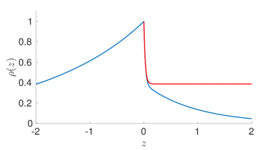
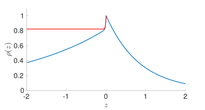
We investigate carefully the case where crosses one of the velocities , say , with increasing values. According to Section 7.1, there is a swap: one mode will disappear on the right side , this is mode , and one mode will appear on the left side, the new mode . The other modes will be essentially unchanged. During the swap, we expect a singular transition around the origin, as the largest exponents become arbitrarily large on both sides.
Proposition 7.4.
Assume crosses with increasing values. Then, for , we have
On the other hand, for , we have
The other roots have finite limits, denoted by (), which are roots of the function , obtained from by removing the term from the summation, and evaluating at .
Proof.
Limits exist by monotonicity of . For any , the limit is clearly finite by (7.5)-(7.6). Assume for instance that has finite limit as . Then, it should satisfy the relation
| (7.11) |
and so should the limits for . However, we deduce from Proposition 7.2 that relation (7.11) has only roots. Moreover, it cannot have a root larger than . This is a contradiction. We argue similarly for . ∎
The next result concerns the limit of the weights as . More precisely, we aim at describing the higher order contribution in the following decomposition of the spatial density in exponential modes (given here for ),
| (7.12) |
where we have opted for the notation . Interestingly, the contribution of the higher mode, here mode , has a non trivial contribution as . The same behaviour happens as . This emphasizes the dramatic discontinuity in the shape of the spatial profile as crosses the discrete velocity , as illustrated in Figure 8.
Proposition 7.5.
The weights have finite limits as , resp. as . The limits coincide up to a constant factor. In addition, has a finite limit which satisfies,
| (7.13) |
Similarly, has a finite limit which satisfies,
Proof.
Step #1. Firstly, we prove the existence of limits. For that purpose, we pass to the limit in the transfer matrix . We have
therefore,
| (7.14) |
where the question mark accounts for some undetermined limit. The left eigenvector associated with eigenvalue zero becomes
We deduce that the matrix obtained from (7.14) by eliminating row and column also possesses an eigenvector . Finally, the missing term can be recovered using the identity (7.10) for . In the limit , it becomes
We argue in a similar way in the case . Interestingly, the matrix is the same as when taking the limit from below . Therefore, the weights coincide up to a constant factor.
Step #2. Secondly, we prove that the limit (7.13) is positive. We consider the case where . We argue by computing the derivative of at in two different manners. Differentiating (7.12) with respect to , we obtain,
| (7.15) |
On the one hand, we notice that as . Indeed, we have
As a consequence, has a finite limit too. On the other hand, we learn from Section 4 that is decreasing. Dividing (7.15) by , then taking limit as , we get immediately
Furthermore, we can separate the respective contributions of positive relative velocities, and negative relative velocities, , as in the proof of Lemma 4.8. In particular, we have:
Recall the following identity from the proof of Lemma 4.9 (4.24),
We get eventually,
To conclude, recall from (7.6) that . This yields the following bound from below,
∎
7.3. Positive jumps in the function and consequences
In this section, we examine the matching condition on , namely
Our main objective is to investigate existence, and possible uniqueness of . As a matter of fact, we shall answer negatively to these questions, because the situation is by far more complicated than in the macroscopic diffusive limit discussed in Section 2.1.
In the following proposition, we establish that variations of can be deduced from some monotonicity of the macroscopic profile , with respect to . We include the dependency with respect to in the notations to resolve any possible ambiguity.
Proposition 7.6.
Suppose the profile has the following monotonicity,
| (7.16) |
then the function is decreasing.
Proof.
Recall that is given by the following integral representation formula,
| (7.17) |
where the reaction-diffusion exponents are defined as in (6.2). For our purpose, we compute
We integrate by parts the first contribution in each line of the r.h.s., in order to get the following expression,
| (7.18) |
To conclude it is sufficient to notice that
Therefore, all signs in (7.18) coincide to give
∎
Remark 7.7.
There is some ambiguity when we study the variation with respect to . Indeed, the profile is defined up to a constant factor. To resolve this ambiguity, notice that any smooth normalization of the type , , can be handled in the following way,
In particular, we see that when vanishes, so zeros of and do coincide.
Note that monotonicity condition (7.16) is exactly what is expected in the case of two velocities only . There, the spatial density is given by
where the exponents have the appropriate monotonicity with respect to (7.16), as in (7.7).
However, the situation is more tricky for a larger number of velocities, due to the superposition of modes, and in particular the breaking of monotonicity during exchange of modes, as in Figure 8. It can be seen in the latter that has exactly the reverse monotonicity with respect to , close to the origin (compare (7.16) and Figure 8). Of course, monotonicity (7.16) is recovered far from the origin, as the shape of is dominated by the lower mode.
The objective of the following calculation is to estimate the variations of as crosses some discrete velocity, following Section 7.2.
Firstly, we suppose that . We opt for the alternative formulation of after integration by parts in (7.17), and using the continuity of at ,
Taking the limit , we obtain
Similarly, we obtain after taking the limit ,
By taking the difference, we should pay attention to the fact that the averages and do not coincide, because there is one term changing in the sum, due to the discontinuity of . More precisely, we have
As a conclusion, we can decompose the jump in at into three different contributions,
Interestingly, the last line does not depend on the reaction-diffusion coefficients . On the other hand, the remainder is arbitrarily small as , for instance as , all other parameters being unchanged. In the latter case, the jump is positive as a consequence of Proposition 7.5 (see Figure 9).
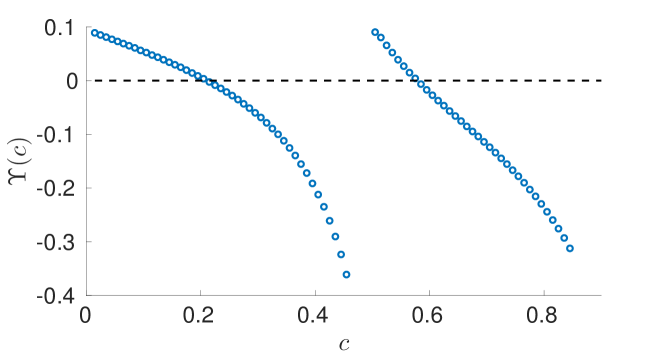
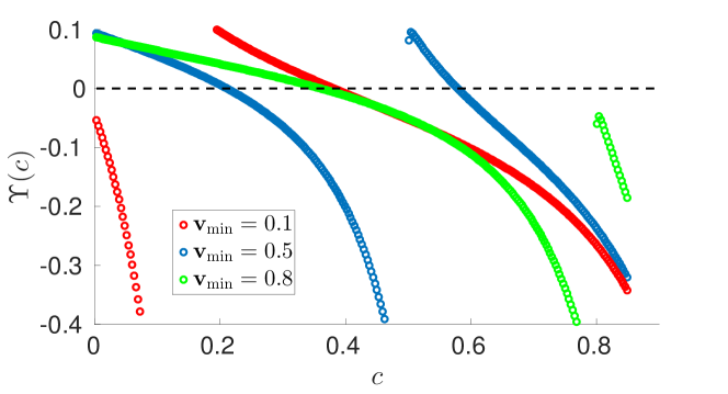
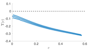
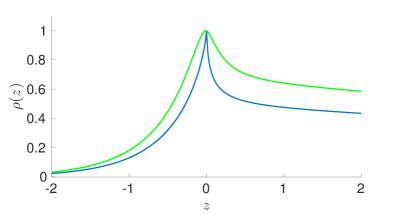
7.4. Numerical investigation
We conclude this section by some numerical illustrations.
Firstly, we investigate the case of four velocities, say . Figure 9 exhibits one particular case for which there is seemingly two roots of the matching equation . This is the exact counter-part of the exchange of modes happening when crosses the discrete velocity . There is a positive jump discontinuity in as . This corresponds precisely to the non-zero amplitude which is transferred instantaneously from the left to the right side of the origin as crosses . We believe that both travelling waves are stable (see [9] for more thorough discussion based on numerical experiments). This yields some interesting paradox (see Figure 10).
Secondly, we exhibit another intriguing case, with a larger number of velocities (an idealization of the continuous case) for which there is seemingly no solution to the matching equation (Figure 11). The long time behaviour of the Cauchy problem is very difficult to conceive in the mind.
8. Perspectives
8.1. Moderate signal integration
It would be interesting to include more functions than the sign function in (1.2) during the course of analysis. Indeed, a more appropriate choice would be a decreasing sigmoidal function with a stiffness parameter that is a typical time-scale [28],
Time can be related to the adaptation time-scale of individual cells [25].
There are two important differences with the analysis performed here: first, the tumbling rate cannot be reduced to an elementary rule of signs. Also, the confinement effect is more involved, as the rate of confinement strongly depends on the asymptotic decay of chemical concentrations.
8.2. Delay effects during signal processing
Clearly, the assumption of instantaneous signal integration is very reductive. A way to relax this strong assumption consists in including more variables in the kinetic model, accounting for signal processing at the level of individual cells [13, 34, 16, 33, 25]. However, this makes the analysis much more complicated. Reduced model different from (1.1) could be investigated first.
8.3. Angular persistence
By relaxing the specific choice (1.4), angular persistence during tumbling can be taken into account. In fact pre- and post-tumbling velocities are correlated. The mean value of the directional change is approx. [6, 28]. This can be encoded in the model using a Gaussian p.d.f. to distribute the post-tumbling velocity, namely
In [28], it has been further evidenced that the standard deviation itself is modulated by the chemical gradients, as predicted in [32]. This can be put into the model via the dependency , where is an increasing function of the tumbling rate : more likely is the tumble, larger the deviation between and is expected.
8.4. Two-species concentration waves
In [2, 12], the authors investigate a two-species model for the interaction of two populations of bacteria with different intrinsic wave speeds. The analogue of the diffusive limit system (2.1) is analysed by seeking travelling wave solutions. As far as we know, the corresponding kinetic system has not been studied yet.
References
- [1] J. Adler. Chemotaxis in Bacteria. Science, 153(3737):708–716, Aug. 1966.
- [2] L. Almeida, C. Emako, and N. Vauchelet. Existence and diffusive limit of a two-species kinetic model of chemotaxis. arXiv:1404.4769 [math], Apr. 2014.
- [3] W. Alt. Biased random walk models for chemotaxis and related diffusion approximations. J. Math. Biol., 9(2):147–177, Apr. 1980.
- [4] D. G. Aronson and H. F. Weinberger. Multidimensional nonlinear diffusion arising in population genetics. Adv. Math., 30(1):33–76, Oct. 1978.
- [5] C. Bardos, R. Santos, and R. Sentis. Diffusion approximation and computation of the critical size. Trans. AMS, 284(2):617–649, 1984.
- [6] H. C. Berg. E. coli in motion. Springer, 2004.
- [7] H. C. Berg and D. A. Brown. Chemotaxis in Escherichia coli analysed by three-dimensional tracking. Nature, 239(5374):500–504, Oct. 1972.
- [8] N. Caillerie. Large deviations of a velocity jump process with a Hamilton-Jacobi approach. arXiv:1602.07216 [math], Feb. 2016. arXiv: 1602.07216.
- [9] V. Calvez, L. Gosse, and M. Twarogowska. Bi-stability of chemotactic bacterial waves: a numerical analysis. in preparation.
- [10] V. Calvez, G. Raoul, and C. Schmeiser. Confinement by biased velocity jumps: Aggregation of Escherichia coli. Kinetic and Related Models, 8(4):651–666, July 2015.
- [11] J. Dolbeault, C. Mouhot, and C. Schmeiser. Hypocoercivity for linear kinetic equations conserving mass. Transactions of the American Mathematical Society, 367(6):3807–3828, Feb. 2015.
- [12] C. Emako, C. Gayrard, A. Buguin, L. N. d. Almeida, and N. Vauchelet. Traveling Pulses for a Two-Species Chemotaxis Model. PLOS Comput Biol, 12(4):e1004843, Apr. 2016.
- [13] R. Erban and H. G. Othmer. From Signal Transduction to Spatial Pattern Formation in E. coli : A Paradigm for Multiscale Modeling in Biology. Multiscale Modeling & Simulation, 3(2):362–394, Jan. 2005.
- [14] F. Filbet and C. Yang. An inverse Lax–Wendroff method for boundary conditions applied to Boltzmann type models. J. Comput. Phys., 245:43–61, 2013.
- [15] R. A. Fisher. The Wave of Advance of Advantageous Genes. Annals of Eugenics, 7(4):355–369, 1937.
- [16] B. Franz, C. Xue, K. J. Painter, and R. Erban. Travelling Waves in Hybrid Chemotaxis Models. Bull Math Biol, 76(2):377–400, Dec. 2013.
- [17] F. Golse, P.-L. Lions, B. Perthame, and R. Sentis. Regularity of the moments of the solution of a Transport Equation. Journal of Functional Analysis, 76(1):110–125, Jan. 1988.
- [18] L. Gosse. Computing Qualitatively Correct Approximations of Balance Laws, volume 2 of SIMAI Springer Series. Springer Milan, Milano, 2013.
- [19] H. G. Kaper, C. G. Lekkerkerker, and J. Hejtmanek. Spectral methods in linear transport theory. Number v. 5 in Operator theory, advances and applications. Birkhäuser Verlag, Basel ; Boston, 1982.
- [20] E. F. Keller and L. A. Segel. Traveling bands of chemotactic bacteria: A theoretical analysis. J. Theor. Biol., 30(2):235–248, 1971.
- [21] A. Kolmogorov, I. Petrovsky, and N. Piskunov. Etude de l’équation de la diffusion avec croissance de la quantité de matière et son application à un problème biologique. Mosc. Univ. Bull. Math, 1:1–25, 1937.
- [22] R. M. Macnab and D. E. Koshland. The gradient-sensing mechanism in bacterial chemotaxis. Proceedings of the National Academy of Sciences, 69(9):2509–2512, 1972.
- [23] S. Mischler and Q. Weng. On a linear runs and tumbles equation. arXiv:1602.03474 [math], Feb. 2016. arXiv: 1602.03474.
- [24] H. G. Othmer, S. R. Dunbar, and W. Alt. Models of dispersal in biological systems. J. Math. Biol., 26(3):263–298, June 1988.
- [25] B. Perthame, M. Tang, and N. Vauchelet. Derivation of the bacterial run-and-tumble kinetic equation from a model with biochemical pathway. arXiv:1503.03979 [math], Mar. 2015.
- [26] M. Rousset and G. Samaey. Simulating individual-based models of bacterial chemotaxis with asymptotic variance reduction. Mathematical Models and Methods in Applied Sciences, 23(12):2155–2191, Nov. 2013.
- [27] J. Saragosti, V. Calvez, N. Bournaveas, A. Buguin, P. Silberzan, and B. Perthame. Mathematical Description of Bacterial Traveling Pulses. PLoS Comput. Biol., 6(8):e1000890, 2010.
- [28] J. Saragosti, V. Calvez, N. Bournaveas, B. Perthame, A. Buguin, and P. Silberzan. Directional persistence of chemotactic bacteria in a traveling concentration wave. PNAS, 108(39):16235–16240, Sept. 2011.
- [29] J. E. Segall, S. M. Block, and H. C. Berg. Temporal comparisons in bacterial chemotaxis. PNAS, 83(23):8987–8991, Dec. 1986.
- [30] D. W. Stroock. Some stochastic processes which arise from a model of the motion of a bacterium. Z. Wahrscheinlichkeitstheorie verw Gebiete, 28(4):305–315, Dec. 1974.
- [31] M. J. Tindall, P. K. Maini, S. L. Porter, and J. P. Armitage. Overview of Mathematical Approaches Used to Model Bacterial Chemotaxis II: Bacterial Populations. Bull. Math. Biol., 70(6):1570–1607, July 2008.
- [32] N. Vladimirov, D. Lebiedz, and V. Sourjik. Predicted Auxiliary Navigation Mechanism of Peritrichously Flagellated Chemotactic Bacteria. PLoS Comput Biol, 6(3):e1000717, Mar. 2010.
- [33] C. Xue. Macroscopic equations for bacterial chemotaxis: integration of detailed biochemistry of cell signaling. Journal of Mathematical Biology, Dec. 2013.
- [34] C. Xue, H. J. Hwang, K. J. Painter, and R. Erban. Travelling waves in hyperbolic chemotaxis equations. Bull. Math. Biol., 73(8):1695–1733, Oct. 2010.
- [35] S. Yasuda. A Monte Carlo simulation for kinetic chemotaxis models: an application to the traveling population wave. arXiv:1503.08099 [physics, q-bio], Mar. 2015. arXiv: 1503.08099.