Jeans Analysis for Dwarf Spheroidal Galaxies in Wave Dark Matter

Abstract

Although still under debate, observations generally suggest that dwarf spheroidal (dSph) galaxies exhibit large constant-density cores in the centers, which can hardly be explained by dissipationless cold dark matter simulations without baryonic feedback. Wave dark matter ($\psi{\rm DM}$), characterized by a single parameter, the dark matter particle mass $m_{\psi}$, predicts a central soliton core in every galaxy arising from quantum pressure against gravity. Here we apply Jeans analysis assuming a soliton core profile to the kinematic data of eight classical dSphs so as to constrain $m_{\psi}$, and obtain $m_{\psi}=1.18_{-0.24}^{+0.28}\times 10^{-22}\,\rm eV$ and $m_{\psi}=1.79_{-0.33}^{+0.35}\times 10^{-22}\,\rm eV~{}(2\sigma)$ using the observational data sets of Walker et al. (2007) and Walker et al. (2009b), respectively. We show that the estimate of $m_{\psi}$ is sensitive to the dSphs kinematic data sets and is robust to various models of stellar density profile. We also consider multiple stellar subpopulations in dSphs and find consistent results. This mass range of $m_{\psi}$ is in good agreement with other independent estimates, such as the high-redshift luminosity functions, the reionization history, and the Thomson optical depth to the cosmic microwave background.

1 Introduction

Dark matter, which constitutes $\sim 26\%$ of the total energy density (Planck Collaboration et al., 2015), plays an important role in the structure formation of the Universe. The conventional cold dark matter (CDM) model has been successful at explaining observations on large scales, such as cosmic microwave background (CMB) and large-scale galaxy structure resulting from primordial fluctuations (Tegmark et al., 2006; Cole et al., 2005; Frenk & White, 2012; Bennett et al., 2013). However, several discrepancies between observations and dissipationless CDM simulations on the galactic scale still persist. There are three major problems. (i) “missing satellite problem”: CDM simulations predict an order of magnitude more subhalos than observed satellite galaxies in the Milky Way (Klypin et al., 1999; Moore et al., 1999). (ii) “too-big-to-fail problem”: the average central density of the most massive CDM subhalos are significantly higher than that of the most luminous dwarf spheroidal (dSph) galaxies derived from their kinematic data (Boylan-Kolchin et al., 2012, 2011; Tollerud et al., 2012). (iii) “cusp-core problem”: CDM simulations predict a universal Navarro-Frenk-White (NFW) halo density profile (Navarro et al., 1997) with a cuspy central density, while observations of dSphs (Moore, 1994; Flores & Primack, 1994; Kleyna et al., 2002; Goerdt et al., 2006; Walker & Peñarrubia, 2011; Amorisco et al., 2013) and low surface brightness galaxies (de Blok et al., 2001; de Blok & Bosma, 2002; de Blok, 2005; Burkert, 1995; Borriello & Salucci, 2001; Oh et al., 2008) are, in general, better described by a cored density profile.

Generally speaking, there are two categories of solutions to these small-scale issues. The first class of approaches considers additional baryonic physics in CDM simulations, such as feedback from supernova explosions and stellar wind (Navarro et al., 1996; Read & Gilmore, 2005; Governato et al., 2010, 2012; Mashchenko et al., 2008; Pontzen & Governato, 2014), energy transfer from dynamical friction of compact baryonic objects (El-Zant et al., 2001), ram pressure stripping (Arraki et al., 2014), tidal stripping (Brooks et al., 2013), suppression of star formation rate by photoionization due to early reionization (Bullock et al., 2000; Benson et al., 2002; Somerville, 2002), blazer (Pfrommer et al., 2012), and cosmic-ray heating (Wadepuhl & Springel, 2011). See Weinberg et al. (2013) for a comprehensive review. The second class of approaches adopts alternative dark matter models, such as warm dark matter (Colín et al., 2000; Macciò et al., 2012; Lovell et al., 2012), self-interacting dark matter (Spergel & Steinhardt, 2000; Vogelsberger et al., 2012), and axion/scalar field dark matter (Turner, 1983; Khlopov et al., 1985; Sin, 1994; Guzmán & Matos, 2000; Peebles, 2000; Goodman, 2000; Hu et al., 2000; Matos et al., 2000; Sahni & Wang, 2000; Böhmer & Harko, 2007; Sikivie & Yang, 2009; Chavanis, 2011; Robles & Matos, 2013; Guth et al., 2015; Davidson, 2015), which naturally produce constant-density cores and a cut off in the matter power spectrum.

In this work, we focus on scalar field dark matter composed of extremely light bosons with negligible self-interaction, known as $\psi{\rm DM}$ (Schive et al., 2014a; Marsh & Silk, 2014) or fuzzy dark matter (Hu et al., 2000). In this scenario, dark matter consists of axion-like particles proposed by string theory (Arvanitaki et al., 2010; Svrcek & Witten, 2006) or non-QCD axions (Chiueh, 2014). By assuming a dark matter particle mass of $m_{\psi}\sim 10^{-22}\,\rm eV$, the de Broglie wave nature becomes manifest on astrophysical scale. Here uncertainty principle counters gravity below a Jeans scale, simultaneously leading to kpc-scale central density cores in dSph-sized subhalos and suppressing the abundance of subhalos with masses below $\sim 10^{10}\,M_{\sun}$ (Hu et al., 2000; Marsh & Ferreira, 2010; Schive et al., 2014a; Schive et al., 2014b). It thus provides a plausible solution to the small-scale issues in CDM. Moreover, on large scales $\psi{\rm DM}$ is statistically indistinguishable from CDM (Woo & Chiueh, 2009; Schive et al., 2014a; Marsh & Silk, 2014; Bozek et al., 2015; Widrow & Kaiser, 1993). For these reasons, $\psi{\rm DM}$ has become a viable candidate for dark matter.

One of the key features in $\psi{\rm DM}$ is that it has only one free parameter, $m_{\psi}$, the dark matter particle mass. It is thus crucial to validate whether the estimates of $m_{\psi}$ from various independent observational constraints are consistent with each other. Using CMB and galaxy clustering data, Hlozek et al. (2015) obtained $m_{\psi}>10^{-24}\,\rm eV$. Schive et al. (2016) used high-redshift galaxy luminosity function to derive $m_{\psi}>1.2\times 10^{-22}\,\rm eV$ (see also Bozek et al. (2015); Corasaniti et al. (2016)). Sarkar et al. (2016) used damped Lyman-$\alpha$ observations and found $m_{\psi}>10^{-23}\,\rm eV$. Marsh & Pop (2015) explored multiple stellar subpopulations in Fornax and Sculptor and estimated $m_{\psi}<1.1\times 10^{-22}\,\rm eV$. Lora et al. (2012); Lora & Magaña (2014) used the longevity of the cold clumps in Ursa Minor and Sextans and found $m_{\psi}\sim 0.3\--1\times 10^{-22}\,\rm eV$ and $m_{\psi}\sim 0.12\--8\times 10^{-22}\,\rm eV$, respectively. Using newly discovered ultra-faint dSphs, Calabrese & Spergel (2016) estimated $m_{\psi}\sim 3.7\--5.6\times 10^{-22}\,\rm eV$. According to these studies, which cover a variety of astrophysical probes, the viable $\psi{\rm DM}$ particle mass generally lies in the range $10^{-23}\--10^{-21}\,\rm eV$. See Marsh (2015) for a comprehensive review.

DSph galaxies are the most dark-matter-dominated systems with mass-to-light ratios exceeding $>100$ (Mateo, 1998; Kleyna et al., 2005) and with little gas and no recent star formation (Smecker-Hane et al., 1994; Tolstoy et al., 2003; Venn et al., 2004). Large spectroscopic surveys provide rich stellar kinematics and metallicity data of dSphs, allowing detailed studies on dark matter properties from dynamical modeling. We refer to Battaglia et al. (2013) for a comprehensive review on this subject. Several works suggest that the dark matter density profiles are cored rather than cuspy (Kleyna et al., 2003; Goerdt et al., 2006; Sánchez-Salcedo et al., 2006; Battaglia et al., 2008; Jardel & Gebhardt, 2012; Walker & Peñarrubia, 2011; Amorisco & Evans, 2012a), although debate still remains (Strigari et al., 2010, 2014; Jardel & Gebhardt, 2013). In this work, we apply Jeans analysis to the kinematic data of eight classical dSphs to determine $m_{\psi}$. Most importantly, we investigate (i) whether the estimates of $m_{\psi}$ from different dSphs are in good agreement with each other, and (ii) whether the combined constraint of $m_{\psi}$ from the eight classical dSphs is consistent with other independent observational constraints described previously.

The paper is structured as follows. We describe the procedure of our Jeans analysis in Section 2 and show results in Section 3. In Section 4, we address various uncertainties in the analysis and discuss some extended models. Finally, we summarize our findings in Section 5.

2 Jeans Analysis

In order to constrain the dark matter particle mass $m_{\psi}$ by the stellar kinematics of dSphs, we regard stars as tracers of the gravitational potential dominated by the dark matter and assume the tidal disturbance is negligible. Dynamical equilibrium of stars in dSphs is supported by velocity dispersion with negligible rotation (Mateo, 1998). Assuming spherical symmetry, the Jeans equation (Binney & Tremaine, 2008) relates the stellar phase-space distribution to the dark matter halo as

$$\frac{1}{\nu}\frac{d}{dr}(\nu\bar{v_{r}^{2}})+2\frac{\beta\bar{v_{r}^{2}}}{r}=-\frac{GM(r)}{r^{2}},$$ (1)

where $\nu(r)$, $\bar{v_{r}}(r)$, $\bar{v_{t}}(r)$, and $\beta(r)\equiv 1-\bar{v_{t}^{2}}/2\bar{v_{r}^{2}}$ are the stellar number density, radial velocity dispersion, tangential velocity dispersion, and orbital anisotropy, respectively. $M(r)$ is the enclosed mass of the dark matter. By assuming $\beta=\rm{constant}$, Equation (1) has the solution Łokas & Mamon (2003):

$$\nu\bar{v^{2}_{r}}=Gr^{-2\beta}\int_{r}^{\infty}s^{2\beta-2}\nu(s)M(s)ds.$$ (2)

By projecting Equation (2) along the line of sight, we get (Binney & Tremaine, 2008)

$$\sigma_{p}^{2}(R)=\frac{2}{\Sigma(R)}\int_{R}^{\infty}\biggl{(}1-\beta\frac{R^{2}}{r^{2}}\biggr{)}\ \frac{\nu\bar{v_{r}^{2}}r}{\sqrt{r^{2}-R^{2}}}dr,$$ (3)

where $R$, $\Sigma(R)$, and $\sigma_{p}(R)$ are the projected radius, stellar surface density, and line-of-sight velocity dispersion, respectively.

In the following, we address in detail (1) the dark matter mass profile in the $\psi{\rm DM}$ model, (2) the stellar density and velocity dispersion profiles in the Jeans analysis, and (3) the Markov chain Monte Carlo algorithm for constraining the posterior distribution of $m_{\psi}$.

2.1 Wave Dark Matter Halo

From numerical simulations, Schive et al. (2014a) found a gravitationally self-bound, constant-density core at the center of each $\psi{\rm DM}$ halo, which connects to an NFW profile at a larger radius. This cored profile satisfies a soliton solution and can be well fitted by (Schive et al., 2014a)

$$\rho_{\rm{soliton}}(r)=\frac{1.9~{}(m_{\psi}/10^{-23}\,\rm eV)^{-2}(r_{c}/\,\rm pc)^{-4}}{[1+9.1\times 10^{-2}(r/r_{c})^{2}]^{8}}~{}10^{12}\,M_{\sun}\,\rm pc^{-3},$$ (4)

which has two free parameters, $m_{\psi}$ and $r_{c}$, where $r_{c}$ is the core radius defined as the radius at which the density drops to one-half its peak value. The main goal of this work is thus to determine both $r_{c}$ and $m_{\psi}$ for each dSph. Note that the mass profile, $M(r)=4\pi\int_{0}^{r}s^{2}\rho(s)ds$, can be calculated analytically from Equation (4). See Appendix A for the explicit form.

Schive et al. (2014a) shows that, in general, the transition radius between the inner soliton and the outer NFW halo is greater that $3\,r_{c}$, which is a few times greater than the observed half-light radii of dSphs. It is therefore reasonable to assume that all stars reside within the central soliton and ignore the outer NFW halo in the first place when conducting the Jeans analysis. For dSphs with stars possibly extending beyond $3\,r_{c}$ (e.g., Fornax), we also extend the main analysis to include outer NFW halos (see Section 4.2).

2.2 Stellar Density and Velocity Dispersion

Stellar surface density of dSphs are commonly fitted by King, Sersic, or Plummer models (e.g., Irwin & Hatzidimitriou, 1995). Following Walker et al. (2009b), we first adopt a Plummer profile, $I(R)=L(\pi R_{h}^{2})^{-1}[1+R^{2}/R_{h}^{2}]^{-2}$, where $L$ is the total luminosity and $R_{h}$ is the radius enclosing $0.5\,L$. We use $R_{h}$ derived from Walker et al. (2009b). Further assuming a constant mass-to-light ratio, the three-dimensional density profile can be derived from the surface density profile by the Abel transform as $\nu(r)=3L(4\pi R_{h}^{3})^{-1}[1+r^{2}/R_{h}^{2}]^{-5/2}$. We also investigate other stellar density models in Section 4.1.2 so as to consolidate the results.

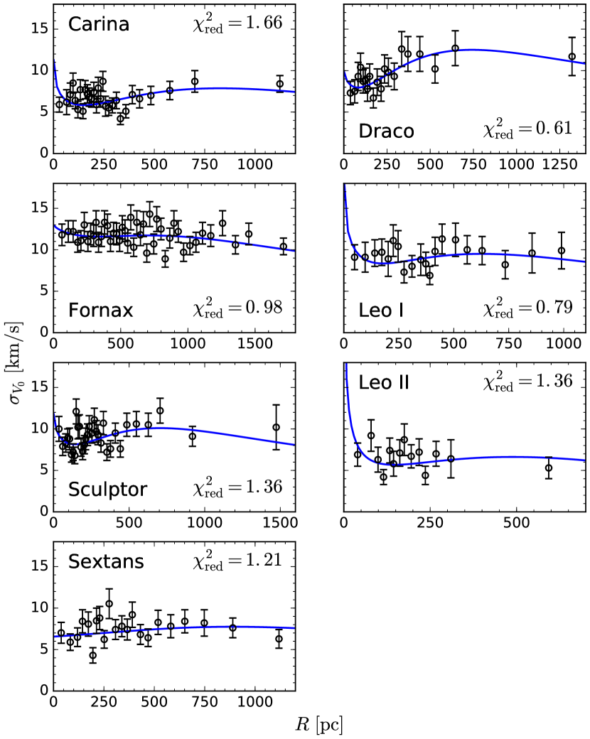
For the stellar velocity dispersion, we first adopt the data of eight classical dSphs in Walker et al. (2007) and Walker et al. (2009b); Walker (2013) (see Figs. 1 and 3), where the error bars indicate $1\sigma$ uncertainty. We shall also discuss the results using different observational data sets in Section 4.1.1.

2.3 Markov Chain Monte Carlo

To constrain the range of $m_{\psi}$, we follow Walker et al. (2009b); Salucci et al. (2012) and compare the empirical line-of-sight velocity dispersion, $\sigma_{V_{0}}(R_{i})$, with the projected velocity dispersion, $\sigma_{p}(R_{i})$, estimated from our Jeans analysis using Equation (3). We explore a three-dimensional parameter vector set $\vec{\theta}\equiv\left\{-\log_{10}(1-\beta),\,\log_{10}[r_{c}/\rm{pc}],\,\log_{10}[m_{\psi}/10^{-23}\rm{eV}]\right\}$ with uniform priors over the ranges $-1\leq-\log_{10}(1-\beta)\leq 1$, $1\leq\log_{10}[r_{c}/\rm{pc}]\leq 4$, and $0\leq\log_{10}[m_{\psi}/10^{-23}\rm{eV}]\leq 3$. We take the likelihood function

$$L(\vec{\theta})=\prod_{i=1}^{N}\frac{1}{\sqrt{2\pi\rm{Var}[\sigma_{V_{0}}(R_{i})]}}\exp\biggl{[}-\frac{1}{2}\frac{(\sigma_{V_{0}}(R_{i})-\sigma_{p}(R_{i}))^{2}}{\rm{Var}[\sigma_{V_{0}}(R_{i})]}\biggr{]},$$ (5)

where $\rm{Var}[\sigma_{V_{0}}(R_{i})]$ is the square of the observational uncertainty associated with $\sigma_{V_{0}}(R_{i})$ and $N$ is the number of bins in the velocity dispersion profile. We get a posterior probability distribution of each model parameter using a Markov chain Monte Carlo (MCMC) analysis with the Metropolis-Hastings algorithm (Metropolis et al., 1953; Hastings, 1970). We use the MCMC engine CosmoMC (Lewis & Bridle, 2002; Lewis et al., 2000) as a generic sampler and run four parallel chains. The code computes the R-statistic of Gelman and Rubin (An et al., 1998) as the convergence criterion and stops iterations when this value is less than 1.01 for each model parameter. The first $30\%$ accepted steps are discarded as burn-in.

To account for the observational uncertainty of $R_{h}$, we follow Salucci et al. (2012) and let $R_{h}$ sample randomly from a Gaussian distribution with mean and standard deviation equal to the observations (Irwin & Hatzidimitriou, 1995). We also investigate the case with a fixed $R_{h}$ in Section 4.1.2.

3 Results

We apply the Jeans analysis described above to the observational data of eight classical dSphs. Figure 1 shows the empirical velocity dispersions of Walker et al. (2009b, hereafter W09) and the estimated best-fit dispersions, which correspond to the maximum likelihood points in our MCMC chains with $m_{\psi}$ confined in the $2\sigma$ range of the combined constraint from eight dSphs. Clearly, the soliton core profile in the $\psi{\rm DM}$ model provides satisfactory fits to the observations. The reduced chi-square, $\chi_{\rm{red}}^{2}$, for each dSph assuming three free parameters lies in the range $0.26\--1.45$.

Figure 1: Projected velocity dispersion profiles for the eight classical dSphs in the observational data set of Walker et al. (2009b). Error bars show the empirical profiles with $1\sigma$ uncertainties. Solid lines show the best-fit profiles obtained in our Jeans analysis using the soliton density profile in $\psi{\rm DM}$ (Equation (4)), which provide satisfactory fits to the observations. The reduced chi-square, $\chi_{\rm{red}}^{2}$, of each dSph is also shown. The confidence intervals of the model parameters for each dSph are listed in Table 1.

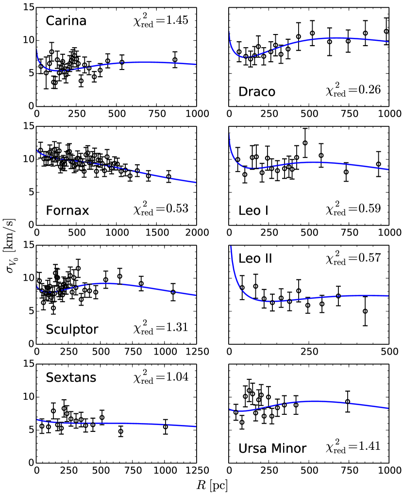
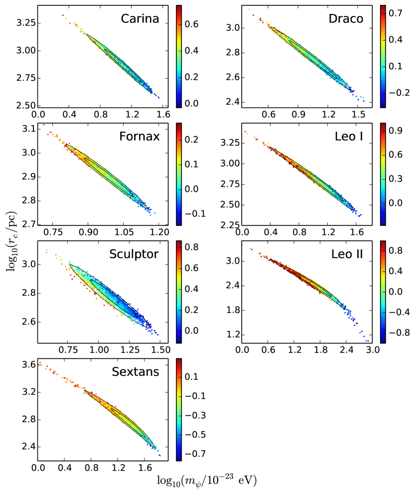
Figure 2 shows the $1\sigma\,(68\%)$ and $2\sigma\,(95\%)$ contours for the posterior distributions of $m_{\psi}$ and $r_{c}$. The corresponding values of $\beta$ are shown in the colored scatter plot. Notice that there is a clear correlation between $m_{\psi}$ and $r_{c}$. It results from the fact that a significant fraction of stars are located within the soliton core radius, where the dark matter density is roughly a constant and thus $m_{\psi}$ and $r_{c}$ become degenerate as $m_{\psi}\propto r_{c}^{-2}$ (see Equation (4)). It therefore relies on stars outside $r_{c}$ to break this degeneracy. The mean correlation is found to be $m_{\psi}\propto r_{c}^{-1.4}$, shallower than the fully degenerate case. It explains the tendency that the tangential anisotropy increases with decreasing $r_{c}$ and increasing $m_{\psi}$. By inserting $m_{\psi}\propto r_{c}^{-1.4}$ into Equation (4), we have $\rho_{\rm{soliton}}\propto r_{c}^{-1.2}$. Therefore, a smaller $r_{c}$ corresponds to a higher core density, which needs a larger amount of tangential anisotropy to counter gravity and match the observed velocity dispersion profile.

Figure 2: Posterior distributions of $m_{\psi}$ and $r_{c}$ colored by $\beta$ for each dSph in our MCMC analysis. Contours show the $1\sigma$ and $2\sigma$ confidence regions. The confidence intervals of the model parameters for each dSph are also listed in Table 1.

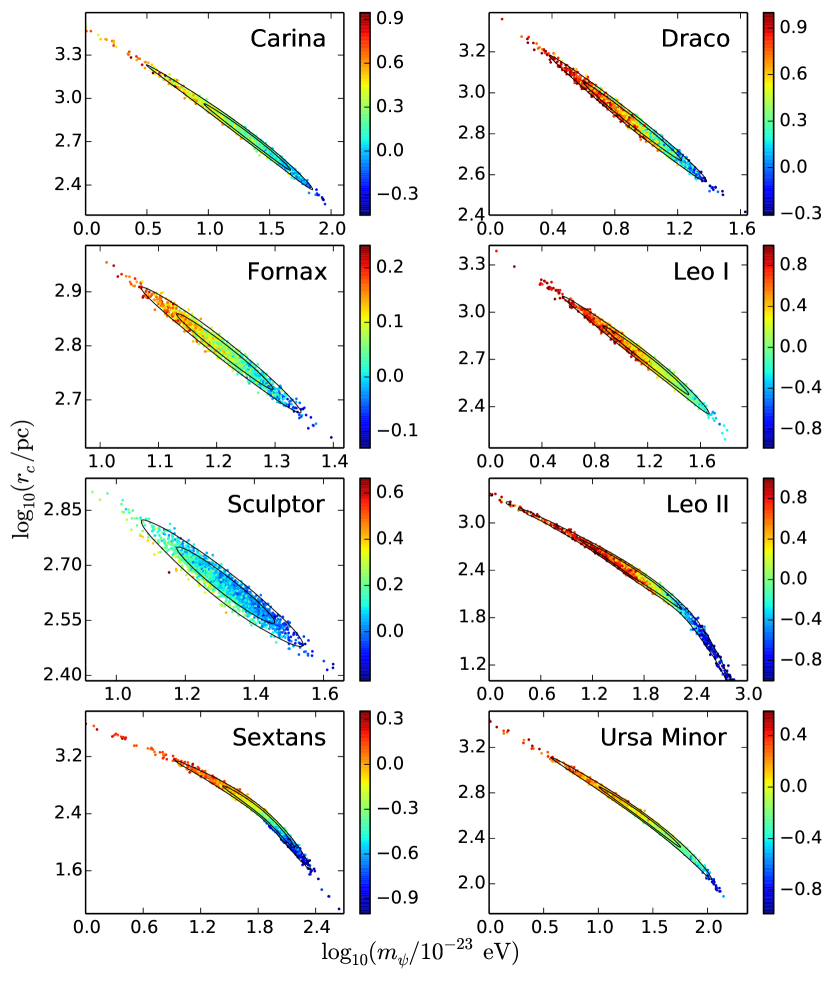
Table 1 lists the means, $1\sigma$, and $2\sigma$ confidence intervals of $r_{c}$, $m_{\psi}$, and $\beta$ for each dSph using the one-dimensional posterior distribution obtained from MCMC chains. We estimate the combined constraint by multiplying the one-dimensional posterior distributions of all dSphs based on the assumption that each dSph gives independent constraint on $m_{\psi}$. It leads to $1\sigma\,(2\sigma)$ confidence intervals of $m_{\psi}=1.79_{-0.17(-0.33)}^{+0.17(+0.35)}\times 10^{-22}\,\rm eV$ and a corresponding reduced chi-square of particle mass of $\chi_{\rm{red}}^{2}=1.2$. We also estimate the combined constraint by fitting all eight dSphs simultaneously, and the results are very consistent with the values given above. See Appendix B for details.

Note that the combined constraint is dominated by Fornax since it has the smallest variance among the eight dSphs. Also note that the anisotropy parameters $\beta$ of some dSphs have only $1\sigma$ constraints. We have adopted a larger range for the uniform prior of $\beta$ and also a different anisotropy prior distribution (see Section 4.1.3) and verified that the estimates of $m_{\psi}$ are consistent with Table 1.

Table 1: Constraints on model parameters from MCMC analysis. Values represent the means and $1\sigma$ ($2\sigma$) confidence intervals. The first and second rows for each dSph represent the results estimated from the kinematic data sets of W09 and W07, respectively. The anisotropy parameters of some dSphs have only $1\sigma$ constraints.

Galaxy	$\log_{10}[m_{\psi}/10^{-23}\rm{eV}]$	$\log_{10}[r_{c}/\rm{pc}]$	$-\log_{10}(1-\beta)$
Carina	$1.29^{+0.29(+0.50)}_{-0.18(-0.56)}$	$2.76^{+0.13(+0.35)}_{-0.18(-0.33)}$	$\hphantom{-}0.24^{+0.15(+0.35)}_{-0.18(-0.33)}$
	$1.09^{+0.18(+0.32)}_{-0.14(-0.35)}$	$2.87^{+0.09(+0.22)}_{-0.11(-0.21)}$	$\hphantom{-}0.29^{+0.10(+0.22)}_{-0.11(-0.20)}$
Draco	$0.91^{+0.20(+0.40)}_{-0.20(-0.40)}$	$2.86^{+0.12(+0.25)}_{-0.12(-0.24)}$	$\hphantom{-}0.53^{+0.35\hphantom{(+0.00)}}_{-0.24\hphantom{(-0.00)}}$
	$1.05^{+0.17(+0.31)}_{-0.15(-0.34)}$	$2.75^{+0.10(+0.21)}_{-0.10(-0.20)}$	$\hphantom{-}0.16^{+0.13(+0.31)}_{-0.16(-0.29)}$
Fornax	$1.21^{+0.06(+0.10)}_{-0.05(-0.11)}$	$2.79^{+0.05(+0.10)}_{-0.05(-0.09)}$	$\hphantom{-}0.07^{+0.06(+0.11)}_{-0.06(-0.11)}$
	$0.99^{+0.07(+0.13)}_{-0.07(-0.15)}$	$2.90^{+0.05(+0.11)}_{-0.05(-0.10)}$	$\hphantom{-}0.07^{+0.06(+0.12)}_{-0.06(-0.12)}$
Leo I	$1.18^{+0.25(+0.42)}_{-0.18(-0.46)}$	$2.71^{+0.13(+0.31)}_{-0.16(-0.29)}$	$\hphantom{-}0.33^{+0.22(+0.57)}_{-0.32(-0.48)}$
	$1.08^{+0.27(+0.44)}_{-0.17(-0.49)}$	$2.78^{+0.12(+0.31)}_{-0.17(-0.29)}$	$\hphantom{-}0.41^{+0.18(+0.50)}_{-0.28(-0.33)}$
Leo II	$1.71^{+0.39(+1.03)}_{-0.42(-0.85)}$	$2.30^{+0.37(+0.71)}_{-0.24(-0.94)}$	$\geq 0.21^{\hphantom{+0.00}\hphantom{(+0.00)}}_{\hphantom{+0.00}\hphantom{(+0.00)}}$
	$1.61^{+0.30(+0.64)}_{-0.29(-0.70)}$	$2.45^{+0.20(+0.45)}_{-0.21(-0.48)}$	$\hphantom{-}0.40^{+0.46\hphantom{(+0.00)}}_{-0.28\hphantom{(+0.00)}}$
Sculptor	$1.31^{+0.10(+0.18)}_{-0.08(-0.19)}$	$2.65^{+0.06(+0.14)}_{-0.07(-0.13)}$	$\hphantom{-}0.09^{+0.08(+0.18)}_{-0.09(-0.17)}$
	$1.11^{+0.14(+0.26)}_{-0.11(-0.26)}$	$2.77^{+0.08(+0.17)}_{-0.09(-0.17)}$	$\hphantom{-}0.22^{+0.10(+0.27)}_{-0.14(-0.25)}$
Sextans	$1.79^{+0.33(+0.53)}_{-0.19(-0.58)}$	$2.41^{+0.31(+0.61)}_{-0.30(-0.64)}$	$-0.31^{+0.39(+0.46)}_{-0.19(-0.63)}$
	$1.33^{+0.22(+0.38)}_{-0.13(-0.44)}$	$2.78^{+0.12(+0.35)}_{-0.17(-0.32)}$	$-0.12^{+0.13(+0.25)}_{-0.12(-0.26)}$
Ursa Minor	$1.39^{+0.29(+0.55)}_{-0.24(-0.65)}$	$2.59^{+0.18(+0.42)}_{-0.19(-0.44)}$	$-0.01^{+0.19(+0.39)}_{-0.14(-0.40)}$

Table 2: Summary of various stellar models applied to individual dSphs. The results generally agree with Table 1 and reveal insensitivity to these variations.

Galaxy	$\log_{10}[m_{\psi}/10^{-23}\rm{eV}]$	$\log_{10}[r_{c}/\rm{pc}]$	Description
Fornax	$1.09^{+0.07}_{-0.06}$	$2.85^{+0.05}_{-0.06}$	velocity dispersion (Amorisco and Evans 2012b)
	$1.15^{+0.07}_{-0.06}$	$2.84^{+0.05}_{-0.05}$	stellar density (generalized Plummer)
	$1.23^{+0.05}_{-0.07}$	$2.78^{+0.06}_{-0.05}$	soliton + NFW model
	$0.91^{+0.26}_{-0.09}$	$2.96^{+0.07}_{-0.19}$	stellar subpopulations
Leo I	$1.19^{+0.32}_{-0.20}$	$2.70^{+0.14}_{-0.20}$	velocity dispersion (tidal effect)
	$0.92^{+0.42}_{-0.21}$	$2.86^{+0.13}_{-0.24}$	stellar density (generalized Plummer)
Draco	$0.85^{+0.34}_{-0.19}$	$2.90^{+0.12}_{-0.19}$	stellar density (generalized Plummer)
Sextans	$0.51^{+0.23}_{-0.44}$	$3.31^{+0.25}_{-0.14}$	velocity dispersion (VLT)
	$1.64^{+0.48}_{-0.14}$	$2.55^{+0.24}_{-0.44}$	stellar density (exponential profile)
Carina	$1.41^{+0.44}_{-0.18}$	$2.67^{+0.14}_{-0.28}$	velocity dispersion (tidal effect)
Sculptor	$1.08^{+0.28}_{-0.22}$	$2.78^{+0.14}_{-0.14}$	stellar subpopulations (OM anisotropy)
	$1.21^{+0.17}_{-0.15}$	$2.70^{+0.10}_{-0.11}$	stellar subpopulations (constant anisotropy)

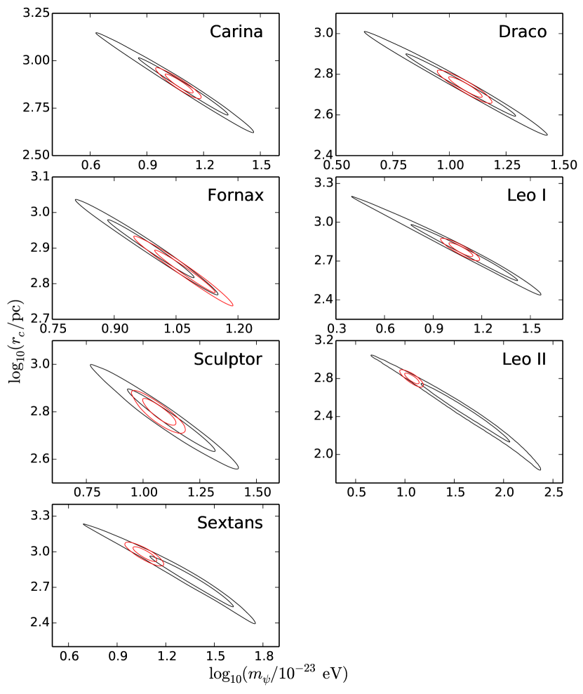
To further ascertain whether our estimate of $m_{\psi}$ is sensitive to the adopted observational data sets, we also apply the same Jeans analysis to the data of seven dSphs in Walker et al. (2007, hereafter W07), which does not include Ursa Minor. The results are shown in Figures 3 and 4. The reduced chi-square of the velocity dispersion fit of each dSph lies in the range $0.61\--1.66$. Note that the estimates of $m_{\psi}$ are, in general, lower than those obtained from W09, which arises from the generally higher velocity dispersions in W07. We address this discrepancy in more detail in Section 4.1.1. By multiplying the one-dimensional posterior distributions of the seven dSphs in W07, we get $1\sigma\,(2\sigma)$ confidence intervals of $m_{\psi}=1.18_{-0.13(-0.24)}^{+0.14(+0.28)}\times 10^{-22}\,\rm eV$ (see Appendix B for the results of fitting all dSphs in W07 simultaneously). This estimate is marginally consistent with the lower limit from W09. The corresponding reduced chi-square of particle mass is $\chi_{\rm{red}}^{2}=0.92$. The estimated means, $1\sigma$, and $2\sigma$ confidence intervals of $r_{c}$, $m_{\psi}$, and $\beta$ for each dSph are also listed in Table 1.

Figure 3: Same as Figure 1 but for the observational data set of Walker et al. (2007). The confidence intervals of the model parameters for each dSph are listed in Table 1.

Figure 4: Same as Figure 2 but for the observational data set of Walker et al. (2007). The confidence intervals of the model parameters for each dSph are listed in Table 1.

4 Discussion

4.1 Model Uncertainties

In order to consolidate the results of our Jeans analysis, we test how sensitive $m_{\psi}$ is to different models adopted in the MCMC calculations, including different observational data sets of the velocity dispersion profiles, different stellar density models, and a different orbital anisotropy prior distribution. Results are summarized in Table 2.

4.1.1 Velocity Dispersion

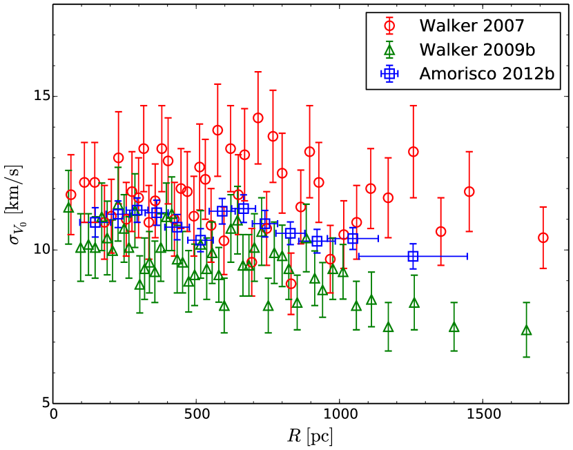
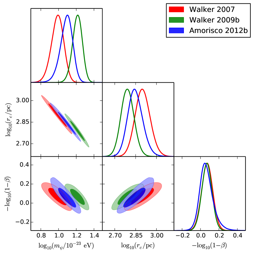
As shown in Table 1, the estimates of $m_{\psi}$ based on the velocity dispersion profiles of W07 are, in general, lower than those obtained from W09. It results from the generally higher velocity dispersions in W07. This difference is most significant in Fornax, where only about half of the data points in W07 and W09 overlap within the $1\sigma$ range (see Fig. 5). For comparison, we also show the velocity dispersion profile of Amorisco & Evans (2012b), which lies in between W07 and W09. The inverse-variance-weighted means of the velocity dispersions of Fornax in W07 and W09 are $\bar{\sigma}_{V_{0}}=11.6\pm 0.2$ and $\bar{\sigma}_{V_{0}}=9.4\pm 0.1$, respectively.

The lower velocity dispersion in W09 mainly results from a more restrictive selection of member stars, which only includes stars with a membership probability greater than $95\%$ (Walker et al., 2009b; Walker et al., 2009a). The discarded stars can have velocity $3\sigma$ away from the mean velocity (see Figure 1 and Table 1 in Walker et al. (2009a)), and thus discarding them would lower the velocity dispersion noticeably. Also, the new samples of Fornax in W09 lead to a gently declining velocity dispersion profile at large projected radii $(\geq 1\,\rm kpc)$ as compared with W07. Since Fornax provides the most stringent constraints on $m_{\psi}$, any difference in the observed velocity dispersion of Fornax would directly effect the estimate of $m_{\psi}$.

Figure 6 shows a comparison of the one-dimensional and two-dimensional posterior distributions of $m_{\psi}$, $r_{c}$, and $\beta$ from the three different velocity dispersion profiles of Fornax in Figure 5. It clearly shows that the estimate of $m_{\psi}$ is sensitive to the adopted velocity dispersion profile, where a lower and steeper profile leads to a higher estimate of $m_{\psi}$. The data sets of W07 and W09 thus likely bracket the uncertainty of the estimates of $m_{\psi}$, which lies in the range $m_{\psi}\sim 1\--2\times 10^{-22}\,\rm eV$. We emphasize that this value is in good agreement with other independent estimates from the stellar subpopulations in dSphs (Schive et al., 2014a; Marsh & Pop, 2015), the high-redshift luminosity functions (Bozek et al., 2015; Schive et al., 2016; Corasaniti et al., 2016), and the Thomson optical depth to the cosmic microwave background (Bozek et al., 2015; Schive et al., 2016).

Figure 5: Comparison of the projected velocity dispersion profiles of Fornax given by Walker et al. (2007) (circles), Walker et al. (2009b) (triangles), and Amorisco & Evans (2012b) (squares).

Figure 6: Posterior distributions of $m_{\psi}$, $r_{c}$, and $\beta$ in our MCMC analysis for the three different velocity dispersion data sets of Fornax shown in Figure 5. Solid curves in the diagonal panels show the one-dimensional marginalized distributions. Filled contours in the corner panels show the $1\sigma$ and $2\sigma$ confidence regions.

We also notice that the estimate of $m_{\psi}$ from Sextans in W09 is higher than those obtained from other dSphs in both W07 and W09. For example, by using the data of Sextans in W07, we find a $1\sigma$ confidence interval of $\log_{10}[m_{\psi}/10^{-23}\rm{eV}]=1.33_{-0.13}^{+0.22}$, significantly lower than the value determined using W09 but more consistent with other dSphs (see Table 1). It is mainly because the inverse-variance-weighted mean of the velocity dispersion of W07 is $\bar{\sigma}_{V_{0}}=7.1\pm 0.3$, apparently higher than that of W09, $\bar{\sigma}_{V_{0}}=6.1\pm 0.3$.

To look into this discrepancy, we further apply the same MCMC algorithm to the more recent Very Large Telescope (VLT) observation of Sextans (Battaglia et al., 2011), which is in better agreement with W07 than W09. We find $r_{c}\sim 1.5-3.5\,\rm kpc$, consistent with Battaglia et al. (2011) using a pseudo-isothermal model for the dark matter density profile. However, we get $\log_{10}[m_{\psi}/10^{-23}\rm{eV}]=0.51_{-0.44}^{+0.23}$ in a $1\sigma$ confidence interval, apparently lower than the estimates from both W07 and W09. The inconsistency between $m_{\psi}$ determined from the three different observations therefore suggest that the current data of Sextans provide a poor constraint on $m_{\psi}$.

One caveat about the VLT data is that they extend to as far as $\sim 2.5\,\rm kpc$, which lies beyond $3\,r_{c}$ for the $r_{c}$ estimated from W07. It thus seems reasonable to consider an NFW halo outside the central soliton. However, the NFW halo introduces two additional free parameters, making the Jeans analysis infeasible due to the very few data points.

There is evidence of tidal stripping in the outermost parts of both Carina and Leo I (Muñoz et al., 2006; Mateo et al., 2008; Battaglia et al., 2012). Therefore, for these two dSphs we also apply Jeans analysis discarding the outermost one data point in the velocity dispersions. We obtain $1\sigma$ confidence intervals of $\log_{10}[m_{\psi}/10^{-23}\rm{eV}]=1.41_{-0.18}^{+0.44}$ for Carina and $\log_{10}[m_{\psi}/10^{-23}\rm{eV}]=1.19_{-0.20}^{+0.32}$ for Leo I, both consistent with Table 1. However, we notice the relatively larger ranges in the revised estimates of $m_{\psi}$, which arise from the $m_{\psi}\--r_{c}$ degeneracy. For example, for Carina the outermost data point has a projected radius of $R\sim 870\,\rm pc$, well beyond the estimated mean core radius, $r_{c}=570\,\rm pc$. For comparison, the second outermost data point has a projected radius of $R\sim 530\,\rm pc$, comparable to the core radius. Therefore, the outermost data point is important for constraining the dark matter mass profile and breaking the $m_{\psi}\--r_{c}$ degeneracy.

4.1.2 Stellar Density

It is important to investigate the impact of different stellar density models. First, in addition to having $R_{h}$ randomly sampled from a Gaussian distribution with a given mean and variance, we also experiment with fixing $R_{h}$ to the mean value and validate that the estimates of $m_{\psi}$ are largely unchanged in all dSphs. Second, we adopt a generalized Plummer model (Mashchenko, 2015), $I(R)=L_{0}\left[1+(R/b)^{2}\right]^{-(\alpha-1)/2}$, where $L_{0}$ is the central luminosity, $b$ is the core radius, and $\alpha$ is an integer which must be greater than three for a finite total stellar mass. The standard Plummer model corresponds to $\alpha=5$. This model has been shown to fit well with recent observations of Fornax (Coleman et al., 2005), Leo I (Smolčić et al., 2007), and Draco (Odenkirchen et al., 2001) even at the tidal radius. The corresponding estimates of particle mass are $\log_{10}[m_{\psi}/10^{-23}\rm{eV}]=1.15_{-0.06}^{+0.07}$ for Fornax, $\log_{10}[m_{\psi}/10^{-23}\rm{eV}]=0.92_{-0.21}^{+0.42}$ for Leo I, and $\log_{10}[m_{\psi}/10^{-23}\rm{eV}]=0.85_{-0.19}^{+0.34}$ for Draco, in good agreement with Table 1. A relatively larger difference is found in Leo I. It is because the data of (Smolčić et al., 2007), when fitted with a King profile, suggests a $50\%$ larger King core radius but a similar tidal radius compared to the data of Irwin & Hatzidimitriou (1995). Finally, for Sextans, we also apply an exponential profile (Irwin & Hatzidimitriou, 1995). It leads to $\log_{10}[m_{\psi}/10^{-23}\rm{eV}]=1.64_{-0.14}^{+0.48}$, consistent with Table 1.

4.1.3 Orbital Anisotropy

For the orbital anisotropy, we investigate this issue with a different uniform prior, $\eta=(\bar{v_{r}^{2}}-\bar{v_{\theta}^{2}})/(\bar{v_{r}^{2}}+\bar{v_{\theta}^{2}})$ (Mashchenko et al., 2006). This form has the advantage of being symmetric for tangential and radial anisotropies, where $\eta=-1$ for pure tangential orbit, $\eta=0$ for isotropic orbit, and $\eta=1$ for pure radial orbit. We validate that the resulting $m_{\psi}$ is very consistent with Table 1.

One caveat in Jeans analysis is that the choice of functional form for stellar anisotropy may affect the estimate of enclosed mass due to the mass-anisotropy degeneracy (e.g., Gonzáles-Morales et al., 2016). Using more flexible dynamical modeling methods that extract more information from the line-of-sight velocity or stellar distributions, such as modeling higher moments (Łokas, 2002), phase-space analyses (Kleyna et al., 2002; Amorisco & Evans, 2012a), and Schwarzschild’s orbit superposition methods (Jardel & Gebhardt, 2012; Breddels et al., 2013), can help reduce the degeneracy and provide a more robust constraint on $m_{\psi}$. We plan to address this issue in the future.

4.2 Soliton + NFW model

To justify the assumption that all stars are located within the central soliton core, we investigate the case where the soliton core connects to an NFW halo at a larger radius. The overall density profile, as shown by Schive et al. (2014a); Schive et al. (2014b); Marsh & Pop (2015), can be modeled as

$$\rho(r)=\Theta(r_{\epsilon}-r)\rho_{\rm{soliton}}(r)+\Theta(r-r_{\epsilon})\rho_{\rm{NFW}},$$ (6)

where

$$\rho_{\rm{NFW}}(r)=\frac{\rho_{0}}{(\frac{r}{r_{s}})(1+\frac{r}{r_{s}})^{2}}$$ (7)

is the NFW profile, $\rho_{\rm{soliton}}(r)$ is given in Equation (4), $\Theta(r)$ is a step function, and $r_{\epsilon}$ is the transition radius between soliton and NFW halo given by $\rho_{\rm{NFW}}(r_{\epsilon})=\rho_{\rm{soliton}}(r_{\epsilon})=\epsilon\rho_{\rm{soliton}}(0)$. Since $\rho_{0}$ can be uniquely determined from a given $r_{\epsilon}$ and $r_{s}$, this model introduces two additional free parameters, $\left\{\log_{10}\epsilon,\log_{10}[r_{s}/\rm{pc}]\right\}$, which we model with uniform priors over the ranges $-5\leq\log_{10}\epsilon\leq\log_{10}0.5$ and $1\leq\log_{10}[r_{s}/\rm{pc}]\leq 4$.

Note that the soliton core mass $(M_{c})$ has been found to correlate with halo virial mass $(M_{h})$ in the mass range $\sim 10^{8}\--5\times 10^{11}\,M_{\sun}$ (Schive et al., 2014b) as $M_{c}=0.25(M_{h}/M_{\rm{min},0})^{1/3}M_{\rm{min},0}$, where $M_{\rm{min},0}\sim 4.4\times 10^{7}(m_{\psi}/10^{-22}\,\rm eV)^{-3/2}\,M_{\sun}$ is the predicted minimum $\psi{\rm DM}$ halo mass at the present day. Using this relation can, in principle, eliminate one free parameter. However, it is unclear whether this relation, which is determined from isolated galaxies, can be applied to satellite dSph galaxies underwent complex evolution history. In order to make our analysis more robust, we thus do not take this core-halo mass relation into account when conducting Jeans analysis.

We apply this soliton + NFW model to Fornax since it provides the strongest constraint on $m_{\psi}$ and has around half of the observation points lying outside the core radius determined from the soliton-only model. To properly constrain the central soliton density profile that has two free parameters, we set the lower limit of $r_{c}$ to the position of the second innermost observation point, which is $\sim 100\,\rm pc$. This is a very weak constraint since the core size of Fornax is typically found to be $\sim 1\,\rm kpc$ (e.g., Amorisco et al., 2013; Walker & Peñarrubia, 2011). We obtain $\log_{10}[m_{\psi}/10^{-23}\rm{eV}]=1.23_{-0.07(-0.14)}^{+0.05(+0.13)}$, and $\log_{10}[r_{c}/\rm{pc}]=2.78_{-0.05(-0.11)}^{+0.06(+0.11)}$ (also listed in Table 2), consistent with the soliton-only model (see Table 1). The transition radius between soliton and NFW halo is found to be greater than $\sim 2.5\,r_{c}$, where the soliton density has dropped by a factor of 30. The scale radius $r_{s}$ is unconstrained, which is expected since most stars still reside within the transition radius. The slightly larger $m_{\psi}$ and smaller $r_{c}$ arise from the additional gravity support from the external NFW halo for stars outside the transition radius.

4.3 Stellar Subpopulations

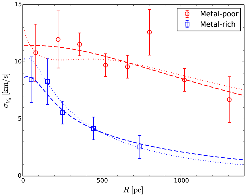
Several dSphs have been found to exhibit more than one stellar subpopulations, each with different metallicity and kinematics. Modeling different subpopulations separately in the same gravitational potential can further break the mass-anisotropy degeneracy in the Jeans analysis (Battaglia et al., 2008). We model the stellar density and velocity dispersion profiles of the metal-rich (MR) and metal-poor (MP) subpopulations in Sculptor (Battaglia et al., 2008). The MR subpopulation is known to be better described by radially biased orbits in the outer region due to its rapidly declining velocity dispersion profile (Battaglia et al., 2008; Strigari et al., 2014). Therefore, we follow Battaglia et al. (2008) and adopt the Osipkov-Merritt (OM, Osipkov, 1979; Merritt, 1985) anisotropy profile on the MR subpopulation, and use either constant or OM anisotropy on the MP subpopulation. The OM anisotropy profile is given by $\beta(r)=r^{2}/(r^{2}+r_{a}^{2})$, where $r_{a}$ is the anisotropy radius with $\beta\rightarrow 0$ for $r\ll r_{a}$ and $\beta\rightarrow 1$ for $r\gg r_{a}$. We discard the last observation data point of the MP subpopulation because of its large uncertainty. The $1\sigma$ ranges for constant and OM anisotropy on the MP subpopulation are $\log_{10}[m_{\psi}/10^{-23}\rm{eV}]=1.21_{-0.15}^{+0.17}$ and $\log_{10}[m_{\psi}/10^{-23}\rm{eV}]=1.08_{-0.22}^{+0.28}$, respectively (also listed in Table 2). Both are in good agreement with Table 1. The empirical and the best-fit velocity dispersion profiles in our MCMC chains are shown in Figure 7, which have chi-squares of $\chi^{2}=6.8$ (with $\chi_{\rm{MP}}^{2}=5.4,\,\chi_{\rm{MR}}^{2}=1.4$) and $\chi^{2}=4.3$ (with $\chi_{\rm{MP}}^{2}=3.8,\,\chi_{\rm{MR}}^{2}=0.5$) for constant and OM anisotropy on the MP subpopulation, respectively.

Figure 7: Projected velocity dispersion profiles of the two stellar subpopulations in Sculptor. Error bars show the observational $1\sigma$ uncertainties (Battaglia et al., 2008). Dashed (dotted) lines show the best-fit $\psi{\rm DM}$ model in the hypothesis of OM (constant) anisotropy profile on the MP subpopulation and OM anisotropy profile on the MR subpopulation.

Fornax also has three distinct stellar subpopulations (Amorisco & Evans, 2012c). The intrinsic rotation detected in the MP and intermediate-metallicity (IM) subpopulations is ${\Omega}_{int}\sim 1-2\,\rm km\,s^{-1}\,\rm kpc^{-1}$, which is negligible compared with velocity dispersion. For example, at the outermost kinematic data point ($\sim 1\,\rm kpc$), the ratio between rotation velocity and velocity dispersion is only $\sim 0.3$ (Amorisco & Evans, 2012c). Therefore, we neglect rotation and apply Jeans analysis to the three subpopulations using the stellar density and velocity dispersion profiles in Amorisco et al. (2013).

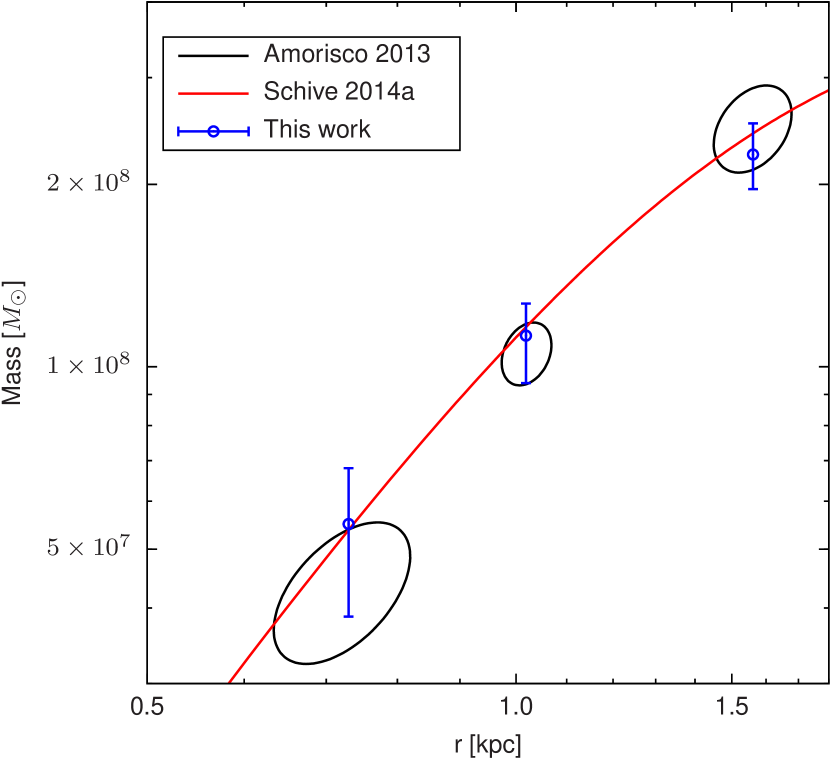
Note that Amorisco et al. (2013) applied an empirical relation between $M(<1.67R_{h})$, $R_{h}$, and $\bar{\sigma}_{V_{0}}$ to the three subpopulations of Fornax to estimate the total mass profile (contours in Figure 9). This empirical mass estimator has been derived to describe a wide family of models based on the Michie-King phase-space distribution function (Amorisco & Evans, 2012a), where velocity distribution is isotropic in the center and nearly radial in the outer region, similar to the OM anisotropy model. Therefore, in order to compare with their result, we adopt OM anisotropy profiles on all three stellar subpopulations. In addition, since the kinematic data have observational uncertainties in both $\sigma_{V_{0}}(R_{i})$ and $R_{i}$, we follow Ma et al. (2013) and convert the uncertainty associated with $R_{i}$ into an effective variance in $\sigma_{V_{0}}(R_{i})$ as $\rm{Var}[\sigma_{V_{0}}(R_{i})]+{\sigma}^{\prime}_{p}(R_{i})\rm{Var}[R_{i}]$, where ${\sigma}^{\prime}_{p}(R_{i})$ is the derivative of the estimated velocity dispersions.

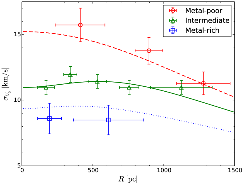
We obtain $1\sigma$ confidence intervals of $\log_{10}[m_{\psi}/10^{-23}\rm{eV}]=0.91_{-0.09}^{+0.26}$ and $\log_{10}[r_{c}/\rm{pc}]=2.96_{-0.19}^{+0.07}$. Figure 8 shows the empirical velocity dispersions of the three subpopulations and our estimated velocity dispersions, which correspond to the maximum likelihood point within the $1\sigma$ range. Figure 9 shows the corresponding $1\sigma$ total enclosed mass, $M(<1.67R_{h})$, where $R_{h}$ is the half-light radius of each subpopulation. This result is in good agreement with the $1\sigma$ estimate of Amorisco et al. (2013, contours in Figure 9) It is also consistent with the estimate of Schive et al. (2014a, solid line in the figure) using only the IM subpopulation, which gives $m_{\psi}=8.1_{-1.7}^{+1.6}\times 10^{-23}\,\rm eV$ and $r_{c}=0.92_{-0.11}^{+0.15}\,\rm kpc$

Note that we find another local maximum of likelihood function around $\log_{10}[m_{\psi}/10^{-23}\rm{eV}]=0.59_{-0.15}^{+0.18}$ and $\log_{10}[r_{c}/\rm{pc}]=3.18_{-0.11}^{+0.10}$, with anisotropy radii of the IM and MP subpopulations close to their $R_{h}$. However, this local peak only covers a small volume in the five-dimensional posterior distributions and is negligible in the one-dimensional marginalized distributions of $m_{\psi}$ and $r_{c}$. Also note that the MR subpopulation, which has the lowest velocity dispersion, has only two observation points and thus gives a relatively weak constraint compared with the IM and MP subpopulations. Accordingly, the estimate of $m_{\psi}$ is more consistent with that using W07, which has a higher velocity dispersion closer to IM and MP than to MR.

Figure 8: Projected velocity dispersion profiles of the three stellar subpopulations in Fornax. Error bars show the observational $1\sigma$ uncertainties (Amorisco et al., 2013), and lines show the best-fit profiles within the $1\sigma$ ranges of our estimated $m_{\psi}$ and $r_{c}$ based on the soliton density profile in $\psi{\rm DM}$.

Figure 9: Total enclosed mass estimated from the three stellar subpopulations shown in Figure 8. Error bars represent the $1\sigma$ confidence intervals estimated in this work. For comparison, solid contours show the $1\sigma$ estimate of Amorisco et al. (2013), and solid line shows the best-fit soliton model using only the intermediate-metallicity subpopulation Schive et al. (2014a). These results are in good agreement with each other.

5 Conclusion

Wave dark matter ($\psi{\rm DM}$), characterized by a single parameter, the dark matter particle mass $m_{\psi}$, predicts a central soliton core in every galaxy. In this work, we have applied the Jeans equation to the empirical velocity dispersion profiles of eight classical dSphs in the Milky Way so as to constrain $m_{\psi}$. We find combined $1\sigma(2\sigma)$ confidence intervals of $m_{\psi}=1.18_{-0.13(-0.24)}^{+0.14(+0.28)}\times 10^{-22}\,\rm eV$ and $m_{\psi}=1.79_{-0.17(-0.33)}^{+0.17(+0.35)}\times 10^{-22}\,\rm eV$ using the observational data sets of Walker et al. (2007) and Walker et al. (2009b), respectively. The discrepancy of W07 and W09 suggests that a more elaborate star membership determination for calculating velocity dispersion will improve the constraint on $m_{\psi}$ further.

This combined constraint of $m_{\psi}$ is dominated by Fornax but is consistent with the estimate from individual dSphs. It is also in good agreement with other independent constraints from, for instance, the stellar subpopulations in dSphs (Schive et al., 2014a; Marsh & Pop, 2015), the high-redshift luminosity functions (Bozek et al., 2015; Schive et al., 2016), and the Thomson optical depth to CMB (Bozek et al., 2015; Schive et al., 2016), which all suggest $m_{\psi}\sim 10^{-22}\,\rm eV$.

To consolidate the results, we have investigated a variety of models in the MCMC calculations, including different velocity dispersion data, stellar density profiles, and orbital anisotropy priors. We have also extended the soliton-only model to account for an NFW halo at a larger radius, and further considered distinct stellar subpopulations in both Sculptor and Fornax. It is demonstrated that these factors have only minor effect on the estimate of $m_{\psi}$.

Finally, we emphasize that the existence of large cores in dSphs is still under debate (e.g., Strigari et al., 2010). The methodology of our study is to assume a soliton core profile, Equation (4), and ascertain whether the resulting constraint on $m_{\psi}$ is consistent with other independent constraints mentioned above. In other words, we focus on validating the self-consistency of $\psi{\rm DM}$, but not on falsifying the NFW profile or the CDM model. In principle, the latter can be addressed by extending the soliton + NFW model to allow for a much smaller soliton component and we plan to explore it in the future.

6 Acknowledgement

This work is supported in part by the National Science Council of Taiwan under the grant MOST 103-2112-M-002-020-MY3.

Appendix A Soliton Mass Profile

The soliton mass profile can be explicitly derived from Equation (4) as

$$M_{\rm{soliton}}(r)=\frac{4.2\times 10^{9}\,M_{\sun}}{(m_{\psi}/10^{-23}\,\rm eV)^{2}(r_{c}/\,\rm pc)}\frac{1}{(a^{2}+1)^{7}}\\ (3465a^{13}+23100a^{11}+65373a^{9}+101376a^{7}+92323a^{5}\\ +48580a^{3}-3465a+3465(a^{2}+1)^{7}\arctan{(a)}),$$ (8)

where $a=(2^{1/8}-1)^{1/2}(r/r_{c})$.

Appendix B Joint analysis

To consolidate our estimates of $m_{\psi}$, here we perform the joint analysis by fitting all dSphs simultaneously. Assuming all dSphs are independent data sets, the joint likelihood function is the product of the likelihood functions of individual dSphs. We treat the particle mass $m_{\psi}$ as a global parameter shared by all dSphs, while allow $r_{c}$, $\beta$ to vary in different dSphs. To account for the uncertainty in $R_{h}$, we adopt Gaussian priors with means and standard deviations equal to the observations, and then integrate it out when calculating the posterior distributions of other model parameters.

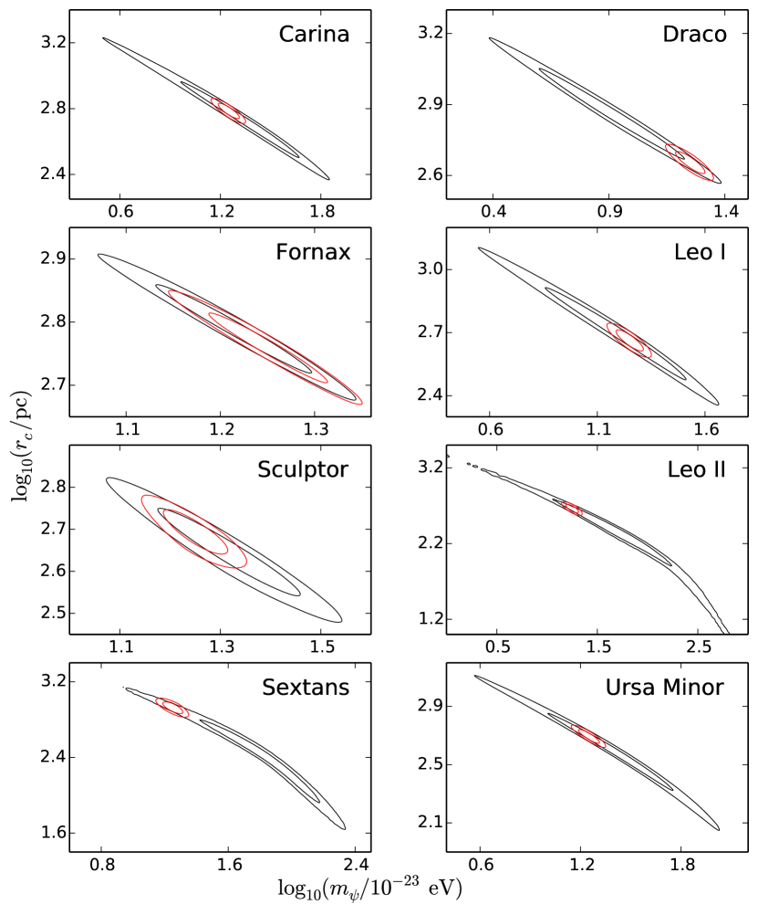
Figures 10 and 11 show the $m_{\psi}$-$r_{c}$ confidence contours from the joint analysis, overplotted with the previous results shown in Figures 2 and 4 obtained from individual dSphs. The $1\sigma\,(2\sigma)$ confidence intervals of $m_{\psi}$ is $1.79_{-0.17(-0.33)}^{+0.17(+0.35)}\times 10^{-22}\,\rm eV$ from the W09 data sets and $1.18_{-0.13(-0.25)}^{+0.13(+0.28)}\times 10^{-22}\,\rm eV$ from the W07 data sets. These constraints are in good agreement with the estimates given in Section 3 where different dSphs are fitted separately.

Figure 10: Posterior distributions of $m_{\psi}$ and $r_{c}$ obtained from the joint analysis (red lines), overplotted with Figure 2 obtained from analyzing individual dSphs separately (black lines). Contours show the $1\sigma$ and $2\sigma$ confidence regions.

Figure 11: Same as Figure 10 but for the observational data set of Walker et al. (2007).

References

- Amorisco & Evans (2012a) Amorisco N. C., Evans N. W., 2012a, MNRAS, 419, 184
- Amorisco & Evans (2012b) Amorisco N. C., Evans N. W., 2012b, MNRAS, 424, 1899
- Amorisco & Evans (2012c) Amorisco N. C., Evans N. W., 2012c, ApJ, 756, L2
- Amorisco et al. (2013) Amorisco N. C., Agnello A., Evans N. W., 2013, MNRAS, 429, L89
- An et al. (1998) An L., Brooks S., Gelman A., 1998, Journal of Computational and Graphical Statistics, 7, 434
- Arraki et al. (2014) Arraki K. S., Klypin A., More S., Trujillo-Gomez S., 2014, MNRAS, 438, 1466
- Arvanitaki et al. (2010) Arvanitaki A., Dimopoulos S., Dubovsky S., Kaloper N., March-Russell J., 2010, Phys. Rev. D, 81, 123530
- Battaglia et al. (2008) Battaglia G., Helmi A., Tolstoy E., Irwin M., Hill V., Jablonka P., 2008, ApJ, 681, L13
- Battaglia et al. (2011) Battaglia G., Tolstoy E., Helmi A., Irwin M., Parisi P., Hill V., Jablonka P., 2011, MNRAS, 411, 1013
- Battaglia et al. (2012) Battaglia G., Irwin M., Tolstoy E., de Boer T., Mateo M., 2012, ApJ, 761, L31
- Battaglia et al. (2013) Battaglia G., Helmi A., Breddels M., 2013, New Astron. Rev., 57, 52
- Bennett et al. (2013) Bennett C. L., et al., 2013, ApJS, 208, 20
- Benson et al. (2002) Benson A. J., Lacey C. G., Baugh C. M., Cole S., Frenk C. S., 2002, MNRAS, 333, 156
- Binney & Tremaine (2008) Binney J., Tremaine S., 2008, Galactic Dynamics. Princeton Univ. Press, Princeton
- Böhmer & Harko (2007) Böhmer C. G., Harko T., 2007, J. Cosmology Astropart. Phys., 6, 025
- Borriello & Salucci (2001) Borriello A., Salucci P., 2001, MNRAS, 323, 285
- Boylan-Kolchin et al. (2011) Boylan-Kolchin M., Bullock J. S., Kaplinghat M., 2011, MNRAS, 415, L40
- Boylan-Kolchin et al. (2012) Boylan-Kolchin M., Bullock J. S., Kaplinghat M., 2012, MNRAS, 422, 1203
- Bozek et al. (2015) Bozek B., Marsh D. J. E., Silk J., Wyse R. F. G., 2015, MNRAS, 450, 209
- Breddels et al. (2013) Breddels M. A., Helmi A., van den Bosch R. C. E., van de Ven G., Battaglia G., 2013, MNRAS, 433, 3173
- Brooks et al. (2013) Brooks A. M., Kuhlen M., Zolotov A., Hooper D., 2013, ApJ, 765, 22
- Bullock et al. (2000) Bullock J. S., Kravtsov A. V., Weinberg D. H., 2000, ApJ, 539, 517
- Burkert (1995) Burkert A., 1995, ApJ, 447, L25
- Calabrese & Spergel (2016) Calabrese E., Spergel D. N., 2016, preprint (arXiv:1603.07321)
- Chavanis (2011) Chavanis P.-H., 2011, Phys. Rev. D, 84, 043531
- Chiueh (2014) Chiueh T., 2014, arXiv:1409.0380
- Cole et al. (2005) Cole S., et al., 2005, MNRAS, 362, 505
- Coleman et al. (2005) Coleman M. G., Da Costa G. S., Bland-Hawthorn J., Freeman K. C., 2005, AJ, 129, 1443
- Colín et al. (2000) Colín P., Avila-Reese V., Valenzuela O., 2000, ApJ, 542, 622
- Corasaniti et al. (2016) Corasaniti P. S., Agarwal S., Marsh D. J. E., Das S., 2016, preprint (arXiv:1611.05892)
- Davidson (2015) Davidson S., 2015, Astroparticle Physics, 65, 101
- El-Zant et al. (2001) El-Zant A., Shlosman I., Hoffman Y., 2001, ApJ, 560, 636
- Flores & Primack (1994) Flores R. A., Primack J. R., 1994, ApJ, 427, L1
- Frenk & White (2012) Frenk C. S., White S. D. M., 2012, Annalen der Physik, 524, 507
- Goerdt et al. (2006) Goerdt T., Moore B., Read J. I., Stadel J., Zemp M., 2006, MNRAS, 368, 1073
- Gonzáles-Morales et al. (2016) Gonzáles-Morales A. X., Marsh D. J. E., Peñarrubia J., Ureña-López L., 2016, preprint (arXiv:1609.05856)
- Goodman (2000) Goodman J., 2000, New Astron., 5, 103
- Governato et al. (2010) Governato F., et al., 2010, Nature, 463, 203
- Governato et al. (2012) Governato F., et al., 2012, MNRAS, 422, 1231
- Guth et al. (2015) Guth A. H., Hertzberg M. P., Prescod-Weinstein C., 2015, Phys. Rev. D, 92, 103513
- Guzmán & Matos (2000) Guzmán F. S., Matos T., 2000, Classical and Quantum Gravity, 17, L9
- Hastings (1970) Hastings W., 1970, Biometrika, 57, 97
- Hlozek et al. (2015) Hlozek R., Grin D., Marsh D. J. E., Ferreira P. G., 2015, Phys. Rev. D, 91, 103512
- Hu et al. (2000) Hu W., Barkana R., Gruzinov A., 2000, Physical Review Letters, 85, 1158
- Irwin & Hatzidimitriou (1995) Irwin M., Hatzidimitriou D., 1995, MNRAS, 277, 1354
- Jardel & Gebhardt (2012) Jardel J. R., Gebhardt K., 2012, ApJ, 746, 89
- Jardel & Gebhardt (2013) Jardel J. R., Gebhardt K., 2013, ApJ, 775, L30
- Khlopov et al. (1985) Khlopov M. I., Malomed B. A., Zeldovich I. B., 1985, MNRAS, 215, 575
- Kleyna et al. (2002) Kleyna J., Wilkinson M. I., Evans N. W., Gilmore G., Frayn C., 2002, MNRAS, 330, 792
- Kleyna et al. (2003) Kleyna J. T., Wilkinson M. I., Gilmore G., Evans N. W., 2003, ApJ, 588, L21
- Kleyna et al. (2005) Kleyna J. T., Wilkinson M. I., Evans N. W., Gilmore G., 2005, ApJ, 630, L141
- Klypin et al. (1999) Klypin A., Kravtsov A. V., Valenzuela O., Prada F., 1999, ApJ, 522, 82
- Lewis & Bridle (2002) Lewis A., Bridle S., 2002, Phys. Rev., D66, 103511
- Lewis et al. (2000) Lewis A., Challinor A., Lasenby A., 2000, Astrophys. J., 538, 473
- Łokas (2002) Łokas E. L., 2002, MNRAS, 333, 697
- Łokas & Mamon (2003) Łokas E. L., Mamon G. A., 2003, MNRAS, 343, 401
- Lora & Magaña (2014) Lora V., Magaña J., 2014, J. Cosmology Astropart. Phys., 9, 011
- Lora et al. (2012) Lora V., Magaña J., Bernal A., Sánchez-Salcedo F. J., Grebel E. K., 2012, J. Cosmology Astropart. Phys., 2, 011
- Lovell et al. (2012) Lovell M. R., et al., 2012, MNRAS, 420, 2318
- Ma et al. (2013) Ma Y.-Z., Hinshaw G., Scott D., 2013, ApJ, 771, 137
- Macciò et al. (2012) Macciò A. V., Paduroiu S., Anderhalden D., Schneider A., Moore B., 2012, MNRAS, 424, 1105
- Marsh (2015) Marsh D. J. E., 2015, preprint (arXiv:1510.07633)
- Marsh & Ferreira (2010) Marsh D. J. E., Ferreira P. G., 2010, Phys. Rev. D, 82, 103528
- Marsh & Pop (2015) Marsh D. J. E., Pop A.-R., 2015, MNRAS, 451, 2479
- Marsh & Silk (2014) Marsh D. J. E., Silk J., 2014, MNRAS, 437, 2652
- Mashchenko (2015) Mashchenko S., 2015, preprint (arXiv:1504.08273)
- Mashchenko et al. (2006) Mashchenko S., Sills A., Couchman H. M., 2006, ApJ, 640, 252
- Mashchenko et al. (2008) Mashchenko S., Wadsley J., Couchman H. M. P., 2008, Science, 319, 174
- Mateo (1998) Mateo M. L., 1998, ARA&A, 36, 435
- Mateo et al. (2008) Mateo M., Olszewski E. W., Walker M. G., 2008, ApJ, 675, 201
- Matos et al. (2000) Matos T., Guzmán F. S., Ureña-López L. A., 2000, Classical and Quantum Gravity, 17, 1707
- Merritt (1985) Merritt D., 1985, MNRAS, 214, 25P
- Metropolis et al. (1953) Metropolis N., Rosenbluth A. W., Rosenbluth M. N., Teller A. H., Teller E., 1953, J. Chem. Phys., 21, 1087
- Moore (1994) Moore B., 1994, Nature, 370, 629
- Moore et al. (1999) Moore B., Ghigna S., Governato F., Lake G., Quinn T., Stadel J., Tozzi P., 1999, ApJ, 524, L19
- Muñoz et al. (2006) Muñoz R. R., et al., 2006, ApJ, 649, 201
- Navarro et al. (1996) Navarro J. F., Eke V. R., Frenk C. S., 1996, MNRAS, 283, L72
- Navarro et al. (1997) Navarro J. F., Frenk C. S., White S. D. M., 1997, ApJ, 490, 493
- Odenkirchen et al. (2001) Odenkirchen M., et al., 2001, AJ, 122, 2538
- Oh et al. (2008) Oh S.-H., de Blok W. J. G., Walter F., Brinks E., Kennicutt Jr. R. C., 2008, AJ, 136, 2761
- Osipkov (1979) Osipkov L. P., 1979, Soviet Astronomy Letters, 5, 42
- Peebles (2000) Peebles P. J. E., 2000, ApJ, 534, L127
- Pfrommer et al. (2012) Pfrommer C., Chang P., Broderick A. E., 2012, ApJ, 752, 24
- Planck Collaboration et al. (2015) Planck Collaboration et al., 2015, preprint (arXiv:1502.01589)
- Pontzen & Governato (2014) Pontzen A., Governato F., 2014, Nature, 506, 171
- Read & Gilmore (2005) Read J. I., Gilmore G., 2005, MNRAS, 356, 107
- Robles & Matos (2013) Robles V. H., Matos T., 2013, ApJ, 763, 19
- Sahni & Wang (2000) Sahni V., Wang L., 2000, Phys. Rev. D, 62, 103517
- Salucci et al. (2012) Salucci P., Wilkinson M. I., Walker M. G., Gilmore G. F., Grebel E. K., Koch A., Frigerio Martins C., Wyse R. F. G., 2012, MNRAS, 420, 2034
- Sánchez-Salcedo et al. (2006) Sánchez-Salcedo F. J., Reyes-Iturbide J., Hernandez X., 2006, MNRAS, 370, 1829
- Sarkar et al. (2016) Sarkar A., Mondal R., Das S., Sethi S. K., Bharadwaj S., Marsh D. J. E., 2016, J. Cosmology Astropart. Phys., 4, 012
- Schive et al. (2014a) Schive H.-Y., Chiueh T., Broadhurst T., 2014a, Nat. Phys., 10, 496
- Schive et al. (2014b) Schive H.-Y., Liao M.-H., Woo T.-P., Wong S.-K., Chiueh T., Broadhurst T., Hwang W.-Y. P., 2014b, Phys. Rev. Lett., 113, 261302
- Schive et al. (2016) Schive H.-Y., Chiueh T., Broadhurst T., Huang K.-W., 2016, ApJ, 818, 89
- Sikivie & Yang (2009) Sikivie P., Yang Q., 2009, Physical Review Letters, 103, 111301
- Sin (1994) Sin S.-J., 1994, Phys. Rev. D, 50, 3650
- Smecker-Hane et al. (1994) Smecker-Hane T. A., Stetson P. B., Hesser J. E., Lehnert M. D., 1994, AJ, 108, 507
- Smolčić et al. (2007) Smolčić V., Zucker D. B., Bell E. F., Coleman M. G., Rix H. W., Schinnerer E., Ivezić Ž., Kniazev A., 2007, AJ, 134, 1901
- Somerville (2002) Somerville R. S., 2002, ApJ, 572, L23
- Spergel & Steinhardt (2000) Spergel D. N., Steinhardt P. J., 2000, Physical Review Letters, 84, 3760
- Strigari et al. (2010) Strigari L. E., Frenk C. S., White S. D. M., 2010, MNRAS, 408, 2364
- Strigari et al. (2014) Strigari L. E., Frenk C. S., White S. D. M., 2014, preprint (arXiv:1406.6079)
- Svrcek & Witten (2006) Svrcek P., Witten E., 2006, Journal of High Energy Physics, 6, 051
- Tegmark et al. (2006) Tegmark M., et al., 2006, Phys. Rev. D, 74, 123507
- Tollerud et al. (2012) Tollerud E. J., et al., 2012, ApJ, 752, 45
- Tolstoy et al. (2003) Tolstoy E., Venn K. A., Shetrone M., Primas F., Hill V., Kaufer A., Szeifert T., 2003, AJ, 125, 707
- Turner (1983) Turner M. S., 1983, Phys. Rev. D, 28, 1243
- Venn et al. (2004) Venn K. A., Irwin M., Shetrone M. D., Tout C. A., Hill V., Tolstoy E., 2004, AJ, 128, 1177
- Vogelsberger et al. (2012) Vogelsberger M., Zavala J., Loeb A., 2012, MNRAS, 423, 3740
- Wadepuhl & Springel (2011) Wadepuhl M., Springel V., 2011, MNRAS, 410, 1975
- Walker (2013) Walker M., 2013, Dark Matter in the Galactic Dwarf Spheroidal Satellites. p. 1039, doi:10.1007/978-94-007-5612-0_20
- Walker & Peñarrubia (2011) Walker M. G., Peñarrubia J., 2011, ApJ, 742, 20
- Walker et al. (2007) Walker M. G., Mateo M., Olszewski E. W., Gnedin O. Y., Wang X., Sen B., Woodroofe M., 2007, ApJ, 667, L53
- Walker et al. (2009a) Walker M. G., Mateo M., Olszewski E. W., Sen B., Woodroofe M., 2009a, AJ, 137, 3109
- Walker et al. (2009b) Walker M. G., Mateo M., Olszewski E. W., Peñarrubia J., Wyn Evans N., Gilmore G., 2009b, ApJ, 704, 1274
- Weinberg et al. (2013) Weinberg D. H., Bullock J. S., Governato F., Kuzio de Naray R., Peter A. H. G., 2013, preprint (arXiv:1306.0913)
- Widrow & Kaiser (1993) Widrow L. M., Kaiser N., 1993, ApJ, 416, L71
- Woo & Chiueh (2009) Woo T.-P., Chiueh T., 2009, ApJ, 697, 850
- de Blok (2005) de Blok W. J. G., 2005, ApJ, 634, 227
- de Blok & Bosma (2002) de Blok W. J. G., Bosma A., 2002, A&A, 385, 816
- de Blok et al. (2001) de Blok W. J. G., McGaugh S. S., Rubin V. C., 2001, AJ, 122, 2396