Geometry in Active Learning for Binary and Multi-class Image Segmentation

Abstract

We propose an active learning approach to image segmentation that exploits geometric priors to speed up and streamline the annotation process. It can be applied for both background-foreground and multi-class segmentation tasks in $2$D images and $3$D image volumes. Our approach combines geometric smoothness priors in the image space with more traditional uncertainty measures to estimate which pixels or voxels are the most informative, and thus should to be annotated next. For multi-class settings, we additionally introduce two novel criteria for uncertainty. In the $3$D case, we use the resulting uncertainty measure to select voxels lying on a planar patch, which makes batch annotation much more convenient for the end user compared to the setting where voxels are randomly distributed in a volume. The planar patch is found using a branch-and-bound algorithm that looks for a $2$D patch in a $3$D volume where the most informative instances are located. We evaluate our approach on Electron Microscopy and Magnetic Resonance image volumes, as well as on regular images of horses and faces. We demonstrate a substantial performance increase over other approaches thanks to the use of geometric priors.

1 Introduction

Machine learning techniques are a key component of modern approaches to image segmentation, making the need for sufficient amounts of training data critical. As far as images of everyday scenes are concerned, this is addressed by compiling large training databases and obtaining—at a high cost—the ground truth via crowd-sourcing [1, 2, 3]. By contrast, in specialized domains such as biomedical imaging, this is not always an option because only experts, whose time is scarce and precious, can annotate images reliably. This stands in the way of wide acceptance of many state-of-the-art segmentation algorithms, which are formulated in terms of a classification problem and require large amounts of annotated data for training. The problem is even more acute for multi-class segmentation, which requires even larger training sets and more sophisticated interfaces to produce them [4].

Active learning (AL) is an established way to reduce the annotation workload by automatically deciding which parts of the image an annotator should label to train the system with the minimal amount of manual intervention. However, most AL techniques used in computer vision [5, 6, 7] are designed for general classification tasks. As such, these methods do not account for the specific difficulties or exploit the opportunities that arise when annotating individual pixels in $2$D images and $3$D voxels in image volumes. Moreover, multi-class classification has been studied relatively little in the AL setting despite its importance in numerous applications.

(yz)	(xy)
volume cut	(xz)

Figure 1: Interface of the FIJI Visualization API [8], which is extensively used to interact with 3D image stacks. The user is presented with three orthogonal planar slices of the stack. While effective when working slice by slice, this is extremely cumbersome for random access to voxels anywhere in the 3D stack, which is what a naive AL implementation would require.

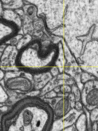
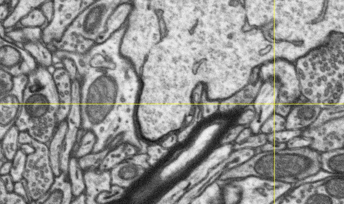
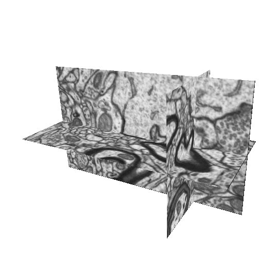
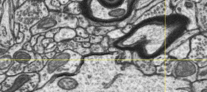
In this paper we deal with image segmentation algorithms which require laborious annotations in the form of object masks. $3$D stacks such as those depicted by Fig. 1 are common in the biomedical field and are particularly challenging, because it is difficult for users to quickly figure out what they are looking at and annotate data efficiently. In this paper, we therefore introduce a novel approach to AL that is geared towards segmenting $3$D stacks while accounting for geometric constraints of region shapes and thus making the annotation process convenient. Our approach applies both to background-foreground and multi-class segmentation of ordinary $2$D images and $3$D volumes. Our main contributions are as follows:

• We exploit geometric priors to select the image data for annotation more effectively, both for background-foreground and multi-class segmentation.

• We define novel uncertainty measures for multi-class AL, which can be combined with the above-mentioned geometric priors.

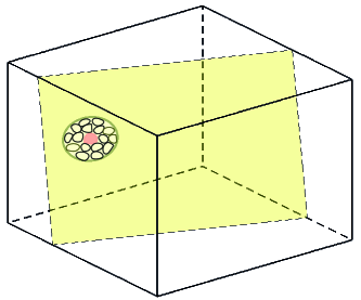
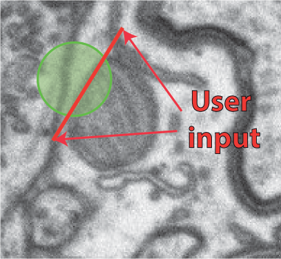
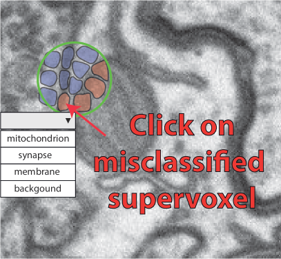
• We streamline the annotation process in $3$D volumes so that annotating them is no more cumbersome than annotating ordinary $2$D images, as depicted by Fig. 2.

The ideas on geometric uncertainty measures first appeared in [9]. Here, we extend them to the multi-class case and present in details the optimal branch-and-bound procedure for batch-mode AL. In the remainder of this paper, we first review current approaches to binary and multi-class AL and discuss why they are not necessarily the most effective when dealing with pixels and voxels. We then give a short overview of our method before discussing in details the use of geometric priors and how we search for an optimal cutting plane to simplify the annotation process. We then provide extensive experiments. We start by evaluating multi-class AL on image classification tasks and testing our geometric uncertainty with different classifiers. Then, we compare our results against those of state-of-the-art techniques in a few challenging cases in image segmentation. Finally, we provide the experiments that illustrate the role of human intuition in the labelling procedure.

Figure 2: Our approach to annotation. Top row: The system selects an optimal plane in an arbitrary orientation and presents the user with a patch that is easy to annotate. The area to annotate is shown as part of the full 3D stack. Bottom row: user interface, the planar patch the user would see. Left: in case of two classes present in the patch, it could be annotated by clicking twice to specify the red segment that forms the boundary between the inside and outside of a target object within the green circle. Right: the other way to annotate data is to correct mistakes in the current prediction. Supervoxels predicted to be mitochonria are shown in red, background in blue. If a user clicks on the misclassified supervoxel he can select the correct class among proposed. Best viewed in color as most figures in this paper.

2 Related work and motivation

Image segmentation, both background-foreground and semantic segmentation, is a fundamental problem in computer vision. Training data for learning-based segmentation algorithms usually comes in a form of pixel-wise masks which are known to be very tedious to produce. In this paper, we are concerned with situations where domain experts are available to annotate images to train image segmentation algorithms. When experts’ time is the most expensive/scarcest resource, AL is the technique of choice because it seeks the smallest possible set of training samples to annotate for effective model instantiation [10].

Active learning (AL)   Typical AL strategies for query selection rely on uncertainty sampling [11], which works remarkably well in many cases [12, 5], query-by-committee, which does not require probability estimates [13, 7], expected model change [14, 6], or measuring information in the Fisher matrix [15]. While there is a wide range of literature on AL for binary classification, multi-class problems are considered less often. Multi-class scenarios are often approached by reducing the problem to one-vs.-all binary classification [16, 17]. Alternative methods rely on the expected reduction in misclassification risk and are independent of the number of classes [4]. Unfortunately, they can run in reasonable time only when they are combined with a classifier that has an easy model update rule for adding new samples. On the other side, for uncertainty sampling, one needs to redefine the notion of uncertainty or disagreement [10, 18, 19, 20, 21, 22]. Three ways to define the most uncertain datapoint are introduced in [10]: ($1$) maximum entropy of posterior probability distribution over classes, ($2$) minimal probability of selected class and ($3$) minimal gap between the two most probable classes. There are many works relying on one of the above criteria or on combining them. This includes selection uncertainty [21], posterior distribution entropy [18, 20], the combination of entropy, minimum margin and exploration criteria [19], and all three strategies of  [10] together [22].

Recent work has demonstrated the effectiveness of data-driven AL approaches [23, 24]. These methods learn strategies from available annotated data. It learns what kind of datapoints are the most beneficial for training the model given the current state of the classification problem. Then, past experience helps to derive more effective selection strategies.

Batch-mode AL   Many interactive annotation pipelines suffer from long model update times which are necessary at every iteration. Batch-mode selection has become a standard way to increase efficiency by asking the expert to annotate more than one sample at every iteration [25, 26, 12, 27, 28, 29]. This procedure amortises the total retraining time over many annotations and enables to annotate data in parallel by several annotators. Besides, in some situations it is easier for humans to provide labels to groups of examples [30]. Density-based AL strategies often deal with the question how to form batches that ensure the diversity of the selection [27, 29, 31]. Moreover, batches can be formed with hierarchical clustering [32] and annotator’s cognitive efforts can be taken into account [33].

AL and image priors   The AL techniques have been used for tasks in computer vision such as image classification [18, 16, 4, 7], visual recognition [19, 17], semantic segmentation [34, 35], and foreground segmentation [36]. However, selection strategies are rarely designed to take advantage of image specificities when labelling individual pixels or voxels, such as the fact that a neighborhood of pixels/voxels tends to have homogeneous labels. The segmentation methods presented in [37, 35, 38] do take such geometric constraints into account for classification purposes, but not to guide AL, as we do.

Recently several authors realised the need to account for image properties in the AL selection for various computer vision tasks. For example, in human pose estimation the uncertainty depends on the spatial distribution of the detected body joints [39]. In brain connectome reconstruction, an algorithm of Plaza[40] can benefit from priors on how synapses can be situated in an image volume to result in a feasible reconstruction. Some methods [29, 36, 41] account for the influence of neighbouring instances in AL selection by connecting datapoints in a graph as we do. However, the serious difference to our approach is that they add edges between datapoints in a graph based on their feature similarity and not their geometric proximity as we do.

Human-computer interactions for segmentation   To understand how the cost of the annotation influences the final segmentation, Zlateski [42] study the performance of a convolutional neural network depending on the amount and coarseness of the training labels. In order to reach the same prediction quality, the number of annotations can be traded for their precision. However, the performance improves when more time is spent on annotations.

Instead of pixel-wise masks some works try to adapt cheaper data modalities. Scribbles (sparsely provided annotated pixels) are known to be very user-friendly to annotate images and video [43, 44, 45]. Scribbles annotations can be propagated from labelled to unlabelled pixels using a graphical model [43]. In video segmentation, scribbles are propagated though the video while preserving its consistency [45]. Another cheap annotation modality for segmentation is point-clicks [46, 47, 48]. Point-clicks on the object of interest can be incorporated into a weakly-supervised CNN with a special form of loss function [46]. If an algorithm computes many hypotheses of the segmentation, the annotator can click on the object boundaries to eliminate wrong hypotheses [49]. Polygons and pixel-wise masks are complementary label modalities: one-to-one correspondence between them can be easily established by assigning a mask to the area inside a polygon or by approximating the borders of a mask by a polygon. Then, the segmentation can be obtained either by predicting a class of pixels or by predicting the vertices of polygon with supervised [50] or reinforcement learning [51]. The polygon prediction task can involve the annotator to correct wrongly predicted vertices.

Batch-mode AL and image priors   Batch-mode AL has been mostly investigated in terms of semantic queries without due consideration to the fact that, in image segmentation, it is much easier for annotators to quickly label many samples in a localized image patch than having to annotate random image locations. We believe that for the efficient annotation pipeline in image segmentation, it is necessary to join the benefits of batch-mode AL and human-computer interactions. If samples are distributed randomly in a $3$D volume, it is extremely cumbersome to labels them using current image display tools such as the popular FIJI platform depicted by Fig. 1. Thus, in $3$D image volumes [37, 35, 52], it is important to provide the annotator with a patch in a well-defined plane, such as the one shown in Fig. 2. The technique of [53] is an exception in that it asks users to label objects of interest in a plane of maximum uncertainty. Our approach is similar, but has several distinctive features. First, the procedure we use to find the plane requires far fewer parameters to be set, as discussed in Sec. 5. Second, we search for the most uncertain patch in the plane and do not require the user to annotate the whole plane. Finally, our approach can be used in conjunction with an ergonomic interface that requires at most three mouse clicks per iteration when two classes are involved. Also, as we show in the result section, our method combined with geometric smoothness priors outperforms the earlier one.

3 Approach

We begin by broadly outlining our framework, which is set in a traditional AL context. That is, we wish to train a classifier for segmentation purposes, but have initially only few labelled and many unlabelled training samples at our disposal.

AL seeks to find, iteratively and adaptively, a small set of training samples to be annotated for effective model training [10]. In practice, this means that instead of asking an oracle to annotate all the data, we carefully select which datapoints should be labelled next based on what we know so far. The intelligent selection of data to be annotated can help to reach a good model performance using fewer labels.

In our work the AL procedure is set in the context of image segmentation. Since segmentation of $3$D volumes is computationally expensive, supervoxels have been extensively used to speed up the process [54, 55]. In the remainder of this section and in Sec. 4, we will refer almost solely to supervoxels for simplicity but the definitions apply equally to superpixels when dealing with $2$D images. We formulate our problem in terms of classifying supervoxels as a part of a specific target object. As such, we start by oversegmenting the image volume using the SLIC algorithm [56] and computing for each resulting supervoxel $s_{i}$ a feature vector $\mathbf{x}_{i}$. When dealing when with ordinary $2$D images, we simply replace the $3$D supervoxels with $2$D superpixels, which SLIC can also produce. Our AL problem thus involves iteratively finding the next set of supervoxels that should be labelled by an expert to improve segmentation performance as quickly as possible. To this end, our algorithm proceeds as follows:

1. Train a classifier on the labelled supervoxels $S_{L}$ and use it to predict the class probabilities for the remaining supervoxels $S_{U}$.

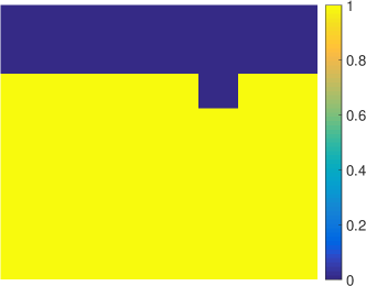
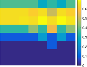
2. Score $S_{U}$ on the basis of a novel uncertainty function that we introduce in Sec. 4. It is inspired by the geometric properties of images in which semantically meaningful regions tend to have smooth boundaries. Fig. 3 illustrates its behaviour given a simple prediction map: Non-smooth regions between various classes tend to be assigned the highest uncertainty scores.

3. In volumes, select a $2$D plane that contains a patch with the most uncertain supervoxels, as shown in Fig. 2 and, in regular images, select a patch around the most uncertain superpixel. The expert can then effortlessly label an indicated $2$D patch without having to examine the image data from multiple perspectives, as would be the case otherwise and as depicted by Fig. 1. Furthermore, we can then design a simple interface that lets the user label supervoxel or superpixel batches with just a few mouse clicks, as shown in Fig. 2 and described in Sec. 6.

4. Sets $S_{L}$ and $S_{U}$ are updated and the process is repeated until the segmentation quality is satisfactory.

Compared to the standard AL procedure, our contribution lies in the way how we defined the uncertainty measure by relying on image priors (Sec. 4) and how we select a batch for annotation by designing an ergonomic interface to jointly present informative datapoints (Sec. 5).

Figure 3: Geometry-based uncertainty score. Left: predicted binary classification map for an $8\times 8$ image. In this example the classifier assigns the pixels coloured in yellow to class $1$ with probability $1$ and pixels coloured in blue to class $0$, also with probability $1$. Feature uncertainty has the lowest possible uncertainty value for all pixels as the classifier is certain of its predictions. Right: geometric uncertainty score of Section 4.3. The area of transition between the two classes is given a high geometric uncertainty score. Its maximum is reached where the boundary is not smooth.

4 Geometry-based active learning

Most AL methods were developed for general tasks and operate exclusively in feature space, thus ignoring the geometric properties of images and more specifically their geometric consistency. We start from Uncertainty Sampling (US). It is designed to focus the annotators’ attention on samples for which image features do not yet provide enough information for the classifier to decide what label to assign them. It selects samples that are uncertain in feature space to be annotated first so that classifier is updated with the largest amount of information. In short, US suggests labelling samples that are the most uncertain for the classifier, for example, closest to the classifier’s decision boundary. We will refer to this family of approaches as Feature Uncertainty (FUn). These methods are both effective and computationally inexpensive, thus, they are chosen as a basis of our work. However, they do not account for image geometry to clue which samples may be mislabelled.

To remedy this, we first introduce the concept of Geometric Uncertainty (GUn) and then show how to combine it with FUn. Our basic insight is that supervoxels that are assigned a label different from that of their neighbours ought to be considered more carefully than those that are assigned the same label, as illustrated by Fig. 3. In this $2$D toy example, standard uncertainty in the feature space is low for all pixels because the classifier is confident in its predictions. On the contrary, in terms of geometry-based uncertainty measure, pixels near classification boundaries are uncertain and those near irregular parts of the boundary are even more uncertain. This corresponds to the intuition that object boundaries should be smooth.

We express both kinds of uncertainties in terms of entropy so that we can combine them in a principled way. Doing this in multi-class segmentation case requires a new criterion for feature uncertainty, which we introduce below.

4.1 Uncertainty measures

For each supervoxel $s_{i}$ characterised by feature vector $\mathbf{x}_{i}$ and each possible label $\hat{y}\in Y$, let $p(y_{i}=\hat{y}\mid\mathbf{x}_{i})$ be the probability that the label $y_{i}$ of $s_{i}$ is $\hat{y}$. In this section we are not concerned with the question of how this probability is obtained. For background-foreground segmentation, we take $Y$ to be $\{0,1\}$. In the multi-class scenario, $Y$ is a larger set, such as $\{$background, hair, skin, eyes, nose, mouth$\}$ for face segmentation. We describe below three entropy-based uncertainty measures. We start from the well-known Shannon Entropy of the predicted distribution over all possible classes and we then introduce two novel uncertainty measures which are both entropic in nature, but account for different properties of the predicted probability distribution.

4.1.1 Total Entropy

The simplest and most common way to estimate uncertainty is to compute the Shannon entropy $\mathcal{H}$ of the total probability distribution over classes

$$\mathcal{H}(\{p(y_{i}=\hat{y}\mid\mathbf{x}_{i})\})=$$ (1)

$$-\sum_{\hat{y}\in Y}p(y_{i}=\hat{y}\mid\mathbf{x}_{i})\log p(y_{i}=\hat{y}\mid\mathbf{x}_{i}),$$

which we will refer to as Total Entropy. By definition, it is not restricted to the binary case and can be used straightforwardly in the multi-class scenario as well.

4.1.2 Selection Entropy

When there are more than two elements in $Y$, another way to evaluate uncertainty is to consider the label $b_{1}$ with highest probability: $p(y_{i}=b_{1}\mid\mathbf{x}_{i})\geq p(y_{i}=b_{j}\mid\mathbf{x}_{i})\forall b_{j}\in Y,b_{j}\neq b_{1}$, against all others taken together: $p(y_{i}=\overline{b_{1}}\mid\mathbf{x}_{i})=\sum_{b_{j}\in Y\setminus b_{1}}p(y_{i}=b_{j}\mid\mathbf{x}_{i})$. For $b_{k}\in\{b_{1},\overline{b_{1}}\}$ this yields a probability distribution

$$p_{s}=p(y_{i}=b_{k}\mid\mathbf{x}_{i}).$$ (2)

Then, we compute the entropy of the resulting probability distribution over two classes as Selection Entropy $\mathcal{H}_{s}$

$$\mathcal{H}_{s}=\mathcal{H}(p_{s}).$$ (3)

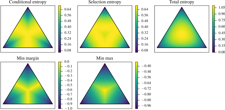
This definition of uncertainty is motivated by our desire to minimize the number of misclassified samples by concentrating on the classifier’s decision output. Notice that Selection Entropy avoids choosing the datapoints with the equal probability assigned to every class: $p(y_{i}=b_{j}\mid\mathbf{x}_{i})=p(y_{i}=b_{l}\mid\mathbf{x}_{i})\forall b_{j},b_{l}\in Y$, when the number of classes is greater than two. This makes sense in practice because an example that is confused between all classes of the multi-class problem is likely to be an outlier.

4.1.3 Conditional Entropy

Let $b_{1}$ and $b_{2}$ be two highest ranked classes for a supervoxel $s_{i}$, i.e. classes with the highest predicted probabilities: $p(y_{i}=b_{1}\mid\mathbf{x}_{i})>p(y_{i}=b_{2}\mid\mathbf{x}_{i})>p(y_{i}=b_{j}\mid\mathbf{x}_{i}),\forall b_{j}\neq b_{1},b_{2}$. Another way to evaluate uncertainty in a multi-class scenario is to consider how much more likely class $b_{1}$ is than class $b_{2}$. We assume that one of them is truly the correct class $y_{i}^{*}$, and we condition on this fact. For $\forall b_{k}\in\{b_{1},b_{2}\}$ this yields

$$p_{c}=p(y_{i}=b_{k}\mid\mathbf{x}_{i},y_{i}^{*}\in \{b_{1},b_{2}\})=$$ (4)

$$\frac{p(y_{i}=b_{k}\mid\mathbf{x}_{i})}{p(y_{i}=b_{1}\mid\mathbf{x}_{i})+p(y_{i}=b_{2}\mid\mathbf{x}_{i})}.$$

We then take the Conditional Entropy uncertainty to be the Shannon entropy of this probability distribution, which is

$$\mathcal{H}_{c}=\mathcal{H}(p_{c}).$$ (5)

This definition of uncertainty is motivated by the fact that the classifier is rarely confused about all possible classes. More typically, there are two classes that are hard to distinguish and we want to focus on those

Figure 4: Measures of Feature Uncertainty in a three-class problem. In each triangle the color denotes the uncertainty as a function of the three probabilities assigned to each class, which sum to 1. The three corners correspond to a point with probability $1$ belonging to one of the three classes and therefore no uncertainty. By contrast, the center point can belong to any class with equal probability and therefore yields maximal uncertainty. For better comparison, we inverted some values such that yellow corresponds to higher uncertainty and dark blue to the lower uncertainty. Top: entropy-based measures of Sec. 4.1, Bottom: Measures proposed in [10].

4.2 Feature Uncertainty (FUn)

In practice, we estimate $p(y_{i}=\hat{y}\mid\mathbf{x}_{i})$ by means of a classifier trained using parameters $\theta$ and we denote the distribution probability by $p_{\theta}$. Then, any of the uncertainty measures from Sec. 4.1 can be applied to the probability distribution $p_{\theta}(y_{i}=\hat{y}\mid\mathbf{x}_{i})\forall\hat{y}\in Y$ resulting in Feature Total Entropy $\mathcal{H}$ from Eq. (4.1.1), Feature Selection Entropy $\mathcal{H}_{s}$ from Eq. (3) and Feature Conditional Entropy $\mathcal{H}_{c}$ from Eq. (5). While all Feature Uncertainty measures are equivalent in the binary classification case, they behave quite differently in a multi-class scenario, as shown in the top row of Fig. 4. Furthermore, even though our Selection Entropy and Conditional Entropy measures are in the same spirit as the Min margin and Min max measures of [10] (bottom row of Fig. 4), their selection is still different and they enable the combination with geometric priors, as we will shown in Sec. 4.4. Next, we will refer to any one of these three uncertainty measures as the Feature Uncertainty $\mathcal{H}^{\theta}$.

4.3 Geometric Uncertainty

Estimating the uncertainty as described above does not explicitly account for correlations between neighbouring supervoxels. To account for them, we can estimate the entropy of a different probability, specifically the probability that supervoxel $s_{i}$ belongs to class $\hat{y}$ given the classifier predictions of its neighbours and which we denote $p_{G}(y_{i}=\hat{y})$.

Figure 5: Image represented as a graph. We treat supervoxels as nodes in the graphs and edge weights between them reflect the probability of transition of the same label to a neighbour. Supervoxel $s_{i}$ has $k$ neighbours from $A_{k}(i)=\{s_{1}^{i},s_{2}^{i},..,s_{k}^{i}\}$, $p_{T}(y_{i}=\hat{y}\mid y_{j}=\hat{y})$ is the probability of node $s_{i}$ having the same label as node $s_{j}^{i}$, $p_{\theta}(y_{i}=\hat{y}\mid\mathbf{x}_{i})$ is the probability that $y_{i}$ , class of $s_{i}$, is $\hat{y}$, given only the corresponding feature vector $\mathbf{x}_{i}$

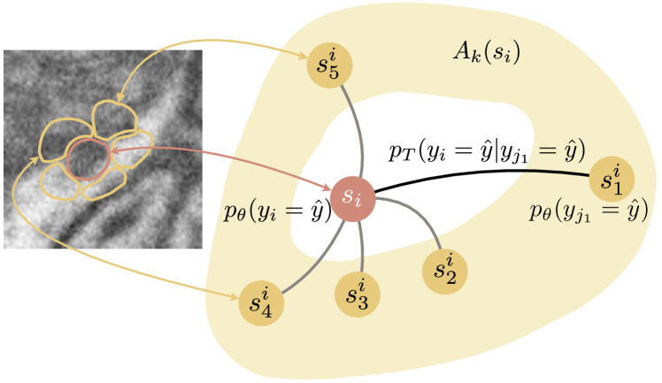
To this end, we treat the supervoxels of a single image volume as nodes of a directed weighted graph $G$ whose edges connect neighbouring supervoxels, as depicted in Fig. 5. We let $A_{k}(s_{i})=\{s^{i}_{1},s^{i}_{2},..,s^{i}_{k}\}$ be the set of $k$ nearest neighbours of $s_{i}$ and assign a weight to each edge inversely proportional to the Euclidean distance between the voxel centers. This approximation is the most precise when the supervoxels are close to being spherical, which is the case when using SLIC algorithm of [56]. For each node $s_{i}$, we normalize the weights of all incoming edges so that their sum is one. This allows to treat this quantity as the probability $p_{T}(y_{i}=\hat{y}\mid y_{j}=\hat{y})$ of node $s_{i}$ having the same label as node $s_{j}^{i}\in A_{k}(s_{i})$. It reflects our intuition that the closer two nodes are, the more likely they are to have the same label.

To define $p_{G}(y_{i}=\hat{y})$ we use a random walk procedure on graph $G$ [57], as it reflects well our smoothness assumption and has been extensively used for image segmentation purposes [58, 53]. Given the $p_{T}(y_{i}=\hat{y}\mid y_{j}=\hat{y})$ transition probabilities, we can compute the probabilities $p_{G}$ iteratively by initially taking $p^{0}_{G}(y_{i}=\hat{y})$ to be $p_{\theta}(y_{j}=\hat{y}\mid\mathbf{x}_{j})$ and then iteratively computing

$$p^{\tau+1}_{G}(y_{i}=\hat{y})=\sum_{s_{j}\in A_{k}(s_{i})}p_{T}(y_{i}=\hat{y}\mid y_{j}=\hat{y})p^{\tau}_{G}(y_{j}=\hat{y}).$$ (6)

Note that $p_{\theta}(y_{j}=\hat{y}\mid\mathbf{x}_{j})$, $p^{0}_{G}(y_{i}=\hat{y})$ and $p^{\tau+1}_{G}(y_{i}=\hat{y})$ are vectors whose dimension is the cardinality of $Y$, the set of all possible labels. The procedure described by Eq. (6) is essential for defining the geometric uncertainty as it propagates the labels of individual supervoxels into their neighborhood. Then, the supervoxels that are surrounded by neighbours whose predictions contradict to each other would receive contradicting scores and $p_{G}(y_{i}=\hat{y})$ would result in high uncertainty. The number of iterations, $\tau_{max}$, defines the radius of the neighborhood involved in the computation of $p_{G}$ for $s_{i}$, thus encoding smoothness priors. When segmenting some objects of interest, $\tau_{max}$ should be chosen approximately as the average size of these objects. This enables score propagation inside the object, but does not favour propagation from parts that are far outside of object boundaries. In our experiments, $\tau_{max}$ value varies between $10$ and $20$ depending on the application. Fig. 3 shows the result of this computation for a simple $8\text{\times}8$ image with initial prediction of a classifier as shown on the left and $k=4$ neighbours with equal edge weights. We apply $\tau_{max}=4$ iterations and the resulting geometric uncertainty on the right shows how smoothness prior is reflected in the uncertainty: non-smooth boundaries receive the highest uncertainty score.

Given these probabilities, we can use the any of the uncertainty measures of Sec. 4.1.1,  4.1.2 and 4.1.3 to compute the Geometric Uncertainty $\mathcal{H}^{G}$ for the probability distribution $p_{G}(y_{i}=\hat{y}\mid\mathbf{x}_{i})\forall\hat{y}\in Y$ as Geometric Total Entropy $\mathcal{H}$, Geometric Selection Entropy $\mathcal{H}_{s}$ and Geometric Conditional Entropy $\mathcal{H}_{c}$, respectively.

4.4 Combining Feature and Geometric Entropy

Finally, given a trained classifier, we can estimate both FUn and GUn. To use them jointly, we should in theory estimate the joint probability distribution $p_{\theta,G}(y_{i}=\hat{y}\mid x_{i})$ and the corresponding joint entropy. As this is not modelled by our classification procedure, we take advantage of the fact that the joint entropy is upper bounded by the sum of individual entropies $\mathcal{H}^{\theta}$ and $\mathcal{H}^{G}$. Thus, for each supervoxel, we take the Combined Uncertainty (CUn) to be

$$\mathcal{H}^{\theta,G}=\mathcal{H}^{\theta}+\mathcal{H}^{G},$$ (7)

that is the upper bound of the joint entropy. The same rule can be equally applied to the Total entropy and entropy-based functions Selection Entropy and Conditional Entropy. If we directly sum up feature and geometric scores defined by Min margin and Min max of Settles [10], the resulting measure does not have a physical meaning. The combined uncertainty measure is more appealing thanks to its upper bound interpretation.

In practice, using this measure means that supervoxels that individually receive uncertain predictions and are in areas of non-smooth transition between classes will be considered first. Note that the AL method of [31] based on Zhou’s propagation [38], which is similar to the one we use, operates exclusively on $\mathcal{H}^{G}$. However, we experimentally observed on our datasets that considering the upper bound on the joint entropy from Eq. 7 results in a significant improvement in the learning curve compared to single Feature or Geometric uncertainty alone. Our MATLAB implementation of Combined Total Entropy on $10$ volumes of resolution $176\text{\times}170\text{\times}220$ of the MRI dataset from Sec. 6.5.2 takes $1.4$s per iteration ($2.3$ GHz Intel Core i$7$, $64$-bit). The possibility of real-time performance is extremely important in the interactive applications.

5 Batch-mode geometry query selection

(a)	(b)	(c)

Figure 6: a) Parametrizing the search space. A circular patch is defined as the intersection of a plane with a sphere. Plane $p_{i}$ (yellow) is parametrised by two angles, $\phi$ and $\gamma$; $\phi$ is the angle between the negative component of axis $-Y$ and plane intersection with $XY$ (blue), similarly, $\gamma$ is the angle between $-Z$ and plane intersection with $YZ$ (red). b) Corridor. A corridor is a union of the areas between planes $p_{1}$ and $p_{4}$ as well as between $p_{2}$ and $p_{3}$. The green points depict supervoxels included in corridor $\Omega$ while black points depict supervoxels outside of it. c) Bounding function and corridor splitting procedure. The score of the plane $p_{0}$ is less or equal to the score of all the points included between two planes $p_{\min}$ and $p_{\max}$: $U(p_{0})<U(\Omega)$. We split the corridor $\Omega$ into corridors $[\phi_{\min},\phi_{0})\times[\gamma_{min},\gamma_{0})$, $[\phi_{\min},\phi_{0})\times[\gamma_{0},\gamma_{\max})$, $[\phi_{0},\phi_{\max})\times[\gamma_{min},\gamma_{0})$ and $[\phi_{0},\phi_{\max})\times[\gamma_{0},\gamma_{\max})$ and evaluate their uncertainty values. Among all available sectors we select a sector with the highest value to be split next. Best seen in color.

The straightforward way to exploit the CUn from Sec. 4.4 would be to pick the most uncertain supervoxel, ask the expert to label it, retrain the classifier, and iterate. A more effective way is to find appropriately-sized batches of uncertain supervoxels and ask the expert to label them all at once before retraining the classifier. As discussed in Sec. 2, this is referred to as batch-mode selection, which usually reduces the time-complexity of AL. However, a naive implementation would force the user to randomly view and annotate several supervoxels in $3$D volumes regardless of where they are. This would not be user friendly as they would have to navigate a large image volume at each iteration.

In this section, we therefore introduce an approach to select an uncertain planar patch in $3$D volumes and allow the user to quickly label supervoxels within it, as shown in Fig. 2. We allow annotator to only consider circular regions within planar patches such as the one depicted in Figs. 2 and 13. These can be understood as the intersection of a sphere with a plane of arbitrary orientation.

Recall from Sec. 4, that we can assign to each supervoxel $s_{i}$ an uncertainty estimate $U(s_{i})$ in one of several ways. Whichever one we choose, finding the circular patch of maximal uncertainty $p^{\ast}$ can be formulated as finding

$$p^{\ast}=\operatorname*{arg\,max}_{p}\sum_{s_{j}\in p}U(s_{j}),$$ (8)

where the summation occurs over the voxels that intersect the plane and are within the sphere.

Since Eq. (8) is linear in $U(s_{j})\geq 0$, we design a branch-and-bound procedure to finding the plane that yields the largest uncertainty. It recursively eliminates whole subsets of planes and quickly converges to the correct solution. Whereas an exhaustive search would be excruciatingly slow, our current MATLAB implementation on MRI dataset takes $0.024$s per plane search with the same settings as in Sec. 4.4. This means that a C implementation of the entire pipeline would be real-time, which is critical for acceptance of such an interactive method by users.

As discussed above, this procedure could be used in conjunction with any one of the uncertainty measures defined in the previous section. We will as shown in Sec. 6 that it is most beneficial when used in combination with the geometry-aware criterion of Sec. 4.4. We describe our branch-and-bound plane-finding procedure in more detail below and in Section 5.3 we show a simplified example of this procedure in $2$D.

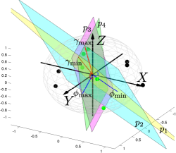
5.1 Parametrizing the search space

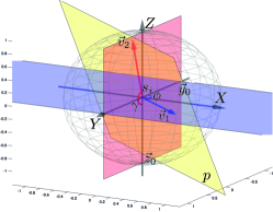
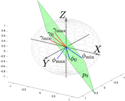
Let us consider a spherical volume centered at supervoxel $s_{i}$, such as the one depicted by Fig. 6a. Since the SLIC superpixels/supervoxels are always roughly circular/spherical, any supervoxel $s_{j}$ can be well approximated by a sphere of radius $\kappa$, set to a constant for a particular dataset, and its center $w_{j}$. We will refer to this approximation as $\hat{s}_{j}$. Then, every $\hat{s}_{j}=(w_{j},\kappa)$ is characterized by its center $w_{j}$ and the common radius $\kappa$.

Let $\hat{S}_{i}^{r}$ be the set of supervoxels within the distance $r$ from $\hat{s}_{i}$, that is,

$$\hat{S}_{i}^{r}=\{\hat{s}_{j}=(w_{j},\kappa)\mid\|w_{j}-w_{i}\|\leq r\}.$$ (9)

If we take the desired patch size to be $r$, we can then operate exclusively on the elements of $\hat{S}_{i}^{r}$. Let $P_{i}$ be the set of all planes passing through the center of $\hat{s}_{i}$. As we will see below, our procedure requires defining planes, area splits of approximately equal size, and supervoxel membership to certain areas and planes. We parametrize planes in $P_{i}$ as follows.

Let us consider a plane $p\in P_{i}$, such as the one shown in yellow in Fig. 6a. It intersects the $XY$ plane along a line characterized by a vector $\vec{v}_{1}$, shown in blue. Without loss of generality, we can choose the orientation of $\vec{v}_{1}$ such that its $X$ coordinate is positive and we denote by $\phi$ the angle between the negative component of axis $-Y$ and $\vec{v}_{1}$. Similarly, let us consider the intersection of $p$ with $YZ$ plane and characterize it by the vector $\vec{v}_{2}$ (shown in red) with a positive $Y$ coordinate. Now let $\gamma$ be the angle between $-Z$ and $\vec{v}_{2}$. We can now parametrize the plane $p$ by the two angles $\phi\in[0,\pi)$ and $\gamma\in[0,\pi)$ because there is one and only one plane passing through two intersecting lines. We will refer to $(\phi,\gamma)$ as the plane’s angular coordinates. Finally, let $C_{i}^{r}(p)$ be the set of supervoxels $\hat{s}_{j}\in\hat{S}_{i}^{r}$ lying on $p$, that is,

$$C_{i}^{r}(p)=\{\hat{s}_{j}\in\hat{S_{i}^{r}}\mid\text{distance(}p,w_{j}\text{)}\leq 2\kappa\}.$$ (10)

The set $P_{i}$ can be represented by the Cartesian product $[0,\pi)\times[0,\pi)$ of the full ranges of $\phi$ and $\gamma$. Let $\Phi=[\phi_{\min},\phi_{\max})$ and $\Gamma=[\gamma_{\min},\gamma_{\max})$ be two angular intervals. We will refer to a set of planes with angular coordinates in $\Phi\times\Gamma$ as the corridor $\Omega=\Phi\times\Gamma$, as illustrated by Fig. 6b. The boundaries of this corridor are defined by four planes shown in Fig. 6b: $p_{1}=(\phi_{\min},\gamma_{\min})$, $p_{2}=(\phi_{min},\gamma_{\max})$, $p_{3}=(\phi_{\max},\gamma_{min})$ and $p_{4}=(\phi_{\max},\gamma_{\max})$.

5.2 Searching for the best bisecting plane

5.2.1 Uncertainty of planes and corridors

Recall that we assign to each supervoxel $\hat{s}_{j}$ an uncertainty value $U(\hat{s}_{j})\geq 0$. We take the uncertainty of plane $p$ to be

$$U(p)=\sum\limits_{\hat{s}_{j}\in C_{i}^{r}(p)}U(\hat{s}_{j}).$$ (11)

Finding a circular patch $p^{*}$ of maximum uncertainty then amounts to finding

$$p^{*}=(\phi^{*},\gamma^{*})=\underset{p\in P_{i}}{\arg\max}\ U(p).$$ (12)

Similarly, we define the uncertainty of a corridor as the sum of the uncertainty values of all supervoxels lying between the four planes bounding it, between $p_{1}$ and $p_{4}$, and between $p_{2}$ and $p_{3}$ as depicted by green points in Fig. 6b. We therefore write

$$U(\Omega)=\sum\limits_{\hat{s}_{j}\in C_{i}^{r}(\Omega)}U(\hat{s}_{j}),$$ (13)

where $C_{i}^{r}(\Omega)$ represents the supervoxels lying between the four bounding planes. In practice, a supervoxel is considered to belong to the corridor if its center lies either between $p_{1}$ and $p_{4}$ or between $p_{2}$ and $p_{3}$, or is no further than $\kappa$ away from any of them. When the angles are acute, the membership of a voxel is decided by checking that the dot product of the voxel coordinates with the plane normals have the same sign, provided that the normals orientations are chosen so that they all point inside the corridor.

5.2.2 Branch-and-bound

To solve Eq. 12 and find the optimal circular patch, we use a branch-and-bound approach. It involves quickly eliminating entire subsets of the parameter space $\Phi\times\Gamma$ using a bounding function [59], a recursive search procedure, and a termination criterion, which we describe below.

Bounding function   Let us again consider the corridor $\Omega=[\phi_{\min},\phi_{\max})\times[\gamma_{\min},\gamma_{\max})$ bounded by the four planes $p_{1}$ to $p_{4}$. Let us also introduce the plane $p_{0}=(\alpha_{1}\phi_{\min}+\beta_{1}\phi_{\max},\alpha_{2}\gamma_{\min}+\beta_{2}\gamma_{\max})$, where $\alpha_{1}+\beta_{1}=1,\alpha_{2}+\beta_{2}=1$ depicted by Fig. 6c. Given that $U(\hat{s}_{j})\geq 0$ and that Eq. 12 is linear in $U(\hat{s}_{j})$, the uncertainty of $p_{0}$ will always be less or equal to that of $\Omega$. This allows us to bound the uncertainty of any plane from above and to search for the solution only within the most promising parameter intervals.

Search procedure   As in work of [59], we maintain a priority queue $L$ of corridors. At each iteration, we pop the corridor $\Omega_{\max}^{j}=[p_{1}^{j},p_{2}^{j},p_{3}^{j},p_{4}^{j}]$ with the highest uncertainty $U(\Omega_{\max}^{j})$ according to Eq. 13 and process it as follows.

We introduce two new angles $\phi_{0}^{j}=(\phi_{\min}^{j}+\phi_{\max}^{j})/2$ and $\gamma_{0}^{j}=(\gamma_{\min}^{j}+\gamma_{\max}^{j})/2$ and split the original parameter intervals into two, as shown in Fig. 6c. We compute the uncertainty of four corridors: $[\phi_{\min},\phi_{0})\times[\gamma_{min},\gamma_{0})$, $[\phi_{\min},\phi_{0})\times[\gamma_{0},\gamma_{\max})$, $[\phi_{0},\phi_{\max})\times[\gamma_{min},\gamma_{0})$ and $[\phi_{0},\phi_{\max})\times[\gamma_{0},\gamma_{\max})$, and add them to the priority queue $L$.

Note, that we always operate on acute angles after the first iteration with initialization $[0;\pi)$, which allows us to compute the uncertainty scores of corridors as discussed in Section 5.2.1.

Termination condition   The search procedure terminates when the bisector plane $p_{0}=(\phi_{0},\gamma_{0})$ of the corridor $C_{i}^{r}(\Omega_{\max}^{j})$ touches all the supervoxels from the corridor. To fulfil this condition it is enough to ensure that the distance from any point in the corridor to a bisector plane is within the offset $2\kappa$, that is,

$$\text{distance(}p_{0},\hat{s}_{l}\text{)}\leq 2\kappa,\forall\hat{s}_{l}\in\Omega_{\max}^{j}.$$ (14)

Since $U(p_{0})$ is greater than the uncertainty of all the remaining corridors, which is itself greater than that of all planes they contain (including the boundary cases), $p_{0}$ is guaranteed to be the optimal plane we are looking for.

5.2.3 Global optimization

Our branch-and-bound search is relatively fast for a single voxel but not fast enough to perform it for all supervoxels in a stack. Instead, we restrict our search to $t$ most uncertain supervoxels in the volume.

We assume that the uncertainty scores are often consistent in small neighbourhoods, which is especially true for the geometry-based uncertainty of Section 4.3. By doing so it enables us to find a solution that is close to the optimal one with a low value of $t$. In this way, the final algorithm first takes all supervoxels $S$ with uncertainty $U$ and selects the top $t$ locations. Then, we find the best plane for each of the top $t$ supervoxels and choose the best plane among them.

5.3 Illustration of search procedure in $2$D

(a)	(b)	(c)
(d)	(e)	(f)

Figure 7: Illustration of our branch-and-bound algorithm in $2$D. a) The $2$D-equivalent of searching for a plane in sphere is searching for a line in circle. b) The bounding function states that value of a sector is not smaller than the value of a line inside it. c) The procedure starts with splitting the whole parameter interval into $2$ sectors. We compute the value of each sector and keep a priority queue of them. d) At each step of the procedure we divide the sector with the highest uncertainty in two new sectors by a bisector plane. e) and f) The procedure continues by splitting the sector with the highest value.

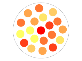
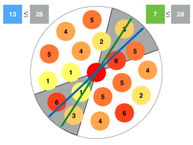
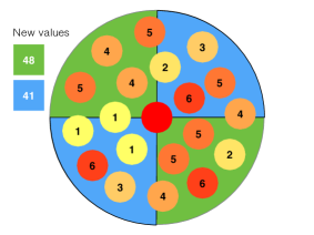
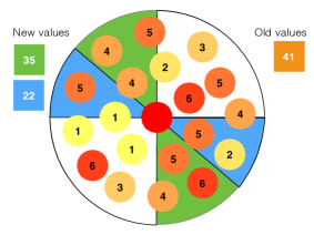
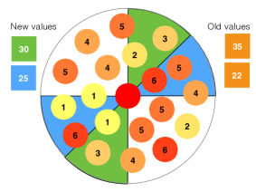
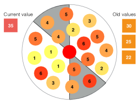
As it is difficult to represent graphically our branch-and-bound search procedure in $3$D, for illustration purposes we demonstrate it here on a $2$D example. The $2$D-equivalent of searching for a plane in sphere is searching for a line in circle.

In Figure 7(a) we show a circle with superpixels approximated by circles and where the color of each superpixel indicates how uncertain it is, with red being the most uncertain and yellow the least uncertain. Then, the task is to find a line of a maximum uncertainty, where the uncertainty of a line is defined as the sum of the uncertainties of the superpixels that it intersects. For example, Figure 7(b) demonstrates that the score of blue line is $6+1+6=13$ and the score of the green line is $3+1+3=7$. A corridor in $3$D corresponds to a sector in $2$D. An example of sector is shown in Figure 7(b) in grey with its score being $6+3+1+6+2+5+3=26$. Figure 7(b) also illustrates the bounding function condition: the score of any line inside the sector is no bigger than the score of the sector that includes this line, in our case, $13\leq 26$ and $7\leq 26$. The search procedure starts in Figure 7(c): We split the circle into blue and green sectors and compute their scores ($48$ and $41$). All the scores encountered during the search procedure are stored in a priority queue. At every iteration, the sector with the highest score is selected from the queue and split into two. For example, the green sector of Figure 7(c), whose score of $48$ is the highest, is split into two new equal sectors resulting in $3$ sectors depicted in Figure 7(d). The new uncertainty scores $35$ and $22$ are added to the priority queue. Next, the sector with the highest score is the blue sector of Figure 7(c). We split it into two new sectors in Figure 7(e). Next, we split the green sector of Figure 7(d) with the uncertainty score of $35$. The procedure continues until the sector with the highest uncertainty can fit at most one superpixel at the perimeter of the original circle as shown in Figure 8.

Figure 8: Termination condition of our branch-and-bound procedure in $2$D. The search terminates when a sector can fit at most one superpixel at the perimeter of the original circle. In this case, such a sector can be found as the one that exceeds the minimal angle $\alpha_{\min}$.

6 Experiments

In this section, we evaluate our approach on two different Electron Microscopy (EM) datasets and on one of Magnetic Resonance Imaging (MRI) dataset. We then demonstrate that CUn is also effective for natural $2$D images. In multi-class MRI and multi-class natural $2$D images of faces the extended version of our approach also results in enhanced performance.

6.1 General setup

For most of our experiments, we used Boosted Trees selected by gradient boosting [60, 61] as our underlying classifier. Nothing in our method is specific to a classifier and thus in some of the experiments we also deal with Logistic Regression and Random Forest classifiers. These general-purpose classifiers were chosen because they can be trained fast, they provide reasonable probabilistic predictions even with very small amount of training data and many features. However, there exist no closed form solution when new points are added. Thus, AL strategies such as expected model change or expected error reduction are not suitable to be applied with our classifier because they takes hours for one model update for a typical dataset size in our applications. In Gradient Boosting, given that during early AL iterations rounds, only limited amounts of training data are available, we limit the depth of our trees to $2$ to avoid over-fitting. Following standard practices, individual trees are optimized using $40$%-$60$% of the available training data chosen at random and $10$ to $40$ features are explored per split.

6.1.1 Baselines

For each dataset, we compare our approach against several baselines. The simplest is Random Sampling (Rand), which involves randomly selecting samples to be labelled. It can be understood as an indicator of how difficult the learning task is.

In practice, the most widely used AL approach is Uncertainty Sampling [11, 12, 27, 20, 19, 5]. To test several variations of it, we use several standard definitions of uncertainty described in [10]. The first involves choosing the sample with the smallest posterior probability for its predicted class $b_{1}$, that is,

$$\operatorname*{arg\,min}_{s_{i}\in S_{U}}p_{\theta}(y_{i}=b_{1}|\mathbf{x}_{i}).$$ (15)

Because of the structure of this strategy, we will refer to it as Min max: FMnMx. Uncertainty can also be defined by considering the probability difference between the first and second most highly ranked classes $b_{1}$ and $b_{2}$. The most uncertain sample is then taken to be

$$\operatorname*{arg\,min}_{s_{i}\in S_{U}}\{p_{\theta}(y_{i}=b_{1}|\mathbf{x}_{i})-p_{\theta}(y_{i}=b_{2}|\mathbf{x}_{i})\}.$$ (16)

We will refer to this Min margin strategy as FMnMar. Finally, the AL procedure can take into account the entire distribution of scores over all classes, compute the Total entropy $H$ of Sec. 4.1.1, and select

$$s^{*}=\underset{s_{i}\in S_{U}}{\arg\max}(H(s_{i})),$$ (17)

which we will refer to as FEnt. Recall that FMnMx and FMnMar cannot be easily combined with the geometric uncertainty because no upper-bound rule is applicable.

In the case of binary classification, FMnMx, FMnMar and FEnt are strictly equivalent because the corresponding expressions are monotonic functions of each other. In the multi-class scenario, however, using one or the other can result in different behaviours, as shown in [18, 19, 20, 21, 22]. According to [10], FEnt is best for minimizing the expected logarithmic loss while FMnMx and FMnMar are better suited for minimizing the expected $0$/$1$-loss.

6.1.2 Proposed strategies

All entropy-based measures introduced in Secs. 4.2 and 4.3 can be used in our unified framework. Let $H^{F}$ be the specific uncertainty measure that we use in a given experiment. The strategy then is to select

$$s^{*}=\underset{s_{i}\in S_{U}}{\arg\max}(H^{F}(s_{i})).$$ (18)

Recall that we refer to the feature uncertainty FUn strategy of Sec. 4.1 that relies on standard Total entropy as FEnt. By analogy, we will refer to those that rely on the Selection Entropy and Conditional Entropy of Eqs. 3 and 5 as FEntS and FEntC, respectively. Similarly, when using the combined uncertainty CUn of Sec. 4.4, we will distinguish between CEnt, CEntS, and CEntC depending on whether we use Total Entropy, Selection Entropy, or Conditional Entropy.

Any strategy can be applied in a randomly chosen plane, which we will denote by adding p to its name, as in pFEnt. Finally, we will refer to the plane selection strategy of Sec. 5 in conjunction with either FUn or CUn as p*FEnt, p*FEntS, p*FEntC, p*CEnt, p*CEntS and p*CEntC, depending on whether uncertainty from FEnt, FEntS, FEntC, CEnt, CEntS, or CEntC is used in the plane optimization. We will show that it does not require more than three corrections per iteration. For performance evaluation purposes, we will therefore estimate that each user intervention for p*FEnt, p*CEnt, p*FEntS, p*CEntS, p*FEntC, p*CEntC requires either two or three inputs from the user whereas for other strategies it requires only one.

Note that p*FEnt is similar in spirit to the approach [53] and can therefore be taken as a good indicator of how it would perform on our data. However, unlike in [53], we do not require the user to label the whole plane and retain our proposed interface for a fair comparison.

Before diving into the complex experimental setup with real problems that motivate our work, we first conduct a set of experiments where we study a) if the multi-class uncertainty criteria are efficient in general multi-class classification, and b) if the geometry-based uncertainty is applicable with various classifiers.

6.2 Multi-class active learning

Figure 9: Sample images from the image-classification datasets Chinese, Butterflies and Digits.

Figure 10: Multi-class AL strategies applied to image classification tasks. Logistic regression is used as an underlying classifier, compare standard multi-class AL criteria to the newly introduced entropy-based criteria.

Recall from Sec. 4.1 that in multi-class scenarios, our different approaches to measuring FUn yield different results, as shown in Fig. 4. Therefore, even though all our strategies derive from the similar intuition, they favour different points. For example, FMnMar selects samples with small margin between the most probable classes irrespectively of the absolute values of the probabilities, whereas FEntC allows for bigger margins for higher values. Selection Entropy FEntS tends to avoid samples that look like they can belong to any of the existing classes. This property can be useful to avoid querying outliers that look unlikely to belong to any class.

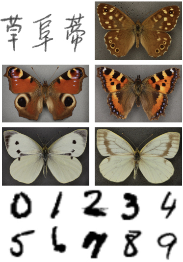
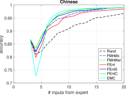
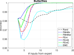
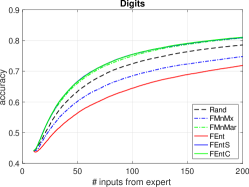
To study these differences independently of a full image segmentation pipeline, we first test the various strategies in a simple multi-class image classification task. We use them on the three datasets depicted by Fig. 9. Digits is a standard MNIST collection with $10$ hand-written digits and we use raw pixel values as features. Chinese comprises $3$ classes from the a dataset of of Chinese handwriting characters [62]. Butterflies dataset contains $5$ classes from British butterfly images from a museum collection [63]. In the Chinese and Butterflies datasets, features are extracted using a Deep Net [63, 64].

We use a logistic regression classifier and test our various AL multi-class strategies including Expected Model Change (EMC) [10, 34, 6]. The results are shown in Fig. 10. The strategies based on the Selection and Conditional Entropy perform either better or at least as well as the strategies based on the standard measures of uncertainty. The performance of EMC approach is not consistent and does not justify a high computational cost: $45$ and $310$ seconds per iteration in Chinese and Butterfly datasets with $4096$ samples with $359$ and $750$ features correspondingly, against $0.005$ and $0.01$ seconds by Conditional Entropy. The EMC execution time grows with the AL pool size and thus, we did not run experiments with more than $10\,000$ samples. Many strategies exhibit a noticeable performance drop after a few iterations of AL. The reason for this is the imbalance of the class proportions in the training set. AL starts with a small balanced datasets. Then, it is highly likely that the first annotation iterations will make the training set unbalanced. With little data, the negative influence of the class imbalance on the classifier is bigger than the advantage of adding more data. This effect is quickly eliminated when more data is collected, thus we do not concentrate on it much in the further experiments.

6.3 Geometry-based uncertainty with different classifiers

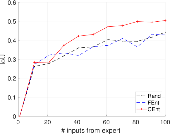
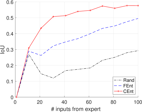
The way how scores of the classifier are propagated in the Eq. (6) implies nothing about the classifier except for producing a probabilistic prediction. However, the applications with image data are characterised by a big number of features in classification and we found various tree-based models to be well suited for these tasks when only little training data is available. To check that our Geometric uncertainty can generalise well for various type of classifiers we conduced the experiment where we compare basic versions of FEnt and CEnt with two types of classifiers. For this experiment we use striatum datasets which will be presented in details further. We use two types of classification models, Gradient Boosted Decision Trees and Random Forest. The results are presented in Fig. 11. We notice some variability in the results: while with Gradient Boosting the basic uncertainty sampling outperforms the passive data selection, with Random Forests they perform very similarly. Despite these differences, the proposed algorithm CEnt outperforms FEnt in both cases. In our next experiments we concentrate on using Gradient Boosting classifier as it demonstrated higher absolute scores in this initial study and it is reported to be successful in our applications [61].

(a) Random Forest

(b) Gradient Boosting

Figure 11: Comparison of performance of FEnt and CEnt with various classifiers. Despite the differences in scores between classifiers, geometric uncertainty consistently wins in performance.

6.4 Parameters of the strategies

6.4.1 Adaptive thresholding for binary AL

(a)

(b)

Figure 12: Threshold selection. (a) We estimate mean and standard deviation for classifier scores of positive class datapoints ($\mu^{+}$ and $\sigma^{+}$, data is shown in red) and negative class datapoints ($\mu^{-}$, $\sigma^{-}$, data is shown in blue) and fit 2 Gaussian distributions. Given their pdf, we estimate the optimal Bayesian error with threshold $h^{*}$. (b) Adaptive Thresholding convergence rate of classifier threshold for different AL strategies.

The probability of a supervoxel belonging to a certain class from Sec. 4.2 is computed as

$$p_{\theta}(y_{i}=\hat{y}|x_{i})=\frac{\exp^{-2\cdot(F_{\hat{y}}-h_{\hat{y}})}}{\sum_{y_{j}\in Y}\exp^{-2\cdot(F_{y_{j}}-h_{y_{j}})})},$$ (19)

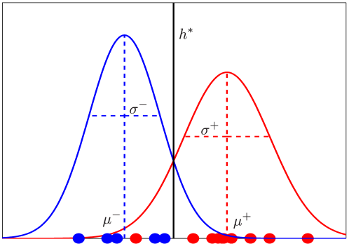
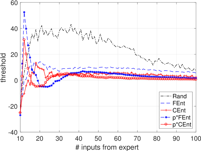
where $F=\{F_{\hat{y}}|\hat{y}\in Y\}$ is the classifier output and $h=\{h_{\hat{y}}|\hat{y}\in Y\}$ is the threshold [65]. Given enough training data, it can be chosen by cross-validation but this may be misleading or even impossible at early stages of AL. In practice, we observe that the optimal threshold value varies significantly for binary classification tasks and that the uncertainty measures are sensitive to it. By contrast, in multi-class scenarios, the threshold values remain close to $0$ and the uncertainty-based strategies are comparatively unaffected. In our experiments, we therefore take the threshold to be $0$ for multi-class segmentation and compute it as follows in the binary case. We assume that the scores of training samples in each class are Gaussian distributed with unknown parameters $\mu$ and $\sigma$. We then find an optimal threshold $h^{*}$ by fitting Gaussian distributions to the scores of positive and negative classes and choosing the value that yields the smallest Bayesian error, as depicted by Fig. 12a. We refer to this approach as Adaptive Thresholding and we use it in all our experiments. Fig. 12b depicts the value of the selected threshold as the amount of annotated data increases. Note that our various strategies yield different convergence rates, with the fastest for the plane-based strategies, p*FEnt and p*CEnt.

6.4.2 Geometric uncertainty

The average radius of supervoxels $\kappa$ is $4.3$ in EM dataset and $5.7$ in MRI dataset. Parameter $\kappa$ is computed after setting the total number of supervoxels in a volume that is chosen according to the computational budget. In general, higher number of supervoxels can allow for better segmentation accuracy but it is computationally expensive as each of the supervoxels is treated as an additional datapoint for classification. Besides, it is difficult for a human expert to annotate very small image patches reliably. We set the number $k$ of nearest neighbours of Sec. 4.3 to be the average number of immediately adjacent supervoxels on average, which is between $7$ and $15$ depending on the resolution of the image and size of supervoxels. However, experiments showed that the algorithm is not very sensitive to the choice of this parameter. For random walk inference, $\tau_{max}=10$ iterations yield the best learning rates in the multi-class case and $\tau_{max}=20$ in the binary-segmentation one.

6.4.3 Plane selection

We restrict the size of each planar patch to be small enough to contain typically not more than $2$ classes of objects and we explain what happens if this condition is not satisfied. To this end, we take the radius $r$ of Sec. 5.1 to be between $10$ and $15$. Figs. 2, 13 jointly depict what a potential user would see for plane selection strategies given a small enough patch radius. Given a well designed interface, it will typically require no more than one or two mouse clicks to provide the required feedback, as depicted by Fig. 2. The easiest way to annotate patches with only two classes is to indicate a line between them, and in situations when more than two classes co-occur in one patch, we allow users to correct mistakes in the current prediction instead. All plane selection strategies use the $t=5$ best supervoxels in the optimization procedure as described in Sec. 5. Further increasing this value does not yield any significant learning rate improvement. The parameters of branch-and-bound plane selection procedure are the radius of the patch $r$ and the number $t$ of patch centers to consider. The parameter $r$ is chosen such that it results in a convenient interface for labelling, while parameter $t$ is chosen depending on a given computational budget. Using branch-and-bound algorithm instead of gradient decent as suggested in [53] avoids setting the the learning rate and other optimization-related parameters.

Figure 13: Circular patches to be annotated by the expert highlighted by the yellow circle in Electron Microscopy and natural images. The patches can be annotated either with a line that separates 2 classes or by correcting the mistakes in the current prediction, as shown in Fig. 2.

6.4.4 Experimental protocol

We start with $5$ labelled supervoxels from each class and perform AL iterations until we receive $100$ simulated user inputs in the binary case and $200$ in the multi-class case. Each method starts with the same random subset of samples and each experiment is repeated $N=40-50$ times. We will therefore plot not only accuracy results but also indicate the variance of these results. We use half of the available data for independent testing and the AL strategy selects new training datapoints from the other half.

We have access to fully annotated ground-truth volumes and we use them to simulate the expert’s intervention in our experiments. This ground truth allows us to model several hypothetical strategies of human expert as will be shown in Sec 6.7. We detail the specific features we used for EM, MRI, and natural images in the corresponding sections.

6.5 Results on volumetric data

6.5.1 Results on EM data

Figure 14: Hippocampus volume for mitochondria segmentation.

Figure 15: Comparison of various AL strategies for (binary) mitochondria segmentation. Left: striatum dataset, right: hippocampus dataset.

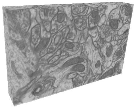
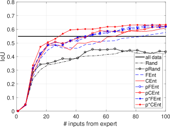
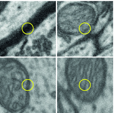
First, we consider $3$D EM stacks of rat neural tissue from the striatum and from the hippocampus. One stack of size $318\text{\times}711\text{\times}422$ ($165\text{\times}1024\text{\times}653$ for the hippocampus) is used for training and another stack of size $318\text{\times}711\text{\times}450$ ($165\text{\times}1024\text{\times}883$) is used to evaluate the performance. Their resolution is $5$nm in all three spatial orientations. The slices of Fig. 1 come from the striatum dataset and the hippocampus volume is shown in Fig. 14. Since the image have the same resolution in all dimensions, they can be viewed equally well in all orientations and specialized tools have been developed for use by neuroscientists [66].

The task is to segment mitochondria, which are the intracellular structures that supply the cell with its energy and are of great interest to neuroscientists. It is extremely laborious to annotate sufficient amounts of training data for learning segmentation algorithms to work satisfactorily. Furthermore, different brain areas have different visual characteristics, which means that the annotation process must be repeated often. The features for classification rely on local texture and shape information using ray descriptors and intensity histograms [55].

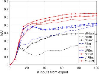
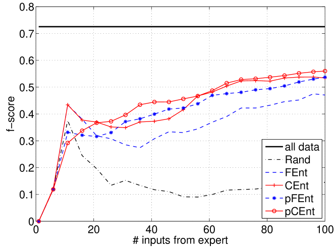
In Fig. 15, we plot the performance of all the approaches as a function of the annotation effort, where the performance is measured in terms of the intersection over union (IoU) score [67], a commonly used measure for segmentation applications. The horizontal lines at the top depict the IoU scores obtained by using the whole training set, which comprises $276\,130$ and $325\,880$ supervoxels for the striatum and the hippocampus, respectively. FEnt provides a boost over Rand and CEnt yields a larger one. Any strategy can be combined with a batch-mode AL that means that a $2$D plane is selected to be annotated. For example, strategies pRand, pFEnt and pCEnt present to the user a randomly selected $2$D plane around the sample selected by Rand, FEnt and CEnt. Addition of a plane boosts the performance of all corresponding strategies, but further improvement is obtained by selecting an optimal plane by branch-and-bound algorithm in strategies p*FEnt and p*CEnt. The final strategy p*CEnt outperforms all the rest of the strategies thanks to the synergy of geometry-inspired uncertainty criteria and the intelligent selection of a batch. Also note that the $100$ samples we use are two orders of magnitude smaller than the total number of available samples. Nevertheless AL provides a segmentation of comparable quality.

Somewhat surprisingly, in the hippocampus case, the classifier performance given only 100 training data points is higher that the one obtained by using all the training data. In fact, this phenomenon has been reported in the AL literature [68] and suggests that in some cases a well chosen subset of datapoints can produce better generalisation performance than the complete set.

Recall that the performance scores are averaged over many runs. In Table I, we give the corresponding variances. Note that both using the geometric uncertainty and the selection of optimal plane tend to reduce variance, thus making the process more predictable.

TABLE I: Variability of results (in the metric corresponding to the task) by different binary AL strategies. 80% of the scores are lying within the indicated interval. FUn is more variable that CUn, batch selection is less variable that single-instance selection and the batch-selection with an optimal plane cut combined with geometry-inspired uncertainty is the least variable. The best result is highlighted in bold.

Dataset	FEnt	CEnt	pFEnt	pCEnt	p*FEnt	p*CEnt
Striatum	$0.133$	$0.105$	$0.121$	$0.094$	$0.115$	0.086
Hippoc.	$0.117$	$0.101$	$0.081$	$0.092$	$0.090$	0.078
MRI	$0.076$	$0.064$	$0.078$	$0.074$	$0.073$	0.048
Natural	$0.145$	$0.140$	$0.149$	0.124	—	—

6.5.2 Results on MRI data

Figure 16: MRI data for tumor segmentation (Flair image).

In this section, we consider multi-modal brain-tumor segmentation in MRI brain scans an example of which is depicted in Fig. 16. Segmentation quality critically depends on the amount of training data and only highly-trained experts can provide it. We use the BRATS dataset where T$1$, T$2$, FLAIR, and post-Gadolinium T$1$ MR images are available for each of $20$ subjects [69]. We use standard filters such as Gaussian, gradient filter, tensor, Laplacian of Gaussian and Hessian with different parameters to compute the feature vectors we feed to the Boosted Trees. Notice that we use different features compared to EM images that demonstrates that our method can be applied in different applications.

Foreground-background segmentation  

Figure 17: Comparison of various AL strategies for MRI data for binary tumor segmentation. Right: dice score for BRATS2012 dataset, left: ${\bf p*CEnt}$ strategy with patches of different radius.

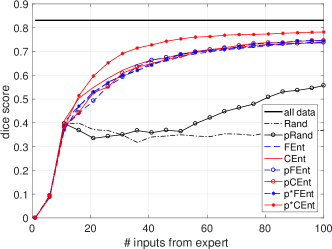
We first consider segmentation of tumor versus healthy tissue. In Fig. 17, left we plot the performance of all the approaches as a function of the annotation effort where performance is measured in terms of the dice score [52], a commonly used quality measure for brain tumor segmentation. In Table I we give the corresponding variances. We observe the same pattern as in Fig. 15, with p*CEnt again resulting in the highest score. Note that difference between p*CEnt and pCEnt is greater than between p*FEnt and pFEnt in all the experiments. This is the evidence of the synergy brought by the geometric uncertainty and the batch selection based on the geometry.

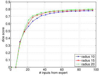
The patch radius parameter $r$ of Sec. 5.1 plays an important role in plane selection procedure. To evaluate its influence, we recomputed our p*CEnt results $50$ times using three different values for $r=10$, $15$ and $20$. The resulting plot is shown in Fig. 17 on the right. As expected, with a larger radii, the learning curve is slightly higher since more voxels are labelled each time. However, as the patches become larger, it stops being clear that annotation can be done with small user effort and that is why we limit ourselves to radius sizes of $10$ to $15$.

Multi-class segmentation   To test our multi-class approach, we use the full label set of the BRATS competition: healthy tissue (label $1$), necrotic center ($2$), edema ($3$), non-enhancing gross abnormalities ($4$), and enhancing tumor core ($5$). Fig. 18 shows a ground truth example for one slice in one of the volumes. Different classes are indicated in different colors. Note that the ground truth is highly unbalanced: we have $4000$ samples of healthy tissue, $1600$ of edema, $750$ of enhancing tumor core, $250$ of necrotic center and $200$ of non-enhancing gross abnormalities in the full training dataset. We use the evaluation protocol of the BRATS competition [69] to analyse our results. This involves evaluating how well we segment complete tumors (classes $2$, $3$, $4$, and $5$), core tumors (classes $2$, $4$, and $5$), and enhancing tumors (class $5$ only).

Figure 18: Example of ground truth from multi-class brain-tumor segmentation. Necrotic center in red, edema in green, non-enhancing gross abnormalities in blue and enhancing tumor core in yellow. Best seen in color.

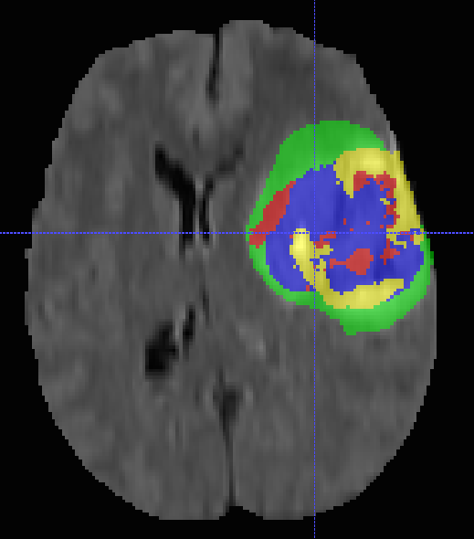
Fig. 19 depicts our results and those of the selected baselines on these three tasks. As before, the results clearly indicate that AL provides a significant improvement over passive selection. In this case we do not show all the variants of batch-mode query selection for the benefit of the figure clarity. Among the basic strategies, FMnMar gives the best performance in subtasks $1$ and $2$ and FMnMx in subtask $3$. Our entropy-based uncertainty strategies FEntS and FEntC perform better or equivalent to the corresponding baselines FMnMx and FMnMar as in the preliminary experiments. Next, the strategies with the geometric uncertainty CEnt, CEntS and CEntC outperform their corresponding FUn versions FEnt, FEntS and FEntC, where the improvement depends on the subtask and the strategy. Note that FEntS and FEntC as well as CEntS and CEntC perform equally well, thus, they can be used interchangeably. Further improvement is obtained when each of the strategies is combined with the optimal plane selection.

Figure 19: Comparison of different AL strategies for multi-class MRI segmentation. Dice scores for three BRATS2012 tasks: complete tumor, tumor core, enhancing tumor.

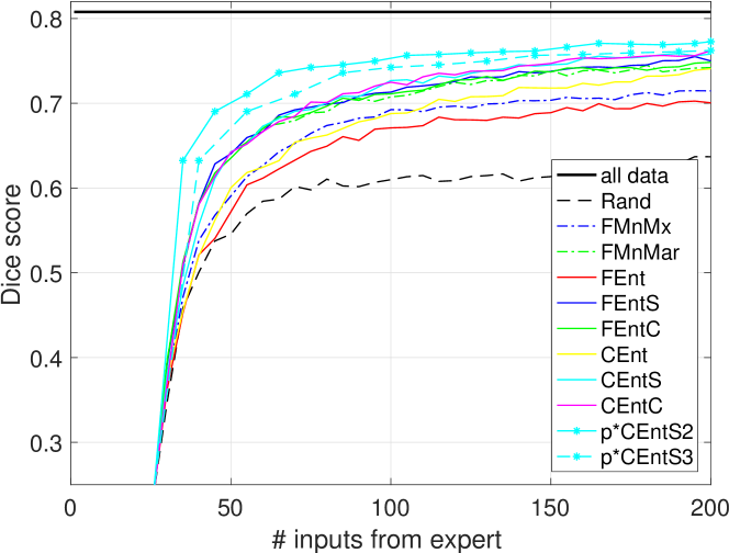
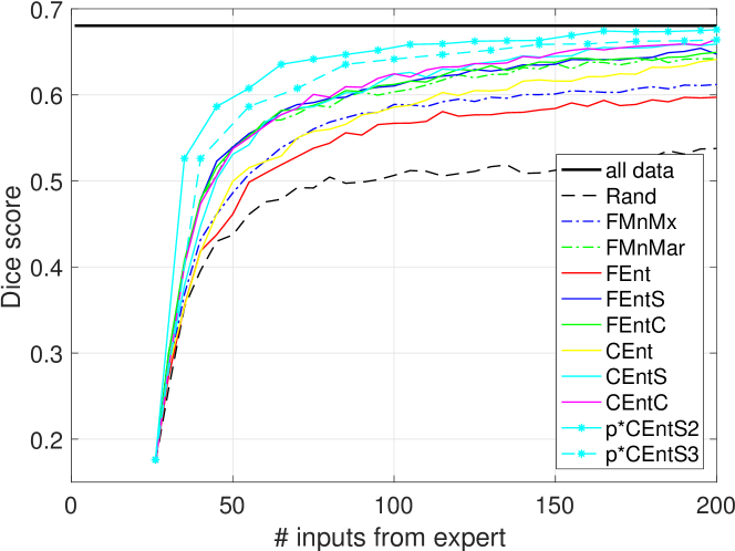
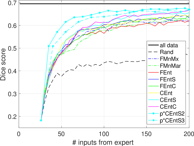
In practice, we observed that around $43$% of selected patches contain more than two classes. In such cases, simply finding a line separating two classes is not enough to annotate a patch. To handle such cases, we propose a different annotation scheme. The current prediction on supervoxels is displayed to the annotator who needs to correct the mistakes in the prediction. We count the number of misclassified samples throughout the experiments and on average there were no more than $10.42$% errors in the supervoxel classes, that is approximately $2.42$ supervoxels per iteration. Thus, we show the learning curves for the plane-based strategy and we count one annotation iteration as either two and or three inputs from the user, with both variants dominating non-batch selection.

Figure 20: Dice score for enhancing tumor segmentation. Performance of various strategies that have Selection Entropy at their basis.

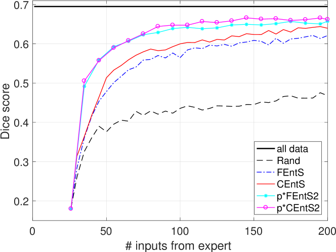
The difference between competing CUn strategies becomes negligible with a slight dominance of Selection Entropy p*CEntS in subtasks $1$ and $2$ and Total entropy p*CEnt in the last subtask. In seven of nine cases, the CUn in conjunction with the plane selection yields better results than FUn with plane selection and in two of nine, they perform equally well. For illustrative purposes, Fig. 19 contains only the best performing learning curve of p*CEntS and Fig. 20 shows the performance of all strategies based on the Selection Entropy in the third subtask.

6.6 Results on natural images

Finally, we turn to natural $2$D images and replace supervoxels by superpixels. In this case, the plane selection reduces to a simple selection of patches in the image and we will refer to these strategies as pFEnt and pCEnt because they do not involve the branch-and-bound selection procedure. In practice, we simply select superpixels with their $4$ neighbours in binary segmentation and $7$ in multi-class segmentation. This parameter is determined by the size of superpixels used in oversegmentation. Increasing this number would lead to higher learning rates in the same way as increasing the patch radius $r$, but we restrict it to a small value to ensure labelling of each patch can be done with little user intervention.

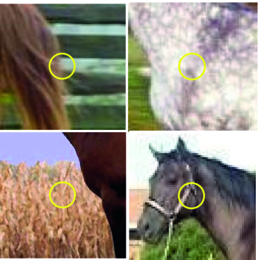
Foreground-background segmentation   We study the results of binary AL on the Weizmann horse database [70] in Fig. 21 and give the corresponding variances in Table I. To compute image features, we use Gaussian, Laplacian, Laplacian of Gaussian, Prewitt and Sobel filters for intensity and color values, gather first-order statistics such as local standard deviation, local range, gradient magnitude and direction histograms, as well as SIFT features. The pattern is again similar to the one observed in Figs. 15 and 17, with the difference between CEnt and pCEnt being smaller due to the fact that $2$D batch-mode approach does not involve any optimization of patch selection. Note, however, that while the first few iterations result in the reduced scores for all methods, plane-based methods are able to recover from this effect quite fast.

Figure 21: Comparison of various AL strategies for binary segmentation of natural images.

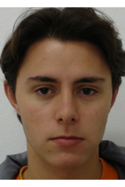
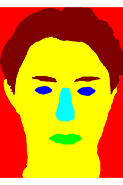
Multi-class face segmentation   We apply the multi-class AL to the task of segmenting human faces [71]. We distinguish $6$ classes: background, hair, skin, eyes, nose, and mouth. Fig. 22 demonstrates an example of an image from the dataset with the corresponding ground truth annotation. Notice again that we are dealing with unbalanced problem, obviously classes ‘eyes’, ‘nose’, ‘mouth’ are a minority compared to ‘background’, ‘skin’ and ‘hair’. We use the same features as for the Weizmann horse database plus HOG features.

(a)	(b)

Figure 22: Dataset for face segmentation (a) Example of an image from face segmentation dataset (b) Ground truth annotation for the given image. Different classes are indicated in different colors. Best viewed in color.

As in the case of multi-class MRI images, we must handle cases in which more than two classes are present in a single patch. However, this only happens in $0.84\%$ of the selected patches because three classes do no often co-occur in the same small neighborhood. Thus, we can still use the simple line separation heuristic depicted by Fig. 2 in most iterations and leave a user an opportunity to use a standard brush for rare refined annotations.

Figure 23: Comparing several AL strategies for multi-class face segmentation.

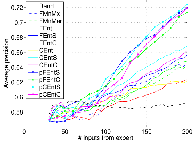
In Fig. 23 we compare our results to those of the baselines in terms of precision averaged over each one of the $6$ classes. This measure was chosen because it is better suited for capturing the performance in smaller classes and, thus reflects better the performance in segmentation with unbalanced classes. To ensure that performance on dominant classes is not sacrificed, we monitor the score of total precision (but omit the figure for conciseness), that shows similar performance for all AL strategies. Entropy-based algorithms FEntS and FEntC are better than the standard FMnMx and FMnMar, respectively. Moreover, selection that is based on the entropy allows for a combination with CUn and brings further improvement in average precision with the strategies CEnt, CEntS and CEntC. Next, each of the strategies can be used in conjunction with patch selection that allows for further improvement in the learning rate. We show the patch selection results only for Selection Entropy and Conditional Entropy and skip Total Entropy as it performs poorly in total precision. As we can see, the combination of plane selection with CUn strategies demonstrates better results at the end of learning experiments with the best result obtained by pCEntS.

6.7 Active learning or human intuition

Before we conclude the experiments, we would like to motivate why AL is important and why we cannot rely on human selecting the data for annotation manually. First advantage of AL is that it eliminates the cognitive cost for a human user who would otherwise need to decide which datapoint is informative for a classifier. For this, the human annotator would need to have a good understanding of the underlying classification algorithm. Besides, in the next experiment we show an example that demonstrates that not all human-intuitive strategies are useful for a classifier.

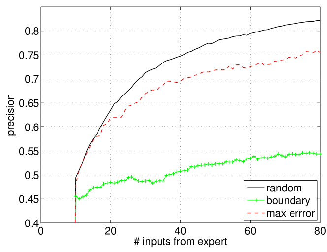
To design a human-intuitive selection strategy, we study distances to the closest class boundary for selected samples. For this purpose we count how many samples lie within radius of $10$ pixels from the boundary for $2$ strategies: Rand and CEntS in the face dataset. We observe that CEntS strategy samples $7.4$% more datapoints in this area than Rand. More superpixels in this area illustrate the effect of geometric component that prefers regions in the non-smooth areas of the prediction. Then, an intuitive strategy could be to first label patches at the boundary between classes. We implemented the selection strategies that simulate such user behaviours and we refer to it as boundary strategy.

To design another human-intuitive strategy, we notice that as part of the AL query selection procedure, we predict the segmentation for the whole training volume at every iteration. Given this prediction, a human expert could manually identify patches that are worth labelling. For example, he might first correct the most obvious mistakes. Thus, we simulate such a strategy max error by selecting first the most confidently but wrongly classified samples.

We ran fifty trials using each of these two strategies on the face segmentation problem of Sec. 6.6. Fig. 24 depicts the results. Surprisingly, the human strategies perform much worse than even passive data selection, that confirms the difficulty of the AL problem. The heuristics we proposed derive from our intuitive understanding of the problem. However, applying these intuitions is not straightforward for a human user. For example, it turns out that selecting samples that have the highest error leads to selecting outlier samples or those that have the most contradictory appearance. Thus, intelligent and automated query selection is necessary to determine how uncertain the classifier is and what smoothness prior should be used when selecting the next samples to be labelled.

Figure 24: Hypothetical human expert selection strategies. We demonstrate that strategies that are intuitive for a human annotator do not result in better performance than passive sampling.

7 Conclusion

In this paper we introduced an approach to exploit image geometry priors to increase the effectiveness of AL in image segmentation application. We propose entropy-based uncertainty measures for multi-class classification that can be combined with geometric priors in a principled way. In the segmentation of $2$D and $3$D images, our approach leverages the uncertainty information on the prediction at an image patch and at its neighbours. For $3$D image stacks, it adds an ability to select a $2$D planar patch where annotations are easier to perform. We demonstrate the effectiveness of our approach on several datasets featuring MRI, EM, and natural images and both for foreground-background and multi-class segmentation.

We conclude that intuitions about geometrical properties of images are useful to answer the question “What data to annotate?” in image segmentation. Besides, by reducing the annotation task from cumbersome $3$D annotations to $2$D annotations, we provide one possible answer to the question “How to annotate data?”. Moreover, we observe that addressing these two questions jointly can bring additional benefits to the annotation method. Finally, we notice that the human intuitions may not always result in a desirable behaviour.

Our hand-crafted annotation strategy brings us impressive cost savings in image segmentation. Yet, we realise that it would be impossible to design a selection strategy for every new problem at hand. Besides, our last experiment shows that not all human intuitions perform as expected. To overcome these limitation and systematically search in the space of possible strategies, in future work, we will strive to replace the heuristics we have introduced by AL strategies that are themselves learned and take into account image priors in annotation process.

References

- [1] A. Kovashka, O. Russakovsky, L. Fei-Fei, and K. Grauman, Crowdsourcing in Computer Vision. Foundations and Trends in Computer Graphics and Vision, 2016.
- [2] C. Long, G. Hua, and A. Kapoor, “Active visual recognition with expertise estimation in crowdsourcing,” in International Conference on Computer Vision, 2013.
- [3] T.-Y. Lin, M. Maire, S. Belongie, J. Hays, P. Perona, D. Ramanan, P. Dollár, and C. Zitnick, “Microsoft COCO: Common objects in context,” in European Conference on Computer Vision, 2014.
- [4] A. J. Joshi, F. Porikli, and N. P. Papanikolopoulos, “Scalable active learning for multiclass image classification,” IEEE Transactions on Pattern Analysis and Machine Intelligence, vol. 34, no. 11, pp. 2259–2273, 2012.
- [5] Q. Sun, A. Laddha, and D. Batra, “Active learning for structured probabilistic models with histogram approximation,” in Conference on Computer Vision and Pattern Recognition, 2015.
- [6] C. Käding, A. Freytag, E. Rodner, P. Bodesheim, and J. Denzler, “Active learning and discovery of object categories in the presence of unnameable instances,” in Conference on Computer Vision and Pattern Recognition, 2015.
- [7] W. H. Beluch, T. Genewein, A. Nürnberger, and J. M. Köhler, “The power of ensembles for active learning in image classification,” in Conference on Computer Vision and Pattern Recognition, 2018.
- [8] B. Schmid, J. Schindelin, A. Cardona, M. Longair, and M. Heisenberg, “A high-level 3D visualization API for Java and ImageJ,” BMC Bioinformatics, vol. 11, p. 274, 2010.
- [9] K. Konyushkova, R. Sznitman, and P. Fua, “Introducing geometry into active learning for image segmentation,” in International Conference on Computer Vision, 2015.
- [10] B. Settles, Active Learning. Morgan & Claypool Publishers, 2012.
- [11] D. D. Lewis and W. A. Gale, “A sequential algorithm for training text classifiers,” in ACM SIGIR proceedings on Research and Development in Information Retrieval, 1994.
- [12] W. Luo, A. G. Schwing, and R. Urtasun, “Latent structured active learning,” in Advances in Neural Information Processing Systems, 2013.
- [13] R. Gilad-Bachrach, A. Navot, and N. Tishby, “Query by committee made real,” in Advances in Neural Information Processing Systems, 2005.
- [14] A. Freytag, E. Rodner, and J. Denzler, “Selecting influential examples: Active learning with expected model output changes,” in European Conference on Computer Vision, 2014.
- [15] S. Hoi, R. Jin, J. Zhu, and M. Lyu, “Batch mode active learning and its application to medical image classification,” in International Conference on Machine Learning, 2006.
- [16] A. Kapoor, K. Grauman, R. Urtasun, and T. Darrell, “Active learning with gaussian processes for object categorization,” in International Conference on Computer Vision, 2007.
- [17] T. Luo, K. Kramer, S. Samson, A. Remsen, D. B. Goldgof, L. O. Hall, and T. Hopkins, “Active learning to recognize multiple types of plankton,” in International Conference on Pattern Recognition, 2004.
- [18] A. Joshi, F. Porikli, and N. Papanikolopoulos, “Multi-class active learning for image classification,” in Conference on Computer Vision and Pattern Recognition, 2009.
- [19] J. Long, E. Shelhamer, and T. Darrell, “Fully convolutional networks for semantic segmentation,” in Conference on Computer Vision and Pattern Recognition, 2015.
- [20] Y. Yang, Z. Ma, F. Nie, X. Chang, and A. G. Hauptmann, “Multi-class active learning by uncertainty sampling with diversity maximization,” International Journal of Computer Vision, vol. 113, no. 2, pp. 113–127, 2015.
- [21] P. Jain and A. Kapoor, “Active learning for large multi-class problems,” in Conference on Computer Vision and Pattern Recognition, 2009.
- [22] C. Körner and S. Wrobel, “Multi-class ensemble-based active learning,” in European Conference on Machine Learning, 2006, pp. 687–694.
- [23] K. Konyushkova, R. Sznitman, and P. Fua, “Learning active learning from real and synthetic data,” in Advances in Neural Information Processing Systems, 2017.
- [24] P. Bachman, A. Sordoni, and A. Trischler, “Learning algorithms for active learning,” in International Conference on Machine Learning, 2017.
- [25] B. Settles, “From theories to queries: Active learning in practice,” in Active Learning and Experimental Design Workshop in Conjunction with International Conference on Artificial Intelligence and Statistics, 2010.
- [26] L. Yang and J. Carbonell, “Buy-in-bulk active learning,” in Advances in Neural Information Processing Systems, 2013.
- [27] E. Elhamifar, G. Sapiro, A. Yang, and S. Sastry, “A convex optimization framework for active learning,” in International Conference on Computer Vision, 2013.
- [28] A. Al-Taie, H. H. K., and L. Linsen, “Uncertainty estimation and visualization in probabilistic segmentation,” Computers & Graphics, vol. 39, pp. 48–59, 2014.
- [29] M. Hasan and A. K. Roy-Chowdhury, “Context aware active learning of activity recognition models,” in International Conference on Computer Vision, 2015.
- [30] J. Johnson, L. Ballan, and L. Fei-Fei, “Love thy neighbors: Image annotation by exploiting image metadata,” in Conference on Computer Vision and Pattern Recognition, 2015.
- [31] A. Mosinska, R. Sznitman, P. Glowacki, and P. Fua, “Active learning for delineation of curvilinear structures,” in Conference on Computer Vision and Pattern Recognition, 2016.
- [32] M. Wigness, B. A. Draper, and J. R. Beveridge, “Efficient label collection for unlabeled image datasets,” in Conference on Computer Vision and Pattern Recognition, 2015.
- [33] C. Vondrick, D. Patterson, and D. Ramanan, “Efficiently scaling up crowdsourced video annotation,” International Journal of Computer Vision, vol. 101, pp. 184––204, 2013.
- [34] A. Vezhnevets, V. Ferrari, and J. Buhmann, “Weakly supervised structured output learning for semantic segmentation,” in Conference on Computer Vision and Pattern Recognition, 2012.
- [35] J. Iglesias, E. Konukoglu, A. Montillo, Z. Tu, and A. Criminisi, “Combining generative and discriminative models for semantic segmentation,” in Information Processing in Medical Imaging, 2011.
- [36] S. D. Jain and K. Grauman, “Active image segmentation propagation,” in Conference on Computer Vision and Pattern Recognition, 2016.
- [37] Q. Li, Z. Deng, Y. Zhang, X. Zhou, U. Nagerl, and S. Wong, “A global spatial similarity optimization scheme to track large numbers of dendritic spines in time-lapse confocal microscopy,” IEEE Transactions on Medical Imaging, vol. 30, no. 3, pp. 632–641, 2011.
- [38] D. Zhou, O. Bousquet, T. N. Lal, J. Weston, and B. Schölkopf, “Learning with local and global consistency,” in Advances in Neural Information Processing Systems, 2004.
- [39] B. Liu and V. Ferrari, “Active learning for human pose estimation,” in International Conference on Computer Vision, 2012.
- [40] S. M. Plaza, “Focused proofreading to reconstruct neural connectomes from EM images at scale,” in LABELS workshop at Conference on Medical Image Computing and Computer Assisted Intervention, 2016.
- [41] S. Paul, J. H. Bappy, and A. Roy-Chowdhury, “Non-uniform subset selection for active learning in structured data,” in Conference on Computer Vision and Pattern Recognition, 2017.
- [42] A. Zlateski, R. Jaroensri, P. Sharma, and F. Durand, “On the importance of label quality for semantic segmentation,” in Conference on Computer Vision and Pattern Recognition, 2018.
- [43] D. Lin, J. Dai, J. Jia, K. He, and J. Sun, “ScribbleSup: Scribble-supervised convolutional networks for semantic segmentation,” in Conference on Computer Vision and Pattern Recognition, 2016.
- [44] J. Xu, A. G. Schwing, and R. Urtasun, “Learning to segment under various forms of weak supervision,” in Conference on Computer Vision and Pattern Recognition, 2015.
- [45] N. S. Nagaraja, F. R. Schmidt, and T. Brox, “Video segmentation with just a few strokes,” in International Conference on Computer Vision, 2015.
- [46] A. Bearman, O. Russakovsky, V. Ferrari, and L. Fei-Fei, “What’s the point: Semantic segmentation with point supervision,” in European Conference on Computer Vision, 2016.
- [47] S. Bell, P. Upchurch, N. Snavely, and K. Bala, “Material recognition in the wild with the materials in context database,” in Conference on Computer Vision and Pattern Recognition, 2015.
- [48] T. Wang, B. Han, and J. Collomosse, “TouchCut: Fast image and video segmentation using single-touch interaction,” Computer Vision and Image Understanding, vol. 120, pp. 14–30, 2014.
- [49] S. D. Jain and K. Grauman, “Click carving: Segmenting objects in video with point clicks,” in Human Computation Workshop at American Association for Artificial Intelligence Conference, 2016.
- [50] L. Castrejon, K. Kundu, R. Urtasun, and S. Fidler, “Annotating object instances with a polygon-RNN,” in Conference on Computer Vision and Pattern Recognition, 2017.
- [51] D. Acuna, H. Ling, A. Kar, and S. Fidler, “Efficient interactive annotation of segmentation datasets with polygon-RNN++,” in Conference on Computer Vision and Pattern Recognition, 2018.
- [52] N. Gordillo, E. Montseny, and P. Sobrevilla, “State of the art survey on MRI brain tumor segmentation,” Magnetic Resonance in Medicine, vol. 31, no. 8, pp. 1426–1438, 2013.
- [53] A. Top, G. Hamarneh, and R. Abugharbieh, “Active learning for interactive 3D image segmentation,” in Conference on Medical Image Computing and Computer Assisted Intervention, 2011.
- [54] B. Andres, U. Koethe, M. Helmstaedter, W. Denk, and F. Hamprecht, “Segmentation of SBFSEM volume data of neural tissue by hierarchical classification,” in DAGM Symposium on Pattern Recognition, 2008, pp. 142–152.
- [55] A. Lucchi, K. Smith, R. Achanta, G. Knott, and P. Fua, “Supervoxel-based segmentation of mitochondria in EM image stacks with learned shape features,” IEEE Transactions on Medical Imaging, vol. 31, no. 2, pp. 474–486, February 2012.
- [56] R. Achanta, A. Shaji, K. Smith, A. Lucchi, P. Fua, and S. Suesstrunk, “SLIC superpixels compared to state-of-the-art superpixel methods,” IEEE Transactions on Pattern Analysis and Machine Intelligence, vol. 34, no. 11, pp. 2274–2282, November 2012.
- [57] L. Lovász, “Random walks on graphs: A survey,” in Combinatorics, Paul Erdos in Eighty, 1993.
- [58] L. Grady, “Random walks for image segmentation,” IEEE Transactions on Pattern Analysis and Machine Intelligence, vol. 28, no. 11, pp. 1768–1783, 2006.
- [59] C. Lampert, M. Blaschko, and T. Hofmann, “Beyond sliding windows: Object localization by efficient subwindow search,” in Conference on Computer Vision and Pattern Recognition, 2008.
- [60] R. Sznitman, C. Becker, F. Fleuret, and P. Fua, “Fast object detection with entropy-driven evaluation,” in Conference on Computer Vision and Pattern Recognition, 2013.
- [61] C. Becker, R. Rigamonti, V. Lepetit, and P. Fua, “Supervised feature learning for curvilinear structure segmentation,” in Conference on Medical Image Computing and Computer Assisted Intervention, September 2013.
- [62] C.-L. Liu, F. Yin, D.-H. Wang, and Q.-F. Wang, “Casia online and offline Chinese handwriting databases,” in Document Analysis and Recognition (ICDAR), 2011 International Conference on, 2011.
- [63] E. Johns, O. M. Aodha, and G. Brostow, “Becoming the expert - Interactive multi-class machine teaching,” in Conference on Computer Vision and Pattern Recognition, 2015.
- [64] Y. Jia, E. Shelhamer, J. Donahue, S. Karayev, J. Long, R. Girshick, S. Guadarrama, and T. Darrell, “Caffe: Convolutional architecture for fast feature embedding,” in ACM International Conference on Multimedia, 2014.
- [65] T. Hastie, R. Tibshirani, and J. Friedman, The Elements of Statistical Learning. Springer, 2001.
- [66] T. Pietzsch, S. Saalfeld, S. Preibisch, and P. Tomancak, “Bigdataviewer: visualization and processing for large image data sets,” Nature methods, vol. 12, no. 6, pp. 481–483, 2015.
- [67] M. Everingham, L. V. Gool, C. Williams, J. Winn, and A. Zisserman, “The Pascal visual object classes (voc) challenge,” International Journal of Computer Vision, vol. 88, no. 2, pp. 303–338, 2010.
- [68] G. Schohn and D. Cohn, “Less is more: Active learning with support vector machines,” in International Conference on Machine Learning, 2000.
- [69] B. Menza, A. Jacas et al., “The multimodal brain tumor image segmentation benchmark (BRATS),” IEEE Transactions on Medical Imaging, vol. 34, no. 10, pp. 1993 – 2024, 2014.
- [70] E. Borenstein and S. Ullman, “Combined top-down/bottom-up segmentation,” IEEE Transactions on Pattern Analysis and Machine Intelligence, vol. 30, no. 12, pp. 2109–2125, 2008.
- [71] K. Khan, M. Mauro, and R. Leonardi, “Multi-class semantic segmentation of faces,” in International Conference on Image Processing, 2015.