Distributed Stochastic Optimization for
Weakly Coupled Systems with Applications to Wireless Communications

Abstract

In this paper, a framework is proposed to simplify solving the infinite horizon average cost problem for the weakly coupled multi-dimensional systems. Specifically, to address the computational complexity issue, we first introduce a virtual continuous time system (VCTS) and obtain the associated fluid value function. The relationship between the VCTS and the original discrete time system is further established. To facilitate the low complexity distributed implementation and address the coupling challenge, we model the weakly coupled system as a perturbation of a decoupled base system and study the decoupled base system. The fluid value function of the VCTS is approximated by the sum of the per-flow fluid value functions and the approximation error is established using perturbation analysis. Finally, we obtain a low complexity distributed solution based on the per-flow fluid value function approximation. We apply the framework to solve a delay-optimal control problem for the $K$-pair interference networks and obtain a distributed power control algorithm. The proposed algorithm is compared with various baseline schemes through simulations and it is shown that significant delay performance gain can be achieved.

I Introduction

Stochastic optimization plays a key role in solving various optimal control problems under stochastic evolutions and it has a wide range of applications in multi-disciplinary areas such as control of complex computer networks [1], radio resource optimization in wireless systems [2] as well as financial engineering [3]. A common approach to solve stochastic optimization problems is via Markov Decision Process (MDP) [4], [5]. In the MDP approach, the state process evolves stochastically as a controlled Markov chain. The optimal control policy is obtained by solving the well-known Bellman equation. However, brute-force value iteration or policy iteration [6] cannot lead to viable solutions due to the curse of dimensionality. Specifically, the size of the state space and action space grows exponentially with the dimension of the state variables. The huge state space issue not only makes MDP problems intractable from computational complexity perspective but also has an exponentially large memory requirement for storing the value functions and policies. Furthermore, despite the complexity and storage issues, brute-force solution of MDP problems is also undesirable because it leads to centralized control, which induces huge signaling overhead in collecting the global system state information and broadcasting the overall control decisions at the controller.

To address the above issues, approximate dynamic programming (ADP) is proposed in [7, 8] to obtain approximate solutions to MDP problems. One approach in ADP is called state aggregation [9], [10], where the state space of the Markov chain is partitioned into disjoint regions. The states belonging to a partition region share the same control action and the same value function. Instead of finding solutions of the Bellman equation in the original huge state space, the controller solves a simpler problem in the aggregated state space (or reduced state space), ignoring irrelevant state information. While the size of the state space could be significantly reduced, it still involves solving a system of Bellman equations in the reduced state space, which is hard to deal with for large systems. Another approach in ADP is called basis function approximation [11], [12], i.e., approximating the value function by a linear combination of preselected basis functions. In such approximation architecture, the value function is computed by mapping it to a low dimensional function space spanned by the basis functions. In order to reduce the approximation error, proper weight associated with each basis function is then calculated by solving the projected Bellman equation [4]. Some existing works [13], [14] discussed the basis function adaptation problem where the basis functions are parameterized and their parameters are tuned by minimizing an objective function according to some evaluation criteria (e.g., Bellman error). State aggregation technique can be viewed as a special case of the basis function approximation technique [15], where the basis function space is determined accordingly when a method of constructing an aggregated state space is given. Both approaches can be used to solve MDP problems for systems with general dynamic structures but they fail to exploit the potential problem structures and it is also non-trivial to apply these techniques to obtain distributed solutions.

In this paper, we are interested in distributed stochastic optimization for multi-dimensional systems with weakly coupled dynamics in control variables. Specifically, there are $K$ control agents in the system with $K$ sub-system state variables $(\mathbf{x}_{1},\dots,\mathbf{x}_{K})$. The evolution of the $k$-th sub-system state $\mathbf{x}_{k}$ is weakly affected by the control actions of the $j$-th agent for all $j\neq k$. To solve the stochastic optimization problem, we first construct a virtual continuous time system (VCTS) using the fluid limit approximation approach. The Hamilton-Jacobi-Bellman (HJB) equation associated with the optimal control problem of the VCTS is closely related to the Bellman equation associated with the optimal control problem of the original discrete time system (ODTS). Note that although the VCTS approach is related to the fluid limit approximation approach as discussed in [1], [16]–[20], there is a subtle difference between them. For instance, the fluid limit approximation approach is based on the functional law of large numbers [21] for the state dynamic evolution while the proposed VCTS approach is based on problem transformation. In order to obtain a viable solution for the multi-dimensional systems with weakly coupled dynamics, there are several first order technical challenges that need to be addressed.

• Challenges due to the Coupled State Dynamics and Distributed Solutions: For multi-dimensional systems with coupled state dynamics, the HJB equation associated with the VCTS is a multi-dimensional partial differential equation (PDE), which is quite challenging in general. Furthermore, despite the complexity issue involved, the solution structure requires centralized implementation, which is undesirable from both signaling and computational perspectives. There are some existing works using the fluid limit approximation approach to solve MDP problems [16]–[18] but they focus mostly on single dimensional problems [16] or centralized solutions for multi-dimensional problems in large scale networks [17, 18]. It is highly non-trivial to apply these existing fluid techniques to derive distributed solutions.

• Challenges on the Error-Bound between the VCTS and the ODTS: It is well-known that the fluid value function is closely related to the relative value function of the discrete time system. For example, for single dimensional systems [16] or heavily congested networks with centralized control [17, 19], the fluid value function is a useful approximator for the relative value function of the ODTS. Furthermore, the error bound between the fluid value function and the relative value function is shown to be $O(\|\mathbf{x}\|^{2})$ for large state $\mathbf{x}$ [1, 18]. However, extending these results to the multi-dimensional systems with distributed control policies is highly non-trivial.

• Challenges due to the Non-Linear Per-Stage Cost in Control Variables: There are a number of existing works using fluid limit approximation to solve MDP problems [16]–[20]. However, most of the related works only considered linear cost function [17]–[19] and relied on the exact closed-form solution of the associated fluid value function [16], [20]. Yet, in many applications, such as wireless communications, the data rate is a highly non-linear function of the transmit power and these existing results based on the closed-form fluid limit approximation cannot be directly applied to the general case with non-linear per-stage cost in control variables.

In this paper, we shall focus on distributed stochastic optimization for multi-dimensional systems with weakly coupled dynamics. We consider an infinite horizon average cost stochastic optimization problem with general non-linear per-stage cost function. We first introduce a VCTS to transform the original discrete time average cost optimization problem into a continuous time total cost problem. The motivation of solving the problem in the continuous time domain is to leverage the well-established mathematical tools from calculus and differential equations. By solving the HJB equation associated with the total cost problem for the VCTS, we obtain the fluid value function, which can be used to approximate the relative value function of the ODTS. We then establish the relationship between the fluid value function of the VCTS and the relative value function of the discrete time system. To address the low complexity distributed solution requirement and the coupling challenge, the weakly coupled system can be modeled as a perturbation of a decoupled base system. The solution to the stochastic optimization problem for the weakly coupled system can be expressed as solutions of $K$ distributed per-flow HJB Equations. By solving the per-flow HJB equation, we obtain the per-flow fluid value function, which can be used to generate localized control actions at each agent based on locally observable system states. Using perturbation analysis, we establish the gap between the fluid value function of the VCTS and the sum of the per-flow fluid value functions. Finally, we show that solving the Bellman equation associated with the original stochastic optimization problem using per-flow fluid value function approximation is equivalent to solving a deterministic network utility maximization (NUM) problem [22], [23] and we propose a distributed algorithm for solving the associated NUM problem. We shall illustrate the above framework of distributed stochastic optimization using an application example in wireless communications. In the example, we consider the delay optimal control problem for $K$-pair interference networks, where the queue state evolution of each transmitter is weakly affected by the control actions of the other transmitters due to the cross-channel interference. The delay performance of the proposed distributed solution is compared with various baseline schemes through simulations and it is shown that substantial delay performance gain can be achieved.

II System Model and Problem Formulation

In this section, we elaborate on the weakly coupled multi-dimensional systems. We then formulate the associated infinite horizon average cost stochastic optimization problem and discuss the general solution. We illustrate the application of the framework using an application example in wireless communications.

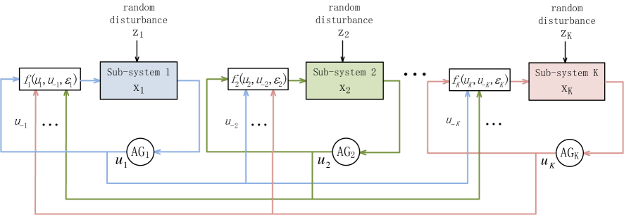
Figure 1: System model of a $K$-dimensional multi-agent control system. $\text{AG}_{k}$ is the control agent associated with the $k$-th sub-system.

II-A Multi-Agent Control System with Weakly Coupled Dynamics

We consider a multi-dimensional system with weakly coupled dynamics as shown in Fig. 1. The system consists of $K$ control agents indexed by $k\in\mathcal{K}$, where $\mathcal{K}=\{1,\dots,K\}$. The time dimension is discretized into decision epochs indexed by $t$ with epoch duration $\Delta$. The weakly coupled multi-agent control system is a time-homogeneous MDP model which can be characterized by four elements, namely the state space, the action space, the state transition kernel and the system cost. We elaborate on the multi-agent control system as follows.

The global system state $\mathbf{x}\left(t\right)=\left(\mathbf{x}_{1}\left(t\right),\dots,\mathbf{x}_{K}\left(t\right)\right)\in\boldsymbol{\mathcal{X}}\triangleq\mathcal{X}_{1}\times\dots\times\mathcal{X}_{K}$ at the $t$-th epoch is partitioned into $K$ sub-system states, where $\mathbf{x}_{k}\left(t\right)\in\mathcal{X}_{k}$ denote the $k$-th sub-system state at the $t$-th epoch. $\boldsymbol{\mathcal{X}}$ and $\mathcal{X}_{k}$ are the global system state space and sub-system state space, respectively. The $k$-th control agent generates a set of control actions $\mathbf{u}_{k}\left(t\right)\in\mathcal{U}_{k}$ at the $t$-th epoch, where $\mathcal{U}_{k}$ is a compact action space for the $k$-th sub-system. Furthermore, we denote $\mathbf{u}\left(t\right)=\left(\mathbf{u}_{1}\left(t\right),\dots,\mathbf{u}_{K}\left(t\right)\right)\in\boldsymbol{\mathcal{U}}\triangleq\mathcal{U}_{1}\times\dots\times\mathcal{U}_{K}$ as the global control action, where $\boldsymbol{\mathcal{U}}$ is the global action space. Given an initial global system state $\mathbf{x}(0)\in\boldsymbol{\mathcal{X}}$, the $k$-th sub-system state $\mathbf{x}_{k}\left(t\right)$ evolves according to the following dynamics:

$$\mathbf{x}_{k}(t+1)=\mathbf{x}_{k}\left(t\right)+\mathbf{f}_{k}\left(\mathbf{u}_{k}\left(t\right),\mathbf{u}_{-k}\left(t\right),\boldsymbol{\epsilon}_{k}\right)\Delta+\mathbf{z}_{k}\left(t\right)\Delta,\quad\mathbf{x}_{k}(0)\in\mathcal{X}_{k}$$ (1)

where $\mathbf{u}_{-k}\left(t\right)=\{\mathbf{u}_{j}\left(t\right):\forall j\neq k\}$ and $\boldsymbol{\epsilon}_{k}=\{\epsilon_{kj}:\forall j\neq k\}$. $\epsilon_{kj}$ ($k\neq j$) is the coupling parameter that measures the extent to which the control actions of the $j$-th agent affect the state evolution of the $k$-th sub-system. In this paper, we assume that $\mathbf{f}_{k}\left(\mathbf{u}_{k}\left(t\right),\mathbf{u}_{-k}\left(t\right),\boldsymbol{\epsilon}_{k}\right)$ has the form $\mathbf{f}_{k}\left(\mathbf{u}_{k}\left(t\right),\epsilon_{k,1}\mathbf{u}_{1}\left(t\right),\cdots,\epsilon_{k,k-1}\mathbf{u}_{k-1}\left(t\right),\right.\\ \left.\epsilon_{k,k+1}\mathbf{u}_{k+1}\left(t\right),\cdots,\epsilon_{k,K}\mathbf{u}_{K}\left(t\right)\right)$, and $\mathbf{f}_{k}\left(\mathbf{u}_{k},\mathbf{u}_{-k},\boldsymbol{\epsilon}_{k}\right)$ is continuously differentiable w.r.t. each element in $\mathbf{u}_{k}$, $\mathbf{u}_{-k}$ and $\boldsymbol{\epsilon}_{k}$. $\mathbf{z}_{k}\in\boldsymbol{\mathcal{Z}}$ is a random disturbance process for the $k$-th sub-system, where $\boldsymbol{\mathcal{Z}}$ is the disturbance space. We have the following assumption on the disturbance process.

Assumption 1 (Disturbance Process Model).

The disturbance process $\mathbf{z}_{k}\left(t\right)$ is i.i.d. over decision epochs according to a general distribution $\Pr[\mathbf{z}_{k}]$ with finite mean $\mathbb{E}[\mathbf{z}_{k}]=\overline{\mathbf{z}}_{k}$ for all $k\in\mathcal{K}$. Furthermore, the disturbance processes $\{\mathbf{z}_{k}\left(t\right)\}$ are independent w.r.t. $k$.  ∎

Given the global system state $\mathbf{x}\left(t\right)$ and the global control action $\mathbf{u}\left(t\right)$ at the $t$-th epoch, the system evolves as a controlled Markov chain according to the following transition kernel:

$$\Pr[\mathbf{x}(t+1)\in A|\mathbf{x}\left(t\right),\mathbf{u}\left(t\right)]=\prod_{k}\underbrace{\Pr[\mathbf{x}_{k}(t+1)\in A_{k}|\mathbf{x}_{k}\left(t\right),\mathbf{u}\left(t\right)]}_{\text{transition kernel of the $k$-th sub-system}}$$

$$= \prod_{k}\Pr[\mathbf{x}_{k}\left(t\right)+\mathbf{f}_{k}\left(\mathbf{u}_{k}\left(t\right),\mathbf{u}_{-k}\left(t\right),\boldsymbol{\epsilon}_{k}\right)\Delta+\mathbf{z}_{k}\left(t\right)\Delta\in A_{k}]$$ (2)

where $A=\otimes_{k=1}^{K}A_{k}$ is a measurable set with $A_{k}\in\mathcal{X}_{k}$ for all $k\in\mathcal{K}$. Note that the transition kernel in (2) is time-homogeneous.

We consider a system cost function $c:\boldsymbol{\mathcal{X}}\times\boldsymbol{\mathcal{U}}\rightarrow[0,\infty]$ given by

$$c(\mathbf{x},\mathbf{u})=\sum_{k=1}^{K}c_{k}(\mathbf{x}_{k},\mathbf{u}_{k})$$ (3)

where $c_{k}:\mathcal{X}_{k}\times\mathcal{U}_{n}\rightarrow[0,\infty)$ is the cost function of the $k$-th sub-system given by

$$c_{k}(\mathbf{x}_{k},\mathbf{u}_{k})=\alpha_{k}\|\mathbf{x}_{k}\|_{\mathbf{v}_{k},1}+g_{k}\left(\mathbf{u}_{k}\right)$$ (4)

where $\alpha_{k}$ is some positive constant, $\|\cdot\|_{\mathbf{v}_{k},1}$ is a weighted $\mathcal{L}_{1}$ norm with $\mathbf{v}_{k}$ being the corresponding weight vector and $g_{k}$ is a continuously differentiable function w.r.t. each element in vector $\mathbf{u}_{k}$. In addition, we assume $\left|g_{k}\left(\mathbf{u}_{k}\right)\right|<\infty$ for all $\mathbf{u}_{k}\in\mathcal{U}_{k}$.

Definition 1 (Decoupled and Weakly Coupled Systems).

A multi-dimensional system in (1) is called decoupled if all the coupling parameters are equal to zero. A multi-dimensional system in (1) is called weakly coupled if all the coupling parameters $\{\epsilon_{kj}:\forall k,j\in\mathcal{K},k\neq j\}$ are very small. For weakly coupled systems, the state dynamics of each sub-system is weakly affected by the control actions of the other sub-systems as shown in the state evolution equation in (1). In addition, define $\epsilon=\max\left\{\left|\epsilon_{kj}\right|:\forall k,j\in\mathcal{K},k\neq j\right\}$. Then, we have $|\epsilon_{kj}|\leq\epsilon$ for all $k,j\in\mathcal{K},k\neq j$.  ∎

Note that the above framework considers the coupling due to the control actions only. Yet, it has already covered many examples in wireless communications such as the interference networks with weak interfering cross links and the multi-user MIMO broadcast channels with perturbated channel state information. We shall illustrate the application of the framework using interference networks as an example in Section II-C.

II-B Control Policy and Problem Formulation

In this subsection, we introduce the stationary centralized control policy and formulate the infinite horizon average cost stochastic optimization problem.

Definition 2 (Stationary Centralized Control Policy).

A stationary centralized control policy of the $k$-th sub-system $\Omega_{k}:\boldsymbol{\mathcal{X}}\rightarrow\mathcal{U}_{k}$ is defined as a mapping from the global system state space $\boldsymbol{\mathcal{X}}$ to the action space of the $k$-th sub-system $\mathcal{U}_{k}$. Given a global system state realization $\mathbf{x}\in\boldsymbol{\mathcal{X}}$, the control action of the $k$-th sub-system is given by $\Omega_{k}\left(\mathbf{x}\right)=\mathbf{u}_{k}\in\mathcal{U}_{k}$. Furthermore, let $\Omega=\{\Omega_{k}:\forall k\}$ denote the aggregation of the control policies for all the $K$ sub-systems.  ∎

Assumption 2 (Admissible Control Policy).

A policy $\Omega$ is assumed to be admissible if the following requirements are satisfied:

• it is unichain, i.e., the controlled Markov chain $\left\{\mathbf{x}\left(t\right)\right\}$ has a single recurrent class (and possibly some transient states) [4].

• it is $n$-th order stable, i.e., $\lim_{T\rightarrow\infty}\mathbb{E}^{\Omega}\left[\left|\mathbf{Q}\right|^{n}\right]<\infty$.

• $\mathbf{u}=\Omega(\mathbf{x})$ satisfies some constraints depending on the different application scenarios.  ∎

Given an admissible control policy $\Omega$, the average cost of the system starting from a given initial global system state $\mathbf{x}\left(0\right)$ is given by

$$\overline{L}^{\Omega}\left(\mathbf{x}\left(0\right)\right)=\limsup_{T\rightarrow\infty}\frac{1}{T}\sum_{t=0}^{T-1}\mathbb{E}^{\Omega}[c(\mathbf{x}\left(t\right),\Omega(\mathbf{x}\left(t\right)))]$$ (5)

where $\mathbb{E}^{\Omega}$ means taking expectation w.r.t. the probability measure induced by the control policy $\Omega$.

We consider an infinite horizon average cost problem. The objective is to find an optimal policy such that the average cost in (5) is minimized. Specifically, we have:

Problem 1 (Infinite Horizon Average Cost Problem).

The infinite horizon average cost problem for the multi-agent control system is formulated as follows:

$$\min_{\Omega}\overline{L}^{\Omega}\left(\mathbf{x}\left(0\right)\right)$$ (6)

where $\overline{L}^{\Omega}\left(\mathbf{x}\left(0\right)\right)$ is given in (5).   ∎

Under the assumption of the admissible control policy, the optimal control policy of Problem 1 is independent of the initial state $\mathbf{x}\left(0\right)$ and can be obtained by solving the Bellman equation [4], which is summarized in the following lemma:

Lemma 1 (Sufficient Conditions for Optimality under ODTS).

If there exists a ($\theta^{\ast},\{V\left(\mathbf{x}\right)\}$) that satisfies the following Bellman equation:

$$\theta^{\ast}\Delta+V\left(\mathbf{x}\right)=\min_{\Omega\left(\mathbf{x}\right)}\left[c\left(\mathbf{x},\Omega\left(\mathbf{x}\right)\right)\Delta+\left(\mathrm{\Gamma}_{\Omega}V\right)\left(\mathbf{x}\right)\right],\quad\forall\mathbf{x}\in\boldsymbol{\mathcal{X}}$$ (7)

where the operator $\Gamma_{\Omega}$ on $V\left(\mathbf{x}\right)$ is defined as $(\Gamma_{\Omega}V)\left(\mathbf{x}\right)=\mathbb{E}\left[V\left(\mathbf{x}\left(t+1\right)\right)\big{|}\mathbf{x}\left(t\right)=\mathbf{x},\Omega\left(\mathbf{x}\right)\right]$. Suppose for all admissible control policy $\Omega$ and initial global system state $\mathbf{x}\left(0\right)$, the following transversality condition is satisfied:

$$\lim_{T\rightarrow\infty}\frac{1}{T}\big{[}V\left(\mathbf{x}\left(0\right)\right)-\mathbb{E}\left[V\left(\mathbf{x}\left(T\right)\right)|\mathbf{x}\left(0\right),\left\{\Omega(\mathbf{x}\left(t\right)):0\leq t\leq T\right\}\right]\big{]}=0$$ (8)

Then $\theta^{\ast}=\overline{L}^{\ast}=\min_{\Omega}\overline{L}(\Omega)$ is the optimal average cost. If $\Omega^{\ast}\left(\mathbf{x}\right)$ attains the minimum of the R.H.S. of (7) for all $\mathbf{x}\in\boldsymbol{\mathcal{X}}$, $\Omega^{\ast}$ is the optimal control policy. $V\left(\mathbf{x}\right)$ is called the relative value function.  ∎

Proof.

Please refer to [4] for details. ∎

Based on Lemma 1, we establish the following corollary on the approximate optimal solution.

Corollary 1 (Approximate Optimal Solution).

If there exists a ($\tilde{\theta}^{\ast},\{\widetilde{V}\left(\mathbf{x}\right)\}$) that satisfies the following approximate Bellman equation:

$$\tilde{\theta}^{\ast}=\min_{\Omega\left(\mathbf{x}\right)}\left[c\left(\mathbf{x},\Omega\left(\mathbf{x}\right)\right)+\nabla_{\mathbf{x}}V\left(\mathbf{x}\right)\left[\mathbf{f}\left(\Omega\left(\mathbf{x}\right),\boldsymbol{\epsilon}\right)+\overline{\mathbf{z}}\right]^{T}\right],\quad\forall\mathbf{x}\in\boldsymbol{\mathcal{X}}$$ (9)

where $\nabla_{\mathbf{x}}\widetilde{V}\left(\mathbf{x}\right)\triangleq\left(\nabla_{\mathbf{x}_{1}}\widetilde{V}\left(\mathbf{x}\right),\dots,\nabla_{\mathbf{x}_{K}}\widetilde{V}\left(\mathbf{x}\right)\right)$, $\mathbf{f}\left(\mathbf{u},\boldsymbol{\epsilon}\right)\triangleq\left(\mathbf{f}_{1}\left(\mathbf{u}_{1},\mathbf{u}_{-1},\boldsymbol{\epsilon}_{1}\right),\dots,\mathbf{f}_{K}\left(\mathbf{u}_{K},\mathbf{u}_{-K},\boldsymbol{\epsilon}_{K}\right)\right)$, $\overline{\mathbf{z}}=\left(\overline{\mathbf{z}}_{1},\dots,\overline{\mathbf{z}}_{K}\right)$ and $\boldsymbol{\epsilon}\triangleq\left\{\boldsymbol{\epsilon}_{k}:\forall k\right\}$. Suppose for all admissible control policy $\Omega$ and initial global system state $\mathbf{x}\left(0\right)$, the transversality condition in (8) is satisfied. Then,

$$\theta^{\ast} =\tilde{\theta}^{\ast}+\mathcal{O}\left(\Delta\right)$$ (10)

$$V\left(\mathbf{x}\right) =\widetilde{V}\left(\mathbf{x}\right)+\mathcal{O}\left(\Delta\right)$$ (11)

∎

Proof.

Please refer to Appendix A. ∎

Deriving the optimal control policy from (7) (or from (9)) requires the knowledge of the relative value function $\{V\left(\mathbf{x}\right)\}$. However, obtaining the relative value function is not trivial as it involves solving a large system of nonlinear fixed point equations. Brute-force approaches such as value iteration or policy iteration [4] require huge complexity and cannot lead to any implementable solutions. Furthermore, deriving the optimal control policy $\Omega^{\ast}$ requires knowledge of the global system state, which is undesirable from the signaling loading perspective. We shall obtain low complexity distributed solutions using the virtual continuous time system (VCTS) approach in Section III.

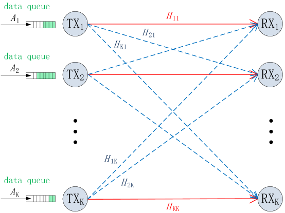
Figure 2: System model of a K-pair interference network. Each transmitter maintains a data queue for the bursty traffic flow towards the desired receiver in the network.

II-C Application Example – K–Pair Interference Networks

In this subsection, we illustrate the application of the above multi-agent control framework using interference networks as an example. We consider a $K$-pair interference network as illustrated in Fig. 2. The $k$-th transmitter sends information to the $k$-th receiver and all the $K$ transmitter-receiver (Tx-Rx) pairs share the same spectrum (and hence, they potentially interfere with each other). The received signal at the $k$-th receiver is given by

$$r_{k}=\sqrt{L_{kk}}H_{kk}s_{k}+\sum_{j\neq k}\sqrt{L_{kj}}H_{kj}s_{j}+z_{k}$$ (12)

where $L_{kj}$ and $H_{kj}$ are the long term path gain and microscopic fading coefficient from the $j$-th transmitter to the $k$-th receiver, respectively. $H_{kj}$ follows a complex Gaussian distribution with unit variance, i.e., $H_{kj}\sim\mathcal{CN}(0,1)$. $s_{k}$ is the symbol sent by the $k$-th transmitter, and $z_{k}\sim\mathcal{CN}(0,1)$ is i.i.d. complex Gaussian channel noise. Each Tx-Rx pair in Fig. 2 corresponds to one sub-system according to the general model in Section II-A. The $k$-th transmitter in this example corresponds to the $k$-th control agent in the general model. Denote the global CSI (microscopic fading coefficient) as $\mathbf{H}=\{H_{kj}:\forall k,j\in\mathcal{K}\}$. The time dimension is partitioned into decision epochs indexed by $t$ with duration $\tau$. We have the following assumption on the channel model.

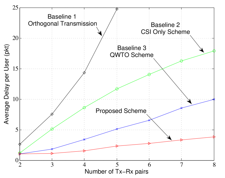
Figure 3: Illustration of the decision epochs, time slots and the associated arrival and departure events in the application example. $\mathbf{A}\left(t\right)$ is the random packet arrival at the beginning of the $(t+1)$-th decision epoch. The decision epoch is divided into equal-sized time slots with i.i.d. microscopic fading coefficient $\mathbf{H}_{1},\dots,\mathbf{H}_{N}$. $\mathbf{R}\left(t\right)=\left(R_{1}\left(t\right),\dots,R_{K}\left(t\right)\right)$ is the controlled global departure process at the end of the $t$-th epoch, where $R_{k}\left(t\right)$ is the average rate (averaged over $\mathbf{H}$) of the $k$-th Tx-Rx pair given in (13).

Assumption 3 (Channel Model).

We assume fast fading on the microscopic fading coefficient $\mathbf{H}$. The decision epoch is divided into equal-sized time slots as shown in Fig. 3. The slot duration is sufficiently small compared with $\tau$. $H_{kj}\left(t\right)$ remains constant within each slot and is i.i.d. over slots. Furthermore, $\left\{H_{kj}\left(t\right)\right\}$ is independent w.r.t. $\left\{k,j\right\}$. The path gain $\{L_{kj}:\forall k,j\in\mathcal{K}\}$ remains constant for the duration of the communication session.   ∎

There is a bursty data source at each transmitter and let $\mathbf{A}\left(t\right)=\left(A_{1}\left(t\right),\dots,A_{K}\left(t\right)\right)$ be the random new arrivals (number of packets per second) for the $K$ transmitters at the beginning of the $(t+1)$-th epoch. We have the following assumption on the arrival process.

Assumption 4 (Bursty Source Model).

The arrival process $A_{k}\left(t\right)$ is i.i.d. over decision epochs according to a general distribution $\Pr(A_{k})$ with finite average arrival rate $\mathbb{E}[A_{k}]=\lambda_{k}$ for all $k\in\mathcal{K}$. Furthermore, the arrival process $\{A_{k}\left(t\right)\}$ is independent w.r.t. $k$.  ∎

Let $\mathbf{Q}\left(t\right)=\left(Q_{1}\left(t\right),\dots,Q_{K}\left(t\right)\right)\in\boldsymbol{\mathcal{Q}}\triangleq\mathcal{Q}^{K}$ denote the global queue state information (QSI) at the beginning of the $t$-th epoch, where $Q_{k}\left(t\right)\in\mathcal{Q}$ is the local QSI denoting the number of packets (pkts) at the data queue for the $k$-th transmitter and $\mathcal{Q}$ is the local QSI state space of each transmitter. $Q_{k}\left(t\right)$ corresponds to the state of the $k$-th sub-system in the general model in Section II-A.

Treating interference as noise, the ergodic capacity (pkts/second) of the $k$-th Tx-Rx pair at the $t$-th epoch is given by

$$R_{k}\left(\mathbf{p}\left(t\right)\right)=\mathbb{E}\left[\log\left(1+\frac{p_{k}^{\mathbf{H}}\left(t\right)L_{kk}|H_{kk}|^{2}}{1+\sum_{j\neq k}p_{j}^{\mathbf{H}}\left(t\right)L_{kj}|H_{kj}|^{2}}\right)\bigg{|}\mathbf{Q}\left(t\right)\right]$$ (13)

where $\mathbb{E}[\cdot|\mathbf{Q}\left(t\right)]$ denotes the conditional expectation given $\mathbf{Q}\left(t\right)$, and $p_{k}^{\mathbf{H}}\left(t\right)$ is the transmit power of the $k$-th transmitter at the $t$-th epoch when the global CSI realization is $\mathbf{H}$. Since the transmitter cannot transmit more than $Q_{k}\left(t\right)$ at any decision epoch $t$, we require $R_{k}\left(t\right)\tau\leq Q_{k}\left(t\right)$, i.e.,

$$\mathbb{E}\left[\log\left(1+\frac{p_{k}^{\mathbf{H}}\left(t\right)L_{kk}|H_{kk}|^{2}}{1+\sum_{j\neq k}p_{j}^{\mathbf{H}}\left(t\right)L_{kj}|H_{kj}|^{2}}\right)\bigg{|}\mathbf{Q}\left(t\right)\right]\tau\leq Q_{k}\left(t\right)$$ (14)

Hence, the queue dynamics for the $k$-th transmitter is given by

$$Q_{k}(t+1) =Q_{k}\left(t\right)-R_{k}\left(t\right)\tau+A_{k}\left(t\right)\tau$$ (15)

The time epochs for the arrival and departure events of the global system are illustrated in Fig. 3.

Comparing with the state dynamics of the general system framework in (1), we have $\Delta=\tau$, $\mathbf{f}_{k}\left(\mathbf{u}_{k}\left(t\right),\mathbf{u}_{-k}\left(t\right),{\boldsymbol{\epsilon}}_{k}\right)=-R_{k}\left(t\right)\tau=-\mathbb{E}\left[\log\left(1+\frac{p_{k}^{\mathbf{H}}\left(t\right)L_{kk}|H_{kk}|^{2}}{1+\sum_{j\neq k}p_{j}^{\mathbf{H}}\left(t\right)L_{kj}|H_{kj}|^{2}}\right)\bigg{|}\mathbf{Q}\left(t\right)\right]\tau$, $\epsilon_{kj}=L_{kj}$ and $\mathbf{z}_{k}\left(t\right)=A_{k}\left(t\right)$ in the example. The control action generated by the $k$-th control agent ($k$-th transmitter) is $\mathbf{u}_{k}\left(t\right)=\mathbf{p}_{k}\left(t\right)=\{p_{k}^{\mathbf{H}}\left(t\right):\forall\mathbf{H}\}$. Furthermore, we have $\mathbf{u}_{-k}\left(t\right)=\boldsymbol{\mathbf{p}}_{-k}\left(t\right)=\{p_{j}^{\mathbf{H}}\left(t\right):\forall\mathbf{H},j\neq k\}$, and $\boldsymbol{\epsilon}_{k}=\mathbf{L}_{k}\triangleq\left\{L_{kj}:\forall j\neq k\right\}$. Define $L=\max\{L_{kj}:\forall k,j\in\mathcal{K},k\neq j\}$, then we have $L_{kj}\leq L$ for all $k,j\in\mathcal{K},k\neq j$. This corresponds to a physical interference network with weak interfering cross links due to the small cross-channel path gain. For simplicity, let $\boldsymbol{\mathbf{p}}\left(t\right)=\{\mathbf{p}_{k}\left(t\right):\forall k\}$ be the collection of power control actions of all the $K$ transmitters. We define the system cost function as

$$c\left(\mathbf{Q},\boldsymbol{\mathbf{p}}\right)=\sum_{k=1}^{K}c_{k}(Q_{k},\mathbf{p}_{k})$$ (16)

where $c_{k}(Q_{k},\mathbf{p}_{k})$ is the cost function of the $k$-th Tx-Rx pair which is given by

$$c_{k}(Q_{k},\mathbf{p}_{k})=\beta_{k}\frac{Q_{k}}{\lambda_{k}}+\gamma_{k}\mathbb{E}[p_{k}^{\mathbf{H}}|\mathbf{Q}]$$ (17)

where $\beta_{k}>0$ is a positive weight of the delay cost and $\gamma_{k}>0$ is the Lagrangian weight of the transmit power cost of the $k$-th transmitter.

The $K$-pair interference network with small cross-channel path gain is a weakly coupled multi-dimensional system according to Definition 1. The specific association with the general model in Section II-A is summarized in Table I.

Multi-agent control systems	K-pair interference networks
control agent	transmitter
sub-system	Tx-Rx pair
$\Delta$	$\tau$
$\mathbf{x}$	$\mathbf{Q}$
$\mathbf{x}_{k}$	$Q_{k}$
$\epsilon_{kj}$	$L_{kj}$
$\mathbf{u}$	$\boldsymbol{\mathbf{p}}$
$\mathbf{u}_{k}$	$\mathbf{p}_{k}$
$\mathbf{u}_{-k}$	$\boldsymbol{\mathbf{p}}_{-k}$
$\boldsymbol{\epsilon}_{k}$	$\mathbf{L}_{k}$
$\mathbf{z}_{k}$	$A_{k}$
$\mathbf{f}_{k}\left(\mathbf{u}_{k}\left(t\right),\mathbf{u}_{-k}\left(t\right),\boldsymbol{\epsilon}_{k}\right)$	$-\mathbb{E}\left[\log\left(1+\frac{p_{k}^{\mathbf{H}}\left(t\right)L_{kk}|H_{kk}|^{2}}{1+\sum_{j\neq k}p_{j}^{\mathbf{H}}\left(t\right)L_{kj}|H_{kj}|^{2}}\right)\bigg{|}\mathbf{Q}\left(t\right)\right]$
$c(\mathbf{x},\mathbf{u})=\sum_{k=1}^{K}c_{k}(\mathbf{x}_{k},\mathbf{u}_{k})$	$c\left(\mathbf{Q},\mathbf{p}\right)=\sum_{k=1}^{K}c_{k}(Q_{k},\mathbf{p}_{k})$
$c_{k}(\mathbf{x}_{k},\mathbf{u}_{k})=\|\mathbf{x}_{k}\|_{\mathbf{v}_{k},1}+g_{k}\left(\mathbf{u}_{k}\right)$	$c_{k}(Q_{k},\mathbf{p}_{k})=\beta_{k}\frac{Q_{k}}{\lambda_{k}}+\gamma_{k}\mathbb{E}[p_{k}^{\mathbf{H}}|\mathbf{Q}]$

TABLE I: Association between the general model in Section II-A and $K$-pair interference networks

Define a control policy $\Omega_{k}$ for the $k$-th Tx-Rx pair according to Definition 2. A policy $\Omega_{k}$ in this example is feasible if the power allocation action $\mathbf{p}_{k}$ satisfies the constraint in (14). Denote $\Omega=\{\Omega_{k}:\forall k\in\mathcal{K}\}$. For a given control policy $\Omega$, the average cost of the system starting from a given initial global QSI $\mathbf{Q}\left(0\right)$ is given by

$$\overline{L}^{\Omega}\left(\mathbf{Q}\left(0\right)\right) =\limsup_{T\rightarrow\infty}\frac{1}{T}\sum_{t=0}^{T-1}\mathbb{E}^{\Omega}\left[c\left(\mathbf{Q}\left(t\right),\boldsymbol{\mathbf{p}}\left(t\right)\right)\right]$$ (18)

$$=\sum_{k=1}^{K}\left(\beta_{k}\overline{D}_{k}^{\Omega}\left(\mathbf{Q}\left(0\right)\right)+\gamma_{k}\overline{P}_{k}^{\Omega}\left(\mathbf{Q}\left(0\right)\right)\right)$$ (19)

where the first term $\overline{D}_{k}^{\Omega}\left(\mathbf{Q}\left(0\right)\right)=\limsup_{T\rightarrow\infty}\frac{1}{T}\sum_{t=0}^{T-1}\mathbb{E}^{\Omega}\left[\beta_{k}\frac{Q_{k}\left(t\right)}{\lambda_{k}}\right]$ is the average delay of the $k$-th Tx-Rx pair according to Little’s Law [24], and the second term $\overline{P}_{k}^{\Omega}\left(\mathbf{Q}\left(0\right)\right)=\limsup_{T\rightarrow\infty}\frac{1}{T}\sum_{t=0}^{T-1}\mathbb{E}^{\Omega}\left[\mathbb{E}\left[p_{k}^{\mathbf{H}}\left(t\right)\right]\right]$ is the average power consumption of the $k$-th transmitter. Similar to Problem 1, the associated stochastic optimization problem for this example is given as follows:

Problem 2 (Delay-Optimal Control Problem for Interference Networks).

For some positive weight constants $\beta_{k}$, $\gamma_{k}$ ($\forall k$), the delay-optimal control problem for the $K$-pair interference networks is formulated as

$$\ \min_{\Omega}\overline{L}^{\Omega}\left(\mathbf{Q}\left(0\right)\right)$$ (20)

where $\overline{L}^{\Omega}\left(\mathbf{Q}\left(0\right)\right)$ is given in (19).  ∎

The delay-optimal control problem in Problem 2 is an infinite horizon average cost MDP problem [2], [4]. Under the stationary unichain policy, the optimal control policy $\Omega^{\ast}$ can be obtained by solving the following Bellman equation w.r.t. $(\theta,\{V\left(\mathbf{Q}\right)\})$ according to Lemma 1:

$$\theta\tau+V\left(\mathbf{Q}\right)=\min_{\Omega(\mathbf{Q})}\left[c\left(\mathbf{Q},\Omega(\mathbf{Q})\right)\tau+(\mathrm{\Gamma}_{\Omega}V)(\mathbf{Q})\right],\quad\forall\mathbf{Q}\in\boldsymbol{\mathcal{Q}}$$ (21)

Based on Corollary 1, the associated approximate optimal solution can be obtained by solving the following approximate Bellman equation:

$$\tilde{\theta}^{\ast}=\min_{\Omega(\mathbf{Q})}\left[c\left(\mathbf{Q},\Omega(\mathbf{Q})\right)+\sum_{k=1}^{K}\frac{\partial V(\mathbf{Q})}{\partial Q_{k}}\left(\lambda_{k}-R_{k}\left(\Omega(\mathbf{Q})\right)\right)\right],\quad\forall\mathbf{Q}\in\boldsymbol{\mathcal{Q}}$$ (22)

III Low Complexity Distributed Solutions under Virtual Continuous Time System

In this section, we first define a virtual continuous time system (VCTS) using the fluid limit approximation approach. We then establish the relationship between the fluid value function of the VCTS and the relative value function of the ODTS. To address the distributed solution requirement and challenges due to the coupling in control variables, we model the weakly coupled system in (1) as a perturbation of a decoupled base system and derive per-flow fluid value functions to approximate the fluid value function of the multi-dimensional VCTS. We also establish the associated approximation error using perturbation theory. Finally, we show that solving the Bellman equation using per-flow fluid value function approximation is equivalent to solving a deterministic network utility maximization (NUM) problem and we propose a distributed algorithm for solving the associated NUM problem.

III-A Virtual Continuous Time System (VCTS) and Total Cost Minimization Problem

Given the multi-dimensional weakly coupled discrete time system in (1) and the associated infinite horizon average cost minimization problem in Problem 1, we can reverse-engineer a virtual continuous time system and an associated total cost minimization problem. While the VCTS can be viewed as a characterization of the mean behavior of the ODTS in (1), we will show that the total cost minimization problem of the VCTS has some interesting relationships with the original average cost minimization problem of the discrete time system and the solution to the VCTS problem can be used as an approximate solution to the original problem in Problem 1. As a result, we can leverage the well-established theory of calculus in continuous time domain to solve the original stochastic optimization problem.

The VCTS is characterized by a continuous system state variable $\overline{\mathbf{x}}\left(t\right)=\left(\overline{\mathbf{x}}_{1}\left(t\right),\dots,\overline{\mathbf{x}}_{K}\left(t\right)\right)\in\overline{\boldsymbol{\mathcal{X}}}\triangleq\overline{\mathcal{X}}_{1}\times\dots\times\overline{\mathcal{X}}_{K}$, where $\overline{\mathbf{x}}_{k}\left(t\right)\in\overline{\mathcal{X}}_{k}$ is the virtual state of the k-th sub-system at time $t$. $\overline{\mathcal{X}}_{k}$ is the virtual sub-system state space, which contains the discrete time sub-system state space $\mathcal{X}_{k}$, i.e., $\overline{\mathcal{X}}_{k}\supseteq\mathcal{X}_{k}$. $\overline{\boldsymbol{\mathcal{X}}}$ is the global virtual system state space. Given an initial global virtual system state $\overline{\mathbf{x}}(0)\in\boldsymbol{\mathcal{X}}$, the VCTS state trajectory of the $k$-th sub-system state is described by the following differential equation:

$$\frac{\mathrm{d}}{\mathrm{d}t}\overline{\mathbf{x}}_{k}\left(t\right)=\mathbf{f}_{k}\left(\mathbf{u}_{k}\left(t\right),\mathbf{u}_{-k}\left(t\right),\boldsymbol{\epsilon}_{k}\right)+\overline{\mathbf{z}}_{k},\quad\overline{\mathbf{x}}_{k}(0)\in\mathcal{X}_{k}$$ (23)

where $\overline{\mathbf{z}}_{k}$ is the mean of the disturbance process $\mathbf{z}_{k}$ as defined in Assumption 1.

For technicality, we have the following assumptions on $\mathbf{f}_{k}\left(\mathbf{u}_{k},\mathbf{u}_{-k},\boldsymbol{\epsilon}_{k}\right)$ for all $k\in\mathcal{K}$ in (23).

Assumption 5 (Existence of Steady State).

We assume that the VCTS dynamics $\overline{\mathbf{x}}\left(t\right)$ has a steady state, i.e., there exists a control action $\mathbf{u}^{\infty}=\big{(}\mathbf{u}_{1}^{\infty},\dots,\mathbf{u}_{K}^{\infty}\big{)}$ such that $\mathbf{f}_{k}(\mathbf{u}_{k}^{\infty},\mathbf{u}_{-k}^{\infty},\boldsymbol{\epsilon}_{k})+\overline{\mathbf{z}}_{k}=\mathbf{0}$ for all $k\in\mathcal{K}$. Any control action $\mathbf{u}^{\infty}$ that satisfies the above equations is called the steady state control action.  ∎

Let $\Omega^{v}=\{\Omega_{k}^{v}:\forall k\in\mathcal{K}\}$ be the control policy for the VCTS, where $\Omega_{k}^{v}$ is the control policy for the $k$-th sub-system of the VCTS which a mapping from the global virtual system state space $\overline{\boldsymbol{\mathcal{X}}}$ to the action space $\mathcal{U}_{k}$. Given a control policy $\Omega^{v}$, we define the total cost of the VCTS starting from a given initial global virtual system state $\overline{\mathbf{x}}\left(0\right)$ as

$$J^{\Omega^{v}}\left(\overline{\mathbf{x}}\left(0\right)\right)=\int_{0}^{\infty}\widetilde{c}\left(\overline{\mathbf{x}}\left(t\right),\Omega^{v}\left(\overline{\mathbf{x}}\left(t\right)\right)\right)\ \mathrm{d}t,\quad\overline{\mathbf{x}}\left(0\right)\in\boldsymbol{\mathcal{X}}$$ (24)

where $\widetilde{c}\left(\overline{\mathbf{x}},\mathbf{u}\right)=c\left(\overline{\mathbf{x}},\mathbf{u}\right)-c^{\infty}$ is a modified cost function for VCTS. $c^{\infty}=\sum_{k=1}^{K}g_{k}\left(\mathbf{u}_{k}^{\infty}\right)$ where $\left\{\mathbf{u}_{k}^{\infty}:\forall k\right\}$ is a steady state control action, i.e., $\mathbf{f}_{k}(\mathbf{u}_{k}^{\infty},\mathbf{u}_{-k}^{\infty},\boldsymbol{\epsilon}_{k})+\overline{\mathbf{z}}_{k}=\mathbf{0}$ for all $k\in\mathcal{K}$. Note that $c^{\infty}$ is chosen to guarantee that $J^{\Omega^{v}}\left(\overline{\mathbf{x}}\left(0\right)\right)$ is finite for some policy $\Omega^{v}$.

We consider an infinite horizon total cost problem associated with the VCTS as below:

Problem 3 (Infinite Horizon Total Cost Problem for VCTS).

For any initial global virtual system state $\overline{\mathbf{x}}(0)\in\boldsymbol{\mathcal{X}}$, the infinite horizon total cost problem for the VCTS is formulated as

$$\min_{\Omega^{v}}J^{\Omega^{v}}\left(\overline{\mathbf{x}}\left(0\right)\right)$$ (25)

where $J^{\Omega^{v}}\left(\overline{\mathbf{x}}\left(0\right)\right)$ is given in (24).  ∎

The above total cost problem has been well-studied in the continuous time optimal control in [4] and the solution can be obtained by solving the Hamilton-Jacobi-Bellman (HJB) equation as summarized below.

Lemma 2 (Sufficient Conditions for Optimality under VCTS).

If there exists a function $J\left(\mathbf{x}\right)$ of class $\mathcal{C}^{1}$ that satisfies the following HJB equation:

$$\min_{\mathbf{u}}\left[\widetilde{c}\left(\mathbf{x},\mathbf{u}\right)+\nabla_{\mathbf{x}}J\left(\mathbf{x}\right)\left[\mathbf{f}\left(\mathbf{u},\boldsymbol{\epsilon}\right)+\overline{\mathbf{z}}\right]^{T}\right]=0,\quad\mathbf{x}\in\boldsymbol{\mathcal{X}}$$ (26)

with boundary condition $J(\mathbf{0})=0$, where $\nabla_{\mathbf{x}}J\left(\mathbf{x}\right)\triangleq\left(\nabla_{\mathbf{x}_{1}}J\left(\mathbf{x}\right),\dots,\nabla_{\mathbf{x}_{K}}J\left(\mathbf{x}\right)\right)$. For any initial condition $\overline{\mathbf{x}}\left(0\right)=\mathbf{x}\in\boldsymbol{\mathcal{X}}$, suppose that a given control $\Omega^{v\ast}$ and the corresponding state trajectory $\overline{\mathbf{x}}^{\ast}\left(t\right)$ satisfies

$$\left\{\begin{aligned} &\lim_{t\rightarrow\infty}J\left(\overline{\mathbf{x}}^{\ast}\left(t\right)\right)=0\\ &\Omega^{v\ast}\left(\overline{\mathbf{x}}^{\ast}\left(t\right)\right)=\mathbf{u}^{v\ast}\left(t\right)\in\arg\min_{\mathbf{u}}\left[\widetilde{c}\left(\overline{\mathbf{x}}^{\ast}\left(t\right),\mathbf{u}\right)+\nabla_{\mathbf{x}}J\left(\overline{\mathbf{x}}^{\ast}\left(t\right)\right)\left[\mathbf{f}\left(\mathbf{u},\boldsymbol{\epsilon}\right)+\overline{\mathbf{z}}\right]^{T}\right],\quad t\geq 0\end{aligned}\right.$$ (27)

Then $J\left(\mathbf{x}\right)=\min_{\Omega^{v}}J^{\Omega^{v}}\left(\mathbf{x}\right)$ is the optimal total cost and $\Omega^{v\ast}$ is the optimal control policy for Problem 3. $J\left(\mathbf{x}\right)$ is called the fluid value function.  ∎

Proof.

Please refer to [4] for details. ∎

While the VCTS and the total cost minimization problem are not equivalent to the original weakly coupled discrete time system and the average cost minimization problem, it turns out that the relative value function $V\left(\mathbf{x}\right)$ in Problem 1 is closely related to the fluid value function $J\left(\mathbf{x}\right)$ in Problem 3. The following theorem establishes the relationship.

Corollary 2 (Relationship between VCTS and ODTS).

If there is $J\left(\mathbf{x}\right)=\mathcal{O}\left(x^{n}\right)$ for some positive $n$ that satisfies the conditions in (26) and (27), then ($c^{\infty},\{J\left(\mathbf{x}\right)\}$) is $\mathcal{O}\left(\Delta\right)$ optimal to the Bellman equation of the ODTS in (7).

Proof.

Please refer to Appendix B. ∎

Theorem 1 (General Relationship between VCTS and ODTS).

For nonlinear system cost function in (3), the difference between the fluid value function $J\left(\mathbf{x}\right)$ for the VCTS in (23) and the relative value function $V\left(\mathbf{x}\right)$ for the ODTS in (1) can be expressed as

$$|V(\mathbf{x})-J(\mathbf{x})|=\mathcal{O}\left(\|\mathbf{x}\|\sqrt{\|\mathbf{x}\|\log\log\|\mathbf{x}\|}\right),\quad\text{as }\|\mathbf{x}\|\rightarrow\infty$$ (28)

where $\|\mathbf{x}\|$ denotes the Euclidean norm of the system state $\mathbf{x}$.  ∎

Proof.

Please refer to Appendix A. ∎

Remark 1 (Interpretation of Theorem 1).

Theorem 1 suggests that as the norm of the system state vector increases, the difference between $V\left(\mathbf{x}\right)$ and $J\left(\mathbf{x}\right)$ is $\mathcal{O}(\|\mathbf{x}\|\sqrt{\|\mathbf{x}\|\log\log\|\mathbf{x}\|})$, i.e., $|V\left(\mathbf{x}\right)-J\left(\mathbf{x}\right)|=\mathcal{O}(\|\mathbf{x}\|\sqrt{\|\mathbf{x}\|\log\log\|\mathbf{x}\|})$, as $\|\mathbf{x}\|\rightarrow\infty$. Therefore, for large system states, the fluid value function $J\left(\mathbf{x}\right)$ is a useful approximator for the relative value function $V\left(\mathbf{x}\right)$.  ∎

As a result of Theorem 1, we can use $J\left(\mathbf{x}\right)$ to approximate $V\left(\mathbf{x}\right)$ and the optimal control policy $\Omega^{\ast}$ in (7) can be approximated by solving the following problem:

$$\Omega^{\ast}\left(\mathbf{x}\right)\approx\arg\min_{\Omega\left(\mathbf{x}\right)}\left[c\left(\mathbf{x},\Omega\left(\mathbf{x}\right)\right)+\left(\mathrm{\Gamma}_{\Omega}J\right)\left(\mathbf{x}\right)\right]$$ (29)

Note that the result on the relationship between the VCTS and the ODTS in Theorem 1 holds for any given epoch duration $\tau$. In the following lemma, we establish an asymptotic equivalence between VCTS and ODTS for sufficiently small epoch duration $\tau$.

Lemma 3 (Asymptotic Equivalence between VCTS and ODTS).

For sufficiently small epoch duration $\tau$, the solution of Problem 3 in the VCTS asymptotically solves Problem 1 in the ODTS. In other words, ($c^{\infty},\{J\left(\mathbf{x}\right)\}$) obtained from the HJB equation in (26) solves the simplified Bellman equation in (9).  ∎

Proof.

Please refer to Appendix B. ∎

Hence, to solve the original average cost problem in Problem 1, we can solve the associated total cost problem in Problem 3 for the VCTS leveraging the well-established theory of calculus and PDE. However, let $N_{k}$ be the dimension of the sub-system state $\mathbf{x}_{k}$, then deriving $J\left(\mathbf{x}\right)$ involves solving a $\sum_{k=1}^{K}N_{k}$ dimensional non-linear PDE in (26), which is in general challenging. Furthermore, the VCTS fluid value function $J\left(\mathbf{x}\right)$ will not have decomposable structure in general and hence, global system state information is needed to implement the control policy which solves Problem 1. In Section III-B, we introduce the per-flow fluid value functions to further approximate $J\left(\mathbf{x}\right)$ and use perturbation theory to derive the associated approximation error. In Section III-C, we derive distributed solutions based on the per-flow fluid value function approximation.

III-B Per-Flow Fluid Value Function of Decoupled Base VCTS and the Approximation Error

We first define a decoupled base VCTS as below:

Definition 3 (Decoupled Base VCTS).

A decoupled base VCTS is the VCTS in (23) with $\epsilon_{kj}=0$ for all $k,j\in\mathcal{K},k\neq j$.  ∎

For notation convenience, denote the fluid value function of the VCTS in (23) as $J(\mathbf{x};\boldsymbol{\epsilon})$. Note that the decoupled base VCTS is a special case of the VCTS in (23) with $\boldsymbol{\epsilon}=\mathbf{0}$ and we have the following lemma summarizing the solution $J(\mathbf{x};\mathbf{0})$ for the decoupled base VCTS.

Lemma 4 (Sufficient Conditions for Optimality under Decoupled Base VCTS).

If there exists a function $J_{k}\left(\mathbf{x}_{k}\right)$ of class $\mathcal{C}^{1}$ that satisfies the following HJB equation:

$$\min_{\mathbf{u}_{k}}\left[\widetilde{c}_{k}(\mathbf{x}_{k},\mathbf{u}_{k})+\nabla_{\mathbf{x}_{k}}J_{k}(\mathbf{x}_{k})\left[\ \overline{\mathbf{f}}_{k}\left(\mathbf{u}_{k},\mathbf{0},\mathbf{0}\right)\right]^{T}\right]=0,\quad\mathbf{x}_{k}\in\mathcal{X}_{k}$$ (30)

with boundary condition $J_{k}(\mathbf{0})=0$. $\overline{\mathbf{f}}_{k}\left(\mathbf{u}_{k},\mathbf{0},\mathbf{0}\right)=\mathbf{f}_{k}\left(\mathbf{u}_{k},\mathbf{0},\mathbf{0}\right)\tau+\overline{\mathbf{z}}_{k}$. $\widetilde{c}_{k}(\mathbf{x}_{k},\mathbf{u}_{k})=c_{k}(\mathbf{x}_{k},\mathbf{u}_{k})-c^{\infty}_{k}$. For any initial condition $\overline{\mathbf{x}}_{k}\left(0\right)=\mathbf{x}_{k}\in\mathcal{X}_{k}$, suppose that a given control $\Omega_{k}^{v\ast}$ and the corresponding state trajectory $\overline{\mathbf{x}}_{k}^{\ast}\left(t\right)$ satisfies

$$\left\{\begin{aligned} &\lim_{t\rightarrow\infty}J_{k}\left(\overline{\mathbf{x}}_{k}^{\ast}\left(t\right)\right)=0\\ &\Omega_{k}^{v\ast}\left(\overline{\mathbf{x}}^{\ast}\left(t\right)\right)=\mathbf{u}_{k}^{v\ast}\left(t\right)\in\arg\min_{\mathbf{u}_{k}}\left[\widetilde{c}_{k}\left(\overline{\mathbf{x}}_{k}^{\ast}\left(t\right),\mathbf{u}_{k}\right)+\nabla_{\mathbf{x}_{k}}J_{k}\left(\overline{\mathbf{x}}_{k}^{\ast}\left(t\right)\right)\left[\ \overline{\mathbf{f}}_{k}\left(\mathbf{u}_{k},\mathbf{0},\mathbf{0}\right)\right]^{T}\right],\quad t\geq 0\end{aligned}\right.$$ (31)

Then $J_{k}\left(\mathbf{x}_{k}\right)$ is the optimal total cost and $\left\{\Omega_{k}^{v\ast}:\forall k\right\}$ is the optimal control policy for decoupled base VCTS. Therefore, the fluid value function for the decoupled VCTS can be obtained by:

$$J(\mathbf{x};\mathbf{0})=\sum_{k=1}^{K}J_{k}\left(\mathbf{x}_{k}\right)$$ (32)

∎

Proof.

Please refer to Appendix C. ∎

For the general coupled VCTS in (23), we would like to use the linear architecture in (32) to approximate $J(\mathbf{x};\boldsymbol{\epsilon})$, i.e.,

$$J(\mathbf{x};\boldsymbol{\epsilon})\approx J(\mathbf{x};\mathbf{0})=\sum_{k=1}^{K}J_{k}\left(\mathbf{x}_{k}\right)$$ (33)

There are two motivations for such approximation:

• Low Complexity Solution: Deriving $J(\mathbf{x};\boldsymbol{\epsilon})$ requires solving a $\sum_{k=1}^{K}N_{k}$ dimensional PDE in (26), while deriving $J_{k}\left(\mathbf{x}_{k}\right)$ requires solving a lower ($N_{k}$) dimensional PDE in (30), which is more manageable and will be illustrated in Section IV.

• Distributed Control Policy: Approximating $J(\mathbf{x};\boldsymbol{\epsilon})$ using linear sum of per-flow value functions in (33) may facilitate distributed control implementations, which will be illustrated in Section IV.

Using perturbation analysis, we obtain the approximation error of (33) as below:

Theorem 2 (Perturbation Analysis of Approximation Error).

The approximation error of (33) is given by

$$J(\mathbf{x};\boldsymbol{\epsilon})-\sum_{k=1}^{K}J_{k}\left(\mathbf{x}_{k}\right)=\sum_{k=1}^{K}\sum_{j\neq k}\epsilon_{kj}\widetilde{J}_{kj}\left(\mathbf{x}\right)+\mathcal{O}\left(\epsilon^{2}\right),\quad\text{as }\epsilon\rightarrow 0$$ (34)

where $\widetilde{J}_{kj}\left(\mathbf{x}\right)$ is the solution of the following first order PDE:

$$\sum_{i=1}^{K}\nabla_{\mathbf{x}_{i}}\widetilde{J}_{kj}\left(\mathbf{x}\right)\left[\ \overline{\mathbf{f}}_{i}\left(\mathbf{u}_{i}^{v\ast}\left(\mathbf{x}_{i}\right),\mathbf{0},\mathbf{0}\right)\right]^{T}+\nabla_{\mathbf{x}_{k}}J_{k}\left(\mathbf{x}_{k}\right)\left[\mathbf{u}_{j}^{v\ast}\left(\mathbf{x}_{j}\right)\nabla_{\epsilon_{kj}\mathbf{u}_{j}}\overline{\mathbf{f}}_{k}\left(\mathbf{u}_{k}^{v\ast}\left(\mathbf{x}_{k}\right),\mathbf{0},\mathbf{0}\right)\right]^{T}=0$$ (35)

with boundary condition

$$\widetilde{J}_{kj}\left(\mathbf{x}\right)\Big{|}_{\mathbf{x}_{j}=\mathbf{0}}=0$$ (36)

∎

Proof.

Please refer to Appendix D. ∎

Remark 2 (Interpretation of Theorem 2).

Theorem 2 suggests that the approximation error between $J(\mathbf{x};\boldsymbol{\epsilon})$ and $\sum_{i=1}^{K}J_{k}\left(\mathbf{x}_{k}\right)$ is $\sum_{k=1}^{K}\sum_{j\neq k}\epsilon_{kj}\widetilde{J}_{kj}\left(\mathbf{x}\right)+\mathcal{O}\left(\epsilon^{2}\right)$, which is small for weakly coupled systems where the coupling parameters are small. Note that the PDE defining $\widetilde{J}_{kj}\left(\mathbf{x}\right)$ in (35) involves $\{J_{k}\left(\mathbf{x}_{k}\right):\forall k\}$ and $\{\mathbf{u}_{k}^{v\ast}(\mathbf{x}_{k}):\forall k\}$, which can be obtained by solving the per-flow HJB equation in (30).  ∎

Finally, based on Theorem 1 and Theorem 2, we conclude that for all $\mathbf{x}\in\boldsymbol{\mathcal{X}}$, we have

$$V\left(\mathbf{x}\right)=\sum_{k=1}^{K}J_{k}\left(\mathbf{x}_{k}\right)+\sum_{k=1}^{K}\sum_{j\neq k}\epsilon_{kj}\widetilde{J}_{kj}\left(\mathbf{x}\right)+\mathcal{O}\left(\epsilon^{2}\right)+\mathcal{O}\left(\|\mathbf{x}\|\sqrt{\|\mathbf{x}\|\log\log\|\mathbf{x}\|}\right)$$ (37)

where $\widetilde{J}_{kj}\left(\mathbf{x}\right)$ is defined in the PDE in (35). As a result, we obtain the following per-flow fluid value function approximation:

$$V\left(\mathbf{x}\right)\approx\sum_{k=1}^{K}J_{k}\left(\mathbf{x}_{k}\right),\quad\mathbf{x}\in\boldsymbol{\mathcal{X}}$$ (38)

We shall illustrate the quality of the approximation in the application example in Section IV.

III-C Distributed Solution Based on Per-Flow Fluid Value Function Approximation

We first show that minimizing the R.H.S. of the Bellman equation in (7) using the per-flow fluid value function approximation in (38) is equivalent to solving a deterministic network utility maximization (NUM) problem with coupled objectives. We then propose a distributed iterative algorithm for solving the associated NUM problem.

We have the following lemma on the equivalent NUM problem.

Lemma 5 (Equivalent NUM Problem).

Minimizing the R.H.S. of the Bellman equation in (7) using the per-flow fluid value function approximation in (38) for all $\mathbf{x}\in\boldsymbol{\mathcal{X}}$ is equivalent to solving the following NUM problem:

$$\max_{\mathbf{u}\in\boldsymbol{\mathcal{U}}}\sum_{k=1}^{K}U_{k}\left(\mathbf{u}_{k},\mathbf{u}_{-k},\boldsymbol{\epsilon}_{k}\right),\quad$$ (39)

where $U_{k}\left(\mathbf{u}_{k},\mathbf{u}_{-k},\boldsymbol{\epsilon}_{k}\right)$ is the utility function of the $k$-th sub-system given by

$$U_{k}\left(\mathbf{u}_{k},\mathbf{u}_{-k},\boldsymbol{\epsilon}_{k}\right)=-g_{k}\left(\mathbf{u}_{k}\right)-\sum_{n=1}^{\infty}\frac{\nabla_{\mathbf{x}_{k}}^{\left(n\right)}J_{k}\left(\mathbf{x}_{k}\right)}{n!}\left[\mathbb{E}\left[\left[\mathbf{f}_{k}\left(\mathbf{u}_{k},\mathbf{u}_{-k},\boldsymbol{\epsilon}_{k}\right)\tau+\mathbf{z}_{k}\right]^{\left(n\right)}\big{|}\ \mathbf{x}_{k},\mathbf{u}\right]\right]^{T}$$ (40)

where $\nabla_{\mathbf{x}_{k}}^{\left(n\right)}J_{k}\left(\mathbf{x}_{k}\right)$ is a row vector with each element being the $n$-th partial derivative of $J_{k}\left(\mathbf{x}_{k}\right)$ w.r.t. each component in vector $\mathbf{x}_{k}$, and $\left[\mathbf{v}\right]^{\left(n\right)}$ is the element-wise power function with each element being the $n$-th power of each component in $\mathbf{v}$.  ∎

Proof.

Please refer to Appendix E. ∎

We have the following assumption on the utility function in (40).

Assumption 6 (Utility Function).

We assume that the utility function $U_{k}\left(\mathbf{u}_{k},\mathbf{u}_{-k},\boldsymbol{\epsilon}_{k}\right)$ in (40) is a strictly concave function in $\mathbf{u}_{k}$ but not necessarily concave in $\mathbf{u}_{-k}$.  ∎

Remark 3 (Sufficient Condition for Assumption 6).

A sufficient condition for Assumption 6 is that $\mathbf{f}_{k}\left(\mathbf{u}_{k},\mathbf{u}_{-k},\boldsymbol{\epsilon}_{k}\right)$ and $g_{k}\left(\mathbf{u}_{k}\right)$ are both strictly concave functions in $\mathbf{u}_{k}$.  ∎

Based on Assumption 6, the NUM problem in (39) is not necessarily a strictly concave maximization problem in control variable $\mathbf{u}$, and might have several local/global optimal solutions. Solving such problem is difficult in general even for centralized computation. To obtain distributed solutions, the key idea (borrowed from [25]) is to construct a local optimization problem for each sub-system based on local observation and limited message passing among sub-systems. We summarized it in the following theorem.

Theorem 3 (Local Optimization Problem based on Game Theoretical Formulation).

For the $k$-th sub-system, there exists a local objective function $F_{k}(\mathbf{u}_{k},\mathbf{u}_{-k},\boldsymbol{\epsilon}_{k},\mathbf{m}_{-k})$, where $\mathbf{m}_{-k}=\{\mathbf{m}_{j}:\forall j\neq k\}$ and $\mathbf{m}_{j}$ is a locally computable message for the $j$-th sub-system. The message $\mathbf{m}_{j}$ is a function of $\mathbf{u}$, i.e., $\mathbf{m}_{j}=\mathbf{h}_{j}(\mathbf{u})$ for some function $\mathbf{h}_{j}$. We require that $F_{k}(\mathbf{u}_{k},\mathbf{u}_{-k},\boldsymbol{\epsilon}_{k},\mathbf{m}_{-k})$ is strictly concave in $\mathbf{u}_{k}$ and satisfies the following condition:

$$\nabla_{\mathbf{u}_{k}}F_{k}(\mathbf{u}_{k},\mathbf{u}_{-k},\boldsymbol{\epsilon}_{k},\mathbf{m}_{-k})=\nabla_{\mathbf{u}_{k}}U_{k}\left(\mathbf{u}_{k},\mathbf{u}_{-k},\boldsymbol{\epsilon}_{k}\right)+\sum_{j\neq k}\nabla_{\mathbf{u}_{k}}U_{j}\left(\mathbf{u}_{j},\mathbf{u}_{-j},\boldsymbol{\epsilon}_{j}\right)$$ (41)

Define a non-cooperative game [26] where the players are the agents of each sub-system and the payoff function for each sub-system is $F_{k}(\mathbf{u}_{k},\mathbf{u}_{-k},\boldsymbol{\epsilon}_{k},\mathbf{m}_{-k})$. Specifically, the game has the following structure:

$$(\mathcal{G}):\quad\max_{\mathbf{u}_{k}\in\mathcal{U}_{k}}F_{k}(\mathbf{u}_{k},\mathbf{u}_{-k},\boldsymbol{\epsilon}_{k},\mathbf{m}_{-k}),\quad\forall k\in\mathcal{K}$$ (42)

We conclude that a Nash Equilibrium (NE) of the game $\mathcal{G}$ is a stationary point of the NUM problem in (39).  ∎

Proof.

Please refer to [25] for details. ∎

Based on the game structure in Theorem 3, we propose the following distributed iterative algorithm to achieve a NE of the game $\mathcal{G}$ in (42).

Algorithm 1 (Distributed Iterative Algorithm).

• Step 1 (Initialization): Let $n=0$. Initialize $\mathbf{u}_{k}(0)\in\mathcal{U}_{k}$ for each sub-system $k$.

• Step 2 (Message Update and Passing): Each sub-system k updates message $\mathbf{m}_{k}\left(n\right)$ according to the following equation:

  $$\mathbf{m}_{k}\left(n\right)=\mathbf{h}_{k}\left(\mathbf{u}\left(n\right)\right)$$ (43)

  and announces it to the other sub-systems.

• Step 3 (Control Action Update): Based on $\mathbf{m}_{-k}\left(n\right)$, each sub-system $k$ updates the control action $\mathbf{u}_{k}\left(n+1\right)$ according to

  $$\mathbf{u}_{k}\left(n+1\right)=\arg\max_{\mathbf{u}_{k}\in\mathcal{U}_{k}}F_{k}(\mathbf{u}_{k},\mathbf{u}_{-k}\left(n\right),\boldsymbol{\epsilon}_{k},\mathbf{m}_{-k}\left(n\right))$$ (44)

• Step 4 (Termination): Set $n=n+1$ and go to Step 2 until a certain termination condition is satisfied.

Remark 4 (Convergence Property of Algorithm 1).

The proof of convergence for Algorithm 1 is shown in [25]. The limiting point $\mathbf{u}(\infty)$ is a NE of the game $\mathcal{G}$ in (42), and thus is a stationary point of the NUM problem in (39) according to Theorem 3.  ∎

While the NUM problem in (39) is not convex in general, the following corollary states that the limiting point $\mathbf{u}\left(\infty\right)$ of Algorithm1 is asymptotically optimal for sufficiently small coupling parameter $\boldsymbol{\epsilon}$.

Corollary 3 (Asymptotic Optimality of Algorithm 1).

As the coupling parameter $\boldsymbol{\epsilon}$ goes to zero, Algorithm 1 converges to the unique global optimal point of the NUM problem in (39).  ∎

Proof.

Please refer to Appendix F. ∎

In the next section, we shall elaborate on the low complexity distributed solutions for the application example introduced in Section II-C based on the analysis in this section.

IV Low Complexity Distributed Solutions for Interference Networks

In this section, we apply the low complexity distributed solutions in Section III to the application example introduced in Section II-C. We first obtain the associated VCTS and derive the per-flow fluid value function. We then discuss the associated approximation error using Theorem 2. Based on Algorithm 1, we propose a distributed control algorithm using per-flow fluid value function approximation. Finally, we compare the delay performance gain of the proposed algorithm with several baseline schemes using numerical simulations.

IV-A Per-Flow Fluid Value Function

We first consider the associated VCTS for the interference networks in the application example. Let $\mathbf{q}\left(t\right)=\left(q_{1}\left(t\right),\dots,q_{K}\left(t\right)\right)\in\overline{\boldsymbol{\mathcal{Q}}}\triangleq\overline{\mathcal{Q}}^{K}$ be the global virtual queue state at time $t$, where $q_{k}\left(t\right)\in\overline{\mathcal{Q}}$ is the virtual queue state of the $k$-th transmitter and $\overline{\mathcal{Q}}$ is the virtual queue state space which contains $\mathcal{Q}$, i.e., $\overline{\mathcal{Q}}\supseteq\mathcal{Q}$. $\overline{\boldsymbol{\mathcal{Q}}}$ is the global virtual queue state space. $q_{k}\left(t\right)$ in this example corresponds to the virtual state of the $k$-th sub-system of the VCTS in Section III-A. Therefore, for a given initial global virtual queue state $\mathbf{q}(0)\in\boldsymbol{\mathcal{Q}}$, the VCTS queue state trajectory of the $k$-th transmitter is given by

$$\frac{\mathrm{d}}{\mathrm{d}t}q_{k}\left(t\right)=-R_{k}\left(t\right)\tau+\lambda_{k},\quad q_{k}(0)\in\mathcal{Q}$$ (45)

where $\lambda_{k}$ is the average data arrival rate of the $k$-th transmitter as defined in Assumption 4 and $R_{k}\left(t\right)$ is the ergodic data rate in (13). Starting from a global virtual queue state $\mathbf{q}(0)=\mathbf{q}\in\boldsymbol{\mathcal{Q}}$, we denote the optimal total cost of the VCTS, i.e., the VCTS fluid value function as $J(\mathbf{q};\mathbf{L})$, where $\mathbf{L}=\{L_{kj}:\forall k,j\in\mathcal{K},k\neq j\}$ is the collection of the cross-channel path gains that correspond to the coupling parameter $\boldsymbol{\epsilon}$ as shown in Table 1. According to Definition 3, the associated decoupled base VCTS is obtained by setting $L_{kj}=0$ for all $k,j\in\mathcal{K},k\neq j$ in (45). Using Lemma 4, for all $\mathbf{q}=(q_{1},\dots,q_{K})\in\boldsymbol{\mathcal{Q}}$, the fluid value function of the decoupled based VCTS $J(\mathbf{q};\mathbf{0})$ has a linear architecture $J(\mathbf{q};\mathbf{0})=\sum_{k=1}^{K}J_{k}\left(q_{k}\right)$, where $J_{k}\left(q_{k}\right)$ is the per-flow fluid value function of the $k$-th Tx-Rx pair. Before obtaining the closed-form per-flow fluid value function $J_{k}\left(q_{k}\right)$, we calculate $c_{k}^{\infty}$ based on the sufficient conditions for optimality under decoupled base VCTS in Lemma 4 and $c_{k}^{\infty}$ is given by

$$c_{k}^{\infty}=v_{k}\tau e^{-\frac{\gamma_{k}}{L_{kk}v_{k}\tau}}-\frac{\gamma_{k}}{L_{kk}}E_{1}\left(\frac{\gamma_{k}}{L_{kk}v_{k}\tau}\right)$$ (46)

where $v_{k}$ satisfies $E_{1}\left(\frac{\gamma_{k}}{\tau L_{kk}v_{k}}\right)\tau=\lambda_{k}$. Therefore, the modified cost function for the decoupled base VCTS in this example is given by

$$\widetilde{c}_{k}(Q_{k},\mathbf{p}_{k})=\beta_{k}\frac{Q_{k}}{\lambda_{k}}+\gamma_{k}\mathbb{E}[p_{k}^{\mathbf{H}}|\mathbf{Q}]-c_{k}^{\infty}$$ (47)

By solving the associated per-flow HJB equation, we can obtain the per-flow fluid value function $J_{k}\left(q_{k}\right)$ which is given in the following lemma:

Lemma 6 (Per-Flow Fluid Value Function for Interference Networks).

The per-flow fluid value function $J_{k}\left(q_{k}\right)$ is given below in a parametric form w.r.t. $y$:

$$\left\{\begin{aligned} q_{k}(y)&=\frac{\lambda_{k}\tau}{\beta_{k}}\left(\left(\frac{1}{a_{k}}+y\right)E_{1}\left(\frac{1}{a_{k}y}\right)-\frac{\lambda_{k}}{\tau}y-e^{-\frac{1}{a_{k}y}}y+\frac{c_{k}^{\infty}}{\tau}\right)\\ J_{k}(y)&=\frac{\lambda_{k}\tau}{\beta_{k}}\left(\frac{\left(1-a_{k}y\right)}{4a_{k}}ye^{-\frac{1}{a_{k}y}}-\frac{\lambda_{k}}{2\tau}y^{2}+\left(\frac{y^{2}}{2}-\frac{1}{4a_{k}^{2}}\right)E_{1}\left(\frac{1}{a_{k}y}\right)\right)+b_{k}\end{aligned}\right.$$ (48)

where $a_{k}=\frac{\tau L_{kk}}{\gamma_{k}}$, $E_{1}(x)=\int_{1}^{\infty}\frac{e^{-tx}}{t}\mathrm{d}t$ is the exponential integral function, and $b_{k}$ is chosen such that the boundary condition $J_{k}(0)=0$ is satisfied.  ∎

Proof.

Please refer to Appendix G for the proof of Lemma 6 and the derivation of $c_{k}^{\infty}$. ∎

The following corollary summarizes the asymptotic behavior of $J_{k}\left(q_{k}\right)$.

Corollary 4 (Asymptotic Behavior of $J_{k}\left(q_{k}\right)$).

$$J_{k}\left(q_{k}\right)=\frac{\beta_{k}}{\lambda_{k}\tau}\mathcal{O}\left(\frac{q_{k}^{2}}{\log\left(q_{k}\right)}\right),\quad\text{as }q_{k}\rightarrow\infty$$ (49)

∎

Proof.

Please refer to Appendix H. ∎

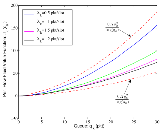
Figure 4: Per-Flow fluid value function $J_{k}\left(q_{k}\right)$ versus queue state $q_{k}$ with $\tau=5$ms, $\gamma_{k}=0.05$ and $L_{kk}=1$ for all $k\in\mathcal{K}$. The two dashed lines represent the functions $\frac{0.2q_{k}^{2}}{\log\left(q_{k}\right)}$ and $\frac{0.7q_{k}^{2}}{\log\left(q_{k}\right)}$.

Corollary 4 suggests that for large queue state $q_{k}$, the per-flow fluid value function increases at the order of $\frac{q_{k}^{2}}{\log\left(q_{k}\right)}$ and is a decreasing function of the average arrival rate $\lambda_{k}$. The analytical result in (49) is also verified in Fig. 4.

IV-B Analysis of Approximation Error

Based on Theorem 2, the approximation error of using the linear architecture $\sum_{k=1}^{K}J_{k}\left(q_{k}\right)$ to approximate $J(\mathbf{q};\mathbf{L})$ is given in the following lemma.

Lemma 7 (Analysis of Approximation Error for Interference Networks).

The approximation error between $J(\mathbf{q};\mathbf{L})$ and $\sum_{k=1}^{K}J_{k}\left(q_{k}\right)$ is given by

$$\big{|}J(\mathbf{q};\mathbf{L})-\sum_{k=1}^{K}J_{k}\left(q_{k}\right)\big{|}=\sum_{k=1}^{K}\sum_{j\neq k}L_{kj}D_{kj}\mathcal{O}\left(\frac{q_{k}q_{j}^{2}+q_{k}^{2}q_{j}}{\log q_{k}\log q_{j}}\right)+\mathcal{O}(L^{2}),\quad\text{as }q_{j},q_{k}\rightarrow\infty,L\rightarrow 0$$ (50)

where the coefficient $D_{kj}$ is given by

$$D_{kj}=\frac{\beta_{k}\beta_{j}}{\gamma_{j}\lambda_{k}\lambda_{j}\tau^{2}}$$ (51)

∎

Proof.

Please refer to Appendix I. ∎

We have the following remark discussing the approximation error in (50).

Remark 5 (Approximation Error w.r.t. System Parameters).

The dependence between the approximation error in (50) and system parameters are given below:

• Approximation Error w.r.t. Traffic Loading: the approximation error is a decreasing function of the average arrival rate $\lambda_{k}$.

• Approximation Error w.r.t. SNR: the approximation error is an increasing function of the SNR per Tx-Rx pair (which is a decreasing function of $\gamma_{k}$).  ∎

IV-C Distributed Power Control Algorithm

As discussed in Section III-C, we can use $\sum_{k=1}^{K}J_{k}\left(q_{k}\right)$ to approximate $V\left(\mathbf{Q}\right)$. Fig. 5 illustrates the quality of the approximation. It can be observed that the sum of the per-flow fluid value functions is a good approximator to the relative value function for both high and low transmit SNR. Using the per-flow fluid value function approximation, i.e.,

$$V\left(\mathbf{Q}\right)\approx\sum_{k=1}^{K}J_{k}\left(q_{k}\right),\quad\forall\mathbf{Q}\in\boldsymbol{\mathcal{Q}}$$ (52)

the distributed power control for the interference network can be obtained by solving the following NUM problem according to Lemma 5.

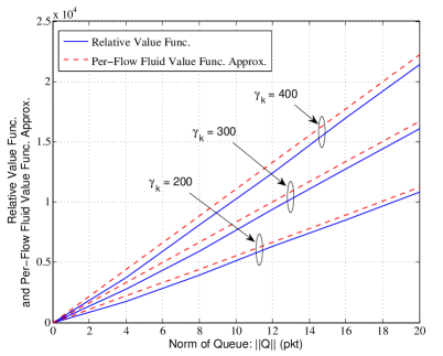
(a) Low Tx SNR regimes with $\gamma_{k}=200$, $\gamma_{k}=300$, $\gamma_{k}=400$, which corresponds to the average Tx SNR per pair being 3.5dB, 3.1dB, 2.9dB (under optimal policy), respectively.

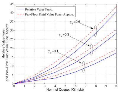
(b) High Tx SNR regimes with $\gamma_{k}=0.1$, $\gamma_{k}=0.3$, $\gamma_{k}=0.6$, which corresponds to the average Tx SNR per pair being 9.7dB, 9.1dB, 8.7dB (under optimal policy), respectively.

Figure 5: Relative value function $V\left(\mathbf{Q}\right)$ and per-flow fluid value function approximation $\sum_{k=1}^{K}J_{k}\left(q_{k}\right)$ versus the norm of the global queue state $\|\mathbf{Q}\|$ with $\mathbf{Q}=\{q_{1},0,\dots,0\}$. The system parameters are configured as in Section IV-D. Note that the relative value functions are calculated using value iteration [4].

Lemma 8 (Equivalent NUM Problem for Interference Networks).

Minimizing the R.H.S. of the Bellman equation in (21) using the per-flow fluid value function approximation in (52) for all $\mathbf{Q}\in\boldsymbol{\mathcal{Q}}$ is equivalent to the following NUM problem:

$$\max_{\boldsymbol{\mathbf{p}}}\ \sum_{k=1}^{K}U_{k}(\mathbf{p}_{k},\boldsymbol{\mathbf{p}}_{-k},\mathbf{L}_{k})$$ (53)

where $\boldsymbol{\mathbf{p}}$, $\mathbf{p}_{k}$, $\boldsymbol{\mathbf{p}}_{-k}$ and $\mathbf{L}_{k}$ are defined in Section II-C. $U_{k}(\mathbf{p}_{k},\boldsymbol{\mathbf{p}}_{-k},\mathbf{L}_{k})$ is the utility function of the $k$-th Tx-Rx pair given by

$$U_{k}(\mathbf{p}_{k},\boldsymbol{\mathbf{p}}_{-k},\mathbf{L}_{k})=\mathbb{E}\left[J_{k}^{\prime}\left(Q_{k}\right)\tau\log\left(1+\frac{p_{k}^{\mathbf{H}}L_{kk}\left|H_{kk}\right|^{2}}{1+\sum_{j\neq k}p_{j}^{\mathbf{H}}L_{kj}\left|H_{kj}\right|^{2}}\right)-\gamma_{k}p_{k}^{\mathbf{H}}\Bigg{|}\mathbf{Q}\right]+\mathcal{O}(\tau^{2}),\text{as }\tau\rightarrow 0$$ (54)

∎

For sufficiently small epoch duration $\tau$, the term $\mathcal{O}(\tau^{2})$ is negligible. Note that the utility function $U_{k}(\mathbf{p}_{k},\boldsymbol{\mathbf{p}}_{-k},\mathbf{L}_{k})$ in (54) is strictly concave in $\mathbf{p}_{k}$ but convex in $\boldsymbol{\mathbf{p}}_{-k}$. Hence, Assumption 6 holds for $U_{k}(\mathbf{p}_{k},\boldsymbol{\mathbf{p}}_{-k},\mathbf{L}_{k})$ in (54) in this example.

Based on Theorem 3, we choose a local objective function $F_{k}(\mathbf{p}_{k},\boldsymbol{\mathbf{p}}_{-k},\mathbf{L}_{k},\mathbf{m}_{-k})$ for the $k$-th sub-system as follows:

$$F_{k}(\mathbf{p}_{k},\boldsymbol{\mathbf{p}}_{-k},\mathbf{L}_{k},\mathbf{m}_{-k})=U_{k}(\mathbf{P}_{k},\boldsymbol{\mathbf{P}}_{-k},\mathbf{L}_{k})-\mathbb{E}\left[p_{k}^{\mathbf{H}}\sum_{j\neq k}m_{j}^{\mathbf{H}}|L_{jk}H_{jk}|^{2}\Bigg{|}\mathbf{Q}\right]$$ (55)

where $\mathbf{m}_{-k}=\{\mathbf{m}_{j}:\forall j\neq k\}$ and $\mathbf{m}_{j}$ is the message of the $j$-th Tx-Rx pair given by

$$\mathbf{m}_{j}=\left\{m_{j}^{\mathbf{H}}=\frac{J_{j}^{\prime}(Q_{j})\tau\Upsilon_{j}^{\mathbf{H}}}{\boldsymbol{\Psi}_{j}^{\mathbf{H}}}:\forall\mathbf{H}\right\}$$ (56)

where $\Upsilon_{j}^{\mathbf{H}}=\frac{p_{j}^{\mathbf{H}}L_{jj}|H_{jj}|^{2}}{1+\sum_{k\neq j}p_{k}^{\mathbf{H}}L_{jk}|H_{jk}|^{2}}$ and $\boldsymbol{\Psi}_{j}^{\mathbf{H}}=1+\sum_{k=1}^{K}p_{k}^{\mathbf{H}}L_{jk}|H_{jk}|^{2}$. Note that $\Upsilon_{j}^{\mathbf{H}}$ and $\boldsymbol{\Psi}_{j}^{\mathbf{H}}$ are the SINR and the total received signal plus noise at receiver $j$ for a given CSI realization $\mathbf{H}$, respectively and both are locally measurable. The associated game for this example is given by

$$(\mathcal{G}1):\quad\max_{\mathbf{p}_{k}}F_{k}(\mathbf{p}_{k},\boldsymbol{\mathbf{p}}_{-k},\mathbf{L}_{k},\mathbf{m}_{-k}),\quad\forall k\in\mathcal{K}$$ (57)

The distributed iterative algorithm solving the game in (57) can be obtained from Algorithm 1 by replacing variable $\mathbf{u}_{k}$ with $\mathbf{p}_{k}$, message $\mathbf{m}_{k}$ in (43) with (56), respectively. Furthermore, according to Corollary 3, as $\mathbf{L}$ goes to zero, the algorithm converges to the unique global optimal point of the NUM problem in (53) for this example.

Define $\boldsymbol{\mathbf{p}}_{-k}^{\mathbf{H}}=\left\{p_{j}^{\mathbf{H}}:\forall j\neq k\right\}$ and $\mathbf{m}_{-k}^{\mathbf{H}}=\left\{m_{j}^{\mathbf{H}}:\forall j\neq k\right\}$ as the collection of coupling effects and messages for a given CSI realization $\mathbf{H}$. Then, the objective function in (57) can be written as

$$F_{k}\left(\mathbf{p}_{k},\boldsymbol{\mathbf{p}}_{-k},\mathbf{L}_{k},\mathbf{m}_{-k}\right)=\mathbb{E}\left[f_{k}\left(p_{k}^{\mathbf{H}},\boldsymbol{\mathbf{p}}_{-k}^{\mathbf{H}},\mathbf{L}_{k},\mathbf{m}_{-k}^{\mathbf{H}}\right)\Big{|}\mathbf{Q}\right]$$ (58)

where $f_{k}\left(p_{k}^{\mathbf{H}},\boldsymbol{\mathbf{p}}_{-k}^{\mathbf{H}},\mathbf{L}_{k},\mathbf{m}_{-k}^{\mathbf{H}}\right)=J_{k}^{\prime}\left(Q_{k}\right)\tau\log\left(1+\frac{p_{k}^{\mathbf{H}}L_{kk}\left|H_{kk}\right|^{2}}{1+\sum_{j\neq k}p_{j}^{\mathbf{H}}L_{kj}\left|H_{kj}\right|^{2}}\right)-p_{k}^{\mathbf{H}}\left(\sum_{j\neq k}m_{j}^{\mathbf{H}}L_{jk}|H_{jk}|^{2}+\gamma_{k}\right)$.

Based on the structure of $F_{k}\left(\mathbf{p}_{k},\boldsymbol{\mathbf{p}}_{-k},\mathbf{L}_{k},\mathbf{m}_{-k}\right)$ in (58), the solution of the game in (57) can be further decomposed into per-CSI control as illustrated in the following Algorithm 2.

Algorithm 2 (Distributed Power Control Algorithm for Interference Networks).

• Step 1 [Information Passing within Each Tx-Rx Pair]: at the beginning of the $t$-th epoch, the $k$-th transmitter notifies the value of $J_{k}^{\prime}\left(Q_{k}\left(t\right)\right)$ to the $k$-th receiver.

• Step 2 [Calculation of Control Actions]: at the beginning of each time slot within the $t$-th epoch with the CSI realization being $\mathbf{H}$, each transmitter determines the transmit power $p_{k}^{\mathbf{H}}$ according to the following per-CSI distributed power allocation algorithm:

  Algorithm 3 (Per-CSI Distributed Power Allocation Algorithm).

  • Step 1 [Initialization]: Set $n=0$. Each transmitter initializes $p_{k}^{\mathbf{H}}(0)$.

  • Step 2 [Message Update and Passing]: Each receiver $k$ locally estimates the SNR $\Upsilon_{m}^{\mathbf{H}}\left(n\right)$ and the total received signal plus noise $\boldsymbol{\Psi}_{k}^{\mathbf{H}}\left(n\right)$. Then, each receiver $k$ calculates $m_{k}^{\mathbf{H}}\left(n\right)$ according to (56) and broadcasts $m_{k}^{\mathbf{H}}\left(n\right)$ to all the transmitters.

  • Step 3 [Power Action Update]: After receiving messages $\{m_{k}^{\mathbf{H}}\left(n\right)\}$ from all the receivers, each transmitter locally updates $p_{k}^{\mathbf{H}}\left(n+1\right)$ according to

    $$\ p_{k}^{\mathbf{H}}\left(n+1\right) =\arg\max_{p_{k}^{\mathbf{H}}}f_{k}\left(p_{k}^{\mathbf{H}},\boldsymbol{\mathbf{p}}_{-k}^{\mathbf{H}}\left(n\right),\mathbf{L}_{k},\mathbf{m}_{-k}^{\mathbf{H}}\left(n\right)\right)$$

    $$=\min\left\{\left(\frac{J_{k}^{\prime}\left(Q_{k}\left(t\right)\right)\tau}{\sum_{j\neq k}m_{j}^{\mathbf{H}}\left(n\right)L_{jk}|H_{jk}\left(n\right)|^{2}+\gamma_{k}}-\frac{1+I_{k}\left(n\right)}{L_{kk}|H_{kk}\left(n\right)|^{2}}\right)^{+},\ p_{k}^{up}\left(t_{n}\right)\right\}$$ (59)

    where $I_{k}\left(n\right)=\sum_{j\neq k}p_{j}^{\mathbf{H}}\left(n\right)L_{kj}|H_{kj}\left(n\right)|^{2}$ is the total interference at receiver $k$. $p_{k}^{up}\left(t_{n}\right)$ satisfies $\log\left(1+\frac{p_{k}^{up}\left(t_{n}\right)L_{kk}|H_{kk}\left(n\right)|^{2}}{1+I_{k}\left(n\right)}\right)\tau^{\prime}=Q\left(t_{n}\right)$, where $\tau^{\prime}$ is the slot duration and $Q\left(t_{n}\right)$ is the QSI at the $n$-th time slot of the $t$-th epoch.

  • Step 4 [Termination]: If a certain termination condition is satisfied, stop. Otherwise, $n=n+1$ and go to Step 2 of Algorithm 3.  ∎

Fig. 6 illustrates the above procedure in a flow chart.

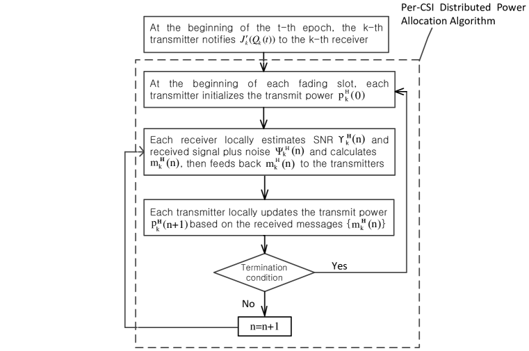
Figure 6: Algorithm flow of the proposed distributive power control algorithm for the interference networks.

Remark 6 (Multi-level Water-filling Structure of the Power Action Update).

The power action update in (59) in Algorithm 3 has the multi-level water-filling structure where the power is allocated according to the CSI but the water-level is adaptive to the QSI indirectly via the per-flow fluid value function $J_{k}\left(Q_{k}\right)$.  ∎

IV-D Simulation Results and Discussions

In this subsection, we compare the delay performance gain of the proposed distributed power control scheme in Algorithm 2 for the interference networks example with the following three baseline schemes using numerical simulations.

• Baseline 1 [Orthogonal Transmission]: The transmissions among the $K$ Tx-Rx pairs are coordinated using TDMA. At each time slot, the Tx-Rx pair with the largest channel gain is select to transmit and the resulting power allocation is adaptive to the CSI only.

• Baseline 2 [CSI Only Scheme]: CSI Only scheme solves the problem with the objective function given in (54) replacing $J_{k}^{\prime}\left(Q_{k}\right)$ with constant 1. The corresponding power control algorithm can be obtained by replacing $J_{k}^{\prime}\left(Q_{k}\right)$ with constant 1 in Algorithm 2 and the resulting power allocation is adaptive to the CSI only.

• Baseline 3 [Queue-Weighted Throughput-Optimal (QWTO) Scheme]: QWTO scheme solves the problem with the objective function given in (54) replacing $J_{k}^{\prime}\left(Q_{k}\right)$ with $Q_{k}$. The corresponding power control algorithm can be obtained by replacing $J_{k}^{\prime}\left(Q_{k}\right)$ with $Q_{k}$ in Algorithm 2 and the resulting power allocation is adaptive to the CSI and the QSI.

In the simulations, we consider a symmetric system with $K$ Tx-Rx pairs in the fast fading environment, where the microscopic fading coefficient and the channel noise are $\mathcal{CN}\left(0,1\right)$ distributed. The direct channel long term path gain is $L_{kk}=1$ for all $k\in\mathcal{K}$ and the cross-channel path gain is $L_{kj}=0.1$ for all $k,j\in\mathcal{K},k\neq j$ as in [28]. We consider Poisson packet arrival with average arrival rate $\lambda_{k}$ (pkts/epoch). The packet size is exponentially distributed with mean size equal to $30$K bits. The decision epoch duration $\tau$ is $5$ms. The total bandwidth is $10$MHz. Furthermore, $\gamma_{k}$ is the same and $\beta_{k}=1$ for all $k\in\mathcal{K}$.

Fig. 7 illustrates the average delay per pair versus the average transmit SNR. The average delay of all the schemes decreases as the average transmit SNR increases. It can be observed that there is significant performance gain of the proposed scheme compared with all the baselines. It also verifies that the sum of the per-flow fluid value functions is a good approximator to the relative value function.

Fig. 8 illustrates the average delay per pair versus the traffic loading (average data arrival rate $\lambda_{k}$). The proposed scheme achieves significant performance gain over all the baselines across a wide range of the input traffic loading. In addition, as $\lambda_{k}$ increases, the performance gain of the proposed scheme also increases compared with all the baselines. This verifies Theorem 1 and Lemma 7. Specifically, it is because as the traffic loading increases, the chance for the queue state at large values increases, which means that $J\left(\mathbf{q};\mathbf{L}\right)$ becomes a good approximator for $V\left(\mathbf{Q}\right)$ according to Remark 1. Furthermore, the approximation error between $J\left(\mathbf{q};\mathbf{L}\right)$ and $\sum_{k=1}^{K}J\left(q_{k}\right)$ also decreases according to Remark 5. Therefore, the per-flow fluid value function approximation in (52) becomes more accurate as $\lambda_{k}$ increases.

Fig. 9 illustrates the average delay per pair versus the number of the Tx-Rx pairs. The average delay of all the schemes increases as the number of the Tx-Rx pairs increases. This is due to the increasing of the total interference for each Tx-Rx pair. It can be observed that there is significant performance gain of the proposed scheme compared with all the baselines across a wide range of the number of the Tx-Rx pairs.

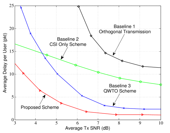
Figure 7: Average delay per pair versus average transmit SNR. The number of the Tx-Rx pair is $K=5$ and the average data arrival rate is $\lambda_{k}=1$ pkt/epoch for all $k\in\mathcal{K}$.

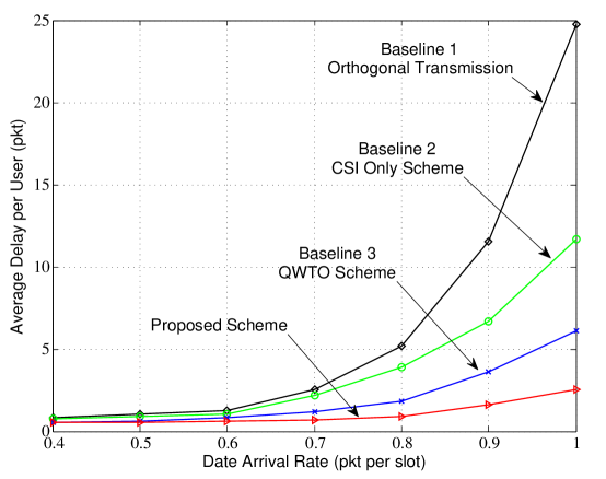
Figure 8: Average delay per pair versus average data arrival rate at average transmit SNR $6$ dB. The number of the Tx-Rx pair is $K=5$.

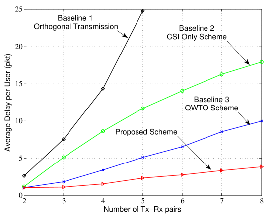
Figure 9: Average delay per pair versus number of Tx-Rx pairs at average transmit SNR $6$ dB. The average data arrival rate is $\lambda_{k}=1$ pkt/epoch for all $k\in\mathcal{K}$.

V Summary

In this paper, we propose a framework of solving the infinite horizon average cost problem for the weakly coupled multi-dimensional systems. To reduce the computational complexity, we first introduce the VCTS and obtain the associated fluid value function to approximate the relative value function of the ODTS. To further address the low complexity distributed solution requirement and the coupling challenge, we model the weakly coupled system as a perturbation of a decoupled base system. We then use the sum of the per-flow fluid value functions, which are obtained by solving the per-flow HJB equations under each sub-system, to approximate the fluid value function of the VCTS. Finally, using per-flow fluid value function approximation, we obtain the distributed solution by solving an equivalent deterministic NUM problem. Moreover, we also elaborate on how to use this framework in the interference networks example. It is shown by simulations that the proposed distributed power control algorithm has much better delay performance than the other three baseline schemes.

Appendix A: Proof of Corollary 1

We first write the state dynamics in (1) in the following form:

$$\mathbf{x}_{k}(t+1)=\mathbf{x}_{k}\left(t\right)+\left(\mathbf{f}_{k}\left(\mathbf{u}_{k}\left(t\right),\mathbf{u}_{-k}\left(t\right),\boldsymbol{\epsilon}_{k}\right)+\mathbf{z}_{k}\left(t\right)\right)\Delta$$

Assume $V\left(\mathbf{x}\right)$ is of class $\mathcal{C}^{1}$, we have the following Taylor expansion on $V\left(\mathbf{x}(t+1)\right)$ in (7):

$$\mathbb{E}\left[V\left(\mathbf{x}(t+1)\right)\big{|}\mathbf{x}\left(t\right)=\mathbf{x},\Omega\left(\mathbf{x}\right)\right]=V\left(\mathbf{x}\right)+\nabla_{\mathbf{x}}V\left(\mathbf{x}\right)\left[\mathbf{f}\left(\Omega\left(\mathbf{x}\right),\boldsymbol{\epsilon}\right)+\overline{\mathbf{z}}\right]^{T}\Delta+\mathcal{O}\left(\Delta^{2}\right)$$

Hence, the Bellman equation in (7) becomes:

$$\theta^{\ast}\Delta=\min_{\Omega\left(\mathbf{x}\right)}\left[c\left(\mathbf{x},\Omega\left(\mathbf{x}\right)\right)\Delta+\nabla_{\mathbf{x}}V\left(\mathbf{x}\right)\left[\mathbf{f}\left(\Omega\left(\mathbf{x}\right),\boldsymbol{\epsilon}\right)+\overline{\mathbf{z}}\right]^{T}\Delta+\mathcal{O}\left(\Delta^{2}\right)\right]$$

Suppose $\left(\theta^{\ast},V^{\ast},\mathbf{u}^{\ast}\right)$ satisfies the Bellman equation in (7), we have

$$-\theta^{\ast}+c\left(\mathbf{x},\mathbf{u}^{\ast}\right)+\nabla_{\mathbf{x}}V^{\ast}\left(\mathbf{x}\right)\left[\mathbf{f}\left(\mathbf{u}^{\ast},\boldsymbol{\epsilon}\right)+\overline{\mathbf{z}}\right]^{T}+\mathcal{O}\left(\Delta\right) =0,\quad\forall\mathbf{x}\in\boldsymbol{\mathcal{X}}$$ (60)

$$\nabla_{\mathbf{u}_{k}}c_{k}\left(\mathbf{x}_{k},\mathbf{u}_{k}^{\ast}\right)+\nabla_{\mathbf{x}}V^{\ast}\left(\mathbf{x}\right)\left[\nabla_{\mathbf{u}_{k}}\mathbf{f}\left(\mathbf{u}^{\ast},\boldsymbol{\epsilon}\right)+\overline{\mathbf{z}}\right]^{T}+\mathcal{O}\left(\Delta\right) =\mathbf{0},\quad\forall k\in\mathcal{K}$$ (61)

where $\nabla_{\mathbf{u}_{k}}\mathbf{f}\left(\mathbf{u},\boldsymbol{\epsilon}\right)=\left(\nabla_{\mathbf{u}_{k}}\mathbf{f}_{1}\left(\mathbf{u}_{1},\mathbf{u}_{-1},\boldsymbol{\epsilon}_{1}\right),\dots,\nabla_{\mathbf{u}_{k}}\mathbf{f}_{K}\left(\mathbf{u}_{K},\mathbf{u}_{-K},\boldsymbol{\epsilon}_{K}\right)\right)$. (60) and (61) can be expressed as a fixed point equation in $\left(\theta^{\ast},V^{\ast},\mathbf{u}^{\ast}\right)$:

$$\mathbf{F}\left(\theta^{\ast},V^{\ast},\mathbf{u}^{\ast}\right)=\mathbf{0}$$ (62)

Suppose $\big{(}\tilde{\theta}^{\ast},V,\mathbf{u}\big{)}$ is the solution of the approximate Bellman equation in (9), we have

$$-\tilde{\theta}^{\ast}+c\left(\mathbf{x},\mathbf{u}\right)+\nabla_{\mathbf{x}}V\left(\mathbf{x}\right)\left[\mathbf{f}\left(\mathbf{u},\boldsymbol{\epsilon}\right)+\overline{\mathbf{z}}\right]^{T}=0,\quad\forall\mathbf{x}\in\boldsymbol{\mathcal{X}}$$ (63)

$$\nabla_{\mathbf{u}_{k}}c_{k}\left(\mathbf{x}_{k},\mathbf{u}_{k}\right)+\nabla_{\mathbf{x}}V\left(\mathbf{x}\right)\left[\nabla_{\mathbf{u}_{k}}\mathbf{f}\left(\mathbf{u},\boldsymbol{\epsilon}\right)+\overline{\mathbf{z}}\right]^{T}=0,\quad\forall k\in\mathcal{K}$$ (64)

Comparing (63) and (64) with (60) and (61), $\big{(}\tilde{\theta}^{\ast},V,\mathbf{u}\big{)}$ can be visualized as a solution of the perturbed fixed point equation:

$$\mathbf{F}\big{(}\tilde{\theta}^{\ast},V,\mathbf{u}\big{)}=\mathcal{O}(\Delta)$$ (65)

Hence, we have $\theta^{\ast}=\tilde{\theta}^{\ast}+\delta_{\theta}$, $V^{\ast}(\mathbf{Q})=V(\mathbf{Q})+\delta_{V}$ and $\mathbf{u}^{\ast}=\mathbf{u}+\boldsymbol{\delta}_{\mathbf{u}}$ and $(\delta_{\theta},\delta_{V},\boldsymbol{\delta}_{\mathbf{u}})$ satisfies

$$\mathrm{d}\mathbf{F}\left(\theta^{\ast},V^{\ast},\mathbf{u}^{\ast}\right)=\frac{\partial\mathbf{F}\left(\theta^{\ast},V^{\ast},\mathbf{u}^{\ast}\right)}{\partial\theta}\delta_{\theta}+\frac{\partial\mathbf{F}\left(\theta^{\ast},V^{\ast},\mathbf{u}^{\ast}\right)}{\partial V}\delta_{V}+\nabla_{\mathbf{u}}\mathbf{F}\left(\theta^{\ast},V^{\ast},\mathbf{u}^{\ast}\right)\boldsymbol{\delta}_{\mathbf{u}}$$ (66)

Comparing (65) with (63), we have $\mathrm{d}\mathbf{F}\left(\theta^{\ast},V^{\ast},\mathbf{u}^{\ast}\right)=\mathcal{O}(\Delta)$. Hence, we have

$$\frac{\partial\mathbf{F}\left(\theta^{\ast},V^{\ast},\mathbf{u}^{\ast}\right)}{\partial\theta}\delta_{\theta}+\frac{\partial\mathbf{F}\left(\theta^{\ast},V^{\ast},\mathbf{u}^{\ast}\right)}{\partial V}\delta_{V}+\nabla_{\mathbf{u}}\mathbf{F}\left(\theta^{\ast},V^{\ast},\mathbf{u}^{\ast}\right)\boldsymbol{\delta}_{\mathbf{u}}=\mathcal{O}(\Delta)$$

Therefore, $(\delta_{\theta},\delta_{V},\boldsymbol{\delta}_{\mathbf{u}})=\mathcal{O}(\Delta)$.

Appendix B: Proof of Corollary 2

First, It can be observed that if ($c^{\infty},\{J\left(\mathbf{x}\right)\}$) satisfies the HJB equation in (26), then it also satisfies the approximate HJB equation in (9). Second, if $J\left(\mathbf{x}\right)=\mathcal{O}\left(|\mathbf{x}|^{n}\right)$ is polynomial growth at order $n$, we have $\mathbb{E}^{\Omega^{v}}\left[J\left(\mathbf{x}\right)\right]<\infty$ for any admissible policy $\Omega^{v}$. Hence, $J\left(\mathbf{x}\right)$ satisfies the transversality condition of the approximate Bellman equation. Therefore, we have $\theta^{\ast}=\tilde{\theta}^{\ast}+\mathcal{O}\left(\Delta\right)=c^{\infty}+\mathcal{O}\left(\Delta\right)$.

Appendix A: Proof of Theorem 1

In the following proof, we first establish three important equalities in (67), (Appendix A: Proof of Theorem 1) and (Appendix A: Proof of Theorem 1). We then prove Theorem 1 based on the three equalities.

First, we establish the following equality:

$$\frac{1}{n^{2}}\mathbb{E}\left[V\left(\mathbf{x}^{\ast}\left(\lfloor nT\rfloor;n\mathbf{x}^{n}\right)\right)\right]=\frac{1}{n^{2}}\Big{[}V\left(n\mathbf{x}^{n}\right)-\sum_{i=0}^{\lfloor nT\rfloor-1}\mathbb{E}\left[\widetilde{c}\left(\mathbf{x}^{\ast}\left(i;n\mathbf{x}^{n}\right),\mathbf{u}^{\ast}\left(\mathbf{x}^{\ast}\left(i;n\mathbf{x}^{n}\right)\right)\right)\right]\Big{]}+\mathcal{O}\left(\frac{1}{n}\right)$$ (67)

Here we define $\mathbf{x}\left(t;\mathbf{x}_{0}\right)$ and $\overline{\mathbf{x}}(t;\mathbf{x}_{0})$ to be the system states at time $t$ which evolve according to the dynamics in (1) and (23), respectively with initial state $\mathbf{x}_{0}$. Let $N$ be the dimension of $\mathbf{x}$ and let $\mathbf{u}^{\ast}$ be the optimal policy solving Problem 1. Then, we write the Bellman equation in (7) in a vector form as: $\theta\mathbf{e}+\mathbf{V}=\mathbf{c}\left(\mathbf{u}^{\ast}\right)+\mathbf{P}\left(\mathbf{u}^{\ast}\right)\mathbf{V}$ where $\mathbf{e}$ is a $N\times 1$ vector with each element being $1$, $\mathbf{P}\left(\mathbf{u}^{\ast}\right)$ is a $N\times N$ transition matrix, $\mathbf{c}\left(\mathbf{u}^{\ast}\right)$ and $\mathbf{V}$ are $N\times 1$ cost and value function vectors. We iterate the vector form Bellman equation as follows:

$$\mathbf{P}\left(\mathbf{u}^{\ast}\right)\mathbf{V} =\mathbf{V}-\left(\mathbf{c}\left(\mathbf{u}^{\ast}\right)-\theta\mathbf{e}\right)$$

$$\mathbf{P}^{2}\left(\mathbf{u}^{\ast}\right)\mathbf{V} =\mathbf{P}\left(\mathbf{u}^{\ast}\right)\mathbf{V}-\mathbf{P}\left(\mathbf{u}^{\ast}\right)\left(\mathbf{c}\left(\mathbf{u}^{\ast}\right)-\theta\mathbf{e}\right)$$

$$=\mathbf{V}-\left(\mathbf{c}\left(\mathbf{u}^{\ast}\right)-\theta\mathbf{e}\right)-\mathbf{P}\left(\mathbf{u}^{\ast}\right)\left(\mathbf{c}\left(\mathbf{u}^{\ast}\right)-\theta\mathbf{e}\right)$$

$$\vdots$$

$$\mathbf{P}^{m}\left(\mathbf{u}^{\ast}\right)\mathbf{V} =\mathbf{V}-\sum_{i=0}^{m-1}\mathbf{P}^{i}\left(\mathbf{u}^{\ast}\right)\left(\mathbf{c}\left(\mathbf{u}^{\ast}\right)-\theta\mathbf{e}\right)$$ (68)

Considering the row corresponding to a given system state $\mathbf{x}_{0}$, we have

$$\mathbb{E}\left[V\left(\mathbf{x}^{\ast}\left(m;\mathbf{x}_{0}\right)\right)\right]=V\left(\mathbf{x}_{0}\right)-\sum_{i=0}^{m-1}\left(\mathbb{E}\left[c\left(\mathbf{x}^{\ast}\left(i;\mathbf{x}_{0}\right),\mathbf{u}^{\ast}\left(\mathbf{x}^{\ast}\left(i;\mathbf{x}_{0}\right)\right)\right)\right]-\theta\right)$$ (69)

where $\mathbf{x}^{\ast}\left(t;\mathbf{x}_{0}\right)$ is the system state under optimal policy $\mathbf{u}^{\ast}$ with initial state $\mathbf{x}_{0}$. Dividing $n^{2}$ on both size of (69), choosing $m=\lfloor nT\rfloor$ and $\mathbf{x}_{0}=n\mathbf{x}^{n}$, we have

$$\frac{1}{n^{2}}\mathbb{E}\left[V\left(\mathbf{x}^{\ast}\left(\lfloor nT\rfloor;n\mathbf{x}^{n}\right)\right)\right]=\frac{1}{n^{2}}\Big{[}V\left(n\mathbf{x}^{n}\right)-\sum_{i=0}^{\lfloor nT\rfloor-1}\mathbb{E}\left[c\left(\mathbf{x}^{\ast}\left(i;n\mathbf{x}^{n}\right),\mathbf{u}^{\ast}\left(\mathbf{x}^{\ast}\left(i;n\mathbf{x}^{n}\right)\right)\right)\right]\Big{]}+\mathcal{O}\left(\frac{1}{n}\right)$$

$$=\frac{1}{n^{2}}\Big{[}V\left(n\mathbf{x}^{n}\right)-\sum_{i=0}^{\lfloor nT\rfloor-1}\mathbb{E}\left[\widetilde{c}\left(\mathbf{x}^{\ast}\left(i;n\mathbf{x}^{n}\right),\mathbf{u}^{\ast}\left(\mathbf{x}^{\ast}\left(i;n\mathbf{x}^{n}\right)\right)\right)\right]\Big{]}+\mathcal{O}\left(\frac{1}{n}\right)$$ (70)

where the first equality is due to $\frac{1}{n^{2}}\sum_{i=0}^{\lfloor nT\rfloor-1}\theta=\mathcal{O}\left(\frac{1}{n}\right)$ last equality is due to $\widetilde{c}\left(\overline{\mathbf{x}},\mathbf{u}\right)=c\left(\overline{\mathbf{x}},\mathbf{u}\right)-c^{\infty}$ and $\frac{1}{n^{2}}\sum_{i=0}^{\lfloor nT\rfloor-1}c^{\infty}=\left(\frac{1}{n}\right)$.

Second, we establish the following equality which holds under any unichain stationary policy $\mathbf{u}$:

$$\frac{1}{n^{2}}\sum_{i=0}^{nT^{n}}\widetilde{c}\left(\mathbf{x}\left(i;n\mathbf{x}^{n}\right),\mathbf{u}\left(\mathbf{x}\left(i;n\mathbf{x}^{n}\right)\right)\right)$$

$$= \int_{0}^{T^{n}}\widetilde{c}\left(\overline{\mathbf{x}}^{n}\left(t;\mathbf{x}^{n}\right),\mathbf{u}\left(\overline{\mathbf{x}}^{n}\left(t;\mathbf{x}^{n}\right)\right)\right)\mathrm{d}t-\int_{0}^{T^{n}}\sum_{k=1}^{K}\widetilde{g}_{k}\left(\mathbf{u}_{k}\left(\overline{\mathbf{x}}^{n}\left(t;\mathbf{x}^{n}\right)\right)\right)\mathrm{d}t+\mathcal{O}\left(\frac{1}{n}\right)$$ (71)

where $T^{n}=\frac{1}{n}\lfloor nT\rfloor$. Here we define a scaled process w.r.t. $\mathbf{x}\left(t\right)$ as

$$\overline{\mathbf{x}}^{n}(t;\mathbf{x}_{0}^{n})=\frac{1}{n}\mathbf{x}(nt;n\mathbf{x}_{0}^{n}),\quad\text{where \ }\mathbf{x}_{0}^{n}=\frac{1}{n}\lfloor n\mathbf{x}_{0}\rfloor$$ (72)

$\lfloor\mathbf{x}\rfloor$ is the floor function that maps each element of $\mathbf{x}$ to the integer not greater than it. According to Prop.3.2.3 of [1], we have $\lim_{n\rightarrow\infty}\overline{\mathbf{x}}^{n}(t;\mathbf{x}_{0}^{n})=\overline{\mathbf{x}}^{vt}(t;\mathbf{x}_{0})$, where $\overline{\mathbf{x}}^{vt}$ is some fluid process w.r.t. $\mathbf{x}$. In the fluid control problem in Problem 3, for each initial state $\mathbf{x}_{0}\in\boldsymbol{\mathcal{X}}$, there is a finite time horizon $T$ such that $\overline{\mathbf{x}}^{vt}(t;\mathbf{x}_{0})=\mathbf{0}$ for all $t\geq T$ [10]. Furthermore, we can write the above convergence result based on the functional law of large numbers as $\overline{\mathbf{x}}^{n}(t;\mathbf{x}_{0}^{n})=\overline{\mathbf{x}}^{vt}(t;\mathbf{x}_{0})+\mathcal{O}\left(\sqrt{\frac{\log\log n}{n}}\right)$. Before proving (Appendix A: Proof of Theorem 1), we show the following lemma.

Lemma 9.

For the continuously differentiable function $g_{k}$ in the cost function in (4) with $\left|g_{k}\left(\mathbf{u}_{k}\right)\right|<\infty$ $\left(\forall\mathbf{u}_{k}\in\mathcal{U}_{k}\right)$, there exist a finite constant $C$, such that for all $k$, $t$, we have

$$\left|\int_{t}^{t+1}\widetilde{g}_{k}\left(\mathbf{u}_{k}\left(\widetilde{\mathbf{x}}\left(t;\mathbf{x}_{0}\right)\right)\right)\mathrm{d}s-\frac{1}{2}\left[\widetilde{g}_{k}\left(\mathbf{u}_{k}\left(\mathbf{x}\left(t;\mathbf{x}_{0}\right)\right)\right)+\widetilde{g}_{k}\left(\mathbf{u}_{k}\left(\mathbf{x}\left(t+1;\mathbf{x}_{0}\right)\right)\right)\right]\right|\leq C,\quad\forall\mathbf{x}_{0}\in\boldsymbol{\mathcal{X}}$$ (73)

where $\widetilde{g}_{k}\left(\mathbf{u}_{k}\right)\triangleq g_{k}\left(\mathbf{u}_{k}\right)-\frac{c^{\infty}}{K}$, $\widetilde{\mathbf{x}}\left(t;\mathbf{x}_{0}\right)$ is a piecewise linear function and satisfies $\widetilde{\mathbf{x}}\left(t;\mathbf{x}_{0}\right)=\mathbf{x}\left(t;\mathbf{x}_{0}\right)$ for all $t\in\mathbb{Z}^{\ast}$. Furthermore, for a given finite positive real number $\kappa$, we have

$$\left|\widetilde{g}_{k}\left(\mathbf{u}_{k}\left(\kappa\mathbf{x}_{0}\right)\right)-\kappa\widetilde{g}_{k}\left(\mathbf{u}_{k}\left(\mathbf{x}_{0}\right)\right)\right|=\mathcal{O}\left(\kappa\right),\quad\forall\mathbf{x}_{0}\in\boldsymbol{\mathcal{X}}$$ (74)

∎

Since $\mathbf{u}_{k}\in\mathcal{U}_{k}$ and $\left|\widetilde{g}_{k}\left(\mathbf{u}_{k}\right)\right|<\infty$ $\left(\forall\mathbf{u}_{k}\in\mathcal{U}_{k}\right)$, the two inequalities in (73) and (74) can be easily verified using the compactness property of the sub-system action space $\mathcal{U}_{k}$. We establish the proof of (Appendix A: Proof of Theorem 1) in the following two steps.

1. First, we prove the following equality:

   $$\frac{1}{n^{2}}\int_{0}^{nT^{n}}\widetilde{c}\left(\widetilde{\mathbf{x}}\left(t;n\mathbf{x}^{n}\right),\mathbf{u}\left(\widetilde{\mathbf{x}}\left(t;n\mathbf{x}^{n}\right)\right)\right)\mathrm{d}t=\frac{1}{n^{2}}\sum_{i=0}^{nT^{n}}\widetilde{c}\left(\mathbf{x}\left(i;n\mathbf{x}^{n}\right),\mathbf{u}\left(\mathbf{x}\left(i;n\mathbf{x}^{n}\right)\right)\right)+\mathcal{O}\left(\frac{1}{n}\right)$$ (75)

   We calculate $\int_{0}^{nT^{n}}\widetilde{c}\left(\widetilde{\mathbf{x}}\left(t;n\mathbf{x}^{n}\right),\mathbf{u}\left(\widetilde{\mathbf{x}}\left(t;n\mathbf{x}^{n}\right)\right)\right)\mathrm{d}t$ and $\sum_{i=0}^{nT^{n}}\widetilde{c}\left(\mathbf{x}\left(i;n\mathbf{x}^{n}\right),\mathbf{u}\left(\mathbf{x}\left(i;n\mathbf{x}^{n}\right)\right)\right)$ in (75) as follows

   $$\int_{0}^{nT^{n}}\widetilde{c}\left(\widetilde{\mathbf{x}}\left(t;n\mathbf{x}^{n}\right),\mathbf{u}\left(\widetilde{\mathbf{x}}\left(t;n\mathbf{x}^{n}\right)\right)\right)\mathrm{d}t$$

   $$= \sum_{i=0}^{nT^{n}-1}\sum_{k=1}^{K}\frac{1}{2}\left[\alpha_{k}\|\mathbf{x}_{k}(t;n\mathbf{x}^{n})\|_{\mathbf{v}_{k},1}+\alpha_{k}\|\mathbf{x}_{k}(t+1;n\mathbf{x}^{n})\|_{\mathbf{v}_{k},1}\right]+\int_{0}^{nT^{n}}\sum_{k=1}^{K}\widetilde{g}_{k}\left(\mathbf{u}_{k}\left(\widetilde{\mathbf{x}}\left(t;n\mathbf{x}^{n}\right)\right)\right)\mathrm{d}t$$ (76)

   $$\sum_{i=0}^{nT^{n}}\widetilde{c}\left(\mathbf{x}\left(i;n\mathbf{x}^{n}\right),\mathbf{u}\left(\mathbf{x}\left(i;n\mathbf{x}^{n}\right)\right)\right)$$

   $$= \sum_{i=0}^{nT^{n}-1}\sum_{k=1}^{K}\frac{1}{2}\left[\alpha_{k}\|\mathbf{x}_{k}(t;n\mathbf{x}^{n})\|_{\mathbf{v}_{k},1}+\alpha_{k}\|\mathbf{x}_{k}(t+1;n\mathbf{x}^{n})\|_{\mathbf{v}_{k},1}\right.$$

   $$\hskip 113.81102pt\left.+\widetilde{g}_{k}\left(\mathbf{u}_{k}\left(\mathbf{x}\left(t;n\mathbf{x}^{n}\right)\right)\right)+\widetilde{g}_{k}\left(\mathbf{u}_{k}\left(\mathbf{x}\left(t+1;n\mathbf{x}^{n}\right)\right)\right)\right]+n^{2}\mathcal{E}^{n}$$ (77)

   where we denote $\mathcal{E}^{n}=\frac{1}{2n^{2}}\left[\widetilde{c}\left(\mathbf{x}\left(0;n\mathbf{x}^{n}\right),\mathbf{u}\left(\mathbf{x}\left(0;n\mathbf{x}^{n}\right)\right)\right)+\widetilde{c}\left(\mathbf{x}\left(nT^{n};n\mathbf{x}^{n}\right),\mathbf{u}\left(\mathbf{x}\left(nT^{n};n\mathbf{x}^{n}\right)\right)\right)\right]$. Then based on (76) and (77), we have

   $$\frac{\left|(\ref{impp111})-(\ref{impp222})\right|}{n^{2}}=\left|\frac{1}{n^{2}}\int_{0}^{nT^{n}}\widetilde{c}\left(\widetilde{\mathbf{x}}\left(t;n\mathbf{x}^{n}\right),\mathbf{u}\left(\widetilde{\mathbf{x}}\left(t;n\mathbf{x}^{n}\right)\right)\right)\mathrm{d}t-\frac{1}{n^{2}}\sum_{i=0}^{nT^{n}}\widetilde{c}\left(\mathbf{x}\left(i;n\mathbf{x}^{n}\right),\mathbf{u}\left(\mathbf{x}\left(i;n\mathbf{x}^{n}\right)\right)\right)\right|$$

   $$= \frac{1}{n^{2}}\left|\int_{0}^{nT^{n}}\sum_{k=1}^{K}\widetilde{g}_{k}\left(\mathbf{u}_{k}\left(\widetilde{\mathbf{x}}\left(t;n\mathbf{x}^{n}\right)\right)\right)\right.\left.-\sum_{i=0}^{nT^{n}-1}\sum_{k=1}^{K}\frac{1}{2}\left[\widetilde{g}_{k}\left(\mathbf{u}_{k}\left(\mathbf{x}\left(t;n\mathbf{x}^{n}\right)\right)\right)+\widetilde{g}_{k}\left(\mathbf{u}_{k}\left(\mathbf{x}\left(t+1;n\mathbf{x}^{n}\right)\right)\right)\right]+n^{2}\mathcal{E}^{n}\right|$$

   $$\overset{(a)}{=} \mathcal{O}\left(\frac{1}{n}\right)+\left|\mathcal{E}^{n}\right|$$ (78)

   where $(a)$ is due to the triangle inequality and (73). Next, we prove $\mathcal{E}^{n}=\mathcal{O}\left(\frac{1}{n}\right)$ as follows

   $$\mathcal{E}^{n}=\frac{1}{2n^{2}}\sum_{k=1}^{K}\left[\left(\alpha_{k}\|\mathbf{x}_{k}\left(0;n\mathbf{x}^{n}\right)\|_{\mathbf{v}_{k},1}+\widetilde{g}_{k}\left(\mathbf{u}_{k}\left(\mathbf{x}\left(0;n\mathbf{x}^{n}\right)\right)\right)\right)\right.$$

   $$\left.+\left(\alpha_{k}\|\mathbf{x}_{k}\left(nT^{n};n\mathbf{x}^{n}\right)\|_{\mathbf{v}_{k},1}+\widetilde{g}_{k}\left(\mathbf{u}_{k}\left(\mathbf{x}\left(nT^{n};n\mathbf{x}^{n}\right)\right)\right)\right)\right]\overset{(b)}{=}\frac{\mathcal{O}\left(n\right)}{2n^{2}}=\mathcal{O}\left(\frac{1}{n}\right)$$ (79)

   where $(b)$ is due to $\|\mathbf{x}_{k}\left(0;n\mathbf{x}^{n}\right)\|_{\mathbf{v}_{k},1}=\|n\mathbf{x}_{k}^{n}\|_{\mathbf{v}_{k},1}=\mathcal{O}\left(n\right)$, $\|\mathbf{x}_{k}\left(nT^{n};n\mathbf{x}^{n}\right)\|_{\mathbf{v}_{k},1}=\|n\mathbf{x}_{k}^{n}+\sum_{i=1}^{nT^{n}-1}\left(\mathbf{f}_{k}\left(\mathbf{u}_{k}(i),\mathbf{u}_{-k}(i),\boldsymbol{\epsilon}\right)+\mathbf{z}_{k}(i)\right)\|_{\mathbf{v}_{k},1}=\mathcal{O}\left(n\right)$, and $\\ \lim_{n\rightarrow\infty}\frac{1}{2n^{2}}\left[g_{k}\left(\mathbf{u}_{k}\left(\mathbf{x}\left(0;n\mathbf{x}^{n}\right)\right)\right)\right.\left.+g_{k}\left(\mathbf{u}_{k}\left(\mathbf{x}\left(nT^{n};n\mathbf{x}^{n}\right)\right)\right)\right]=0$.

   Combining (78) and (79), we have (75).

2. Second, we prove the following equality:

   $$\frac{1}{n^{2}}\int_{0}^{nT^{n}}\widetilde{c}\left(\widetilde{\mathbf{x}}\left(t;n\mathbf{x}^{n}\right),\mathbf{u}\left(\widetilde{\mathbf{x}}\left(t;n\mathbf{x}^{n}\right)\right)\right)\mathrm{d}t$$

   $$= \int_{0}^{T^{n}}\widetilde{c}\left(\overline{\mathbf{x}}^{n}\left(t;\mathbf{x}^{n}\right),\mathbf{u}\left(\overline{\mathbf{x}}^{n}\left(t;\mathbf{x}^{n}\right)\right)\right)\mathrm{d}t-\int_{0}^{T^{n}}\sum_{k=1}^{K}\widetilde{g}_{k}\left(\mathbf{u}_{k}\left(\overline{\mathbf{x}}^{n}\left(t;\mathbf{x}^{n}\right)\right)\right)\mathrm{d}t+\mathcal{O}\left(\frac{1}{n}\right)$$ (80)

   We have

   $$\frac{1}{n^{2}}\int_{0}^{nT^{n}}\widetilde{c}\left(\widetilde{\mathbf{x}}\left(t;n\mathbf{x}^{n}\right),\mathbf{u}\left(\widetilde{\mathbf{x}}\left(t;n\mathbf{x}^{n}\right)\right)\right)\mathrm{d}t\overset{(d)}{=}\frac{1}{n}\int_{0}^{T^{n}}\widetilde{c}\left(\widetilde{\mathbf{x}}\left(nt;n\mathbf{x}^{n}\right),\mathbf{u}\left(\widetilde{\mathbf{x}}\left(nt;n\mathbf{x}^{n}\right)\right)\right)\mathrm{d}t$$

   $$= \frac{1}{n}\int_{0}^{T^{n}}\widetilde{c}\left(n\overline{\mathbf{x}}^{n}\left(t;\mathbf{x}^{n}\right),\mathbf{u}\left(n\overline{\mathbf{x}}^{n}\left(t;\mathbf{x}^{n}\right)\right)\right)\mathrm{d}t$$

   $$\overset{(e)}{=} \int_{0}^{T^{n}}\widetilde{c}\left(\overline{\mathbf{x}}^{n}\left(t;\mathbf{x}^{n}\right),\mathbf{u}\left(\overline{\mathbf{x}}^{n}\left(t;\mathbf{x}^{n}\right)\right)\right)\mathrm{d}t-\int_{0}^{T^{n}}\sum_{k=1}^{K}\widetilde{g}_{k}\left(\mathbf{u}_{k}\left(\overline{\mathbf{x}}^{n}\left(t;\mathbf{x}^{n}\right)\right)\right)\mathrm{d}t+\mathcal{O}\left(\frac{1}{n}\right)$$ (81)

   where $(d)$ is due to the change of variable from $t$ to $nt$ and $(e)$ is due to $\frac{1}{n}\int_{0}^{T^{n}}\sum_{k=1}^{K}\widetilde{g}_{k}\left(\mathbf{u}\left(n\overline{\mathbf{x}}^{n}\left(t;\mathbf{x}^{n}\right)\right)\right)\mathrm{d}t\\ =\mathcal{O}\left(\frac{1}{n}\right)$. This proves (2).

Combining (75) and (2), we can prove (Appendix A: Proof of Theorem 1).

Third, we establish the following equality:

$$\int_{0}^{T}\widetilde{c}\left(\overline{\mathbf{x}}^{\ast}\left(t;\mathbf{x}\right),\overline{\mathbf{u}}^{\ast}\left(\overline{\mathbf{x}}^{\ast}\left(t;\mathbf{x}\right)\right)\right)\mathrm{d}t-\lim_{n\rightarrow\infty}\int_{0}^{T}\sum_{k=1}^{K}\widetilde{g}_{k}\left(\overline{\mathbf{u}}_{k}^{\ast}\left(\overline{\mathbf{x}}^{\ast}\left(t;\mathbf{x}\right)\right)\right)\mathrm{d}t$$

$$= \frac{1}{n^{2}}\int_{0}^{T}\widetilde{c}\big{(}\overline{\mathbf{x}}^{\dagger}\left(t;n\mathbf{x}\right),\overline{\mathbf{u}}^{\dagger}\big{(}\overline{\mathbf{x}}^{\dagger}\left(t;n\mathbf{x}\right)\big{)}\big{)}\mathrm{d}t+\mathcal{O}\left(\sqrt{\frac{\log\log n}{n}}\right)$$ (82)

where $\overline{\mathbf{u}}^{\ast}$ is the optimal control trajectory solving the fluid control problem when the initial state is $\mathbf{x}$ with corresponding state trajectory $\overline{\mathbf{x}}^{\ast}$, while $\overline{\mathbf{u}}^{\dagger}$ is the optimal control trajectory when the initial state is $n\mathbf{x}$ with corresponding state trajectory $\overline{\mathbf{x}}^{\dagger}$. We define a scaled process w.r.t. $\overline{\mathbf{x}}\left(t\right)$ as follows:

$$\overline{\mathbf{x}}^{(n)}(t;\overline{\mathbf{x}}_{0})=\frac{1}{n}\overline{\mathbf{x}}(nt;n\overline{\mathbf{x}}_{0})$$ (83)

We establish the proof of (Appendix A: Proof of Theorem 1) in the following two steps:

1. First, we prove the following inequality:

   $$\int_{0}^{T}\widetilde{c}\left(\overline{\mathbf{x}}^{\ast}\left(t;\mathbf{x}\right),\overline{\mathbf{u}}^{\ast}\left(\overline{\mathbf{x}}^{\ast}\left(t;\mathbf{x}\right)\right)\right)\mathrm{d}t-\int_{0}^{T}\sum_{k=1}^{K}\widetilde{g}_{k}\left(\overline{\mathbf{u}}_{k}^{\ast}\left(\overline{\mathbf{x}}^{\ast}\left(t;\mathbf{x}\right)\right)\right)\mathrm{d}t$$

   $$\leq \frac{1}{n^{2}}\int_{0}^{T}\widetilde{c}\big{(}\overline{\mathbf{x}}^{\dagger}\left(t;n\mathbf{x}\right),\overline{\mathbf{u}}^{\dagger}\big{(}\overline{\mathbf{x}}^{\dagger}\left(t;n\mathbf{x}\right)\big{)}\big{)}\mathrm{d}t+\mathcal{O}\left(\sqrt{\frac{\log\log n}{n}}\right)$$ (84)

   We have

   $$\int_{0}^{T}\widetilde{c}\left(\overline{\mathbf{x}}^{\ast}\left(t;\mathbf{x}\right),\overline{\mathbf{u}}^{\ast}\left(\overline{\mathbf{x}}^{\ast}\left(t;\mathbf{x}\right)\right)\right)\mathrm{d}t-\sum_{k=1}^{K}\widetilde{g}_{k}\left(\overline{\mathbf{u}}_{k}^{\ast}\left(\overline{\mathbf{x}}^{\ast}\left(t;\mathbf{x}\right)\right)\right)\mathrm{d}t$$

   $$\overset{(f)}{\leq} \int_{0}^{T}\widetilde{c}\big{(}\overline{\mathbf{x}}^{\dagger}\left(t;\mathbf{x}\right),\overline{\mathbf{u}}^{\dagger}\big{(}\overline{\mathbf{x}}^{\dagger}\left(t;\mathbf{x}\right)\big{)}\big{)}\mathrm{d}t-\int_{0}^{T}\sum_{k=1}^{K}\widetilde{g}_{k}\big{(}\overline{\mathbf{u}}_{k}^{\dagger}\big{(}\overline{\mathbf{x}}^{\dagger}\left(t;\mathbf{x}\right)\big{)}\big{)}+\mathcal{E}(t)\ \mathrm{d}t$$

   $$\overset{(g)}{=} \frac{1}{n}\int_{0}^{T^{n}}\widetilde{c}\big{(}n\overline{\mathbf{x}}^{(n)\dagger}\left(t;\mathbf{x}^{n}\right),\overline{\mathbf{u}}^{\dagger}\big{(}n\overline{\mathbf{x}}^{(n)\dagger}\left(t;\mathbf{x}^{n}\right)\big{)}\big{)}+n\mathcal{E}(t)\ \mathrm{d}t+\mathcal{O}\left(\sqrt{\frac{\log\log n}{n}}\right)$$

   $$\overset{(h)}{=} \frac{1}{n^{2}}\int_{0}^{nT^{n}}\widetilde{c}\big{(}n\overline{\mathbf{x}}^{(n)\dagger}\left(t/n;\mathbf{x}^{n}\right),\overline{\mathbf{u}}^{\dagger}\big{(}n\overline{\mathbf{x}}^{(n)\dagger}\left(t/n;\mathbf{x}^{n}\right)\big{)}\big{)}+\mathcal{O}\left(\sqrt{\frac{\log\log n}{n}}\right)$$

   $$= \frac{1}{n^{2}}\int_{0}^{nT^{n}}\widetilde{c}\big{(}\overline{\mathbf{x}}^{\dagger}\left(t;n\mathbf{x}^{n}\right),\overline{\mathbf{u}}^{\dagger}\big{(}\mathbf{x}^{\dagger}\left(t;n\mathbf{x}^{n}\right)\big{)}\big{)}+\mathcal{O}\left(\sqrt{\frac{\log\log n}{n}}\right)$$

   $$= \frac{1}{n^{2}}\int_{0}^{T}\widetilde{c}\big{(}\overline{\mathbf{x}}^{\dagger}\left(t;n\mathbf{x}\right),\overline{\mathbf{u}}^{\dagger}\big{(}\overline{\mathbf{x}}^{\dagger}\left(t;n\mathbf{x}\right)\big{)}\big{)}\mathrm{d}t+\mathcal{O}\left(\sqrt{\frac{\log\log n}{n}}\right)$$ (85)

   where $\mathcal{E}(t)=\sum_{k=1}^{K}\widetilde{g}_{k}\left(\overline{\mathbf{u}}_{k}^{\ast}\left(\overline{\mathbf{x}}^{\ast}\left(t;\mathbf{x}\right)\right)\right)\mathrm{d}t-\sum_{k=1}^{K}\widetilde{g}_{k}\big{(}\overline{\mathbf{u}}_{k}^{\dagger}\left(\overline{\mathbf{x}}^{\dagger}\left(t;\mathbf{x}\right)\right)\big{)}$, $(g)$ is due to $\overline{\mathbf{x}}^{(n)\dagger}\left(t;\mathbf{x}^{n}\right)=\overline{\mathbf{x}}^{\dagger}\left(t;\mathbf{x}\right)+\mathcal{O}\left(\sqrt{\frac{\log\log n}{n}}\right)$, $\frac{1}{n}\int_{0}^{T^{n}}\sum_{k=1}^{K}\widetilde{g}_{k}\big{(}\overline{\mathbf{u}}_{k}^{\dagger}\big{(}n\overline{\mathbf{x}}^{(n)\dagger}\left(t;\mathbf{x}^{n}\right)\big{)}\big{)}\ \mathrm{d}t=\mathcal{O}\left(\frac{1}{n}\right)$ and $\mathcal{O}\left(\sqrt{\frac{\log\log n}{n}}\right)+\mathcal{O}\left(\frac{1}{n}\right)=\mathcal{O}\left(\sqrt{\frac{\log\log n}{n}}\right)$, and $(h)$ is due to the fact that $\mathbf{u}^{\ast}$ achieves the optimal total cost when initial state is $\mathbf{x}$, $(g)$ is due to the change of variable from $t$ to $\frac{t}{n}$ and $\frac{1}{n^{2}}\int_{0}^{nT^{n}}n\mathcal{E}(t/n)\mathrm{d}t=\frac{1}{n}\int_{0}^{T}\mathcal{E}(t/n)\mathrm{d}t=\mathcal{O}\left(\frac{1}{n}\right)$.

2. Second, we prove the following inequality:

   $$\int_{0}^{T}\widetilde{c}\left(\overline{\mathbf{x}}^{\ast}\left(t;\mathbf{x}\right),\overline{\mathbf{u}}^{\ast}\left(\overline{\mathbf{x}}^{\ast}\left(t;\mathbf{x}\right)\right)\right)\mathrm{d}t-\int_{0}^{T}\sum_{k=1}^{K}\widetilde{g}_{k}\left(\overline{\mathbf{u}}_{k}^{\ast}\left(\overline{\mathbf{x}}^{\ast}\left(t;\mathbf{x}\right)\right)\right)\mathrm{d}t$$

   $$\geq \frac{1}{n^{2}}\int_{0}^{T}\widetilde{c}\big{(}\overline{\mathbf{x}}^{\dagger}\left(t;n\mathbf{x}\right),\overline{\mathbf{u}}^{\dagger}\big{(}\overline{\mathbf{x}}^{\dagger}\left(t;n\mathbf{x}\right)\big{)}\big{)}\mathrm{d}t+\mathcal{O}\left(\sqrt{\frac{\log\log n}{n}}\right)$$ (86)

   We have

   $$\frac{1}{n^{2}}\int_{0}^{T}\widetilde{c}\big{(}\overline{\mathbf{x}}^{\dagger}\left(t;n\mathbf{x}\right),\overline{\mathbf{u}}^{\dagger}\big{(}\overline{\mathbf{x}}^{\dagger}\left(t;n\mathbf{x}\right)\big{)}\big{)}\mathrm{d}t\overset{(i)}{\leq}\frac{1}{n^{2}}\int_{0}^{T}\widetilde{c}\big{(}\overline{\mathbf{x}}^{\ast}\left(t;n\mathbf{x}^{n}\right),\overline{\mathbf{u}}^{\ast}\big{(}\overline{\mathbf{x}}^{\ast}\left(t;n\mathbf{x}^{n}\right)\big{)}\big{)}\mathrm{d}t$$

   $$\overset{(j)}{=} \frac{1}{n}\int_{0}^{T}\widetilde{c}\big{(}\frac{1}{n}\overline{\mathbf{x}}^{\ast}\left(t;n\mathbf{x}^{n}\right),\overline{\mathbf{u}}^{\ast}\big{(}\frac{1}{n}\overline{\mathbf{x}}^{\ast}\left(t;n\mathbf{x}^{n}\right)\big{)}\big{)}\mathrm{d}t+\mathcal{O}\left(\frac{1}{n}\right)$$

   $$\overset{(k)}{=} \frac{1}{n}\int_{0}^{T}\widetilde{c}\big{(}\overline{\mathbf{x}}^{(n)\ast}\left(t/n;\mathbf{x}^{n}\right),\overline{\mathbf{u}}^{\ast}\big{(}\overline{\mathbf{x}}^{(n)\ast}\left(t/n;\mathbf{x}^{n}\right)\big{)}\big{)}-\sum_{k=1}^{K}\widetilde{g}_{k}\big{(}\overline{\mathbf{u}}_{k}^{\ast}\big{(}\overline{\mathbf{x}}^{(n)\ast}\left(t/n;\mathbf{x}^{n}\right)\big{)}\big{)}\mathrm{d}t+\mathcal{O}\left(\sqrt{\frac{\log\log n}{n}}\right)$$

   $$\overset{(l)}{\leq} \int_{0}^{T^{n}}\widetilde{c}\big{(}\overline{\mathbf{x}}^{(n)\ast}\left(t;\mathbf{x}^{n}\right),\overline{\mathbf{u}}^{\ast}\big{(}\overline{\mathbf{x}}^{\ast}\left(t;\mathbf{x}^{n}\right)\big{)}\big{)}\mathrm{d}t-\int_{0}^{T^{n}}\sum_{k=1}^{K}\widetilde{g}_{k}\big{(}\overline{\mathbf{u}}_{k}^{\ast}\big{(}\overline{\mathbf{x}}^{(n)\ast}\left(t;\mathbf{x}^{n}\right)\big{)}\big{)}\mathrm{d}t+\mathcal{O}\left(\sqrt{\frac{\log\log n}{n}}\right)$$

   $$= \int_{0}^{T}\widetilde{c}\left(\overline{\mathbf{x}}^{\ast}\left(t;\mathbf{x}\right),\overline{\mathbf{u}}^{\ast}\left(\overline{\mathbf{x}}^{\ast}\left(t;\mathbf{x}\right)\right)\right)\mathrm{d}t-\int_{0}^{T}\sum_{k=1}^{K}\widetilde{g}_{k}\left(\overline{\mathbf{u}}_{k}^{\ast}\left(\overline{\mathbf{x}}^{\ast}\left(t;\mathbf{x}\right)\right)\right)\mathrm{d}t+\mathcal{O}\left(\sqrt{\frac{\log\log n}{n}}\right)$$ (87)

   where $(i)$ is due to the fact that $\mathbf{u}^{\dagger}$ achieves the optimal total cost when initial state is $n\mathbf{x}$, $(j)$ is due to $\frac{1}{n^{2}}\int_{0}^{T}\sum_{k=1}^{K}\widetilde{g}_{k}\big{(}\overline{\mathbf{u}}_{k}^{\ast}\big{(}\overline{\mathbf{x}}^{\ast}\left(t;n\mathbf{x}^{n}\right)\big{)}\big{)}\mathrm{d}t-\frac{1}{n}\int_{0}^{T}\sum_{k=1}^{K}\widetilde{g}_{k}\big{(}\overline{\mathbf{u}}_{k}^{\ast}\big{(}\frac{1}{n}\overline{\mathbf{x}}^{\ast}\left(t;n\mathbf{x}^{n}\right)\big{)}\big{)}\mathrm{d}t=\mathcal{O}\left(\frac{1}{n}\right)$, $k$ is due to $\frac{1}{n}\int_{0}^{T}\sum_{k=1}^{K}\widetilde{g}_{k}\big{(}\overline{\mathbf{u}}_{k}^{\ast}\big{(}\overline{\mathbf{x}}^{(n)\ast}\left(t/n;\mathbf{x}^{n}\right)\big{)}\big{)}\mathrm{d}t=\mathcal{O}\left(\frac{1}{n}\right)$, $(l)$ is due to the change of variable from $t$ to $nt$.

Combining (1) and (2), we can prove (Appendix A: Proof of Theorem 1).

Finally, we prove Theorem 1 based on the three equalities in (67), (Appendix A: Proof of Theorem 1) and (Appendix A: Proof of Theorem 1). We first prove the following inequality: $\frac{1}{n^{2}}V(n\mathbf{x})-\frac{1}{n^{2}}J(n\mathbf{x})\geq\mathcal{O}\left(\sqrt{\frac{\log\log n}{n}}\right)$. Specifically, it is proves as

$$\frac{1}{n^{2}}V\left(n\mathbf{x}^{n}\right)\overset{(q)}{=}\frac{1}{n^{2}}\mathbb{E}\Big{[}V\left(\mathbf{x}^{\ast}\left(\lfloor nT\rfloor;n\mathbf{x}^{n}\right)\right)+\sum_{i=0}^{\lfloor nT\rfloor-1}\mathbb{E}\left[\widetilde{c}\left(\mathbf{x}^{\ast}\left(i;n\mathbf{x}^{n}\right),\mathbf{u}^{\ast}\left(\mathbf{x}^{\ast}\left(i;n\mathbf{x}^{n}\right)\right)\right)\right]\Big{]}+\mathcal{O}\left(\frac{1}{n}\right)$$

$$\overset{(r)}{\geq} \int_{0}^{T^{n}}\widetilde{c}\left(\overline{\mathbf{x}}^{n\ast}\left(t;\mathbf{x}^{n}\right),\mathbf{u}\left(\overline{\mathbf{x}}^{n\ast}\left(t;\mathbf{x}^{n}\right)\right)\right)\mathrm{d}t-\lim_{n\rightarrow\infty}\int_{0}^{T^{n}}\sum_{k=1}^{K}\widetilde{g}_{k}\left(\mathbf{u}\left(\overline{\mathbf{x}}^{n\ast}\left(t;\mathbf{x}^{n}\right)\right)\right)\mathrm{d}t+\mathcal{O}\left(\frac{1}{n}\right)$$

$$\overset{(s)}{=} \frac{1}{n^{2}}\int_{0}^{T}\widetilde{c}\left(\overline{\mathbf{x}}^{dt\ast}\left(t;n\mathbf{x}\right),\overline{\mathbf{u}}^{dt\ast}\left(\overline{\mathbf{x}}^{dt\ast}\left(t;n\mathbf{x}\right)\right)\right)\mathrm{d}t+\mathcal{O}\left(\sqrt{\frac{\log\log n}{n}}\right)$$

$$\overset{(t)}{\geq} \frac{1}{n^{2}}\inf_{\overline{\mathbf{x}}}\int_{0}^{T}\widetilde{c}\left(\overline{\mathbf{x}}\left(t;n\mathbf{x}\right),\overline{\mathbf{u}}\left(\overline{\mathbf{x}}\left(t;n\mathbf{x}\right)\right)\right)\mathrm{d}t=\frac{1}{n^{2}}J\left(n\mathbf{x}\right)+\mathcal{O}\left(\sqrt{\frac{\log\log n}{n}}\right)$$ (88)

where $(q)$ is due to (67), $(r)$ is due to the positive property of $V$ and (Appendix A: Proof of Theorem 1), (s) is due to
$\int_{0}^{T^{n}}\widetilde{c}\left(\overline{\mathbf{x}}^{n\ast}\left(t;\mathbf{x}^{n}\right),\mathbf{u}\left(\overline{\mathbf{x}}^{n\ast}\left(t;\mathbf{x}^{n}\right)\right)\right)-\sum_{k=1}^{K}\widetilde{g}_{k}\left(\mathbf{u}\left(\overline{\mathbf{x}}^{n\ast}\left(t;\mathbf{x}^{n}\right)\right)\right)\mathrm{d}t\\ =\frac{1}{n}\int_{0}^{T^{n}}\widetilde{c}\big{(}n\overline{\mathbf{x}}^{n,dt\ast}\left(t;\mathbf{x}^{n}\right),\overline{\mathbf{u}}^{dt\ast}\big{(}n\overline{\mathbf{x}}^{n,dt\ast}\left(t;\mathbf{x}^{n}\right)\big{)}\big{)}\mathrm{d}t+\mathcal{O}\left(\sqrt{\frac{\log\log n}{n}}\right)\\ =\frac{1}{n}\int_{0}^{T^{n}}\widetilde{c}\big{(}\overline{\mathbf{x}}^{n,dt\ast}\left(nt;n\mathbf{x}^{n}\right),\overline{\mathbf{u}}^{dt\ast}\big{(}\overline{\mathbf{x}}^{n,dt\ast}\left(nt;n\mathbf{x}^{n}\right)\big{)}\big{)}\mathrm{d}t+\mathcal{O}\left(\sqrt{\frac{\log\log n}{n}}\right)\\ =\frac{1}{n^{2}}\int_{0}^{T^{n}}\widetilde{c}\big{(}\overline{\mathbf{x}}^{n,dt\ast}\left(t;n\mathbf{x}^{n}\right),\overline{\mathbf{u}}^{dt\ast}\big{(}\overline{\mathbf{x}}^{n,dt\ast}\left(t;n\mathbf{x}^{n}\right)\big{)}\big{)}\mathrm{d}t+\mathcal{O}\left(\sqrt{\frac{\log\log n}{n}}\right)\\ =\frac{1}{n^{2}}\int_{0}^{T}\widetilde{c}\left(\overline{\mathbf{x}}^{dt\ast}\left(t;n\mathbf{x}\right),\overline{\mathbf{u}}^{dt\ast}\left(\overline{\mathbf{x}}^{dt\ast}\left(t;n\mathbf{x}\right)\right)\right)\mathrm{d}t+\mathcal{O}\left(\sqrt{\frac{\log\log n}{n}}\right)$, $(t)$ is due the infimum over all fluid trajectories starting from $n\mathbf{x}$. We next prove the following inequality: $\frac{1}{n^{2}}V(n\mathbf{x})-\frac{1}{n^{2}}J(n\mathbf{x})\leq\mathcal{O}\left(\sqrt{\frac{\log\log n}{n}}\right)$. Based (67), if $V$ solve the Bellman equation in (7), then for any policy $\mathbf{u}\in\boldsymbol{\mathcal{U}}$, we have

$$\frac{1}{n^{2}}V\left(n\mathbf{x}^{n}\right)$$

$$\leq \frac{1}{n^{2}}\mathbb{E}\Big{[}V\left(\mathbf{x}_{\mathbf{u}}\left(\lfloor nT\rfloor;n\mathbf{x}^{n}\right)\right)\Big{]}+\int_{0}^{T^{n}}\widetilde{c}\left(\overline{\mathbf{x}}^{n}_{\mathbf{u}}\left(t;\mathbf{x}^{n}\right),\mathbf{u}\left(\overline{\mathbf{x}}^{n}_{\mathbf{u}}\left(t;\mathbf{x}^{n}\right)\right)\right)\mathrm{d}t-\int_{0}^{T^{n}}\sum_{k=1}^{K}\widetilde{g}_{k}\left(\mathbf{u}_{k}\left(\overline{\mathbf{x}}_{\mathbf{u}}^{n}\left(t;\mathbf{x}^{n}\right)\right)\right)\mathrm{d}t$$ (89)

According to Lemma 10.6.6 of [1], fixing $\epsilon_{0}\in(0,\epsilon)$, we can choose a piecewise linear trajectory $\overline{\mathbf{x}}^{\epsilon}$ satisfying $\|\overline{\mathbf{x}}^{\epsilon}\left(t;\mathbf{x}\right)-\overline{\mathbf{x}}^{\ast}\left(t;\mathbf{x}\right)\|\leq\epsilon_{0}$ for all $t\geq 0$, $\mathbf{x}\in\boldsymbol{\mathcal{X}}$, $\overline{\mathbf{x}}^{\epsilon}\left(t;\mathbf{x}\right)=0$ for $t\geq T$, and the control trajectory satisfies the requirements in (10.54) and (10.55) in [1]. Then according to Proposition 10.5.3, we can construct a randomized policy $\widetilde{\mathbf{u}}$ so that $\overline{\mathbf{x}}^{n}_{\widetilde{\mathbf{u}}}\left(t;\mathbf{x}^{n}\right)$ converges to $\overline{\mathbf{x}}^{\epsilon}\left(t;\mathbf{x}\right)$. Therefore, we have

$$\int_{0}^{T^{n}}\widetilde{c}\left(\overline{\mathbf{x}}^{n}_{\widetilde{\mathbf{u}}}\left(t;\mathbf{x}^{n}\right),\widetilde{\mathbf{u}}\left(\overline{\mathbf{x}}^{n}_{\widetilde{\mathbf{u}}}\left(t;\mathbf{x}^{n}\right)\right)\right)\mathrm{d}t\leq\int_{0}^{T^{n}}\widetilde{c}\left(\overline{\mathbf{x}}^{\ast}\left(t;\mathbf{x}\right),{\mathbf{u}}^{\ast}\left(\overline{\mathbf{x}}^{\ast}\left(t;\mathbf{x}\right)\right)\right)\mathrm{d}t+\mathcal{O}\left(\sqrt{\frac{\log\log n}{n}}\right)+\epsilon$$ (90)

for any $\epsilon>0$. Using $\widetilde{\mathbf{u}}$ in (Appendix A: Proof of Theorem 1), we have

$$\frac{1}{n^{2}}\mathbb{E}\left[V\left(\mathbf{x}_{\widetilde{\mathbf{u}}}\left(\lfloor nT\rfloor;n\mathbf{x}^{n}\right)\right)\right]=\frac{1}{n^{2}}\mathbb{E}\left[V\big{(}n\overline{\mathbf{x}}^{\epsilon}\left(T;\mathbf{x}\right)+n\mathcal{O}\left(\sqrt{\frac{\log\log n}{n}}\right)\big{)}\right]\overset{(u)}{=}\mathcal{O}\left(\frac{\log\log n}{n}\right)$$ (91)

where $(u)$ is due to $V\left(\mathbf{x}\right)=\mathcal{O}\big{(}\left\|\mathbf{x}\right\|^{2}\big{)}$ [1]. Then, using similar steps in (88), we can obtain that $\frac{1}{n^{2}}V(n\mathbf{x})-\frac{1}{n^{2}}J(n\mathbf{x})\leq\mathcal{O}\left(\sqrt{\frac{\log\log n}{n}}\right)$. Combining the result that $\frac{1}{n^{2}}V(n\mathbf{x})-\frac{1}{n^{2}}J(n\mathbf{x})\geq\mathcal{O}\left(\sqrt{\frac{\log\log n}{n}}\right)$, we have $\frac{1}{n^{2}}V(n\mathbf{x})-\frac{1}{n^{2}}J(n\mathbf{x})=\mathcal{O}\left(\sqrt{\frac{\log\log n}{n}}\right)$. Then, by changing variable from $n\mathbf{x}$ to $\mathbf{x}$, we can obtain that

$$|V(\mathbf{x})-J(\mathbf{x})|=\mathcal{O}\left(\|\mathbf{x}\|\sqrt{\|\mathbf{x}\|\log\log\|\mathbf{x}\|}\right)$$ (92)

This completes the proof.

Appendix B: Proof of Lemma 3

For sufficiently small epoch duration $\tau$, the original Bellman equation can be written in the form as the simplified Bellman equation as in (9). We then write the HJB equation in (26) in the following form:

$$c^{\infty}=\min_{\mathbf{u}}\left[c\left(\mathbf{x},\mathbf{u}\right)+\nabla_{\mathbf{x}}J\left(\mathbf{x}\right)\left[\ \overline{\mathbf{f}}\left(\mathbf{u},\boldsymbol{\epsilon}\right)\right]^{T}\right]$$ (93)

Comparing (93) and (9), the following relationship between these two equations can be obtained: $c^{\infty}=\theta$ and $V(\mathbf{x})=J(\mathbf{x})$.

Appendix C: Proof of Lemma 4

The HJB equation for the VCTS in (26) can be written as

$$\min_{\mathbf{u}}\left[\sum_{k=1}^{K}\left(c_{k}\left(\mathbf{x}_{k},\mathbf{u}_{k}\right)+\nabla_{\mathbf{x}_{k}}J\left(\mathbf{x};\boldsymbol{\epsilon}\right)\left[\ \overline{\mathbf{f}}_{k}\left(\mathbf{u}_{k},\mathbf{u}_{-k},\boldsymbol{\epsilon}_{k}\right)\right]^{T}\right)\right]=0$$ (94)

Setting the coupling parameters equal to zero in the above equation, we could obtain the associated HJB equation for the base VCTS as follows:

$$\min_{\mathbf{u}}\left[\sum_{k=1}^{K}\left(c_{k}\left(\mathbf{x}_{k},\mathbf{u}_{k}\right)+\nabla_{\mathbf{x}_{k}}J\left(\mathbf{x};\mathbf{0}\right)\left[\ \overline{\mathbf{f}}_{k}\left(\mathbf{u}_{k},\mathbf{0},\mathbf{0}\right)\right]^{T}\right)\right]=0$$ (95)

where $\overline{\mathbf{f}}_{k}\left(\mathbf{u}_{k},\mathbf{0},\mathbf{0}\right)=\overline{\mathbf{f}}_{k}\left(\mathbf{u}_{k}\left(t\right),\mathbf{u}_{-k}\left(t\right),\boldsymbol{\epsilon}_{k}\right)\big{|}_{\boldsymbol{\epsilon}_{k}=\mathbf{0},\mathbf{u}_{-k}=\mathbf{0}}$. Suppose $J(\mathbf{x};\mathbf{0})=\sum_{k=1}^{K}J_{k}\left(\mathbf{x}_{k}\right)$, where $J_{k}\left(\mathbf{x}_{k}\right)$ is the per-flow fluid value function, i.e., the solution of the per-flow HJB equation in (30). The L.H.S. of (95) becomes

$$\text{L.H.S. of }(\ref{veryequ1}) \overset{(a)}{=}\min_{\mathbf{u}}\left[\sum_{k=1}^{K}\left(c_{k}\left(\mathbf{x}_{k},\mathbf{u}_{k}\right)+\nabla_{\mathbf{x}_{k}}J_{k}\left(\mathbf{x}_{k}\right)\left[\ \overline{\mathbf{f}}_{k}\left(\mathbf{u}_{k},\mathbf{0},\mathbf{0}\right)\right]^{T}\right)\right]$$

$$=\sum_{k=1}^{K}\min_{\mathbf{u}_{k}}\left[c_{k}\left(\mathbf{x}_{k},\mathbf{u}_{k}\right)+\nabla_{\mathbf{x}_{k}}J_{k}\left(\mathbf{x}_{k}\right)\left[\ \overline{\mathbf{f}}_{k}\left(\mathbf{u}_{k},\mathbf{0},\mathbf{0}\right)\right]^{T}\right]\overset{(b)}{=}0$$ (96)

where $(a)$ is due to $\nabla_{\mathbf{x}_{k}}J(\mathbf{x};\mathbf{0})=\nabla_{\mathbf{x}_{k}}J_{k}\left(\mathbf{x}_{k}\right)$ and $(b)$ is due to the fact that $J_{k}\left(\mathbf{x}_{k}\right)$ is the solution of the per-flow HJB equation in (30). Therefore, we show that $J(\mathbf{x};\mathbf{0})=\sum_{k=1}^{K}J_{k}\left(\mathbf{x}_{k}\right)$ is the solution of (95). This completes the proof.

Appendix D: Proof of Theorem 2

First, we obtain the first order Taylor expansion of the L.H.S. of the HJB equation in (26) at $\epsilon_{kj}\mathbf{u}_{j}=\mathbf{0}$ $(\forall k,j\in\mathcal{K},k\neq j)$. Taking the first order Taylor expansion of $\overline{\mathbf{f}}_{k}\left(\mathbf{u}_{k},\mathbf{u}_{-k},\boldsymbol{\epsilon}_{k}\right)$ at $\epsilon_{kj}\mathbf{u}_{j}=\mathbf{0}$ $(\forall k,j\in\mathcal{K},k\neq j)$, we have

$$\overline{\mathbf{f}}_{k}\left(\mathbf{u}_{k},\mathbf{u}_{-k},\boldsymbol{\epsilon}\right)=\overline{\mathbf{f}}_{k}\left(\mathbf{u}_{k},\mathbf{0},\mathbf{0}\right)+\sum_{j\neq k}\epsilon_{kj}\mathbf{u}_{j}\nabla_{\epsilon_{kj}\mathbf{u}_{j}}\overline{\mathbf{f}}_{k}\left(\mathbf{u}_{k},\mathbf{0},\mathbf{0}\right)+\mathcal{O}\left(\epsilon^{2}\right),\quad\text{as }\epsilon\rightarrow 0$$ (97)

$\nabla_{\epsilon_{kj}\mathbf{u}_{j}}\overline{\mathbf{f}}_{k}$ means taking partial derivative w.r.t. to each element of vector $\epsilon_{kj}\mathbf{u}_{j}$. We use $\mathcal{O}\left(\epsilon^{2}\right)$ to characterize the growth rate of a function as $\epsilon$ goes to zero and in the following proof we will not mention ‘$\text{as }\epsilon\rightarrow 0$’ for simplicity. Let $N_{k}$ and $N_{\mathbf{u}_{k}}$ be the dimensions of row vectors $\mathbf{f}_{k}$ and $\mathbf{u}_{k}$. Then, $\nabla_{\epsilon_{kj}\mathbf{u}_{j}}\overline{\mathbf{f}}_{k}$ is a $N_{\mathbf{u}_{j}}\times N_{k}$ dimensional matrix. Taking the first order taylor expansion of $J\left(\mathbf{x};\boldsymbol{\epsilon}\right)$ at $\boldsymbol{\epsilon}=\mathbf{0}$, we have

$$J(\mathbf{x};\boldsymbol{\epsilon})=J(\mathbf{x};\mathbf{0})+\sum_{i=1}^{K}\sum_{j\neq i}\epsilon_{ij}\widetilde{J}_{ij}\left(\mathbf{x}\right)+\mathcal{O}\left(\epsilon^{2}\right)\overset{(a)}{=}\sum_{i=1}^{K}J_{i}\left(\mathbf{x}_{i}\right)+\sum_{i=1}^{K}\sum_{j\neq i}\epsilon_{ij}\widetilde{J}_{ij}\left(\mathbf{x}\right)+\mathcal{O}\left(\epsilon^{2}\right)$$ (98)

$$\Rightarrow \left|J(\mathbf{x};\boldsymbol{\epsilon})-\sum_{i=1}^{K}J_{i}\left(\mathbf{x}_{i}\right)\right|=\left|\sum_{i=1}^{K}\sum_{j\neq i}\epsilon_{ij}\widetilde{J}_{ij}\left(\mathbf{x}\right)\right|+\mathcal{O}\left(\epsilon^{2}\right)$$ (99)

where $\widetilde{J}_{ij}\left(\mathbf{x}\right)\triangleq\frac{\partial J(\mathbf{x};\boldsymbol{\epsilon})}{\partial\epsilon_{ij}}\big{|}_{\boldsymbol{\epsilon}=\mathbf{0}}$ and $(a)$ is due to $\nabla_{\mathbf{x}_{k}}J(\mathbf{x};\mathbf{0})=\nabla_{\mathbf{x}_{k}}J_{k}\left(\mathbf{x}_{k}\right)$. Note that the equation in (99) quantifies the difference $\left|J(\mathbf{x};\boldsymbol{\epsilon})-\sum_{k=1}^{K}J_{i}\left(\mathbf{x}_{i}\right)\right|$ in terms of the coupling parameters $\epsilon_{ij}$ and $\widetilde{J}_{ij}\left(\mathbf{x}\right)$ $(\forall i,j\in\mathcal{K},i\neq j)$. Substituting (97) and (98) into (94), which is an equivalent form of the HJB equation in (26), we have

$$\min_{\mathbf{u}}\left[\sum_{k=1}^{K}\left(c_{k}\left(\mathbf{x}_{k},\mathbf{u}_{k}\right)+\nabla_{\mathbf{x}_{k}}\left(\sum_{i=1}^{K}J_{i}\left(\mathbf{x}_{i}\right)+\sum_{i=1}^{K}\sum_{j\neq i}\epsilon_{ij}\widetilde{J}_{ij}\left(\mathbf{x}\right)+\mathcal{O}\left(\epsilon^{2}\right)\right)\cdot\right.\right.$$

$$\hskip 113.81102pt\left.\left.\left[\overline{\mathbf{f}}_{k}\left(\mathbf{u}_{k},\mathbf{0},\mathbf{0}\right)+\sum_{j\neq k}\epsilon_{kj}\mathbf{u}_{j}\nabla_{\epsilon_{kj}\mathbf{u}_{j}}\overline{\mathbf{f}}_{k}\left(\mathbf{u}_{k},\mathbf{0},\mathbf{0}\right)+\mathcal{O}\left(\epsilon^{2}\right)\right]^{T}\right)\right]=0$$

$$\overset{(b)}{\Rightarrow} \min_{\mathbf{u}}\left[\sum_{k=1}^{K}\left(c_{k}\left(\mathbf{x}_{k},\mathbf{u}_{k}\right)+\nabla_{\mathbf{x}_{k}}J_{k}\left(\mathbf{x}_{k}\right)\left[\ \overline{\mathbf{f}}_{k}\left(\mathbf{u}_{k},\mathbf{0},\mathbf{0}\right)\right]^{T}+\sum_{i=1}^{K}\sum_{j\neq i}\epsilon_{ij}\nabla_{\mathbf{x}_{k}}\widetilde{J}_{ij}\left(\mathbf{x}\right)\left[\ \overline{\mathbf{f}}_{k}\left(\mathbf{u}_{k},\mathbf{0},\mathbf{0}\right)\right]^{T}\right.\right.\qquad$$

$$\hskip 113.81102pt\left.\left.+\nabla_{\mathbf{x}_{k}}J_{k}\left(\mathbf{x}_{k}\right)\left[\sum_{j\neq k}\epsilon_{kj}\mathbf{u}_{j}\nabla_{\epsilon_{kj}\mathbf{u}_{j}}\overline{\mathbf{f}}_{k}\left(\mathbf{u}_{k},\mathbf{0},\mathbf{0}\right)\right]^{T}\right)+\mathcal{O}\left(\epsilon^{2}\right)\right]=0$$ (100)

where $(b)$ is due to $\nabla_{\mathbf{x}_{k}}\left(\sum_{i=1}^{K}J_{i}\left(\mathbf{x}_{i}\right)\right)=\nabla_{\mathbf{x}_{k}}J_{k}\left(\mathbf{x}_{k}\right)$.

Second, we compare the difference between the optimal control policy under the general coupled VCTS (denoted as $\mathbf{u}_{k}^{c\ast}$) and the optimal policy under the decoupled base VCTS (denoted as $\mathbf{u}_{k}^{v\ast}$). Before proceeding, we show the following lemma.

Lemma 10.

Consider the following two convex optimization problems:

$$(\mathcal{P}_{1}):\ \min_{x,y\in\mathbb{R}}f_{1}\left(x\right)+f_{2}\left(y\right)\qquad\qquad(\mathcal{P}_{2}):\ \min_{x,y\in\mathbb{R}}f_{1}\left(x\right)+f_{2}\left(y\right)+\epsilon g\left(x,y\right)+\mathcal{O}\left(\epsilon^{2}\right)$$ (101)

where $\mathcal{P}_{2}$ is a perturbed problem w.r.t. $\mathcal{P}_{1}$. Let $\left(x^{\ast},y^{\ast}\right)$ be the optimal solution of $\mathcal{P}_{1}$ and $\left(x^{\ast}\left(\epsilon\right),y^{\ast}\left(\epsilon\right)\right)$ be the optimal solution of $\mathcal{P}_{2}$. Then, we have

$$x^{\ast}\left(\epsilon\right)-x^{\ast}=-\epsilon\frac{g_{x}^{\prime}\left(x^{\ast},y^{\ast}\right)}{f_{1}^{{}^{\prime\prime}}\left(x^{\ast}\right)}+\mathcal{O}\left(\epsilon^{2}\right)$$ (102)

$$y^{\ast}\left(\epsilon\right)-y^{\ast}=-\epsilon\frac{g_{y}^{\prime}\left(x^{\ast},y^{\ast}\right)}{f_{2}^{{}^{\prime\prime}}\left(y^{\ast}\right)}+\mathcal{O}\left(\epsilon^{2}\right)$$ (103)

where $g_{x}^{\prime}(x,y)=\frac{\partial g(x,y)}{\partial x}$, $g_{y}^{\prime}(x,y)=\frac{\partial g(x,y)}{\partial y}$, $f_{1}^{{}^{\prime\prime}}(x)=\frac{\mathrm{d}^{2}f_{1}(x)}{\mathrm{d}x^{2}}$, and $f_{2}^{{}^{\prime\prime}}(y)=\frac{\mathrm{d}^{2}f_{2}(y)}{\mathrm{d}y^{2}}$.  ∎

Proof of Lemma 10.

According to the first order optimality condition of $\mathcal{P}_{1}$ and $\mathcal{P}_{2}$, we have

$$\left\{\begin{array}[]{cc}f_{1}^{\prime}\left(x^{\ast}\right)=0\\ f_{2}^{\prime}\left(y^{\ast}\right)=0\end{array}\right.\qquad\text{and}\qquad\left\{\begin{array}[]{cc}f_{1}^{\prime}\left(x^{\ast}\left(\epsilon\right)\right)+\epsilon g_{x}^{\prime}\left(x^{\ast}\left(\epsilon\right),y^{\ast}\left(\epsilon\right)\right)+\mathcal{O}\left(\epsilon^{2}\right)=0\\ f_{2}^{\prime}\left(y^{\ast}\left(\epsilon\right)\right)+\epsilon g_{y}^{\prime}\left(x^{\ast}\left(\epsilon\right),y^{\ast}\left(\epsilon\right)\right)+\mathcal{O}\left(\epsilon^{2}\right)=0\end{array}\right.$$ (104)

where $f_{1}^{{}^{\prime}}(x)=\frac{\mathrm{d}f_{1}(x)}{\mathrm{d}x}$ and $f_{2}^{{}^{\prime}}(y)=\frac{\mathrm{d}f_{2}(y)}{\mathrm{d}y}$. Taking the first order Taylor expansion of $x^{\ast}\left(\epsilon\right)$ at $\epsilon=0$, we have

$$x^{\ast}\left(\epsilon\right)=x^{\ast}\left(0\right)+\epsilon\widetilde{x}+\mathcal{O}\left(\epsilon^{2}\right)\overset{(c)}{=}x^{\ast}+\epsilon\widetilde{x}+\mathcal{O}\left(\epsilon^{2}\right)$$ (105)

$$\Rightarrow x^{\ast}\left(\epsilon\right)-x^{\ast}=\epsilon\widetilde{x}+\mathcal{O}\left(\epsilon^{2}\right)$$ (106)

where $\widetilde{x}\triangleq\frac{\mathrm{d}x^{\ast}\left(\epsilon\right)}{\mathrm{d}\epsilon}\Big{|}_{\epsilon=0}$. $(c)$ is due to the equivalence between $\mathcal{P}_{1}$ and $\mathcal{P}_{2}$ when $\epsilon=0$, i.e., $x^{\ast}\left(0\right)=x^{\ast}$.

Similarly, we have the following relationship between $y^{\ast}\left(\epsilon\right)$ and $y^{\ast}$:

$$y^{\ast}\left(\epsilon\right)-y^{\ast}=\epsilon\widetilde{y}+\mathcal{O}\left(\epsilon^{2}\right)$$ (107)

where $\widetilde{y}\triangleq\frac{\mathrm{d}y^{\ast}\left(\epsilon\right)}{\mathrm{d}\epsilon}\Big{|}_{\epsilon=0}$. Taking the first order Taylor expansion of the L.H.S. of the first equation of the second term in (104) at $\left(x^{\ast}\left(\epsilon\right),y^{\ast}\left(\epsilon\right)\right)=\left(x^{\ast},y^{\ast}\right)$, we have

$$f_{1}^{\prime}\left(x^{\ast}\left(\epsilon\right)\right)+\epsilon g_{x}^{\prime}\left(x^{\ast}\left(\epsilon\right),y^{\ast}\left(\epsilon\right)\right)+\mathcal{O}\left(\epsilon^{2}\right)$$

$$= f_{1}^{\prime}\left(x^{\ast}\right)+f_{1}^{{}^{\prime\prime}}\left(x^{\ast}\right)\left(x^{\ast}\left(\epsilon\right)-x^{\ast}\right)+\epsilon\left(g_{x}^{\prime}\left(x^{\ast},y^{\ast}\right)+g_{xx}^{{}^{\prime\prime}}\left(x^{\ast},y^{\ast}\right)\left(x^{\ast}\left(\epsilon\right)-x^{\ast}\right)+g_{xy}^{{}^{\prime\prime}}\left(x^{\ast},y^{\ast}\right)\left(y^{\ast}\left(\epsilon\right)-y^{\ast}\right)\right.$$

$$\hskip 213.39566pt\left.+\mathcal{O}\left(\left(x^{\ast}\left(\epsilon\right)-x^{\ast}\right)^{2}\right)+\mathcal{O}\left(\left(y^{\ast}\left(\epsilon\right)-y^{\ast}\right)^{2}\right)\right)+\mathcal{O}\left(\epsilon^{2}\right)$$

$$\overset{(d)}{=} f_{1}^{{}^{\prime\prime}}\left(x^{\ast}\right)\left(x^{\ast}\left(\epsilon\right)-x^{\ast}\right)+\epsilon g_{x}^{\prime}\left(x^{\ast},y^{\ast}\right)+\mathcal{O}\left(\epsilon^{2}\right)$$ (108)

where $(d)$ is due to the first equation of the first term in (104), (106) and (107). Substituting (106) into (108) and by the definition of $\widetilde{x}$, we have

$$\widetilde{x}=-\frac{g_{x}^{\prime}\left(x^{\ast},y^{\ast}\right)}{f_{1}^{{}^{\prime\prime}}\left(x^{\ast}\right)}$$ (109)

Similarly, we could obtain

$$\widetilde{y}=-\frac{g_{y}^{\prime}\left(x^{\ast},y^{\ast}\right)}{f_{2}^{{}^{\prime\prime}}\left(y^{\ast}\right)}$$ (110)

Therefore, substituting (109) into (106) and (110) into (107), we obtain (102) and (103). ∎

Corollary 5 (Extension of Lemma 10).

Consider the two convex optimization problems in (101) with $x,y\in G$, where $G=\left[G_{min},G_{max}\right]$ is a subset of $R$, i.e., $G\subset R$. Let $\left(x^{\dagger},y^{\dagger}\right)$ and $\left(x^{\dagger}\left(\epsilon\right),y^{\dagger}\left(\epsilon\right)\right)$ be the optimal solutions of the corresponding two problems. Then, we have $\left|x^{\dagger}\left(\epsilon\right)-x^{\dagger}\right|\leq\mathcal{O}\left(\epsilon\right)$, $\left|y^{\dagger}\left(\epsilon\right)-y^{\dagger}\right|\leq\mathcal{O}\left(\epsilon\right)$. Furthermore, we conclude that either of the following equalities holds:

$$\left(x^{\dagger}\left(\epsilon\right)-x^{\dagger}\right)f_{1}^{\prime}\left(x^{\dagger}\right)=0$$ (111)

$$\left(x^{\dagger}\left(\epsilon\right)-x^{\dagger}\right)f_{1}^{\prime}\left(x^{\dagger}\right)=\sum_{i\geq 0}\epsilon^{1+\delta_{i}}\tilde{f}_{i}\left(x^{\ast},y^{\ast},G_{min},G_{max}\right)$$ (112)

for some function $\tilde{f}_{i}$ and positive constants $\{\delta_{i}:i\geq 0\}$, where $0<\delta_{0}\leq\delta_{1}\leq\delta_{2}\leq\dots\leq\infty$.  ∎

Proof of Corollary 5.

The optimal solutions $\left(x^{\dagger},y^{\dagger}\right)$ and $\left(x^{\dagger}\left(\epsilon\right),y^{\dagger}\left(\epsilon\right)\right)$ of the two new convex optimization problems can be obtained by mapping each element of $\left(x^{\ast},y^{\ast}\right)$ and $\left(x^{\ast}\left(\epsilon\right),y^{\ast}\left(\epsilon\right)\right)$ to the set $G$. Specifically, if $x^{\ast}\in G$, $x^{\dagger}=x^{\ast}$. if $x^{\ast}>G_{max}$, $x^{\dagger}=G_{max}$. if $x^{\ast}<G_{min}$, $x^{\dagger}=G_{min}$. Therefore, we have

$$\left|x^{\dagger}\left(\epsilon\right)-x^{\dagger}\right|\leq\left|x^{\ast}\left(\epsilon\right)-x^{\ast}\right|=\left|\epsilon\frac{g_{x}^{\prime}\left(x^{\ast},y^{\ast}\right)}{f_{1}^{{}^{\prime\prime}}\left(x^{\ast}\right)}\right|+\mathcal{O}\left(\epsilon^{2}\right)=\mathcal{O}\left(\epsilon\right)$$ (113)

Similarly, we could obtain

$$\left|y^{\dagger}\left(\epsilon\right)-y^{\dagger}\right|\leq\mathcal{O}\left(\epsilon\right)$$ (114)

where the equality is achieved when $x^{\dagger}=x^{\ast}$ and $y^{\dagger}=y^{\ast}$.

Next, we prove the property of the expression $\left(x^{\dagger}\left(\epsilon\right)-x^{\dagger}\right)f_{1}^{\prime}\left(x^{\dagger}\right)$. Based on the above analysis, when $x^{\ast}\leq G_{min},x^{\ast}\left(\epsilon\right)\leq G_{min}$ or $x^{\ast}\geq G_{max},x^{\ast}\left(\epsilon\right)\geq G_{max}$, we have $x^{\dagger}\left(\epsilon\right)-x^{\dagger}=0$. When $x^{\ast}\in G$, we have $f_{1}^{\prime}\left(x^{\dagger}\right)=0$. Thus, at these cases, we have $\left(x^{\dagger}\left(\epsilon\right)-x^{\dagger}\right)f_{1}^{\prime}\left(x^{\dagger}\right)=0$. At other cases when $x^{\ast}\notin G,x^{\ast}\left(\epsilon\right)\notin G$ or $x^{\ast}\notin G,x^{\ast}\left(\epsilon\right)\in G$, we have that $\left|x^{\dagger}\left(\epsilon\right)-x^{\dagger}\right|<\left|x^{\ast}\left(\epsilon\right)-x^{\ast}\right|=\mathcal{O}\left(\epsilon\right)$. It means that as $\epsilon$ goes to zero, $\left|x^{\dagger}\left(\epsilon\right)-x^{\dagger}\right|$ goes to zero faster than $\epsilon$. Therefore, we can write the difference between $x^{\dagger}\left(\epsilon\right)$ and $x^{\dagger}$ as $x^{\dagger}\left(\epsilon\right)-x^{\dagger}=\sum_{i\geq 0}\epsilon^{1+\delta_{i}}\hat{f}_{i}\left(x^{\ast},y^{\ast},G_{min},G_{max}\right)$ for some function $\hat{f}_{i}$ and positive constants $\{\delta_{i}:i\geq 0\}$, where $0<\delta_{0}\leq\delta_{1}\leq\delta_{2}\leq\dots\leq\infty$. Since $x^{\dagger}$ is determined based on the knowledge of $x^{\ast}$, $G_{min}$ and $G_{max}$, we have $x^{\dagger}=\vec{f}\left(x^{\ast},G_{min},G_{max}\right)$ for some $\vec{f}$. Finally, we have $\left(x^{\dagger}\left(\epsilon\right)-x^{\dagger}\right)f_{1}^{\prime}\left(x^{\dagger}\right)=\sum_{i\geq 0}\epsilon^{1+\delta_{i}}\tilde{f}_{i}\left(x^{\ast},y^{\ast},G_{min},G_{max}\right)$ with $\tilde{f}_{i}=\hat{f}_{i}f_{1}^{\prime}\vec{f}$ for all $i\geq 0$. ∎

The results in Lemma 10 and Corollary 5 can be easily extended to the case where $x$ and $y$ are vectors and there are more perturbed terms like $\epsilon g\left(x,y\right)$ in the objective function of $\mathcal{P}_{2}$ in (101). In the following, we easablish the property of the difference between $\mathbf{u}_{k}^{c\ast}$ and $\mathbf{u}_{k}^{v\ast}$. Based on the definitions of $\mathbf{u}_{k}^{c\ast}$ and $\mathbf{u}_{k}^{v\ast}$ as well as the equations in (100) and (30), we have

$$\mathbf{u}_{k}^{c\ast}\left(\mathbf{x}\right) =\arg\min_{\mathbf{u}_{k}}\left\{g_{k}\left(\mathbf{u}_{k}\right)+\nabla_{\mathbf{x}_{k}}J_{k}\left(\mathbf{x}_{k}\right)\left[\ \overline{\mathbf{f}}_{k}\left(\mathbf{u}_{k},\mathbf{0},\mathbf{0}\right)\right]^{T}+\sum_{i=1}^{K}\sum_{j\neq i}\epsilon_{ij}\nabla_{\mathbf{x}_{k}}\widetilde{J}_{ij}\left(\mathbf{x}\right)\left[\ \overline{\mathbf{f}}_{k}\left(\mathbf{u}_{k},\mathbf{0},\mathbf{0}\right)\right]^{T}\right.$$

$$\left.+\nabla_{\mathbf{x}_{k}}J_{k}\left(\mathbf{x}_{k}\right)\left[\sum_{j\neq k}\epsilon_{kj}\mathbf{u}_{j}\nabla_{\epsilon_{kj}\mathbf{u}_{j}}\overline{\mathbf{f}}_{k}\left(\mathbf{u}_{k},\mathbf{0},\mathbf{0}\right)\right]^{T}+\sum_{j\neq k}\nabla_{\mathbf{x}_{j}}J_{j}(\mathbf{x}_{j})\left[\epsilon_{jk}\mathbf{u}_{k}\nabla_{\epsilon_{jk}\mathbf{u}_{k}}\overline{\mathbf{f}}_{j}\left(\mathbf{u}_{j},\mathbf{0},\mathbf{0}\right)\right]^{T}+\mathcal{O}\left(\epsilon^{2}\right)\right\}$$ (115)

$$\mathbf{u}_{k}^{v\ast}(\mathbf{x}_{k}) =\arg\min_{\mathbf{u}_{k}}\left\{g_{k}\left(\mathbf{u}_{k}\right)+\nabla_{\mathbf{x}_{k}}J_{k}\left(\mathbf{x}_{k}\right)\left[\ \overline{\mathbf{f}}_{k}\left(\mathbf{u}_{k},\mathbf{0},\mathbf{0}\right)\right]^{T}\right\}$$ (116)

Let $u_{kn}$ be the $n$-th element of $\mathbf{u}_{k}$. Using Corollary 5, we have

$$u_{kn}^{c\ast}\left(\mathbf{x}\right)-u_{kn}^{v\ast}\left(\mathbf{x}_{k}\right)\leq\left|u_{kn}^{c\ast}\left(\mathbf{x}\right)-u_{kn}^{v\ast}\left(\mathbf{x}_{k}\right)\right|\leq\mathcal{O}\left(\epsilon\right)$$ (117)

where $\epsilon=\max\{\left|\epsilon_{kj}\right|:\forall k,j\in\mathcal{K},k\neq j\}$.

Third, we obtain the PDE defining $\widetilde{J}_{ij}\left(\mathbf{x}\right)$. Based on (100), we have

$$(\ref{transformHJB})\overset{(e)}{\Rightarrow}\sum_{k=1}^{K}\left(c_{k}\left(\mathbf{x}_{k},\mathbf{u}_{k}^{c\ast}\left(\mathbf{x}\right)\right)+\nabla_{\mathbf{x}_{k}}J_{k}\left(\mathbf{x}_{k}\right)\left[\ \overline{\mathbf{f}}_{k}\left(\mathbf{u}_{k}^{c\ast}\left(\mathbf{x}\right),\mathbf{0},\mathbf{0}\right)\right]^{T}+\sum_{i=1}^{K}\sum_{j\neq i}\epsilon_{ij}\nabla_{\mathbf{x}_{k}}\widetilde{J}_{ij}\left(\mathbf{x}\right)\left[\ \overline{\mathbf{f}}_{k}\left(\mathbf{u}_{k}^{c\ast}\left(\mathbf{x}\right),\mathbf{0},\mathbf{0}\right)\right]^{T}\right.\qquad$$

$$\hskip 85.35826pt\left.+\nabla_{\mathbf{x}_{k}}J_{k}\left(\mathbf{x}_{k}\right)\left[\sum_{j\neq k}\epsilon_{kj}\mathbf{u}_{j}^{c\ast}\left(\mathbf{x}\right)\nabla_{\epsilon_{kj}\mathbf{u}_{j}}\overline{\mathbf{f}}_{k}\left(\mathbf{u}_{k}^{c\ast}\left(\mathbf{x}\right),\mathbf{0},\mathbf{0}\right)\right]^{T}\right)+\mathcal{O}\left(\epsilon^{2}\right)=0$$ (118)

$$\overset{(f)}{\Rightarrow} \sum_{k=1}^{K}\Bigg{(}\alpha_{k}\|\mathbf{x}_{k}\|_{\mathbf{v}_{k},1}+g_{k}(\mathbf{u}_{k}^{v\ast}\left(\mathbf{x}_{k}\right))+\left(\mathbf{u}_{k}^{c\ast}\left(\mathbf{x}\right)-\mathbf{u}_{k}^{v\ast}\left(\mathbf{x}_{k}\right)\right)\nabla_{\mathbf{u}_{k}}g_{k}\left(\mathbf{u}_{k}^{v\ast}\left(\mathbf{x}_{k}\right)\right)$$

$$\hskip 76.82234pt+\nabla_{\mathbf{x}_{k}}J_{k}\left(\mathbf{x}_{k}\right)\left[\ \overline{\mathbf{f}}_{k}\left(\mathbf{u}_{k}^{v\ast}\left(\mathbf{x}_{k}\right),\mathbf{0},\mathbf{0}\right)+\left(\mathbf{u}_{k}^{c\ast}\left(\mathbf{x}\right)-\mathbf{u}_{k}^{v\ast}\left(\mathbf{x}_{k}\right)\right)\nabla_{\mathbf{u}_{k}}\overline{\mathbf{f}}_{k}\left(\mathbf{u}_{k}^{v\ast}\left(\mathbf{x}_{k}\right),\mathbf{0},\mathbf{0}\right)\right]^{T}$$

$$\hskip 76.82234pt+\sum_{i=1}^{K}\sum_{j\neq i}\epsilon_{ij}\nabla_{\mathbf{x}_{k}}\widetilde{J}_{ij}\left(\mathbf{x}\right)\left[\ \overline{\mathbf{f}}_{k}\left(\mathbf{u}_{k}^{v\ast}\left(\mathbf{x}_{k}\right),\mathbf{0},\mathbf{0}\right)+\left(\mathbf{u}_{k}^{c\ast}\left(\mathbf{x}\right)-\mathbf{u}_{k}^{v\ast}\left(\mathbf{x}_{k}\right)\right)\nabla_{\mathbf{u}_{k}}\overline{\mathbf{f}}_{k}\left(\mathbf{u}_{k}^{v\ast}\left(\mathbf{x}_{k}\right),\mathbf{0},\mathbf{0}\right)\right]^{T}$$

$$\hskip 76.82234pt+\nabla_{\mathbf{x}_{k}}J_{k}\left(\mathbf{x}_{k}\right)\bigg{[}\sum_{j\neq k}\epsilon_{kj}\left(\mathbf{u}_{j}^{v\ast}\left(\mathbf{x}_{j}\right)\nabla_{\epsilon_{kj}\mathbf{u}_{j}}\overline{\mathbf{f}}_{k}\left(\mathbf{u}_{k}^{v\ast}\left(\mathbf{x}_{k}\right),\mathbf{0},\mathbf{0}\right)\right.$$

$$\hskip 76.82234pt+\left.\left(\mathbf{u}_{j}^{c\ast}\left(\mathbf{x}\right)-\mathbf{u}_{j}^{v\ast}\left(\mathbf{x}_{j}\right)\right)\nabla_{\mathbf{u}_{j}}\left(\mathbf{u}_{j}^{v\ast}\left(\mathbf{x}_{j}\right)\nabla_{\epsilon_{kj}\mathbf{u}_{j}}\overline{\mathbf{f}}_{k}\left(\mathbf{u}_{k}^{v\ast}\left(\mathbf{x}_{k}\right),\mathbf{0},\mathbf{0}\right)\right)\right)\bigg{]}^{T}\Bigg{)}+\mathcal{O}\left(\epsilon^{2}\right)=0$$

$$\overset{(g)}{\Rightarrow} \sum_{k=1}^{K}\Bigg{(}\alpha_{k}\|\mathbf{x}_{k}\|_{\mathbf{v}_{k},1}+g_{k}(\mathbf{u}_{k}^{v\ast}\left(\mathbf{x}_{k}\right))+\left(\mathbf{u}_{k}^{c\ast}\left(\mathbf{x}\right)-\mathbf{u}_{k}^{v\ast}\left(\mathbf{x}_{k}\right)\right)\nabla_{\mathbf{u}_{k}}g_{k}\left(\mathbf{u}_{k}^{v\ast}\left(\mathbf{x}_{k}\right)\right)$$

$$+\nabla_{\mathbf{x}_{k}}J_{k}\left(\mathbf{x}_{k}\right)\left[\ \overline{\mathbf{f}}_{k}\left(\mathbf{u}_{k}^{v\ast}\left(\mathbf{x}_{k}\right),\mathbf{0},\mathbf{0}\right)+\left(\mathbf{u}_{k}^{c\ast}\left(\mathbf{x}\right)-\mathbf{u}_{k}^{v\ast}\left(\mathbf{x}_{k}\right)\right)\nabla_{\mathbf{u}_{k}}\overline{\mathbf{f}}_{k}\left(\mathbf{u}_{k}^{v\ast}\left(\mathbf{x}_{k}\right),\mathbf{0},\mathbf{0}\right)\right]^{T}$$

$$+\sum_{i=1}^{K}\sum_{j\neq i}\epsilon_{ij}\nabla_{\mathbf{x}_{k}}\widetilde{J}_{ij}\left(\mathbf{x}\right)\left[\ \overline{\mathbf{f}}_{k}\left(\mathbf{u}_{k}^{v\ast}\left(\mathbf{x}_{k}\right),\mathbf{0},\mathbf{0}\right)\right]^{T}+\nabla_{\mathbf{x}_{k}}J_{k}\left(\mathbf{x}_{k}\right)\left[\sum_{j\neq k}\epsilon_{kj}\mathbf{u}_{j}^{v\ast}\left(\mathbf{x}_{j}\right)\nabla_{\epsilon_{kj}\mathbf{u}_{j}}\overline{\mathbf{f}}_{k}\left(\mathbf{u}_{k}^{v\ast}\left(\mathbf{x}_{k}\right),\mathbf{0},\mathbf{0}\right)\right]^{T}\Bigg{)}$$

$$+\mathcal{O}\left(\epsilon^{2}\right)=0$$ (119)

where $(e)$ is due to the fact that $\mathbf{u}_{k}^{c\ast}\left(\mathbf{x}\right)$ attains the minimum in (100), $(f)$ is due to the first order Taylor expansion of (118) at $\mathbf{u}_{k}^{c\ast}\left(\mathbf{x}\right)=\mathbf{u}_{k}^{v\ast}\left(\mathbf{x}_{k}\right)$, $(g)$ is due to $\sum_{i=1}^{K}\sum_{j\neq i}\epsilon_{ij}\nabla_{\mathbf{x}_{k}}\widetilde{J}_{ij}\left(\mathbf{x}\right)\left[\left(\mathbf{u}_{k}^{c\ast}\left(\mathbf{x}\right)-\mathbf{u}_{k}^{v\ast}\left(\mathbf{x}_{k}\right)\right)\overline{\mathbf{f}}_{k}\left(\mathbf{u}_{k}^{v\ast}\left(\mathbf{x}_{k}\right),\mathbf{0},\mathbf{0}\right)\right]^{T}\\ +\nabla_{\mathbf{x}_{k}}J_{k}\left(\mathbf{x}_{k}\right)\left[\sum_{j\neq k}\epsilon_{kj}\left(\mathbf{u}_{j}^{c\ast}\left(\mathbf{x}\right)-\mathbf{u}_{j}^{v\ast}\left(\mathbf{x}_{j}\right)\right)\nabla_{\mathbf{u}_{j}}\left(\mathbf{u}_{j}^{v\ast}\left(\mathbf{x}_{j}\right)\nabla_{\epsilon_{kj}\mathbf{u}_{j}}\overline{\mathbf{f}}_{k}\left(\mathbf{u}_{k}^{v\ast}\left(\mathbf{x}_{k}\right),\mathbf{0},\mathbf{0}\right)\right)\right]^{T}+\mathcal{O}\left(\epsilon^{2}\right)=\mathcal{O}\left(\epsilon^{2}\right)$ according to (117). Because $\mathbf{u}_{k}^{v\ast}$ is the optimal policy that achieves the minimum of the per-flow HJB equation in (30), we have $\alpha_{k}\|\mathbf{x}_{k}\|_{\mathbf{v}_{k},1}+g_{k}\left(\mathbf{u}_{k}^{v\ast}\left(\mathbf{x}_{k}\right)\right)+\nabla_{\mathbf{x}_{k}}J(\mathbf{x}_{k})\left[\ \overline{\mathbf{f}}_{k}\left(\mathbf{u}_{k}^{v\ast}\left(\mathbf{x}_{k}\right),\mathbf{0},\mathbf{0}\right)\right]^{T}=0$. Therefore, the equation in (119) can be simplified as

$$\sum_{k=1}^{K}\Bigg{(}\left(\mathbf{u}_{k}^{c\ast}\left(\mathbf{x}\right)-\mathbf{u}_{k}^{v\ast}\left(\mathbf{x}_{k}\right)\right)\left(\nabla_{\mathbf{u}_{k}}g_{k}\left(\mathbf{u}_{k}^{v\ast}\left(\mathbf{x}_{k}\right)\right)+\nabla_{\mathbf{u}_{k}}\overline{\mathbf{f}}_{k}\left(\mathbf{u}_{k}^{v\ast}\left(\mathbf{x}_{k}\right),\mathbf{0},\mathbf{0}\right)\left[\nabla_{\mathbf{x}_{k}}J_{k}\left(\mathbf{x}_{k}\right)\right]^{T}\right)$$

$$+\sum_{i=1}^{K}\sum_{j\neq i}\epsilon_{ij}\nabla_{\mathbf{x}_{k}}\widetilde{J}_{ij}\left(\mathbf{x}\right)\left[\ \overline{\mathbf{f}}_{k}\left(\mathbf{u}_{k}^{v\ast}\left(\mathbf{x}_{k}\right),\mathbf{0},\mathbf{0}\right)\right]^{T}+\nabla_{\mathbf{x}_{k}}J_{k}\left(\mathbf{x}_{k}\right)\left[\sum_{j\neq k}\epsilon_{kj}\mathbf{u}_{j}^{v\ast}\left(\mathbf{x}_{j}\right)\nabla_{\epsilon_{kj}\mathbf{u}_{j}}\overline{\mathbf{f}}_{k}\left(\mathbf{u}_{k}^{v\ast}\left(\mathbf{x}_{k}\right),\mathbf{0},\mathbf{0}\right)\right]^{T}\Bigg{)}$$

$$+\mathcal{O}\left(\epsilon^{2}\right)=0$$

$$\Rightarrow \sum_{k=1}^{K}\left(\left(\mathbf{u}_{k}^{c\ast}\left(\mathbf{x}\right)-\mathbf{u}_{k}^{v\ast}\left(\mathbf{x}_{k}\right)\right)\left(\nabla_{\mathbf{u}_{k}}g_{k}\left(\mathbf{u}_{k}^{v\ast}\left(\mathbf{x}_{k}\right)\right)+\nabla_{\mathbf{u}_{k}}\overline{\mathbf{f}}_{k}\left(\mathbf{u}_{k}^{v\ast}\left(\mathbf{x}_{k}\right),\mathbf{0},\mathbf{0}\right)\left[\nabla_{\mathbf{x}_{k}}J_{k}\left(\mathbf{x}_{k}\right)\right]^{T}\right)\right)$$

$$+\sum_{i=1}^{K}\sum_{j\neq i}\epsilon_{ij}\left(\sum_{k=1}^{K}\nabla_{\mathbf{x}_{k}}\widetilde{J}_{ij}\left(\mathbf{x}\right)\left[\ \overline{\mathbf{f}}_{k}\left(\mathbf{u}_{k}^{v\ast}\left(\mathbf{x}_{k}\right),\mathbf{0},\mathbf{0}\right)\right]^{T}+\nabla_{\mathbf{x}_{i}}J_{i}\left(\mathbf{x}_{i}\right)\left[\mathbf{u}_{j}^{v\ast}\left(\mathbf{x}_{j}\right)\nabla_{\epsilon_{ij}\mathbf{u}_{j}}\overline{\mathbf{f}}_{i}\left(\mathbf{u}_{i}^{v\ast}\left(\mathbf{x}_{i}\right),\mathbf{0},\mathbf{0}\right)\right]^{T}\right)$$

$$++\mathcal{O}\left(\epsilon^{2}\right)=0$$

$$\Rightarrow \sum_{k=1}^{K}G_{k}\left(\mathbf{u}_{k}^{c\ast}\left(\mathbf{x}\right),\mathbf{u}_{k}^{v\ast}\left(\mathbf{x}_{k}\right)\right)+\sum_{i=1}^{K}\sum_{j\neq i}\epsilon_{ij}F_{ij}\left(\mathbf{x},\left\{\mathbf{u}_{k}^{v\ast}\right\}\right)+\mathcal{O}\left(\epsilon^{2}\right)=0$$ (120)

where $G_{k}\left(\mathbf{u}_{k}^{c\ast}\left(\mathbf{x}\right),\mathbf{u}_{k}^{v\ast}\left(\mathbf{x}_{k}\right)\right)\triangleq\left(\mathbf{u}_{k}^{c\ast}\left(\mathbf{x}\right)-\mathbf{u}_{k}^{v\ast}\left(\mathbf{x}_{k}\right)\right)\left(\nabla_{\mathbf{u}_{k}}g_{k}\left(\mathbf{u}_{k}^{v\ast}\left(\mathbf{x}_{k}\right)\right)+\nabla_{\mathbf{u}_{k}}\overline{\mathbf{f}}_{k}\left(\mathbf{u}_{k}^{v\ast}\left(\mathbf{x}_{k}\right),\mathbf{0},\mathbf{0}\right)\left[\nabla_{\mathbf{x}_{k}}J_{k}\left(\mathbf{x}_{k}\right)\right]^{T}\right)$, $F_{ij}\left(\mathbf{x},\left\{\mathbf{u}_{k}^{v\ast}\left(\mathbf{x}_{k}\right)\right\}\right)\triangleq\sum_{k=1}^{K}\nabla_{\mathbf{x}_{k}}\widetilde{J}_{ij}\left(\mathbf{x}\right)\left[\ \overline{\mathbf{f}}_{k}\left(\mathbf{u}_{k}^{v\ast}\left(\mathbf{x}_{k}\right),\mathbf{0},\mathbf{0}\right)\right]^{T}+\nabla_{\mathbf{x}_{i}}J_{i}\left(\mathbf{x}_{i}\right)\left[\mathbf{u}_{j}^{v\ast}\left(\mathbf{x}_{j}\right)\nabla_{\epsilon_{ij}\mathbf{u}_{j}}\overline{\mathbf{f}}_{i}\left(\mathbf{u}_{i}^{v\ast}\left(\mathbf{x}_{i}\right),\mathbf{0},\mathbf{0}\right)\right]^{T}$. According to Corollary 5, we have that either $G_{k}\left(\mathbf{u}_{k}^{c\ast}\left(\mathbf{x}\right),\mathbf{u}_{k}^{v\ast}\left(\mathbf{x}_{k}\right)\right)=0$ or $G_{k}\left(\mathbf{u}_{k}^{c\ast}\left(\mathbf{x}\right),\mathbf{u}_{k}^{v\ast}\left(\mathbf{x}_{k}\right)\right)=\sum_{i\geq 0}\epsilon^{1+\delta_{i}}\tilde{f}_{i}\left(\left\{\mathbf{u}_{k}\left(\widetilde{\mathbf{x}}_{k}^{v\ast}\right)\right\},B_{k}\right)$ for some function $\tilde{f}_{i}$ and positive constants $\{\delta_{i}:i\geq 0\}$, where $0<\delta_{0}\leq\delta_{1}\leq\delta_{2}\leq\dots\leq\infty$, $\mathbf{u}_{k}\left(\widetilde{\mathbf{x}}_{k}^{v\ast}\right)$ is the virtual action that achieves the minimum in (116) when $\mathcal{U}_{k}=\mathbb{R}$, $B_{k}$ is the boundary of the sub-system action space $\mathcal{U}_{k}$. We then discuss the equation in (120) in the following two cases:

1. $G_{k}\left(\mathbf{u}_{k}^{c\ast}\left(\mathbf{x}\right),\mathbf{u}_{k}^{v\ast}\left(\mathbf{x}_{k}\right)\right)=0$: Note that $\mathcal{O}\left(\epsilon^{2}\right)$ in (120) represents $\sum_{i\geq 0}\epsilon^{2+\delta_{i}^{\prime}}\tilde{g}_{i}\left(\mathbf{x},\left\{\mathbf{u}_{k}^{v\ast}\right\}\right)$ for some function $\tilde{g}_{i}$ where $0=\delta_{0}^{\prime}\leq\delta_{1}^{\prime}\leq\delta_{2}^{\prime}\leq\dots\leq\infty$. In this case, the equation in (120) can be written as

   $$\sum_{i=1}^{K}\sum_{j\neq i}\epsilon_{ij}F_{ij}\left(\mathbf{x},\left\{\mathbf{u}_{k}^{v\ast}\right\}\right)+\sum_{i\geq 0}\epsilon^{2+\delta_{i}^{\prime}}\tilde{g}_{i}\left(\mathbf{x},\left\{\mathbf{u}_{k}^{v\ast}\right\}\right)=0$$ (121)

   In order for the equation in (121) to hold for any coupling parameter $\epsilon_{ij}$, we have $F_{ij}\left(\mathbf{x},\left\{\mathbf{u}_{k}^{v\ast}\right\}\right)=0$ $(\forall i,j)$ and $\tilde{g}_{i}\left(\mathbf{x},\left\{\mathbf{u}_{k}^{v\ast}\right\}\right)=0$ $(\forall i)$.

2. $G_{k}\left(\mathbf{u}_{k}^{c\ast}\left(\mathbf{x}\right),\mathbf{u}_{k}^{v\ast}\left(\mathbf{x}_{k}\right)\right)=\sum_{i\geq 0}\epsilon^{1+\delta_{i}}\tilde{f}_{i}\left(\left\{\mathbf{u}_{k}\left(\widetilde{\mathbf{x}}_{k}^{v\ast}\right)\right\},B_{k}\right)$: in this case, the equation in (120) can be written as

   $$\sum_{k=1}^{K}\sum_{i\geq 0}\epsilon^{1+\delta_{i}}\tilde{f}_{i}\left(\left\{\mathbf{u}_{k}\left(\widetilde{\mathbf{x}}_{k}^{v\ast}\right)\right\},B_{k}\right)+\sum_{i=1}^{K}\sum_{j\neq i}\epsilon_{ij}F_{ij}\left(\mathbf{x},\left\{\mathbf{u}_{k}^{v\ast}\right\}\right)+\sum_{i\geq 0}\epsilon^{2+\delta_{i}^{\prime}}\tilde{g}_{i}\left(\mathbf{x},\left\{\mathbf{u}_{k}^{v\ast}\right\}\right)=0$$ (122)

   In order for the equation in (122) to hold for any coupling parameter $\epsilon_{ij}$, we have $\tilde{f}_{i}\left(\left\{\mathbf{u}_{k}\left(\widetilde{\mathbf{x}}_{k}^{v\ast}\right)\right\},B_{k}\right)=0$ $(\forall i,k)$, $F_{ij}\left(\mathbf{x},\left\{\mathbf{u}_{k}^{v\ast}\right\}\right)=0$ $(\forall i,j)$ and $\tilde{g}_{i}\left(\mathbf{x},\left\{\mathbf{u}_{k}^{v\ast}\right\}\right)=0$ $(\forall i)$.

Therefore, based on the analysis in the above two cases, we conclude that in order for the equation in (120) to hold for any coupling parameter $\epsilon_{ij}$, we need $F_{ij}\left(\mathbf{x},\left\{\mathbf{u}_{k}^{v\ast}\right\}\right)=0$ $(\forall i,j)$, i.e.,

$$\sum_{k=1}^{K}\nabla_{\mathbf{x}_{k}}\widetilde{J}_{ij}\left(\mathbf{x}\right)\left[\ \overline{\mathbf{f}}_{k}\left(\mathbf{u}_{k}^{v\ast}\left(\mathbf{x}_{k}\right),\mathbf{0},\mathbf{0}\right)\right]^{T}+\nabla_{\mathbf{x}_{i}}J_{i}\left(\mathbf{x}_{i}\right)\left[\mathbf{u}_{j}^{v\ast}\left(\mathbf{x}_{j}\right)\nabla_{\epsilon_{ij}\mathbf{u}_{j}}\overline{\mathbf{f}}_{i}\left(\mathbf{u}_{i}^{v\ast}\left(\mathbf{x}_{i}\right),\mathbf{0},\mathbf{0}\right)\right]^{T}=0$$ (123)

Finally, we obtain the boundary condition of the PDE in (123). Replacing $j$ with $k$ and letting $\mathbf{x}_{j}=\mathbf{0}$ in (98), we have

$$J\left(\mathbf{x};\boldsymbol{\epsilon}\right)\Big{|}_{\mathbf{x}_{j}=\mathbf{0}} =\sum_{i=1}^{K}J_{i}\left(\mathbf{x}_{i}\right)+\sum_{i=1}^{K}\sum_{k\neq i}\epsilon_{ik}\widetilde{J}_{ik}\left(\mathbf{x}\right)\Big{|}_{\mathbf{x}_{j}=\mathbf{0}}+\mathcal{O}\left(\epsilon^{2}\right)$$

$$\overset{(h)}{=}\sum_{i=1,i\neq j}^{K}J_{i}\left(\mathbf{x}_{i}\right)+\sum_{i=1}^{K}\sum_{k\neq i}\epsilon_{ik}\widetilde{J}_{ik}\left(\mathbf{x}\right)\Big{|}_{\mathbf{x}_{j}=\mathbf{0}}+\mathcal{O}\left(\epsilon^{2}\right)$$ (124)

where $(h)$ is due to $J_{j}\left(\mathbf{0}\right)=0$. According to the definition in (24), $J\left(\mathbf{x};\boldsymbol{\epsilon}\right)\Big{|}_{\mathbf{x}_{j}=\mathbf{0}}$ is the optimal total cost when the initial system state is $\mathbf{x}_{i}\left(0\right)=\mathbf{x}_{i}$ ($\forall i\neq j$) and $\mathbf{x}_{j}\left(0\right)=\mathbf{0}$. At this initial condition, the $j$-th sub-system stays at the initial zero state to maintain stability. Therefore, when $\mathbf{x}_{j}=\mathbf{0}$, the original global $K$ dimensional system is equivalent to a virtual $(K-1)$ dimensional system with global system state being $\left(\mathbf{x}_{1},\dots,\mathbf{x}_{j-1},\mathbf{x}_{j+1},\dots,\mathbf{x}_{K}\right)$. We use $J^{v}\left(\mathbf{x}_{1},\dots,\mathbf{x}_{j-1},\mathbf{x}_{j+1},\dots,\mathbf{x}_{K};\boldsymbol{\epsilon}\right)$ to denote the optimal total cost for the virtual $(K-1)$ dimensional system and hence, we have

$$J\left(\mathbf{x};\boldsymbol{\epsilon}\right)\Big{|}_{\mathbf{x}_{j}=\mathbf{0}}=J^{v}\left(\mathbf{x}_{1},\dots,\mathbf{x}_{j-1},\mathbf{x}_{j+1},\dots,\mathbf{x}_{K};\boldsymbol{\epsilon}\right)$$ (125)

Furthermore, similar as (98), we have

$$J^{v}\left(\mathbf{x}_{1},\dots,\mathbf{x}_{j-1},\mathbf{x}_{j+1},\dots,\mathbf{x}_{K};\boldsymbol{\epsilon}\right)$$

$$= \sum_{i=1,i\neq j}^{K}J_{i}\left(\mathbf{x}_{i}\right)+\sum_{i=1,i\neq j}^{K}\sum_{k\neq i,j}\epsilon_{ik}\widetilde{J}_{ik}^{v}\left(\mathbf{x}_{1},\dots,\mathbf{x}_{j-1},\mathbf{x}_{j+1},\dots,\mathbf{x}_{K}\right)+\mathcal{O}\left(\epsilon^{2}\right)$$ (126)

where we denote $\widetilde{J}_{ik}^{v}\left(\mathbf{x}_{1},\dots,\mathbf{x}_{j-1},\mathbf{x}_{j+1},\dots,\mathbf{x}_{K}\right)\triangleq\frac{\partial J^{v}\left(\mathbf{x}_{1},\dots,\mathbf{x}_{j-1},\mathbf{x}_{j+1},\dots,\mathbf{x}_{K};\boldsymbol{\epsilon}\right)}{\partial\epsilon_{ik}}\Big{|}_{\boldsymbol{\epsilon}=\mathbf{0}}$. Based on (124) and (Appendix D: Proof of Theorem 2), we have

$$0 \overset{(i)}{=}J\left(\mathbf{x};\boldsymbol{\epsilon}\right)\Big{|}_{\mathbf{x}_{j}=\mathbf{0}}-J^{v}\left(\mathbf{x}_{1},\dots,\mathbf{x}_{j-1},\mathbf{x}_{j+1},\dots,\mathbf{x}_{K};\boldsymbol{\epsilon}\right)$$

$$=\text{R.H.S. of }(\ref{ohundequ})-\text{R.H.S. of }(\ref{boundequ})$$

$$=\sum_{i=1}^{K}\sum_{k\neq i}\epsilon_{ik}\widetilde{J}_{ik}\left(\mathbf{x}\right)\Big{|}_{\mathbf{x}_{j}=\mathbf{0}}-\sum_{i=1,i\neq j}^{K}\sum_{k\neq i,j}\epsilon_{ik}\widetilde{J}_{ik}^{v}\left(\mathbf{x}_{1},\dots,\mathbf{x}_{j-1},\mathbf{x}_{j+1},\dots,\mathbf{x}_{K}\right)+\mathcal{O}\left(\epsilon^{2}\right)$$

$$\overset{(j)}{=}\sum_{i=1,i\neq j}^{K}\epsilon_{ij}\widetilde{J}_{ij}\left(\mathbf{x}\right)\Big{|}_{\mathbf{x}_{j}=\mathbf{0}}+\sum_{i=1,i\neq j}^{K}\epsilon_{ji}\widetilde{J}_{ji}\left(\mathbf{x}\right)\Big{|}_{\mathbf{x}_{j}=\mathbf{0}}+\mathcal{O}\left(\epsilon^{2}\right)$$ (127)

where $(i)$ is due to (125), $(j)$ is due to $\widetilde{J}_{ik}\left(\mathbf{x}\right)\big{|}_{\mathbf{x}_{j}=\mathbf{0}}=\frac{\partial J(\mathbf{x};\boldsymbol{\epsilon})}{\partial\epsilon_{ik}}\big{|}_{\boldsymbol{\epsilon}=\mathbf{0},\mathbf{x}_{j}=\mathbf{0}}=\frac{\partial J(\mathbf{x};\boldsymbol{\epsilon})|_{\mathbf{x}_{j}=\mathbf{0}}}{\partial\epsilon_{ik}}\big{|}_{\boldsymbol{\epsilon}=\mathbf{0}}=\\ \frac{\partial J^{v}\left(\mathbf{x}_{1},\dots,\mathbf{x}_{j-1},\mathbf{x}_{j+1},\dots,\mathbf{x}_{K};\boldsymbol{\epsilon}\right)}{\partial\epsilon_{ik}}\big{|}_{\boldsymbol{\epsilon}=\mathbf{0}}=\widetilde{J}_{ik}^{v}\left(\mathbf{x}_{1},\dots,\mathbf{x}_{j-1},\mathbf{x}_{j+1},\dots,\mathbf{x}_{K}\right)$ ($\forall i\neq j,k\neq j$). In order for (127) to hold for any coupling parameter $\epsilon_{ij}$, we have $\widetilde{J}_{ij}\left(\mathbf{x}\right)\Big{|}_{\mathbf{x}_{j}=\mathbf{0}}=0$ ($\forall i\neq j$) and $\widetilde{J}_{ji}\left(\mathbf{x}\right)\Big{|}_{\mathbf{x}_{j}=\mathbf{0}}=0$ ($\forall i\neq j$). Therefore, the boundary condition for the PDE that defines $\widetilde{J}_{ij}\left(\mathbf{x}\right)$ in (123) is given by

$$\widetilde{J}_{ij}\left(\mathbf{x}\right)\Big{|}_{\mathbf{x}_{j}=\mathbf{0}}=0$$ (128)

According to the transversality condition [30], the PDE in (123) with boundary condition in (128) has a unique solution. Replacing the subscript $i$ with $k$ and $k$ with $i$ in (99), (123) and (128), we obtain the result in Theorem 2.

Appendix E: Proof of Lemma 5

Using the first order Taylor expansion of $V\left(\mathbf{x}\left(t+1\right)\right)$ at $\mathbf{x}\left(t+1\right)=\mathbf{x}$ (with $\mathbf{x}\left(t\right)=\mathbf{x}$), minimizing the R.H.S. of the Bellman equation in (7) is equivalent to

$$\text{R.H.S. of }(\ref{OrgBel}) \Leftrightarrow\min_{\mathbf{u}}\left[\sum_{k=1}^{K}g_{k}\left(\mathbf{u}_{k}\right)+\mathbb{E}\left[\sum_{n=1}^{\infty}\sum_{k=1}^{K}\frac{\nabla_{\mathbf{x}_{k}}^{\left(n\right)}V_{k}\left(\mathbf{x}_{k}\right)}{n!}\left[\left[\mathbf{f}_{k}\left(\mathbf{u}_{k},\mathbf{u}_{-k},\boldsymbol{\epsilon}_{k}\right)+\mathbf{z}_{k}\right]^{\left(n\right)}\right]^{T}\right]\Bigg{|}\ \mathbf{x}_{k},\mathbf{u}\right]$$

$$=\min_{\mathbf{u}}\left[\sum_{k=1}^{K}g_{k}\left(\mathbf{u}_{k}\right)+\sum_{n=1}^{\infty}\sum_{k=1}^{K}\frac{\nabla_{\mathbf{x}_{k}}^{\left(n\right)}V_{k}\left(\mathbf{x}_{k}\right)}{n!}\left[\mathbb{E}\left[\left[\mathbf{f}_{k}\left(\mathbf{u}_{k},\mathbf{u}_{-k},\boldsymbol{\epsilon}_{k}\right)+\mathbf{z}_{k}\right]^{\left(n\right)}\big{|}\ \mathbf{x}_{k},\mathbf{u}\right]\right]^{T}\right]$$ (129)

where $a\Leftrightarrow b$ means that $a$ is equivalent to $b$. Using the per-flow fluid value function approximation in (38), the above equation in (129) becomes

$$\text{R.H.S. of }(\ref{OrgBel}) \overset{(a)}{\Leftrightarrow}\min_{\mathbf{u}}\Bigg{[}\sum_{k=1}^{K}\underbrace{\left(g_{k}\left(\mathbf{u}_{k}\right)+\sum_{n=1}^{\infty}\frac{\nabla_{\mathbf{x}_{k}}^{\left(n\right)}J_{k}\left(\mathbf{x}_{k}\right)}{n!}\left[\mathbb{E}\left[\left[\mathbf{f}_{k}\left(\mathbf{u}_{k},\mathbf{u}_{-k},\boldsymbol{\epsilon}_{k}\right)+\mathbf{z}_{k}\right]^{\left(n\right)}\big{|}\ \mathbf{x}_{k},\mathbf{u}\right]\right]^{T}\right)}_{-U_{k}\left(\mathbf{u}_{k},\mathbf{u}_{-k},\boldsymbol{\epsilon}_{k}\right)}\Bigg{]}$$

$$\Leftrightarrow\max_{\mathbf{u}}\sum_{k=1}^{K}U_{k}\left(\mathbf{u}_{k},\mathbf{u}_{-k},\boldsymbol{\epsilon}_{k}\right)$$ (130)

where $a$ is due to $\nabla_{\mathbf{x}_{k}}V_{k}\left(\mathbf{x}_{k}\right)=\nabla_{\mathbf{x}_{k}}J_{k}\left(\mathbf{x}_{k}\right)$ under per-flow fluid value function approximation. This proves the lemma.

Appendix F: Proof of Corollary 3

Under Assumption 6, as the coupling parameter $\boldsymbol{\epsilon}$ goes to zero, the sum utility $\sum_{k=1}^{K}U_{k}\left(\mathbf{u}_{k},\mathbf{u}_{-k},\boldsymbol{\epsilon}\right)$ of the NUM problem in (39) becomes asymptotically strictly concave in control variable $\mathbf{u}$. Therefore, when $\boldsymbol{\epsilon}=\mathbf{0}$, the NUM problem in (39) is a strictly concave maximization and hence it has a unique global optimal point. Then according to Theorem 3, when $\boldsymbol{\epsilon}=\mathbf{0}$ the limiting point $\mathbf{u}(\infty)$ of algorithm 1 is the unique global optimal point of the NUM problem in (39).

Appendix G: Proof of Lemma 6

Based on Lemma 4, the per-flow fluid value function $J_{k}\left(q_{k}\right)$ of the $k$-th Tx-Rx pair is given by the solution of the following per-flow HJB equation:

$$\min_{\mathbf{p}_{k}}\mathbb{E}\left[\beta_{k}\frac{q_{k}}{\lambda_{k}}+\gamma_{k}p_{k}^{\mathbf{H}}-c_{k}^{\infty}+J_{k}^{\prime}\left(q_{k}\right)\left(\lambda_{k}-\log\left(1+p_{k}^{\mathbf{H}}L_{kk}|H_{kk}|^{2}\right)\tau\right)\bigg{|}q_{k}\right]=0,\quad q_{k}\in\mathcal{Q}$$ (131)

The optimal policy that attains the minimum in (131) is given by

$$p_{k}^{\mathbf{H}\ast}=\bigg{(}\frac{J_{k}^{\prime}\left(q_{k}\right)\tau}{\gamma_{k}}-\frac{1}{L_{kk}|H_{kk}|^{2}}\bigg{)}^{+}$$ (132)

Based on (131) and (132), the per-flow HJB equation can be transformed into the following ODE:

$$\beta_{k}\frac{q_{k}}{\lambda_{k}}-c_{k}^{\infty}+\mathbb{E}\left[\left(J_{k}^{\prime}\left(q_{k}\right)\tau-\frac{\gamma_{k}}{L_{kk}|H_{kk}|^{2}}\right)^{+}\Bigg{|}q_{k}\right]+J_{k}^{\prime}\left(q_{k}\right)\left[\lambda_{k}-\mathbb{E}\left[\left(\log\left(\frac{J_{k}^{\prime}\left(q_{k}\right)\tau L_{kk}|H_{kk}|^{2}}{\gamma_{k}}\right)\right)^{+}\Bigg{|}q_{k}\right]\tau\right]=0$$ (133)

We next calculate $c_{k}^{\infty}$. Since $c_{k}^{\infty}$ satisfies the sufficient conditions in (31), we have

$$E_{1}\left(\frac{\gamma_{k}}{\tau L_{kk}J_{k}^{\prime}\left(0\right)}\right)\tau=\lambda_{k},\quad J_{k}^{\prime}\left(0\right)\tau e^{-\frac{\gamma_{k}}{L_{kk}J_{k}^{\prime}\left(0\right)\tau}}-\frac{\gamma_{k}}{L_{kk}}E_{1}\left(\frac{\gamma_{k}}{L_{kk}J_{k}^{\prime}\left(0\right)\tau}\right)=c_{k}^{\infty}$$ (134)

Therefore, $c_{k}^{\infty}=v_{k}\tau e^{-\frac{\gamma_{k}}{L_{kk}v_{k}\tau}}-\frac{\gamma_{k}}{L_{kk}}E_{1}\left(\frac{\gamma_{k}}{L_{kk}v_{k}\tau}\right)$ with $v_{k}$ satisfying $E_{1}\left(\frac{\gamma_{k}}{\tau L_{kk}v_{k}}\right)\tau=\lambda_{k}$.

To solve the ODE in (133), we need to calculate the two terms involving expectation operator. Since $H_{kk}\sim\mathcal{CN}(0,1)$, we have $|H_{kk}|^{2}\sim\exp(1)$. Then, we have

$$\mathbb{E}\left[\left(J_{k}^{\prime}\left(q_{k}\right)\tau-\frac{\gamma_{k}}{L_{kk}|H_{kk}|^{2}}\right)^{+}\Bigg{|}q_{k}\right]=\int_{\frac{\gamma_{k}}{L_{kk}J_{k}^{\prime}\left(q_{k}\right)\tau}}^{\infty}\left(J_{k}^{\prime}\left(q_{k}\right)\tau-\frac{\gamma_{k}}{L_{kk}x}\right)e^{-x}\mathrm{d}x$$

$$= J_{k}^{\prime}\left(q_{k}\right)\tau e^{-\frac{\gamma_{k}}{L_{kk}J_{k}^{\prime}\left(q_{k}\right)\tau}}-\frac{\gamma_{k}}{L_{kk}}E_{1}\left(\frac{\gamma_{k}}{L_{kk}J_{k}^{\prime}\left(q_{k}\right)\tau}\right)$$ (135)

$$\mathbb{E}\left[\left(\log\left(\frac{J_{k}^{\prime}\left(q_{k}\right)\tau L_{kk}|H_{kk}|^{2}}{\gamma_{k}}\right)\right)^{+}\Bigg{|}q_{k}\right]=\int_{\frac{\gamma_{k}}{\tau L_{kk}J_{k}^{\prime}\left(q_{k}\right)}}^{\infty}\log\left(\frac{J_{k}^{\prime}\left(q_{k}\right)\tau L_{kk}x}{\gamma_{k}}\right)e^{-x}\mathrm{d}x$$

$$= \int_{\frac{\gamma_{k}}{\tau L_{kk}J_{k}^{\prime}\left(q_{k}\right)}}^{\infty}\log\left(\frac{J_{k}^{\prime}\left(q_{k}\right)\tau L_{kk}}{\gamma_{k}}\right)e^{-x}+\log\left(x\right)e^{-x}\mathrm{d}x$$

$$= \left(\log\left(\frac{\gamma_{k}}{\tau L_{kk}J_{k}^{\prime}\left(q_{k}\right)}\right)+\log\left(\frac{\tau L_{kk}J_{k}^{\prime}\left(q_{k}\right)}{\gamma_{k}}\right)\right)e^{-\frac{\gamma_{k}}{\tau L_{kk}J_{k}^{\prime}\left(q_{k}\right)}}+E_{1}\left(\frac{\gamma_{k}}{\tau L_{kk}J_{k}^{\prime}\left(q_{k}\right)}\right)$$

$$= E_{1}\left(\frac{\gamma_{k}}{\tau L_{kk}J_{k}^{\prime}\left(q_{k}\right)}\right)$$ (136)

where $E_{1}(z)\triangleq\int_{1}^{\infty}\frac{e^{-tz}}{t}\mathrm{d}t=\int_{z}^{\infty}\frac{e^{-t}}{t}\mathrm{d}t$ is the exponential integral function. Substituting (135) and (136) into (133) and letting $a_{k}=\frac{\tau L_{kk}}{\gamma_{k}}$, we have

$$\beta_{k}\frac{q_{k}}{\lambda_{k}\tau}-\frac{c_{k}^{\infty}}{\tau}+J_{k}^{\prime}\left(q_{k}\right)e^{-\frac{1}{a_{k}J_{k}^{\prime}\left(q_{k}\right)}}-\frac{1}{a_{k}}E_{1}\left(\frac{1}{a_{k}J_{k}^{\prime}\left(q_{k}\right)}\right)+J_{k}^{\prime}\left(q_{k}\right)\left(\frac{\lambda_{k}}{\tau}-E_{1}\left(\frac{1}{a_{k}J_{k}^{\prime}\left(q_{k}\right)}\right)\right)=0$$ (137)

According to [31], the parametric solution (w.r.t. $y$) of the ODE in (137) is given below

$$\left\{\begin{aligned} q_{k}(y)&=\frac{\lambda_{k}\tau}{\beta_{k}}\left(\left(\frac{1}{a_{k}}+y\right)E_{1}\left(\frac{1}{a_{k}y}\right)-\frac{\lambda_{k}}{\tau}y-e^{-\frac{1}{a_{k}y}}y+\frac{c_{k}^{\infty}}{\tau}\right)\\ J_{k}(y)&=\frac{\lambda_{k}\tau}{\beta_{k}}\left(\frac{\left(1-a_{k}y\right)}{4a_{k}}ye^{-\frac{1}{a_{k}y}}-\frac{\lambda_{k}}{2\tau}y^{2}+\left(\frac{y^{2}}{2}-\frac{1}{4a_{k}^{2}}\right)E_{1}\left(\frac{1}{a_{k}y}\right)\right)+b_{k}\end{aligned}\right.$$ (138)

where $b_{k}$ is chosen such that the boundary condition $J(0)=0$ is satisfied. To find $b_{k}$, first find $y_{k}^{0}$ such that $q_{k}(y_{k}^{0})=0$. Then $b_{k}$ is chosen such that $J_{k}(y_{k}^{0})=0$.

Appendix H: Proof of Corollary 4

First, we obtain the highest order term of $J_{k}\left(q_{k}\right)$. The series expansions of the exponential integral function and exponential function are given below

$$E_{1}(x)=-\gamma_{eu}-\log x-\sum_{n=1}^{\infty}\frac{\left(-x\right)^{n}}{n!n},\quad e^{x} =\sum_{n=0}^{\infty}\frac{x^{n}}{n!}$$ (139)

Then $q_{k}(y)$ in (48) can be written as

$$q_{k}(y)=\frac{\lambda_{k}\tau}{\beta_{k}}\left(\left(\frac{1}{a_{k}}+y\right)\left(-\gamma_{eu}+\log\left(a_{k}y\right)-\sum_{n=1}^{\infty}\frac{\left(-1\right)^{n}}{n!n\left(a_{k}y\right)^{n}}\right)-\frac{\lambda_{k}y}{\tau}-\left(\sum_{n=0}^{\infty}\frac{\left(-1\right)^{n}}{n!y^{n}}\right)y\right)$$ (140)

By expanding the above equation, it can be seen that $q_{k}(y)=\mathcal{O}\left(y\log y\right)$ as $y\rightarrow\infty$. In other words, there exist finite positive constants $C_{1}$ and $C_{2}$, such that for sufficiently large $y$,

$$C_{2}y\log y\leq q_{k}\left(y\right)\leq C_{1}y\log y$$ (141)

$$\Rightarrow \frac{q_{k}/C_{1}}{W\left(q_{k}/C_{1}\right)}\leq y\leq\frac{q_{k}/C_{2}}{W\left(q_{k}/C_{2}\right)}$$ (142)

where $W$ is the Lambert function. Again, using the series expansions in (139), $J_{k}(y)$ in (48) has a similar property: there exist finite positive constants $C_{1}^{\prime}$ and $C_{2}^{\prime}$, such that for sufficiently large $y$,

$$C_{2}^{\prime}y^{2}\log y\leq J_{k}\left(y\right)\leq C_{1}^{\prime}y^{2}\log y$$ (143)

Combining (142) and (143), we can improve the upper bound in (143) as

$$C_{1}^{\prime}y^{2}\log y\leq C_{1}^{\prime}\frac{\left(q_{k}/C_{2}\right)^{2}}{W^{2}\left(q_{k}/C_{2}\right)}\left(\log\left(q_{k}/C_{2}\right)-\log\left(W\left(q_{k}/C_{2}\right)\right)\right)$$

$$\overset{(a)}{\leq} C_{1}^{\prime}\frac{\left(q_{k}/C_{2}\right)^{2}}{W\left(q_{k}/C_{2}\right)}\overset{(b)}{\leq}C_{1}^{\prime}\frac{\left(q_{k}/C_{2}\right)^{2}}{\log\left(q_{k}/C_{2}\right)-\log\log\left(q_{k}/C_{2}\right)}\leq\overline{C}_{1}\frac{q_{k}^{2}}{\log\left(q_{k}\right)}$$ (144)

for some positive constant $\overline{C}_{1}$. $(a)$ is due to $W\left(x\right)=\log x-\log\left(W\left(x\right)\right)$ and $(b)$ is due to $\log x-\log\log x\leq W\left(x\right)\leq\log x$ ($x>e$) [32]. Similarly, the lower bound in (143) can be improved as

$$C_{2}^{\prime}y^{2}\log y\geq C_{2}^{\prime}\frac{\left(q_{k}/C_{1}\right)^{2}}{W\left(q_{k}/C_{1}\right)}\geq C_{2}^{\prime}\frac{\left(q_{k}/C_{1}\right)^{2}}{\log\left(q_{k}/C_{1}\right)}\geq\overline{C}_{2}\frac{q_{k}^{2}}{\log\left(q_{k}\right)}$$ (145)

for some positive constant $\overline{C}_{2}$. Therefore, based on (144) and (145), we have

$$\overline{C}_{2}\frac{q_{k}^{2}}{\log\left(q_{k}\right)}\leq J_{k}\left(q_{k}\right)\leq\overline{C}_{1}\frac{q_{k}^{2}}{\log\left(q_{k}\right)}$$ (146)

$$\Rightarrow J_{k}\left(q_{k}\right)=\mathcal{O}\left(\frac{q_{k}^{2}}{\log\left(q_{k}\right)}\right),\quad\text{as }q_{k}\rightarrow\infty$$ (147)

Next, we obtain the coefficient of the highest order term $\frac{q_{k}^{2}}{\log\left(q_{k}\right)}$. Again, using the series expansion in (139), the per-flow HJB equation in (137) can be written as

$$\beta_{k}\frac{q_{k}}{\lambda_{k}\tau}+J_{k}^{\prime}\left(q_{k}\right) \left(\sum_{n=0}^{\infty}\frac{\left(-1\right)^{n}}{n!\left(a_{k}J_{k}^{\prime}\left(q_{k}\right)\right)^{n}}\right)-\frac{1}{a_{k}}\left(-\gamma_{eu}+\log\left(a_{k}J_{k}^{\prime}\left(q_{k}\right)\right)-\sum_{n=1}^{\infty}\frac{\left(-1\right)^{n}}{n!n\left(a_{k}J_{k}^{\prime}\left(q_{k}\right)\right)^{n}}\right)$$

$$+J_{k}^{\prime}\left(q_{k}\right)\left[\frac{\lambda_{k}}{\tau}-\left(-\gamma_{eu}+\log\left(a_{k}J_{k}^{\prime}\left(q_{k}\right)\right)-\sum_{n=1}^{\infty}\frac{\left(-1\right)^{n}}{n!n\left(a_{k}J_{k}^{\prime}\left(q_{k}\right)\right)^{n}}\right)\right]=0$$ (148)

According to the asymptotic property of $J_{k}\left(q_{k}\right)$ in (147), based on the ODE in (148), we have

$$J_{k}^{\prime}\left(q_{k}\right)\log\left(J_{k}^{\prime}\left(q_{k}\right)\right)=\frac{\beta_{k}}{\lambda_{k}\tau}\mathcal{O}\left(q_{k}\right),\quad\text{as }q_{k}\rightarrow\infty$$ (149)

Furthermore, from (146), we have

$$\overline{C}_{2}\frac{2q_{k}\log\left(q_{k}\right)-q_{k}}{\left(\log\left(q_{k}\right)\right)^{2}}\leq J_{k}^{\prime}\left(q_{k}\right)\leq\overline{C}_{1}\frac{2q_{k}\log\left(q_{k}\right)-q_{k}}{\left(\log\left(q_{k}\right)\right)^{2}}$$

$$\Rightarrow \overline{B}_{2}\overline{C}_{2}\frac{q_{k}}{\log\left(q_{k}\right)}\leq J_{k}^{\prime}\left(q_{k}\right)\leq\overline{B}_{1}\overline{C}_{1}\frac{q_{k}}{\log\left(q_{k}\right)}$$ (150)

$$\Rightarrow \log\left(\overline{B}_{2}\overline{C}_{2}\right)+\log\left(q_{k}\right)-\log\log\left(q_{k}\right)\leq\log\left(J_{k}^{\prime}\left(q_{k}\right)\right)\leq\log\left(\overline{B}_{1}\overline{C}_{1}\right)+\log\left(q_{k}\right)-\log\log\left(q_{k}\right)$$

$$\Rightarrow \overline{B}_{2}\overline{C}_{2}q_{k}+o\left(q_{k}\right)\leq J_{k}^{\prime}\left(q_{k}\right)\log\left(J_{k}^{\prime}\left(q_{k}\right)\right)\leq\overline{B}_{1}\overline{C}_{1}q_{k}+o\left(q_{k}\right),\quad\text{as }q_{k}\rightarrow\infty$$ (151)

where $\overline{B}_{1}$ and $\overline{B}_{2}$ are some constants that are independent of system parameters. Comparing (151) with (149), we have

$$\overline{B}_{1}\overline{C}_{1}\propto\frac{\beta_{k}}{\lambda_{k}\tau},\quad\overline{B}_{2}\overline{C}_{2}\propto\frac{\beta_{k}}{\lambda_{k}\tau}$$ (152)

$$\overset{(c)}{\Rightarrow} \ \overline{C}_{1}\propto\frac{\beta_{k}}{\lambda_{k}\tau},\hskip 14.22636pt\overline{C}_{2}\propto\frac{\beta_{k}}{\lambda_{k}\tau}$$ (153)

where $x\propto y$ means that $x$ is proportional to $y$. $(c)$ is due to the fact that $\overline{B}_{1}$ and $\overline{B}_{2}$ are independent of system parameters. Finally, based on (152) and (153), we conclude

$$J_{k}\left(q_{k}\right)=\frac{\beta_{k}}{\lambda_{k}\tau}\mathcal{O}\left(\frac{q_{k}^{2}}{\log\left(q_{k}\right)}\right),\quad\text{as }q_{k}\rightarrow\infty$$ (154)

$$J_{k}^{\prime}\left(q_{k}\right)=\frac{\beta_{k}}{\lambda_{k}\tau}\mathcal{O}\left(\frac{q_{k}}{\log\left(q_{k}\right)}\right),\quad\text{as }q_{k}\rightarrow\infty$$ (155)

This completes the proof.

Appendix I: Proof of Lemma 7

We use the linear architecture $\sum_{k=1}^{K}J_{k}\left(q_{k}\right)$ to approximate $J\left(\mathbf{q};\mathbf{L}\right)$, i.e., $J\left(\mathbf{q};\mathbf{L}\right)\approx\sum_{k=1}^{K}J_{k}\left(q_{k}\right)$. According to Theorem 2, the approximation error is given by

$$\left|J\left(\mathbf{q};\mathbf{L}\right)-\sum_{k=1}^{K}J_{k}\left(q_{k}\right)\right|=\sum_{k=1}^{K}\sum_{j\neq k}L_{kj}\left|\widetilde{J}_{kj}\left(\mathbf{q}\right)\right|+\mathcal{O}(L^{2}),\quad\text{as }L\rightarrow 0$$ (156)

$\widetilde{J}_{kj}\left(\mathbf{q}\right)$ is the solution of the following first order PDE,

$$\sum_{i=1}^{K}\left(\lambda_{i}-\mathbb{E}\left[\log\left(1+p_{i}^{\mathbf{H}\ast}L_{ii}|H_{ii}|^{2}\right)|\mathbf{q}\right]\tau\right)\frac{\mathrm{d}\widetilde{J}_{kj}\left(\mathbf{q}\right)}{\mathrm{d}q_{i}}-\mathbb{E}\left[\frac{J_{k}^{\prime}\left(q_{k}\right)p_{k}^{\mathbf{H}\ast}L_{kk}|H_{kk}|^{2}}{1+p_{k}^{\mathbf{H}\ast}L_{kk}|H_{kk}|^{2}}p_{j}^{\mathbf{H}\ast}|H_{kj}|^{2}\Bigg{|}\mathbf{q}\right]=0$$ (157)

where $p_{i}^{\mathbf{H}\ast}$ and $J_{i}\left(q_{i}\right)$ are given in (131) and (138), respectively. Next, we calculate the two terms involving expectation operator in (157). First, we have $\mathbb{E}\left[\log\left(1+p_{i}^{\mathbf{H}}L_{ii}|H_{ii}|^{2}\right)|\mathbf{q}\right]=E_{1}\left(\frac{\gamma_{i}}{\tau L_{ii}J_{i}^{\prime}\left(q_{i}\right)}\right)$ according to (136). Using the series expansions in (139), it can be further written as

$$\mathbb{E}\left[\log\left(1+p_{i}^{\mathbf{H}\ast}L_{ii}|H_{ii}|^{2}\right)|\mathbf{q}\right]$$

$$= -\gamma_{eu}+\log\frac{L_{ii}J_{i}^{\prime}\left(q_{i}\right)\tau}{\gamma_{i}}-\sum_{n=1}^{\infty}\frac{\left(-x\right)^{n}}{n!n}\left(-\frac{\gamma_{i}}{L_{ii}J_{i}^{\prime}\left(q_{i}\right)\tau}\right)^{n}$$

$$= -\gamma_{eu}+\log\frac{L_{ii}J_{i}^{\prime}\left(q_{i}\right)\tau}{\gamma_{i}}+o\left(1\right)$$

$$\overset{(a)}{=} \mathcal{O}\left(\log\left(q_{i}\right)\right)-\gamma_{eu}+\log\frac{L_{ii}\tau}{\gamma_{i}}+o\left(1\right)=\mathcal{O}\left(\log\left(q_{i}\right)\right),\quad\text{as }q_{i}\rightarrow\infty$$ (158)

where $(a)$ is due to $\overline{B}_{2}\overline{C}_{2}\frac{q_{i}}{\log\left(q_{i}\right)}\leq J_{i}^{\prime}\left(q_{i}\right)\leq\overline{B}_{1}\overline{C}_{1}\frac{q_{i}}{\log\left(q_{i}\right)}\left(\text{according to }(\ref{kprimeorder})\right)\Rightarrow\log\left(\overline{B}_{2}\overline{C}_{2}\right)+\log\left(q_{i}\right)-\log\log\left(q_{i}\right)\leq J_{i}^{\prime}\left(q_{i}\right)\leq\log\left(\overline{B}_{1}\overline{C}_{1}\right)+\log\left(q_{i}\right)+\log\log\left(q_{i}\right)\Rightarrow\log\left(q_{i}\right)+o\left(\log\left(q_{i}\right)\right)\leq J_{i}^{\prime}\left(q_{i}\right)\leq\log\left(q_{i}\right)+o\left(\log\left(q_{i}\right)\right)\Rightarrow J_{i}^{\prime}\left(q_{i}\right)=\mathcal{O}\left(\log\left(q_{i}\right)\right)$. Second, we calculate $\mathbb{E}\left[\frac{J_{k}^{\prime}\left(q_{k}\right)p_{k}^{\mathbf{H}\ast}L_{kk}|H_{kk}|^{2}}{1+p_{k}^{\mathbf{H}\ast}L_{kk}|H_{kk}|^{2}}p_{j}^{\mathbf{H}\ast}|H_{kj}|^{2}\Big{|}\mathbf{q}\right]$. Note that $\mathbb{E}\left[\frac{J_{k}^{\prime}\left(q_{k}\right)p_{k}^{\mathbf{H}\ast}L_{kk}|H_{kk}|^{2}}{1+p_{k}^{\mathbf{H}\ast}L_{kk}|H_{kk}|^{2}}p_{j}^{\mathbf{H}\ast}|H_{kj}|^{2}\Big{|}\mathbf{q}\right]=\mathbb{E}\left[\frac{J_{k}^{\prime}\left(q_{k}\right)p_{k}^{\mathbf{H}\ast}L_{kk}|H_{kk}|^{2}}{1+p_{k}^{\mathbf{H}\ast}L_{kk}|H_{kk}|^{2}}\Big{|}\mathbf{q}\right]\cdot\mathbb{E}\left[p_{j}^{\mathbf{H}\ast}\Big{|}\mathbf{q}\right]\cdot\mathbb{E}\left[|H_{kj}|^{2}\right]$ and each term is calculated as follows:

$$\mathbb{E}\left[\frac{J_{k}^{\prime}\left(q_{k}\right)p_{k}^{\mathbf{H}\ast}L_{kk}|H_{kk}|^{2}}{1+p_{k}^{\mathbf{H}\ast}L_{kk}|H_{kk}|^{2}}\Big{|}\mathbf{q}\right]=\int_{\frac{\gamma_{k}}{L_{kk}J_{k}^{\prime}\left(q_{k}\right)\tau}}^{\infty}\left(J_{k}^{\prime}\left(q_{k}\right)-\frac{\gamma_{k}}{\tau L_{kk}x}\right)e^{-x}\mathrm{d}x$$

$$\hskip 128.0374pt=J_{k}^{\prime}\left(q_{k}\right)e^{-\frac{\gamma_{k}}{L_{kk}J_{k}^{\prime}\left(q_{k}\right)\tau}}-\frac{\gamma_{k}}{L_{kk}\tau}E_{1}\left(\frac{\gamma_{k}}{L_{kk}J_{k}^{\prime}\left(q_{k}\right)\tau}\right)$$ (159)

$$\mathbb{E}\left[p_{j}^{\mathbf{H}\ast}\Big{|}\mathbf{q}\right]\overset{(b)}{=}\frac{J_{j}^{\prime}\left(q_{j}\right)\tau}{\gamma_{j}}e^{-\frac{\gamma_{j}}{L_{jj}J_{j}^{\prime}\left(q_{j}\right)\tau}}-\frac{1}{L_{jj}}E_{1}\left(\frac{\gamma_{j}}{L_{jj}J_{j}^{\prime}\left(q_{j}\right)\tau}\right)$$ (160)

$$\mathbb{E}\left[|H_{kj}|^{2}\right]=\int_{0}^{\infty}xe^{-x}\mathrm{d}x=1$$ (161)

where $(b)$ is calculated according to (135). Using the series expansions in (139), the equations in (159) and (160) can be further written as

$$\mathbb{E}\left[\frac{J_{k}^{\prime}\left(q_{k}\right)p_{k}^{\mathbf{H}\ast}L_{kk}|H_{kk}|^{2}}{1+p_{k}^{\mathbf{H}\ast}L_{kk}|H_{kk}|^{2}}\Big{|}\mathbf{q}\right]$$

$$= J_{k}^{\prime}\left(q_{k}\right)\sum_{n=0}^{\infty}\frac{1}{n!}\left(-\frac{\gamma_{k}}{L_{kk}J_{k}^{\prime}\left(q_{k}\right)\tau}\right)^{n}-\frac{\gamma_{k}}{L_{kk}\tau}\left(-\gamma_{eu}+\log\frac{L_{kk}J_{k}^{\prime}\left(q_{k}\right)\tau}{\gamma_{k}}-\sum_{n=1}^{\infty}\frac{\left(-x\right)^{n}}{n!n}\left(-\frac{\gamma_{k}}{L_{kk}J_{k}^{\prime}\left(q_{k}\right)\tau}\right)^{n}\right)$$

$$= J_{k}^{\prime}\left(q_{k}\right)-\frac{\gamma_{k}}{L_{kk}\tau}+\frac{\gamma_{k}}{L_{kk}\tau}\left(\gamma_{eu}+\log\frac{\gamma_{k}}{L_{kk}J_{k}^{\prime}\left(q_{k}\right)\tau}\right)+o\left(1\right),\quad\text{as }q_{k}\rightarrow\infty$$ (162)

$$\mathbb{E}\left[p_{j}^{\mathbf{H}\ast}\Big{|}\mathbf{q}\right]$$

$$= \frac{J_{j}^{\prime}\left(q_{j}\right)\tau}{\gamma_{j}}\sum_{n=0}^{\infty}\frac{1}{n!}\left(-\frac{\gamma_{j}}{L_{jj}J_{j}^{\prime}\left(q_{j}\right)\tau}\right)^{n}-\frac{1}{L_{jj}}\left(-\gamma_{eu}+\log\frac{L_{jj}J_{j}^{\prime}\left(q_{j}\right)\tau}{\gamma_{j}}-\sum_{n=1}^{\infty}\frac{\left(-x\right)^{n}}{n!n}\left(-\frac{\gamma_{j}}{L_{jj}J_{j}^{\prime}\left(q_{j}\right)\tau}\right)^{n}\right)$$

$$= \frac{\tau}{\gamma_{j}}\left(J_{j}^{\prime}\left(q_{j}\right)-\frac{\gamma_{j}}{L_{jj}\tau}+\frac{\gamma_{j}}{L_{jj}\tau}\left(\gamma_{eu}+\log\frac{\gamma_{j}}{L_{jj}J_{j}^{\prime}\left(q_{j}\right)\tau}\right)\right),\quad\text{as }q_{j}\rightarrow\infty$$ (163)

Therefore, we have

$$\mathbb{E}\left[\frac{J_{k}^{\prime}\left(q_{k}\right)p_{k}^{\mathbf{H}\ast}L_{kk}|H_{kk}|^{2}}{1+p_{k}^{\mathbf{H}\ast}L_{kk}|H_{kk}|^{2}}p_{j}^{\mathbf{H}\ast}|H_{kj}|^{2}\Big{|}\mathbf{q}\right]$$

$$= \frac{\tau}{\gamma_{j}}J_{k}^{\prime}\left(q_{k}\right)J_{j}^{\prime}\left(q_{j}\right)+o\left(J_{k}^{\prime}\left(q_{k}\right)J_{j}^{\prime}\left(q_{j}\right)\right)$$

$$= \frac{\beta_{k}\beta_{j}}{\gamma_{j}\lambda_{k}\lambda_{j}\tau}\mathcal{O}\left(\frac{q_{k}q_{j}}{\log\left(q_{k}\right)\log\left(q_{j}\right)}\right),\quad\text{as }q_{j},q_{k}\rightarrow\infty$$ (164)

Based on (158) and (164), the PDE in (157) can be written as

$$\sum_{i=1}^{K}\left(\lambda_{i}-\tau\mathcal{O}\left(\log\left(q_{i}\right)\right)\right)\frac{\mathrm{d}\widetilde{J}_{kj}\left(\mathbf{q}\right)}{\mathrm{d}q_{i}}=\frac{\beta_{k}\beta_{j}}{\gamma_{j}\lambda_{k}\lambda_{j}\tau}\mathcal{O}\left(\frac{q_{k}q_{j}}{\log\left(q_{k}\right)\log\left(q_{j}\right)}\right),\quad\text{as }q_{j},q_{k}\rightarrow\infty$$ (165)

To balance the highest order terms on both sizes of (165), $\widetilde{J}_{kj}\left(\mathbf{q}\right)$ should be at the order of $\frac{q_{k}q_{j}^{2}}{\log\left(q_{k}\right)\log\left(q_{j}\right)}$, $\frac{q_{k}^{2}q_{j}}{\log\left(q_{k}\right)\log\left(q_{j}\right)}$, $\frac{q_{k}q_{j}}{\log\left(q_{k}\right)\log\left(q_{j}\right)}\text{li}\left(q_{k}\right)$ where $\text{li}\left(x\right)=\int_{0}^{x}\frac{1}{\log\left(t\right)}\mathrm{d}t$. Furthermore, since $\text{li}\left(x\right)=\mathcal{O}\left(\frac{x}{\log\left(x\right)}\right)<\mathcal{O}\left(x\right)$, we have the following asymptotic property of $\widetilde{J}_{kj}\left(\mathbf{q}\right)$:

$$\widetilde{J}_{kj}\left(\mathbf{q}\right)=-\frac{\beta_{k}\beta_{j}}{\gamma_{j}\lambda_{k}\lambda_{j}\tau^{2}}\mathcal{O}\left(\frac{q_{k}q_{j}^{2}+q_{j}q_{k}^{2}}{\log\left(q_{k}\right)\log\left(q_{j}\right)}\right),\quad\text{as }q_{j},q_{k}\rightarrow\infty$$ (166)

Substituting (166) into (156), we have

$$\left|J\left(\mathbf{q};\mathbf{L}\right)-\sum_{k=1}^{K}J_{k}\left(q_{k}\right)\right|=\sum_{k=1}^{K}\sum_{j\neq k}L_{kj}\frac{\beta_{k}\beta_{j}}{\gamma_{j}\lambda_{k}\lambda_{j}\tau^{2}}\mathcal{O}\left(\frac{q_{k}q_{j}^{2}+q_{j}q_{k}^{2}}{\log\left(q_{k}\right)\log\left(q_{j}\right)}\right)+\mathcal{O}(L^{2}),\quad\text{as }q_{j},q_{k}\rightarrow\infty,L\rightarrow 0$$ (167)

This proves the lemma.

References

- [1] S. P. Meyn, Control Techniques for Complex Networks. Cambridge University Press, 2007.
- [2] Y. Cui, V. K. N. Lau, R. Wang, H. Huang, and S. Zhang, “A survey on delay-aware resource control for wireless systems - large deviation theory, stochastic Lyapunov drift and distributed stochastic Learning,” IEEE Transactions on Information Theory, vol. 58, no. 3, pp. 1677–1701, Mar. 2012.
- [3] C. S. Tapiero, Applied Stochastic Models and Control for Finance and Insurance. Boston: Kluwer Academic Publishers, 1998.
- [4] D. P. Bertsekas, Dynamic Programming and Optimal Control, 3rd ed. Massachusetts: Athena Scientific, 2007.
- [5] X. Cao, Stochastic Learning and Optimization: A Sensitivity-Based Approach. Springer, 2008.
- [6] D. P. Bertsekas and J. N. Tsitsiklis, Neuro-Dynamic Programming. Massachusetts: Athena Scientific,1996.
- [7] W. B. Powell, Approximate Dynamic Programming. Hoboken, NJ: Wiley-Interscience, 2008.
- [8] S. Ji, A. Barto, W. Powell, and D. Wunsch, Handbook of Learning and Approximate Dynamic Programming. Englewood Cliffs, NJ: Wiley, 2004.
- [9] B. Van Roy, “Performance loss bounds for approximate value iteration with state aggregation,” Mathematics of Operations Research, vol. 31, no.2, pp. 234–244, May 2006.
- [10] T. Dean, R. Givan, and S. Leach, “Model reduction techniques for computing approximately optimal solutions for markov decision processes,” in Proceedings of the 13th Conference on Uncertainty in Arti cial Intelligence, pp. 124–131, Providence, Rhode Island, Aug. 1997.
- [11] G. D. Konidaris and S. Osentoski, “Value function approximation in reinforcement learning using the Fourier basis,” in Proceedings of the 25th Conference on Artificial Intelligence, pp. 380–385, Aug. 2011.
- [12] S. Mahadevan and M. Maggioni, “Value function approximation with diffusion wavelets and Laplacian eigenfunctions,” in Advances in Neural Information Processing Systems. Cambridge, MA: MIT Press, 2006.
- [13] I. Menache, S. Mannor, and N. Shimkin, “Basis function adaptation in temporal difference reinforcement learning,” Annals of Operations Research, vol. 134, no. 1, pp. 215–238, Feb. 2005.
- [14] H. Yu and D. Bertsekas, “Basis function adaptation methods for cost approximation in MDP,” in Proceedings of IEEE Symposium on Approximate Dynamic Programming and Reinforcement Learning, pp. 74–81, 2009.
- [15] D. Bertsekas, “Approximate policy iteration: A survey and some new methods,” Journal of Control Theory and Applications, vol. 9, no. 3, pp. 310–335, 2010.
- [16] W. Chen, D. Huang, A.A. Kulkarni, J. Unnikrishnan, Q. Zhu, P. Mehta, S. Meyn, and A. Wierman, “Approximate dynamic programming using fluid and diffusion approximations with applications to power management,” in Proceedings of the 48th IEEE Conference on Decision and Control, pp. 3575–3580, Dec. 2009.
- [17] C. C. Moallemi, S. Kumar, and B. Van Roy, “Approximate and data-driven dynamic programming for queueing networks,” working paper, Stanford University, 2008.
- [18] S. P. Meyn, “The policy iteration algorithm for average reward Markov decision processes with general state space,” IEEE Transactions on Automation Control, vol. 42, no. 12, pp. 1663–1680, 1997.
- [19] M. H. Veatch, “Approximate dynamic programming for networks: Fluid models and constraint reduction,” working paper, Department of Math, Gordon College, Wenham, MA, 2005.
- [20] S. P. Meyn, W. Chen, and D. O’Neill, “Optimal cross-layer wireless control policies using td learning,” in Proceedings of the 49th IEEE Conference on Decision and Control, pp. 1951–1956, 2010.
- [21] A. Mandelbaum, W. A. Massey, and M. Reiman, “Strong approximations for Markovian service networks,” Queueing Systems: Theory and Applications, 30(1-2), pp. 149–201, 1998.
- [22] D. P. Palomar and M. Chiang, “A tutorial on decomposition methods for network utility maximization,” IEEE Journal on Selected Areas in Communications, vol. 24, no. 8, pp. 1439–1451, Aug. 2006.
- [23] D. P. Palomar and M. Chiang, “Alternative distributed algorithms for network utility maximization: Framework and applications,” IEEE Transactions on Automatic Control, vol. 52, no. 12, pp. 2254–2269, Dec. 2007.
- [24] L. Kleinrock, Queueing Systems. Volume 1: Theory. London: Wiley-Interscience, 1975.
- [25] J. Huang, “Distributed algorithm design for network optimization problems with coupled objectives,” in Proceedings of IEEE TENCON 2009 - 2009 IEEE Region 10 Conference, pp. 1–6, Jan. 2009.
- [26] G. Scutari, D. P. Palomar, and S. Barbarossa, “Competitive design of multiuser MIMO systems based on game theory: A unified view,” IEEE Journal on Selected Areas in Communications, vol. 26, no. 7, pp. 1089–1103, Sep. 2008.
- [27] M. Andrews, K. Kumaran, K. Ramanan, A. Stolyar, R. Vijayakumar, and P. Whiting, “Scheduling in a queueing system with asynchronously varying service rates,” Probability in the Engineering and Informational Sciences, vol. 18, no. 2, pp. 191-217, 2004.
- [28] G. Arslan, M. F. Demirkol, and Y. Song, “Equilibrium efficiency improvement in MIMO interference systems: A decentralized stream control approach,” IEEE Transactions on Wireless Communications, vol. 6, pp. 2984–2993, Aug. 2007.
- [29] M. H. Veatch, “Using fluid solutions in dynamic scheduling,” Analysis and Modeling of Manufacturing Systems, vol. 60, pp. 399–426, 2003.
- [30] Y. Pinchover and J. Rubinstein, An Introduction to Partial Differential Equations. Cambridge University Press, UK, 2005.
- [31] A. D. Polyanin, V. F. Zaitsev, and A. Moussiaux, Handbook of Exact Solutions for Ordinary Differential Equations, 2nd ed. Chapman & Hall/CRC Press, Boca Raton, 2003.
- [32] A. Hoorfar and M. Hassani, “Inequalities on the Lambert W function and hyperpower function,” Journal of Inequalities in Pure and Applied Mathematics (JIPAM), 9(2), 2008.