Networked Control Systems over Correlated Wireless Fading Channels

Abstract

In this paper, we consider a networked control system (NCS) in which an dynamic plant system is connected to a controller via a temporally correlated wireless fading channel. We focus on communication power design at the sensor to minimize a weighted average state estimation error at the remote controller subject to an average transmit power constraint of the sensor. The power control optimization problem is formulated as an infinite horizon average cost Markov decision process (MDP). We propose a novel continuous-time perturbation approach and derive an asymptotically optimal closed-form value function for the MDP. Under this approximation, we propose a low complexity dynamic power control solution which has an event-driven control structure. We also establish technical conditions for asymptotic optimality, and sufficient conditions for NCS stability under the proposed scheme.

I Introduction

Networked control systems (NCSs) have drawn great attention in recent years due to the growing applications in industrial automation, remote robotic control, etc. [1]. A typical NCS consists of a plant, a sensor and a controller which are connected over a communication network as illustrated in Fig. 1. The presence of communication channels in the NCSs complicates the design and analysis due to the interactions between communication and control. Conventional closed-loop control theories [2] (e.g., stabilization, optimal control) must be reevaluated when considering communication constraints.

There are various works on the analysis and optimization of NCSs. In [3], [4], a necessary minimum rate requirement for NCS stability is computed for noiseless and memoryless Gaussian channels between the sensor and the controller. Many other works [5]–[7] consider encoder/decoder design and give sufficient conditions for NCS stability under scenario-specific communication channels. The authors in [5] design an encoder and decoder structure to achieve asymptotic stability for an NCS with a packet dropout channel. In [6], the authors study multi-input networked stabilization with a fading channel between the controller and plant. In [7], the authors give stability conditions for an NCS with fading packet dropout channels, where the evolution of the fading channel follows a Markov process with a finite discrete state space. In all these works [3]–[7], the key focus is on achieving NCS stability, which is only a weak form of control performance. There are also many works considering optimal control of NCSs. In [8], the authors consider a static joint communication and control optimization and ignore the stochastic evolutions of the plant dynamics and the fading channel states. In [9], a joint scheduling and control policy is proposed to minimize the linear quadratic Gaussian (LQG) cost and the communication cost under a simplified static rate-limited error-free channel. In [10], [11], the authors consider either plant LQG control or sensor scheduling over a packet-dropping network with a constant symbol error rate (SER). In all these works [9]–[11], the channel between the sensor and the controller is assumed to be either error-free or with a constant SER and they ignore the effect of how the power control scheme affects the SER, which further affects the state estimation at the remote controller.

To optimize the performance of the NCSs over wireless fading channels, the control policy should be adaptive to the plant state information and the fading channel state. The plant state realization reveals the relative importance of the individual state feedback, while the channel fading state reveals the transmission opportunities over the communication channels. In fact, the associated optimization problem belongs to the Markov decision process (MDP) problem, which is well-known to be quite challenging [12], [13]. In [14], the authors study dynamic control of the transmission probability by minimizing the mean square error (MSE) of the plant state estimation and the average transmission probability for an NCS with an on-off switch channel. In [15]–[17], the authors study the dynamic power control for an NCS with a wireless fading channel. Specifically, [15] solves the minimization of an average power cost subject to the stability requirement, [16] solves the minimization of the MSE of the plant state estimation and average power cost, and [17] solves the minimization of the LQG cost and average power cost. The MDP problems in [14]–[17] are solved using the conventional value iteration algorithm (VIA), which induces huge complexity and suffers from slow convergence and lack of insights [12], [13]. The approaches therein cannot be used in our problem, where we target to obtain a low complexity dynamic control solution.

In this paper, we consider an NCS where a sensor delivers the plant state information to a controller over a temporally correlated wireless fading channel as illustrated in Fig. 1. Furthermore, we consider error-adaptive power control, where the instantaneous SER depends on the transmit power of the sensor. Using the separation principle between control and communication [4], [19], we focus on minimizing the state estimation cost of the plant subject to an average communication power constraint. The communication power optimization problem is formulated as an infinite horizon average cost MDP and there are several first order technical challenges:

• Challenges due to State-Dependent Dynamic Control: To derive a state-dependent communication power control policy, we need to solve the associated MDP. The optimality equation for solving the MDP has high dimensionality and brute-force VIA cannot give viable solutions in practice [12], [13].

• Challenges due to the Temporal Correlations of the Fading Channel: When the wireless fading channel is temporally i.i.d., the dimension of the optimality equation can be reduced [13], which simplifies the numerical computation of the value function. However, such a dimension reduction technique cannot be applied when the wireless channel fading is temporally correlated. This poses great challenges even for obtaining the numerical solution of the associated optimality equation.

To address the above challenges, we propose a novel continuous-time perturbation approach and obtain an asymptotically optimal closed-form value function for solving the associated optimality condition of the MDP. Based on the structural properties of the communication power control, we show that the solution has an event-driven control structure. Specifically, the sensor either transmits with maximum power or shuts down depending on a dynamic threshold rule. Furthermore, we analyze the asymptotic optimality of the proposed scheme and also give sufficient conditions for ensuring the NCS stability while using the proposed scheme. Finally, we compare the proposed scheme with various state-of-the-art baselines and show that significant performance gains can be achieved with low complexity.

Notations: Bold font is used to denote matrices and vectors. $\mathbf{A}^{T}$ and $\mathbf{A}^{\dagger}$ denote the transpose and conjugate transpose of matrix $\mathbf{A}$ respectively. $\mathbf{I}$ represents identity matrix with appropriate dimension. $\mu_{max}(\mathbf{A})$ represents the largest eigenvalue of symmetric matrix $\mathbf{A}$. $\|\mathbf{A}\|$ represents the Euclidean norm of a vector $\mathbf{A}$. $\text{Re}\{\mathbf{x}\}$ represents the real part of $\mathbf{x}$. $|x|$ represents the absolute value of a scaler $x$. $\nabla_{\mathbf{x}}f(\mathbf{x})$ denotes the column gradient vector with the $k$-th element being $\frac{\partial f(\mathbf{x})}{\partial x_{k}}$. $\nabla_{\mathbf{x}}^{2}f(\mathbf{x})$ denotes the Hessian matrix of $f(\mathbf{x})$ w.r.t. vector $\mathbf{x}$. $f\left(x\right)=\mathcal{O}\left(g\left(x\right)\right)$ as $x\rightarrow a$ means $\lim_{a\rightarrow a}\frac{f(x)}{g(x)}<\infty$.

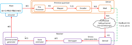
Figure 1: A typical architecture of a networked control system.

II System Model

Fig. 1 shows a typical networked control system (NCS), which consists of a plant, a sensor, and a controller, and they form a closed-loop control. We consider a slotted system, where the time dimension is partitioned into decision slots indexed by $t$ with duration $\tau$. The sensor has perfect state observation of the plant state $\mathbf{x}(t)$. The controller is geographically separated from the sensor, and there is a temporally correlated wireless fading channel connecting them. At each time slot $t$, the sensor observes the plant state and the pre-processor generates $\mathbf{i}(t)$, which is passed to the mapper. The mapper maps $\mathbf{i}(t)$ to one of the $M=2^{R}$ quantization levels $\boldsymbol{\xi}(t)$, which is encodes into $R$-digit binary information bits at the encoder. The information bits are communicated to the remote controller over the wireless fading channel using $M$ quadrature amplitude modulation (MQAM). Specifically, the $R$-digit binary information bits are mapped to one of the $M$ available QAM symbols for a given constellation type. After the demodulation process, the demodulator outputs binary information bits to the demapper, which maps the information bits back to one of the $M$ quantization levels $\mathbf{y}(t)$. Then, $\mathbf{y}(t)$ is passed to the state estimator to obtain a state estimate $\hat{\mathbf{x}}(t)$. After that, $\hat{\mathbf{x}}(t)$ is passed to the actuator to generate a control action $\mathbf{u}(t)$. The actuator, which is co-located with the plant, uses control action $\mathbf{u}(t)$ for plant actuation.

Such an NCS with a wireless fading channel covers a lot of practical applications. For example, in a heating, ventilation and air conditioning (HVAC) system [20], the boiler and chiller components (i.e., the controller) of the HVAC system are mounted on the rooftop. The temperature and humidity sensors are located inside a room, which measure certain indoor environmental parameters and transmit the data to the controller over a wireless channel. The controller then decides whether to pump cool or hot air into the room through the ducts based on the received data.

II-A Linear Stochastic Plant Model

We consider a continuous-time stochastic plant system with dynamics $\frac{d{\mathbf{x}}(t)}{dt}=\widetilde{\mathbf{F}}\mathbf{x}(t)+\widetilde{\mathbf{G}}\mathbf{u}(t)+\widetilde{\mathbf{w}}(t)$, $t\geq 0$, $\mathbf{x}(0)=\mathbf{x}_{0}$, where $\mathbf{x}(t)\in\mathbb{R}^{d}$ is the plant state, $\mathbf{u}(t)\in\mathbb{R}^{m}$ is the plant control action, $\mathbf{x}_{0}$ is the initial plant state, $\widetilde{\mathbf{F}}\in\mathbb{R}^{d\times d}$, $\widetilde{\mathbf{G}}\in\mathbb{R}^{d\times m}$, and $\widetilde{\mathbf{w}}(t)\in\mathbb{R}^{d}$ is an additive plant disturbance with zero mean and covariance $\widetilde{\mathbf{W}}\in\mathbb{R}^{d\times d}$. Furthermore, we assume that the plant disturbance is bounded, i.e., $\|\widetilde{\mathbf{w}}(t)\|\leq\widetilde{w}_{max}$ for some $\widetilde{w}_{max}>0$ [21], [22]. Without loss of generality, we assume that $\widetilde{\mathbf{W}}$ is diagonal. Since the sensor in the NCS samples the plant state once per time slot (with duration $\tau$), the state dynamics of the sampled discrete-time stochastic plant system is given by [23]

$$\mathbf{x}(t+1)=\mathbf{F}\mathbf{x}(t)+\mathbf{G}\mathbf{u}(t)+\mathbf{w}(t),\ \mathbf{x}(0)=\mathbf{x}_{0}$$ (1)

for $t\geq 0$, where $\mathbf{F}=\exp(\widetilde{\mathbf{F}}\tau)$, $\mathbf{G}=\widetilde{\mathbf{F}}^{-1}\big{(}\exp(\widetilde{\mathbf{F}}\tau)-\mathbf{I}\big{)}\widetilde{\mathbf{G}}$, and $\mathbf{w}(t)=\int_{0}^{\tau}\exp(\widetilde{\mathbf{F}}s)\widetilde{\mathbf{w}}((t+1)\tau-s)ds$ is an i.i.d. random noise with zero mean and covariance $\mathbf{W}=\int_{0}^{\tau}\exp(\widetilde{\mathbf{F}}s)\widetilde{\mathbf{W}}\exp(\widetilde{\mathbf{F}}s)ds$. We have the following assumptions on the plant model:

Assumption 1 (Stochastic Plant Model).

We assume that the plant system $\big{(}\mathbf{F},\mathbf{G}\big{)}$ in (1) is controllable [2]. Furthermore, we assume that the initial condition in (1) is bounded, i.e., $\|\mathbf{x}_{0}\|\leq L$ and $L=\mathcal{O}(\tau)$.  ∎

II-B Wireless Fading Channel Model

We consider a continuous-time temporally correlated wireless fading channel with dynamics $\frac{dh(t)}{dt}=-\widetilde{a}h(t)+\sqrt{2\widetilde{a}}\widetilde{z}(t)$, $t\geq 0$, with $h(0)=h_{0}$, where $h(t)\in\mathbb{C}$ is the channel state information (CSI) and $h_{0}$ is the initial channel state. The coefficient $\widetilde{a}\in\mathbb{R}^{+}$ determines the temporal correlation of the fading process and $\widetilde{z}(t)\sim\mathcal{CN}(0,1)$ is an additive circularly-symmetric Gaussian noise with zero mean and unit variance. Similarly, the state dynamics of the sampled discrete-time channel is given by [23]

$$h(t+1)=ah(t)+z(t),\quad h(0)=h_{0}$$ (2)

for $t\geq 0$, where $a=\exp(-\widetilde{a}\tau)$ and $z(t)=\sqrt{2\widetilde{a}}\int_{0}^{\tau}\exp(-\widetilde{a}\tau)\widetilde{z}((t+1)\tau-s)ds$ is an i.i.d. noise with zero mean and covariance $Z=1-\exp(-2\widetilde{a}\tau)$. The received signal at the demodulator of the controller is given by

$$\mathbf{r}(t)=\sqrt{p(t)}h(t)\mathbf{b}(t)+\mathbf{n}(t)$$ (3)

where $p(t)\in\mathbb{R}^{+}$ is the transmit SNR and $\mathbf{n}(t)\sim\mathcal{CN}(0,\mathbf{I})$ is an i.i.d. Gaussian noise. Let $\gamma(t)\in\{0,1\}$ denote the symbol error event (where $\gamma(t)=0$ means symbol error). In this paper, we consider rectangular MQAM constellation (e.g., [18], [26], [27]), and the associated symbol error rate (SER) is given by

$$\Pr\left[\gamma(t)=0\right]\approx\exp\Big{(}-\frac{p(t)\tau\big{|}h(t)\big{|}^{2}}{\kappa(R)B_{W}}\Big{)}$$ (4)

where $B_{W}$ is the channel bandwidth and $\kappa(R)=\frac{2^{R+1}-2}{3}$ is a constant. The received signal is processed in the demodulator, which outputs information bits to the reconstructor. The reconstructor maps the information bits back to one of the $M$ quantization levels and the associated output $\mathbf{y}(t)$ is given by

$$\mathbf{y}(t)=\gamma(t)\boldsymbol{\xi}(t)$$ (5)

Note that $\boldsymbol{\xi}(t)$ is the the output of the mapper at the sensor. Furthermore, (5) means that $\mathbf{y}(t)=\boldsymbol{\xi}(t)$ for successful transmission and $\mathbf{y}(t)=\mathbf{0}$ otherwise.

II-C Information Structures at the Sensor and the Controller

Let $a_{0}^{t}\triangleq\left\{a(s):0\leq s\leq t\right\}$ be the history of realizations of variable $a$ up to time $t$. The available knowledge at the sensor and the controller at time $t$ are represented by the information structures $I_{S}(t)$ and $I_{C}(t)$. Specifically, $I_{S}(t)$ is given by

$$I_{S}(t) =\big{\{}\underbrace{\mathbf{x}_{0}^{t},\mathbf{i}_{0}^{t},\mathbf{u}_{0}^{t-1}}_{\text{control-related states}},\underbrace{\boldsymbol{\xi}_{0}^{t},\alpha_{0}^{t-1},\gamma_{0}^{t-1}}_{\text{com.-related states}}\big{\}}$$ (6)

for $t>0$, and $I_{S}(0)=\left\{\mathbf{x}(0),\mathbf{i}(0),\boldsymbol{\xi}(0)\right\}$, where we denote $\alpha(t)=|h(t)|^{2}$ ($\forall t$). Moreover, $I_{C}(t)$ is given by

$$I_{C}(t)=\big{\{}\underbrace{\mathbf{u}_{0}^{t-1}}_{\text{control-related states}},\underbrace{\alpha_{0}^{t},\gamma_{0}^{\nu(t)},\mathbf{y}_{0}^{\nu(t)}}_{\text{com.-related states}}\big{\}}$$ (7)

for $t>0$, and $I_{C}(0)=\left\{\alpha(0),\gamma(\nu(0)),y(\nu(0))\right\}$, where $\nu(t)=\max\{s\leq t:\gamma(s)=1\}$ is the slot of the latest successful transmission by time $t$. Note that at time slot $t$, the sensor discards the events of the form $\gamma(t)=0$. We have the following observations on $I_{S}(t)$ and $I_{C}(t)$:

Remark 1 (Observations on $I_{S}(t)$ and $I_{C}(t)$).

• For $I_{S}(t)$, $\mathbf{x}_{0}^{t}$ is the plant state, $\mathbf{i}_{0}^{t}$ is the pre-processor output, $\mathbf{u}_{0}^{t-1}$ is the plant control action, $\boldsymbol{\xi}_{0}^{t}$ is the mapper output, and all can be locally obtained at the sensor. The information $\left\{\alpha_{0}^{t-1},\gamma_{0}^{t-1}\right\}$ can be obtained by the feedback signals from the controller as shown in Fig. 1.

• For $I_{C}(t)$, $\mathbf{u}_{0}^{t-1}$ is the locally generated plant control action, $\alpha_{0}^{t}$ can be locally measured using the pilots from the sensor [28], and $\{\gamma_{0}^{\nu(t)},\mathbf{y}_{0}^{\nu(t)}\}$ are the symbol error indicators and the received signals, which are the output of the wireless fading channel and can be locally obtained at the controller.

• There is an intersection of $I_{S}(t)$ and $I_{C}(t)$, which is denoted as $I_{SC}(t)\triangleq I_{S}(t)\cap I_{C}(t)$. Specifically, $I_{SC}(t)=\{\mathbf{u}_{0}^{t-1},\alpha_{0}^{t-1},{\color[rgb]{0,0,0}\gamma_{0}^{\nu(t-1)},\mathbf{y}_{0}^{\nu(t-1)}}\}$ for $t>0$, and $I_{SC}(0)=\emptyset$.   ∎

II-D Communication Power and Plant Control Policies

Based on $I_{S}(t)$ and $I_{C}(t)$, we define the communication power and plant control policies. Let $\mathcal{F}_{S}(t)=\sigma\left(\left\{I_{S}(s):0\leq s\leq t\right\}\right)$ be the minimal $\sigma$-algebra containing the set $\left\{I_{S}(s):0\leq s\leq t\right\}$ and $\left\{\mathcal{F}_{S}(t)\right\}$ be the associated filtration at the sensor. Similarly, define $\mathcal{F}_{C}(t)=\sigma\left(\left\{I_{C}(s):0\leq s\leq t\right\}\right)$ and let $\left\{\mathcal{F}_{C}(t)\right\}$ be the associated filtration at the controller. At the beginning of time slot $t$, the sensor determines the power control action $p(t)$ and the controller determines the plant control action $\mathbf{u}(t)$ according to the following control policies:

Definition 1 (Plant Control Policy).

A plant control policy $\Omega_{\mathbf{u}}$ at the controller is $\mathcal{F}_{C}(t)$-adapted, meaning that $\mathbf{u}(t)$ is adaptive to all the information $I_{C}(s)$ up to time slot $t$ (i.e., $\left\{I_{C}(s):0\leq s\leq t\right\}$).   ∎

Definition 2 (Communication Power Control Policy).

A communication power control policy $\Omega_{p}$ at the sensor is $\mathcal{F}_{S}(t)$-adapted, meaning that $p(t)$ is adaptive to all the information $I_{S}(s)$ up to time slot $t$ (i.e., $\left\{I_{S}(s):0\leq s\leq t\right\}$). Furthermore, $\Omega_{p}$ satisfies the peak power constraint, i.e., $p(t)\in\left[0,p_{max}\right]$ for all $t$, where $p_{max}>0$ is the maximum power the sensor can use at each time slot.   ∎

Remark 2 (Interpretation of the Power Control Policy).

The power control policy in Definition 2 is an error-adaptive power control. In such strategy, the rate of the channel $R$ is fixed, which means that the constellation size of the MQAM (where $M=2^{R}$) is unchanged during the communication session. At each time slot $t$, the sensor controls the communication power $p(t)$ to dynamically adjust the SER in (4), so that the state estimation error at the controller is adjusted. Hence, there is an inherent tradeoff between the plant performance (in the stability or optimal control sense) and the communication cost (in terms of the average transmit power). We shall quantify this tradeoff in the following sections.    ∎

III Communication Power Problem Formulation

In this section, we first introduce a primitive quantizer at the sensor. We then establish the no dual effect property under such a quantizer and give the optimal plant control policy w.r.t. the joint communication power and plant control problem. Based on the primitive quantizer and the CE controller, we formally formulate the communication power problem.

III-A Primitive Quantizer

Following [3] and [5], we adopt a primitive quantizer at the sensor to track the dynamic range of the plant state. Specifically, the primitive quantizer is characterized by four parameters $\left(\widetilde{\mathbf{x}},\boldsymbol{\Psi},\mathbf{L},\mathbf{R}\right)$, where $\widetilde{\mathbf{x}}(t)\triangleq\mathbb{E}\left[\mathbf{x}(t)\big{|}I_{SC}(t)\right]\in\mathbb{R}^{d}$ is the shifting vector, $\boldsymbol{\Psi}(t)\in\mathbb{R}^{d\times d}$ is the coordinate transformation matrix, $\mathbf{L}(t)=(L_{1}(t),\dots,L_{d}(t))^{T}\in\mathbb{R}^{d}$ is the dynamic range, and $\mathbf{R}=(R_{1},\dots,R_{d})^{T}\in\mathbb{R}^{d}$ is the rate vector with $\sum_{n=1}^{d}R_{n}=R$ (where $R_{n}$ determines the quantization level of the $n$-th element of the plant state $\mathbf{x}$).

The primitive quantizer consists of three components, i.e., a pre-processor, a mapper and an encoder. Specifically, the pre-processor takes $\mathbf{x}(t)$ as input and generates the innovation $\mathbf{i}(t)=\mathbf{x}(t)-\widetilde{\mathbf{x}}(t)$, which is passed to the mapper. The mapper maps $\boldsymbol{\Psi}(t)\mathbf{i}(t)$ to one of the $M=2^{R}$ quantization levels within the region $\big{\{}[-L_{1}(t),L_{1}(t)]\times\cdots\times[-L_{d}(t),L_{d}(t)]\big{\}}$ and outputs $\boldsymbol{\xi}(t)$. Then $\boldsymbol{\xi}(t)$ is encoded into $R$-digit binary information bits. Please refer to Appendix A on how the primitive quantizer works in detail. We summarize the property of the primitive quantizer as follows:

Lemma 1 (Properties of the Primitive Quantizer).

• The primitive quantizer tracks the dynamic range of the plant state $\mathbf{x}(t)$, i.e.,

  $$\mathbf{x}(t)\in\big{\{}\mathbf{x}\in\mathbb{R}^{d}:\boldsymbol{\Psi}(t)\big{(}\mathbf{x}-\widetilde{\mathbf{x}}(t)\big{)}$$

  $$\in\left\{[-L_{1}(t),L_{1}(t)]\times\cdots\times[-L_{d}(t),L_{d}(t)]\right\}\big{\}},\ \forall t$$ (8)

• The equivalent model between input $\mathbf{x}(t)$ and mapper output $\boldsymbol{\xi}(t)$ can be expressed as

  $$\boldsymbol{\xi}(t)=\boldsymbol{\Psi}(t)\big{(}\mathbf{x}(t)-\widetilde{\mathbf{x}}(t)\big{)}+\mathbf{e}(\mathbf{L}(t),t)$$ (9)

  where $\mathbf{e}(\mathbf{L}(t),t)=\big{(}e_{1}(L_{1}(t),t),\dots,e_{d}(L_{d}(t),t)\big{)}^{T}\in\mathbb{R}^{d}$ is the quantization noise, and for each $n$, $e_{n}(L_{n}(t),t)$ is uniformly distributed within the region $\big{[}-\frac{L_{n}(t)}{2^{R_{n}-1}},\frac{L_{n}(t)}{2^{R_{n}-1}}\big{]}$.    ∎

Therefore, according to (8), we can use the primitive quantizer to track the dynamic range of the plant state $\mathbf{x}(t)$.

III-B Certainty Equivalent Controller

As in [9] and [17], we consider the following joint communication power and plant control optimization problem:

$$\min_{\Omega_{\mathbf{u}},\Omega_{p}}\ \limsup_{T\rightarrow\infty}\frac{1}{T} \sum_{t=0}^{T-1}\mathbb{E}^{\Omega_{\mathbf{u}},\Omega_{p}}\big{[}\mathbf{x}^{T}(t)\mathbf{Q}\mathbf{x}(t)+\mathbf{u}^{T}(t)\mathbf{D}\mathbf{u}(t)+\lambda p(t)\big{]}$$

where $\mathbf{Q}$ and $\mathbf{D}$ are positive definite symmetric weighting matrices for the plant state deviation cost and the plant control cost, and $\lambda\in\mathbb{R}^{+}$ is the communication power price. In general, the design of the communication power policy and the plant control policy are coupled together. This is because the communication power will affect the state estimation accuracy at the controller, which will in turn affect the plant state evolution. However, by establishing the no dual effect property (e.g., [4], [19]), we can obtain the optimal plant control policy for the above joint optimization problem. Specifically, let $\hat{\mathbf{x}}(t)=\mathbb{E}\big{[}\mathbf{x}(t)\big{|}I_{C}(t)\big{]}$ be the plant state estimate at the controller and $\boldsymbol{\Delta}(t)=\mathbf{x}(t)-\hat{\mathbf{x}}(t)$ be the state estimation error. The no dual effect property is established as follows:

Lemma 2 (No Dual Effect Property).

Under the primitive quantizer in Section III-A, we have the following no dual effect property in our NCS:

$$\mathbb{E}\big{[}\boldsymbol{\Delta}^{T}(t)\boldsymbol{\Delta}(t)\big{|}I_{C}(t)\big{]}=\mathbb{E}\big{[}\boldsymbol{\Delta}^{T}(t)\boldsymbol{\Delta}(t)\big{|}\alpha_{0}^{t},\gamma_{0}^{\nu(t)},\mathbf{y}_{0}^{\nu(t)}\big{]},\quad\forall t$$

Proof.

please refer to Appendix B. ∎

Using the no dual effect property in Lemma 2 and Prop. 3.1 of [4] (or Theorem 1 in Section III of [19]), the optimal plant control policy is given by the certainty equivalent (CE) controller:

$$\Omega_{\mathbf{u}}^{\ast}\big{(}I_{C}(t)\big{)}=\mathbf{u}^{\ast}(t),\quad\text{where }\mathbf{u}^{\ast}(t)=-\mathbf{K}\hat{\mathbf{x}}(t),\quad\forall t$$ (10)

where $\mathbf{K}=(\mathbf{G}^{T}\mathbf{P}\mathbf{G}+\mathbf{D})^{-1}\mathbf{G}^{T}\mathbf{P}\mathbf{F}$ is the feedback gain matrix, and $\mathbf{P}$ satisfies the following discrete time algebraic Riccati equation (DARE): $\mathbf{P}=\mathbf{F}^{T}\mathbf{P}\mathbf{F}-\mathbf{F}^{T}\mathbf{P}\mathbf{G}(\mathbf{G}^{T}\mathbf{P}\mathbf{G}+\mathbf{D})^{-1}\mathbf{G}^{T}\mathbf{P}\mathbf{F}+\mathbf{W}$.

III-C Communication Power Problem Formulation

Under the primitive quantizer and the CE controller, the per-stage state estimation error and communication power cost is given by

$$c\big{(}\boldsymbol{\Delta}(t),p(t)\big{)}=\boldsymbol{\Delta}^{T}(t)\mathbf{S}\boldsymbol{\Delta}(t)+\lambda p(t)$$ (11)

where $\mathbf{S}$ is a positive definite symmetric weighting matrix. We consider the following communication power optimization problem:

Problem 1.

(Communication Power Optimization Problem):

$$\min_{\Omega_{p}}\quad \limsup_{T\rightarrow\infty}\ \frac{1}{T}\sum_{t=0}^{T-1}\mathbb{E}^{\Omega_{\mathbf{u}}^{\ast},\Omega_{p}}\left[c\big{(}\boldsymbol{\Delta}(t),p(t)\big{)}\right]$$ (12)

where $\boldsymbol{\Delta}(t)$ has the following dynamics:

$$\boldsymbol{\Delta}(t)=\left\{\begin{aligned} &\mathbf{F}\boldsymbol{\Delta}(t-1)+\mathbf{w}(t-1),\quad&\text{if }\gamma(t)=0\\ &-\boldsymbol{\Psi}^{-1}(t)\mathbf{e}(\mathbf{L}(t),t),\quad&\text{if }\gamma(t)=1\end{aligned}\right.$$ (13)

where $\mathbf{e}(\mathbf{L}(t),t)$ is the quantization noise in (9).  ∎

We need to design a communication power control policy such that the plant system and the primitive are stable, and state estimation error is bounded. Specifically, we have the following definition on the admissible communication power control policy of the NCS under the CE controller $\Omega_{\mathbf{u}}^{\ast}$ in (10):

Definition 3.

(Admissible Communication Power Control Policy): A communication power control policy $\Omega_{p}$ of the NCS is admissible if,

• The plant state process $\left\{\mathbf{x}\left(t\right)\right\}$ is stable in the sense that $\lim_{t\rightarrow\infty}\mathbb{E}^{\Omega_{\mathbf{u}}^{\ast},\Omega_{p}}\big{[}\left\|\mathbf{x}(t)\right\|^{2}\big{]}<\infty$, where $\mathbb{E}^{\Omega_{p},\Omega_{\mathbf{u}}}$ means taking expectation w.r.t. the probability measure induced by $\left(\Omega_{\mathbf{u}}^{\ast},\Omega_{p}\right)$.

• The dynamic range of the quantizer $\left\{\mathbf{L}(t)\right\}$ is stable in the sense that $\lim_{t\rightarrow\infty}\mathbb{E}^{\Omega_{\mathbf{u}}^{\ast},\Omega_{p}}\big{[}\left\|\mathbf{L}(t)\right\|^{2}\big{]}<\infty$.

• The process $\left\{\boldsymbol{\Delta}(t)\right\}$ at the sensor is stable in the sense that $\lim_{t\rightarrow\infty}\mathbb{E}^{\Omega_{\mathbf{u}}^{\ast}\Omega_{p}}\big{[}\left\|\boldsymbol{\Delta}(t)\right\|^{2}\big{]}<\infty$.   ∎

Problem 1 is an MDP and we show in Appendix C that it is without loss of optimality that we restrict the system state to be $\boldsymbol{\chi}(t)\triangleq\big{\{}\boldsymbol{\Delta}(t-1),\alpha(t-1),\boldsymbol{\Psi}(t),\mathbf{L}(t)\big{\}}\in\sigma\left(\left\{I_{S}(s):0\leq s\leq t\right\}\right)$ with transition kernel $\Pr\big{[}\boldsymbol{\chi}(t+1)\big{|}\boldsymbol{\chi}(t),p(t)\big{]}$. Using dynamic programming theories [12], the optimality conditions of Problem 1 are given as follows:

Theorem 1 (Sufficient Conditions for Optimality).

If there exists $\left(\theta^{\ast},V^{\ast}(\boldsymbol{\chi})\right)$ that satisfies the following optimality equation (Bellman equation):

$$\theta^{\ast}\tau+V^{\ast}\left(\boldsymbol{\chi}\right)= \min_{p\in\Omega_{p}(\boldsymbol{\chi})}\mathbb{E}\big{[}\big{(}(\boldsymbol{\Delta}^{\prime})^{T}\mathbf{S}(\boldsymbol{\Delta}^{\prime})+\lambda p\big{)}\tau$$

$$+\sum_{\boldsymbol{\chi}^{\prime}}\Pr\left[\boldsymbol{\chi}^{\prime}\big{|}\boldsymbol{\chi},p\right]V^{\ast}\left(\boldsymbol{\chi}^{\prime}\right)\big{|}\boldsymbol{\chi}\big{]},\quad\forall\boldsymbol{\chi}$$ (14)

and for all admissible communication power control policies $\Omega_{p}$, $V^{\ast}(\boldsymbol{\chi})$ satisfies the following transversality condition:

$$\lim_{T\rightarrow\infty}\frac{1}{T}\mathbb{E}^{\Omega_{p}}\left[V^{\ast}\left(\boldsymbol{\chi}\left(T\right)\right)|\boldsymbol{\chi}\left(0\right)\right]=0$$ (15)

Then, we have the following results:

• $\theta^{\ast}=\min_{\Omega_{p}}\limsup_{T\rightarrow\infty}\frac{1}{T}\sum_{t=0}^{T-1}\mathbb{E}^{\Omega_{\mathbf{u}}^{\ast},\Omega_{p}}\left[c\big{(}\boldsymbol{\Delta}(t),p(t)\big{)}\right]$ is the optimal average cost of Problem 1.

• Suppose there exists an admissible communication power control policy $\Omega_{p}^{\ast}$ with $\Omega_{p}^{*}\left(\boldsymbol{\chi}\right)=p^{\ast}$, where $p^{\ast}$ attains the minimum of the R.H.S. in (14) for given $\boldsymbol{\chi}$. Then, the optimal communication power policy of Problem 1 is given by a stationary Markovian policy $\Omega_{p}^{\ast}$.

Proof.

please refer to Appendix C. ∎

Unfortunately, the Bellman equation in (14) is very difficult to solve because it involves a huge number of fixed point equations w.r.t. $\left(\theta^{\ast},V^{\ast}(\boldsymbol{\chi})\right)$. Numerical solutions such as numerical VIA [12], [29] have exponential complexity w.r.t. $d^{2}$, where $d$ is the dimension of the plant state $\mathbf{x}$).

In Section IV, we shall derive a closed-form approximation for $V(\boldsymbol{\chi})$ using continuous-time perturbation techniques.

IV Low Complexity Power Control Solution

In this section, we first adopt a continuous-time perturbation approach to analyze the difference between a closed-form approximate value function and the optimal value function. We analyze the performance gap between the policy obtained from the continuous-time perturbation approach and the optimal control policy. Then, we focus on deriving the closed-form approximate value function and proposing a low complexity power control scheme. We also give sufficient conditions for the NCS stability.

IV-A Continuous-Time Approximation

We first have the following theorem for solving the optimality equation in (14) using continuous-time perturbation analysis [30], [31]:

Lemma 3.

(Perturbation Analysis for Solving the Optimality Equation): If there exists $\left(\theta,V(\boldsymbol{\chi})\right)$ where $V\in\mathcal{C}^{2}$ that satisfies

• the following multi-dimensional PDE:

  $$\theta=\boldsymbol{\Delta}^{T}\mathbf{S}\boldsymbol{\Delta}$$ (16)

  $$+\min_{0\leq p\leq p_{max}}\big{[}\lambda+\left(V(\boldsymbol{\chi})\big{|}_{\boldsymbol{\Delta}=\mathbf{0}}-V(\boldsymbol{\chi})\right)\frac{\alpha}{\kappa(R)B_{W}}\big{]}p$$

  $$+\nabla_{\boldsymbol{\Delta}}^{T}V(\boldsymbol{\chi})\widetilde{\mathbf{F}}\boldsymbol{\Delta}+\frac{1}{2}\text{Tr}\left(\nabla_{\boldsymbol{\Delta}}^{2}V(\boldsymbol{\chi})\widetilde{\mathbf{W}}\right)$$

  $$+\frac{\partial V(\boldsymbol{\chi})}{\partial\alpha}\left(2\widetilde{a}\alpha+2\widetilde{a}\right)+\frac{\partial^{2}V^{\ast}(\boldsymbol{\chi})}{\partial\alpha^{2}}4\widetilde{a}\alpha$$

  $$+\text{Tr}\Big{(}\frac{\partial V(\boldsymbol{\chi})}{\partial\boldsymbol{\Psi}}(\mathbf{H}\boldsymbol{\Psi}-\boldsymbol{\Psi})/\tau\Big{)}$$

  $$+\nabla^{T}_{\mathbf{L}}V(\boldsymbol{\chi})\big{(}\boldsymbol{\Gamma}\mathbf{F}_{\mathbf{R}}\mathbf{L}+w_{max}\|\mathbf{H}\boldsymbol{\Psi}\|\mathbf{1}-\mathbf{L}\big{)}/\tau$$

• and $V(\boldsymbol{\chi})=\mathcal{O}(\left\|\boldsymbol{\Delta}\right\|^{2})$.

Then, for any $\boldsymbol{\chi}$,

$$V^{\ast}\left(\boldsymbol{\chi}\right)=V(\boldsymbol{\chi})+\mathcal{O}\left(\tau\right)+{\color[rgb]{0,0,0}\mathcal{O}\Big{(}\frac{\tau^{2}}{2^{2R_{min}}}\Big{)}}$$ (17)

as $\tau\rightarrow 0$, where $R_{min}=\min\{R_{n}:\forall n\}$, and $\mathcal{O}\left(\tau\right)$ and $\mathcal{O}\big{(}\frac{\tau^{2}}{2^{2R_{min}}}\big{)}$ are the error terms due to the continuous time approximation and the quantization, respectively. Furthermore, $V(\boldsymbol{\chi})$ satisfies the transversality condition in (15).

Proof.

please refer to Appendix D. ∎

As a result, solving the optimality equation in (14) is transformed into a calculus problem of solving the PDE in (16), and the difference between $V(\boldsymbol{\chi})$ and $V^{\ast}(\boldsymbol{\chi})$ is $\mathcal{O}\left(\tau\right)+\mathcal{O}\big{(}\frac{\tau^{2}}{2^{2R_{min}}}\big{)}$ for sufficiently small $\tau$.

Let $\widetilde{\Omega}_{p}^{\ast}$ be the control policy, under which the generated control action achieves the minimization in the PDE in (16) for any $\boldsymbol{\chi}$. Let $\widetilde{\theta}^{\ast}=\limsup_{T\rightarrow\infty}\frac{1}{T}\sum_{t=0}^{T-1}\mathbb{E}^{\Omega_{\mathbf{u}}^{\ast},\widetilde{\Omega}_{p}^{\ast}}\big{[}c\big{(}\boldsymbol{\Delta}(t),p(t)\big{)}\big{]}$ be the associated performance. The gap between $\widetilde{\theta}^{\ast}$ and the optimal average cost $\theta^{\ast}$ in (14) is established as follows:

Theorem 2 (Performance Gap between $\widetilde{\theta}^{\ast}$ and $\theta^{\ast}$).

If $V(\boldsymbol{\chi})=\mathcal{O}(\left\|\boldsymbol{\Delta}\right\|^{2})$ and $\widetilde{\Omega}_{p}^{\ast}$ is admissible, we have

$$\widetilde{\theta}^{\ast}-\theta^{\ast}=\mathcal{O}(\tau)+\mathcal{O}\Big{(}\frac{\tau^{2}}{2^{2R_{min}}}\Big{)}$$ (18)

as $\tau\rightarrow 0$.

Proof.

Please refer to Appendix E. ∎

Theorem 2 suggests that $\widetilde{\theta}^{\ast}\rightarrow\theta^{\ast}$ as $\tau\rightarrow 0$. In other words, the power control policy $\widetilde{\Omega}_{p}^{\ast}$ is asymptotically optimal for sufficiently small $\tau$.

IV-B Closed-Form Approximate Value Function

In this subsection, we solve the PDE in (16) to obtain the closed-form approximate value function $V(\boldsymbol{\chi})$. It can be observed that the PDE in (16) is multi-dimensional and coupled in the variables $(\boldsymbol{\Delta},\alpha,\boldsymbol{\Psi},\mathbf{L})$, and it is quite challenging to obtain the closed-form solution. In the following Lemma, we derive an asymptotic solution of the PDE using the asymptotic expansion technique [31].

Lemma 4 (Asymptotic Solution of the PDE).

The asymptotic solution of the PDE in (16) is given as follows:

• for small $\|\boldsymbol{\Delta}\|^{2}\alpha$ (Bad Transmission Opportunity/Low Urgency Regime),

  $$\log\left(V(\boldsymbol{\chi})\right)=\log(\boldsymbol{\Delta}^{T}A_{1,\mathbf{U}}(\alpha)\boldsymbol{\Delta}+b_{1}(\alpha))+\mathcal{O}\left({\alpha}\right)$$ (19)

  where $A_{1,\mathbf{U}}(\alpha)\in\mathbb{R}^{d\times d}$ and $b_{1}(\alpha)\in\mathbb{R}$ are given in (76) in Appendix F.

• for large $\|\boldsymbol{\Delta}\|^{2}\alpha$ (Good Transmission Opportunity/High Urgency Regime),

  $$\log\left(V(\boldsymbol{\chi})\right)=\log(\boldsymbol{\Delta}^{T}A_{2,\mathbf{U}}(\alpha)\boldsymbol{\Delta}+\exp\left(2B_{2}\right)\alpha^{C_{2}})$$

  $$-\frac{\widetilde{a}-\widetilde{c}}{4}\alpha-\big{(}\frac{1}{4}-\frac{\widetilde{a}}{4\widetilde{c}}\big{)}\log\alpha+\mathcal{O}\big{(}\frac{1}{\alpha\sqrt{p_{max}}}\big{)}$$ (20)

  where $A_{2,\mathbf{U}}(\alpha)\in\mathbb{R}^{d\times d}$ and $B_{2}\in\mathbb{R}$ are given in (81) in Appendix F.

Proof.

please refer to Appendix F. ∎

Based on Lemma 4, we adopt the following approximation for the solution of the PDE in (16):

$$\log\left(V(\boldsymbol{\chi})\right)\approx{\color[rgb]{0,0,0}\log\big{(}\widetilde{V}_{\eta_{th}}(\boldsymbol{\chi})\big{)}}$$

$$\triangleq \left\{\begin{aligned} &\log(\boldsymbol{\Delta}^{T}A_{1,\mathbf{U}}(\alpha)\boldsymbol{\Delta}+b_{1}(\alpha)),\text{for }\|\boldsymbol{\Delta}\|^{2}\alpha<\eta_{th}\\ &\log(\boldsymbol{\Delta}^{T}A_{2,\mathbf{U}}(\alpha)\boldsymbol{\Delta}+\exp\left(2B_{2}\right)\alpha^{C_{2}})-\frac{\widetilde{a}-\widetilde{c}}{4}\alpha\\ &-\left(\frac{1}{4}-\frac{\widetilde{a}}{4\widetilde{c}}\right)\log\alpha,\hskip 2.84544pt\text{for }\|\boldsymbol{\Delta}\|^{2}\alpha\geq\eta_{th}\end{aligned}\right.$$ (21)

where $\eta_{th}>0$ is a solution parameter.

IV-C Structural Properties of the Low Complexity Power Control

Using Lemma 3 and (LABEL:approxvaluefunc), we obtain a low complexity power control policy in the following theorem:

Theorem 3 (Structural Properties of Power Control Policy).

The optimizing power control policy $\widetilde{\Omega}_{p}^{\ast}$ that minimize the R.H.S. of the PDE in (16) is given by

$$\widetilde{\Omega}_{p}^{\ast}\left(\boldsymbol{\chi}\right)=p^{\ast}$$ (22)

$$= \left\{\begin{aligned} &0,\ \text{if }\lambda>{\color[rgb]{0,0,0}\big{(}\widetilde{V}_{\eta_{th}}(\boldsymbol{\chi})-\widetilde{V}_{\eta_{th}}(\boldsymbol{\chi})\big{|}_{\boldsymbol{\Delta}=\mathbf{0}}\big{)}\frac{\alpha}{\kappa(R)B_{W}}}\\ &p_{max},\ \text{if }\lambda\leq{\color[rgb]{0,0,0}\big{(}\widetilde{V}_{\eta_{th}}(\boldsymbol{\chi})-\widetilde{V}_{\eta_{th}}(\boldsymbol{\chi})\big{|}_{\boldsymbol{\Delta}=\mathbf{0}}\big{)}\frac{\alpha}{\kappa(R)B_{W}}}\end{aligned}\right.$$

∎

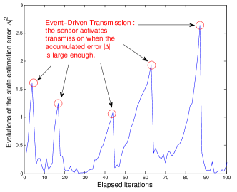
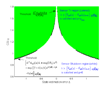
Figure 2: (a) Evolutions of $\|\boldsymbol{\Delta}(t)\|^{2}$ under $\widetilde{\Omega}_{p}^{\ast}$. (b) Decision region (sensor shutdown/Tx region) under $\widetilde{\Omega}_{p}^{\ast}$. The system parameters are configured as in Fig. 4, and $\widetilde{\mathbf{F}}=-3$ with system state dimension $L=1$, $\lambda=2000$, and $\eta_{th}=0.43$ (which is determined according to the method in Fig. 3).

It can be observed that the power control policy $\widetilde{\Omega}_{p}^{\ast}$ has an event-driven control structure with a dynamically changing threshold ${\color[rgb]{0,0,0}\big{(}\widetilde{V}_{\eta_{th}}(\boldsymbol{\chi})-\widetilde{V}_{\eta_{th}}(\boldsymbol{\chi})\big{|}_{\boldsymbol{\Delta}=\mathbf{0}}\big{)}\frac{\alpha}{\kappa(R)B_{W}}}$. Specifically, the sensor either transmits using the maximum power or shots down depending whether the dynamic threshold is larger than $\lambda$ or not. Fig. 2(a) illustrates a sample path of the state estimation error $\boldsymbol{\Delta}(t)$ and it can be observed that the sensor only activates transmission when the accumulated error is large enough. Furthermore, the dynamic threshold is adaptive to the plant state estimation error $\boldsymbol{\Delta}$ and the CSI $\alpha$. Using the approximate value function in (LABEL:approxvaluefunc), we have the following discussions on the dynamic threshold:

Remark 3 (Properties of the Dynamic Threshold).

The dynamic threshold is affected by the following factors:

• Dynamic Threshold w.r.t. $\boldsymbol{\Delta}$: For given CSI $\alpha$ and data rate $R$, the dynamic threshold increases w.r.t. the state estimation error $\boldsymbol{\Delta}$ at the order of $\mathcal{O}(\|\boldsymbol{\Delta}\|^{2})$. This means that large state estimation error $\|\boldsymbol{\Delta}\|$ tends to use full power. This is reasonable because large state estimation error means the urgency of delivering information to the controller, which leads to use large power.

• Dynamic Threshold w.r.t. $\alpha$: For given state estimation error $\boldsymbol{\Delta}$ and data rate $R$, the dynamic threshold increases w.r.t. the CSI $\alpha$ at the order of $\mathcal{O}(\exp(\alpha))$. This means that large CSI $\alpha$ tends to use full power. Note that large $\alpha$ means good transmission opportunities. Hence, it is reasonable to use more power to reduce the SER.

• Dynamic Threshold w.r.t. $R$: For given large CSI $\alpha$ or large state estimation error $\|\boldsymbol{\Delta}\|$, the dynamic threshold increases w.r.t. $R$ at the order of $\mathcal{O}(\exp(\sqrt{\kappa(R)})\big{/}\sqrt{\kappa(R)})$. This means that large data rate $R$ tends to use full power. This is reasonable because large data rate leads to high SER, which also leads to use large power to increase the chance of using $p_{max}$.   ∎

Fig. 2(b) illustrates the decision region for $p^{\ast}=0$ and $p^{\ast}=p_{max}$ for given system parameter configurations.

IV-D Stability Conditions and Performance Gaps

We verify that the derived power control policy $\widetilde{\Omega}_{p}^{\ast}$ in (22) belongs to an admissible control policy according to Definition 3. The conclusion is summarized below.

Theorem 4 (Sufficient Conditions for NCS Stability).

If the NCS satisfies the following conditions,

$$\frac{p_{max}\tau}{\kappa(R)B_{W}+p_{max}\tau}>$$ (23)

$$\max\Big{\{}\frac{1}{R}\sum_{\mu_{i}(\mathbf{F})}\max\left\{0,\log|\mu_{i}(\mathbf{F})|\right\},1-\frac{1}{\mu_{max}(\mathbf{F}^{T}\mathbf{F})}\Big{\}}$$

then using the power control policy $\widetilde{\Omega}_{p}^{\ast}$ in (22) and the plant control policy $\Omega_{\mathbf{u}}^{\ast}$ in (10), the NCS is stable in the sense that $\lim_{t\rightarrow\infty}\mathbb{E}^{\Omega_{\mathbf{u}}^{\ast},\widetilde{\Omega}_{p}^{\ast}}[\left\|\mathbf{x}(t)\right\|^{2}]<\infty$, $\lim_{t\rightarrow\infty}\mathbb{E}^{\Omega_{\mathbf{u}}^{\ast},\widetilde{\Omega}_{p}^{\ast}}[\left\|\mathbf{L}(t)\right\|^{2}]<\infty$, and $\lim_{t\rightarrow\infty}\mathbb{E}^{\Omega_{\mathbf{u}}^{\ast},\widetilde{\Omega}_{p}^{\ast}}[\left\|\boldsymbol{\Delta}(t)\right\|^{2}]<\infty$.

Proof.

please refer to Appendix H. ∎

Remark 4 (Discussions of the Stability Conditions).

Theorem 4 gives the conditions to ensure NSC stability. Under the conditions, we have $R>(1+\frac{\kappa(R)B_{W}}{p_{max}\tau})\mathcal{I}(\mathbf{F})>\mathcal{I}(\mathbf{F})$, where $\mathcal{I}(\mathbf{F})\triangleq\sum_{\mu_{i}(\mathbf{F})}\max\{0,\log|\mu_{i}(\mathbf{F})|\}$ is the instability measure [3], [4] of the plant system. Note that the term $(1+\frac{\kappa(R)B_{W}}{p_{max}\tau})\mathcal{I}(\mathbf{F})$ is equivalent to $\frac{1}{P_{Succ,\widetilde{\Omega}_{p}^{\ast}}}\mathcal{I}(\mathbf{F})$, where $P_{Succ,\widetilde{\Omega}_{p}^{\ast}}$ is the average successful transmission probability under $\widetilde{\Omega}_{p}^{\ast}$. Hence, the condition in (23) is equivalent to $RP_{Succ,\widetilde{\Omega}_{p}^{\ast}}>\mathcal{I}(\mathbf{F})$, where $RP_{Succ,\widetilde{\Omega}_{p}^{\ast}}$ is the average number of bits that are successfully delivered to the controller per channel use. Therefore, our sufficient condition is consistent with the classical results for error-free channels [3], [4] after accounting for the SER.   ∎

Finally, the approximate value function in (LABEL:approxvaluefunc) satisfies $\widetilde{V}_{\eta_{th}}(\boldsymbol{\chi})=\mathcal{O}(\left\|\boldsymbol{\Delta}\right\|^{2})$. Based on Theorem 2, the performance of the NCS under $\widetilde{\Omega}_{p}^{\ast}$ in (22) (i.e., $\widetilde{\theta}^{\ast}$) is order-optimal, i.e., $\widetilde{\theta}^{\ast}-\theta^{\ast}=\mathcal{O}(\tau)+\mathcal{O}\big{(}\frac{\tau^{2}}{2^{2R_{min}}}\big{)}$ as $\tau\rightarrow 0$. We give the necessary conditions for NCS stability as follows.

Theorem 5 (Necessary Conditions for NCS Stability).

Using the power control policy $\widetilde{\Omega}_{p}^{\ast}$ in (22) and the plant control policy $\Omega_{\mathbf{u}}^{\ast}$ in (10), the NCS is stable (i.e., $\lim_{t\rightarrow\infty}\mathbb{E}^{\Omega_{\mathbf{u}}^{\ast},\widetilde{\Omega}_{p}^{\ast}}[\left\|\mathbf{x}(t)\right\|^{2}]<\infty$, $\lim_{t\rightarrow\infty}\mathbb{E}^{\Omega_{\mathbf{u}}^{\ast},\widetilde{\Omega}_{p}^{\ast}}[\left\|\mathbf{L}(t)\right\|^{2}]<\infty$, and $\lim_{t\rightarrow\infty}\mathbb{E}^{\Omega_{\mathbf{u}}^{\ast},\widetilde{\Omega}_{p}^{\ast}}[\left\|\boldsymbol{\Delta}(t)\right\|^{2}]<\infty$) only if

$$\frac{p_{max}\tau}{\kappa(R)B_{W}+p_{max}\tau}>$$ (24)

$$\min\Big{\{}\frac{1}{R}\sum_{\mu_{i}(\mathbf{F})}\max\left\{0,\log|\mu_{i}(\mathbf{F})|\right\},1-\frac{1}{\mu_{max}(\mathbf{F}^{T}\mathbf{F})}\Big{\}}$$

Proof.

please refer to Appendix I. ∎

From Theorem 4 and Theorem 5, the tightness of the sufficient condition compared with the necessary condition depends on the difference between $\frac{1}{R}\mathcal{I}(\mathbf{F})$ and $1-\frac{1}{\mu_{max}(\mathbf{F}^{T}\mathbf{F})}$. For NCSs with $\frac{1}{R}\mathcal{I}(\mathbf{F})\approx 1-\frac{1}{\mu_{max}(\mathbf{F}^{T}\mathbf{F})}$, the sufficient condition is tight compared with the necessary condition.

Remark 5 (Extension to Plant Output Feedback).

The solution framework can be easily extended to the case of plant output feedback, i.e., the input of the sensor is $\mathbf{s}(t)=\mathbf{C}\mathbf{x}(t)$, where $\mathbf{s}\in\mathbb{R}^{l}$ and $\mathbf{C}=\mathbb{R}^{l\times d}$. Using Prop. 5.1 of [3], the encoder has access to a Luenberger-like observer $\overline{\mathbf{x}}(t+1)=\mathbf{F}\overline{\mathbf{x}}(t)+\mathbf{G}\mathbf{u}(t)+\mathbf{M}\big{(}\mathbf{s}(t)-\mathbf{C}\big{(}\mathbf{F}\overline{\mathbf{x}}(t)+\mathbf{G}\mathbf{u}(t)\big{)}\big{)}$, where $\mathbf{M}$ is chosen such that $\big{(}\mathbf{I}-\mathbf{M}\mathbf{C}\big{)}\mathbf{A}$ is stable. Let $\overline{\mathbf{e}}(t)\triangleq\mathbf{x}(t)-\overline{\mathbf{x}}(t)$ and it can be shown that $\|\overline{\mathbf{e}}(t)\|\leq C$ for some constant $C>0$. Therefore, we can obtain an upper bound of the per-stage state estimation error cost in (11) as follows:

$$\boldsymbol{\Delta}^{T}(t)\mathbf{S}\boldsymbol{\Delta}(t)\leq 4C^{2}\mu_{max}(\mathbf{S})+2\overline{\boldsymbol{\Delta}}^{T}(t)\mathbf{S}\overline{\boldsymbol{\Delta}}(t)$$ (25)

where $\overline{\boldsymbol{\Delta}}(t)\triangleq\overline{\mathbf{x}}(t)-\mathbb{E}\big{[}\overline{\mathbf{x}}(t)\big{|}I_{C}(t)\big{]}$. Since the sensor cannot observe perfect plant state, the state estimation error $\boldsymbol{\Delta}$ is not available at the sensor. Therefore, instead of optimizing the average state estimation error cost $\limsup_{T\rightarrow\infty}\frac{1}{T}\sum_{t=0}^{T-1}\mathbb{E}[\boldsymbol{\Delta}(t)^{T}\mathbf{S}\boldsymbol{\Delta}(t)]$, we optimize the following upper bound based on (25):

$$\limsup_{T\rightarrow\infty}\frac{1}{T}\sum_{t=0}^{T-1}\mathbb{E}[\overline{\boldsymbol{\Delta}}(t)^{T}\mathbf{S}\overline{\boldsymbol{\Delta}}(t)]$$ (26)

Furthermore, we write the dynamics of $\overline{\mathbf{x}}(t)$ as follows:

$$\overline{\mathbf{x}}(t+1)=\mathbf{F}\overline{\mathbf{x}}(t)+\mathbf{G}\mathbf{u}(t)+\mathbf{M}\mathbf{C}\big{(}\mathbf{F}\overline{\mathbf{e}}(t)+\mathbf{w}(t)\big{)}$$ (27)

where $\mathbf{M}\mathbf{C}\big{(}\mathbf{F}\overline{\mathbf{e}}(t)+\mathbf{w}(t)\big{)}$ can be treated as the disturbance for $\overline{\mathbf{x}}(t)$, and it is bounded since both $\overline{\mathbf{e}}(t)$ and $\mathbf{w}(t)$ are bounded. Therefore, the optimization problem for plant output feedback fits into the proposed framework, where the average state estimation cost in (26) corresponds to (12), and the dynamics in (27) with bounded disturbance correspond to (1).   ∎

V Simulations

In this section, we compare the performance of the proposed power control scheme in Theorem 3 with four baselines. Baseline 1 refer to a fixed power control (FPC), where $p(t)=p_{0}$ for a fixed power $p_{0}>0$. Baseline 2 refer to a CSI-only power control (COPC), where $p(t)=\big{\{}\frac{\lambda}{a\alpha(t-1)},p_{max}\big{\}}$ where $a\alpha(t-1)=\mathbb{E}[\alpha(t)|\alpha(t-1)]$ is the CSI estimation based on the previous-slot CSI and $\lambda$ is a tradeoff parameter. Baseline 3 refer to a power control for error-free channel (PCEFC) [9], where the sensor minimizes an average weighted state estimation error and an average number of channel uses under error-free channel. Baseline 4 refers to a power control for I.I.D. channel with special information structure (PCICSIS) [17], where the sensor minimizes an average weighted state estimation error and the average power cost under i.i.d. fading channel. The power control depends on $\{\boldsymbol{\Theta}(t-1),\alpha(t-1)\}$, where $\boldsymbol{\Theta}(t)\triangleq{\mathbf{F}}\boldsymbol{\Delta}(t)+\mathbf{w}(t)$. The solutions for Baseline 3 and 4 are obtained using the brute-force VIA [12], [29]. We consider an NCS with parameters: $\widetilde{\mathbf{F}}=\bigl{(}\begin{smallmatrix}-1&-2\\ 3&-4\end{smallmatrix}\bigr{)}$, $\widetilde{\mathbf{G}}=\text{diag}(2,1)$, $\widetilde{\mathbf{W}}=\text{diag}(1,1)$, $\widetilde{w}_{max}=1$, $\mathbf{Q}=\text{diag}(1,1)$, $\mathbf{D}=\text{diag}(1,2)$, $a=-5$, $B_{W}=1$, $R=4$, $p_{max}=160$, and $\tau=0.05$.

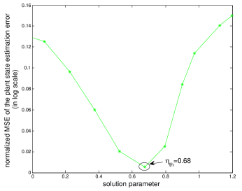
Figure 3: Normalized MSE of the plant state estimation versus $\eta_{th}$ at power cost 14dB.

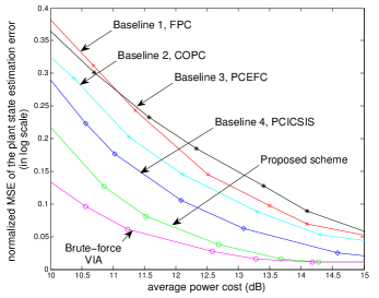
Figure 4: Normalized MSE of the plant state estimation average power cost.

Fig. 3 illustrates the normalized MSE of the plant state estimation versus $\eta_{th}$ at average power cost 14dB under our proposed scheme. The normalized MSE achieves the minimum when $\eta_{th}$ is around 0.68. Therefore, we choose $\eta_{th}=0.68$ when the average power cost is 14dB. The optimal choices of $\eta_{th}$ at other average power costs can be obtained using similar methods. Fig. 4 illustrates the normalized MSE of the plant state estimation versus the average power cost. Our proposed scheme achieves significant performance gain compared with all the baselines and the performance of the proposed scheme is very close to that of the brute-force VIA [12]. Table I illustrates the comparison of the computational time of the baselines, the proposed scheme, and the brute-force VIA [12]. Our proposed solution has very small computational cost due to the closed-form approximate value function in (LABEL:approxvaluefunc) and also outperforms the baselines.

Dimension of $\mathbf{x}$	2	4	6	8
BL 1 and 2	0.0034ms
BL 3	1.9s	3048.7s	$>10^{5}$s
BL 4	76.2s	$>10^{5}$s
Proposed scheme	$0.0924$s	$0.1696$s	$0.3316$s	$0.6284$s
VIA	108.6s	$>10^{5}$s

TABLE I: Comparison of the MATLAB computational time of the baselines, the proposed scheme, and the brute-force VIA.

VI Conclusion

In this paper, we propose a low complexity power control scheme for the NCS by solving a weighted average state estimation error and communication power minimization problem. Using a continuous-time perturbation approach, we derive a closed-form approximate value function and a low complexity power control scheme. The proposed solution is shown to have an event-driven structure with a dynamically changing threshold. We establish the conditions for asymptotic optimality, and also give sufficient conditions for ensuring the NCS stability under our proposed scheme. Numerical results show that the proposed scheme has low complexity and much better performance compared with the baselines.

Appendix A: Proof of Lemma 1

A. Analysis of the Primitive Quantizer

Following [3] and [5], we define the following constant matrices. Let $\boldsymbol{\Phi}$ be a nonsingular matrix and $\boldsymbol{\Upsilon}\in\mathbb{R}^{d\times d}$ such that $\boldsymbol{\Phi}\mathbf{F}\boldsymbol{\Phi}^{-1}=\boldsymbol{\Upsilon}=\text{diag}(\mathbf{J}_{1},\dots,\mathbf{J}_{m})$, where each $\mathbf{J}_{j}$ is a Jordan block of dimension $d_{j}$ (and $d_{j}$ is the geometric multiplicity associated with the eigenvalue $\lambda_{j}$). Define $\mathbf{H}=\text{diag}(\mathbf{H}_{1},\dots,\mathbf{H}_{m})$ and $\boldsymbol{\Gamma}=\text{diag}(\boldsymbol{\Gamma}_{1},\dots,\boldsymbol{\Gamma}_{m})$, where $\mathbf{H}_{j}=\mathbf{I}$ if $\mathbf{J}_{j}$ and $\boldsymbol{\Gamma}_{j}=\Bigg{(}\begin{smallmatrix}|\lambda_{j}|&1,&&\\ &|\lambda_{j}|&1&\\ &&\ddots&1\\ &&&|\lambda_{j}|\end{smallmatrix}\Bigg{)}$ if they are associated with real eigenvalue $\lambda_{j}$, and $\mathbf{H}_{j}=\text{diag}(r(\theta)^{-1},\dots,r(\theta)^{-1})$ with $r(\theta)=\Big{(}\begin{array}[]{cc}\cos(\theta),\ \sin(\theta)\\ -\sin(\theta),\cos(\theta)\end{array}\Big{)}$ and $\boldsymbol{\Gamma}_{j}=\Bigg{(}\begin{smallmatrix}|\lambda_{j}|&1,&&\\ &|\lambda_{j}|&1&\\ &&\ddots&1\\ &&&|\lambda_{j}|\end{smallmatrix}\Bigg{)}$ if $\mathbf{J}_{j}$ if they are associated with complex eigenvalues $\rho(\cos(\theta)\pm\sin(\theta))$. Define $\mathbf{F}_{\mathbf{R}}=\text{diag}(2^{-R_{1}},\dots,2^{-R_{d}})$. We summarize the working flow of the primitive quantizer as follows:

Algorithm 1 (Dynamic Update of the Primitive Quantizer).

At each time slot $t$, the primitive quantizer takes the plant state $\mathbf{x}(t)$ as input and does the following:

• Step 1, Initialization: If $t=0$, initialize the quantizer as follows: $\widetilde{\mathbf{x}}(0)=\mathbf{0}$, $\boldsymbol{\Psi}(0)=\boldsymbol{\Phi}$, $\mathbf{L}(0)=\|\boldsymbol{\Phi}\|L$, and go to Step 4. Otherwise, go to Step 2.

• Step 2, Update of the Shifting Vector and Data Pre-Processing:

  $$\widetilde{\mathbf{x}}(t)=\left\{\begin{aligned} &\mathbf{F}\widetilde{\mathbf{x}}(t-1)+\mathbf{G}\mathbf{u}(t-1),\ \text{if }\gamma(t-1)=0\\ &\mathbf{F}\left(\boldsymbol{\Psi}^{-1}(t-1)\boldsymbol{\xi}(t-1)+\widetilde{\mathbf{x}}(t-1)\right)\\ &\hskip 28.45274pt+\mathbf{G}\mathbf{u}(t-1),\ \text{if }\gamma(t-1)=1\end{aligned}\right.$$ (28)

  and $\widetilde{\mathbf{x}}(0)=\mathbf{x}_{0}$. Calculate innovation $\mathbf{i}(t)=\mathbf{x}(t)-\widetilde{\mathbf{x}}(t)$.

• Step 3, Update of the Coordinate Transformation Matrix and Dynamic Range:

  $$\boldsymbol{\Psi}(t)=\mathbf{H}\boldsymbol{\Psi}(t-1)$$ (29)

  $$\mathbf{L}(t)=\left\{\begin{aligned} &\boldsymbol{\Gamma}\mathbf{L}(t-1)+w_{max}\|\boldsymbol{\Psi}(t)\|\mathbf{1},\quad\text{if }\gamma(t-1)=0\\ &\boldsymbol{\Gamma}\mathbf{F}_{\mathbf{R}}\mathbf{L}(t-1)+w_{max}\|\boldsymbol{\Psi}(t)\|\mathbf{1},\text{if }\gamma(t-1)=1\end{aligned}\right.$$ (30)

  where $w_{max}=\widetilde{w}_{max}\sqrt{\int_{0}^{\tau}\int_{0}^{\tau}\mu_{max}\big{(}\exp(\widetilde{\mathbf{F}}^{T}s+\widetilde{\mathbf{F}}^{T}s^{\prime})\big{)}dsds^{\prime}}\\ =\mathcal{O}(\tau)$and $\|\mathbf{w}(t)\|\leq w_{max}$ according to (1).

• Step 4, Determination of the Output Symbol: The quantizer partitions the following region into $2^{2R}$ boxes:

  $$\mathcal{D}_{\widetilde{\mathbf{x}}}(t)=\big{\{}\mathbf{x}\in\mathbb{R}^{d}:\boldsymbol{\Psi}(t)\big{(}\mathbf{x}-\widetilde{\mathbf{x}}(t)\big{)}$$

  $$\in\left\{[-L_{1}(t),L_{1}(t)]\times\cdots\times[-L_{d}(t),L_{d}(t)]\right\}\big{\}}$$ (31)

  with side lengths $\big{\{}\frac{2L_{n}(t)}{2^{R_{n}}}:\forall n\big{\}}$. Determine which box $\mathbf{i}(t)$ falls into within the region $\mathcal{D}_{\widetilde{\mathbf{x}}}(t)$, and the quantizer outputs $\boldsymbol{\xi}(t)$, which is the centroid of that box. If $\mathbf{i}(t)$ falls outside the region $\mathcal{D}_{\widetilde{\mathbf{x}}}(t)$, the quantizer outputs a special symbol representing an overflow.    ∎

B. Properties of the Primitive Quantizer in Algorithm 1

Based on Algorithm 1, we can write the relationship between $\mathbf{x}(t)$ and $\boldsymbol{\xi}(t)$ as follows:

$$\boldsymbol{\xi}(t)=\boldsymbol{\Psi}(t)\big{(}\mathbf{x}(t)-\widetilde{\mathbf{x}}(t)\big{)}+\mathbf{e}(t)$$ (32)

where $\mathbf{e}(t)$ is the quantization noise. From (1), we know that $\mathbf{x}(t)$ is symmetrically distributed about the origin. Together with Algorithm 1, the primitive quantizer behaves like a multi-dimensional uniform quantizer [32]. Therefore, the quantization noise $\mathbf{e}(t)$ has zero mean. We obtain the dynamics of $\hat{\mathbf{x}}(t)$ and $\widetilde{\mathbf{x}}(t)$ as follows to show that $\mathbf{x}(t)$ never leaves $\mathcal{D}_{\widetilde{\mathbf{x}}}(t)$.

1) Dynamics of $\hat{\mathbf{x}}(t)=\mathbb{E}\big{[}\mathbf{x}(t)\big{|}I_{C}(t)\big{]}$: If $\gamma(t)=0$,

$$\hat{\mathbf{x}}(t) \overset{(a)}{=}\mathbb{E}\big{[}\mathbf{x}(t)\big{|}\mathbf{u}(t-1),\mathbf{u}_{0}^{t-2},\alpha_{0}^{t},\gamma_{0}^{\nu(t-1)},\mathbf{y}_{0}^{\nu(t-1)}\big{]}$$

$$\overset{(b)}{=}\mathbb{E}\big{[}\mathbf{F}\mathbf{x}(t-1)+\mathbf{w}(t-1)\big{|}I_{C}(t-1)\big{]}+\mathbf{G}\mathbf{u}(t-1)$$

$$\overset{(c)}{=}\mathbf{F}\hat{\mathbf{x}}(t-1)+\mathbf{G}\mathbf{u}(t-1)$$ (33)

where $(a)$ is according to the definition of $I_{C}(t)$ in (7), (b) is because $\mathbf{u}(t-1)$ is a function of $I_{C}(t-1)$ and $\{\mathbf{x}(t-1),\mathbf{w}(t-1)\}$ is independent of $\alpha(t)$, and $(c)$ is because $\mathbb{E}\big{[}\mathbf{w}(t-1)\big{|}I_{C}(n-1)\big{]}=0$. If $\gamma(t)=1$,

$$\hat{\mathbf{x}}(t) \overset{(d)}{=}\mathbb{E}\big{[}\boldsymbol{\Psi}^{-1}(t)\big{(}\boldsymbol{\xi}(t)-\mathbf{e}(t)\big{)}+\widetilde{\mathbf{x}}(t)\big{|}$$

$$\hskip 28.45274pt\boldsymbol{\xi}(t),\widetilde{\mathbf{x}}(t),\mathbf{u}_{0}^{t-1},\alpha_{0}^{t},\gamma_{0}^{\nu(t-1)},\mathbf{y}_{0}^{\nu(t-1)}\big{]}$$

$$\overset{(e)}{=}\boldsymbol{\Psi}^{-1}(t)\boldsymbol{\xi}(t)+\widetilde{\mathbf{x}}(t)$$ (34)

where $(d)$ is due to the successful transmission of $\boldsymbol{\xi}(t)$ and $(e)$ is due to the zero mean quantization noise $\mathbf{e}(t)$ and the fact that $\widetilde{\mathbf{x}}(t)$ can be locally obtained at the controller.

Therefore,

$$\hat{\mathbf{x}}(t)=\left\{\begin{aligned} &\mathbf{F}\hat{\mathbf{x}}(t-1)+\mathbf{G}\mathbf{u}(t-1),\quad&\text{if }\gamma(t)=0\\ &\boldsymbol{\Psi}^{-1}(t)\boldsymbol{\xi}(t)+\widetilde{\mathbf{x}}(t),\quad&\text{if }\gamma(t)=1\end{aligned}\right.$$ (35)

where $\hat{\mathbf{x}}(0)=\mathbf{x}_{0}$ if $\gamma(0)=0$.

2) Dynamics of $\widetilde{\mathbf{x}}(t)=\mathbb{E}\big{[}\mathbf{x}(t)\big{|}I_{SC}(t)\big{]}$: If $\gamma(t-1)=0$,

$$\widetilde{\mathbf{x}}(t) =\mathbb{E}\big{[}\mathbf{F}\mathbf{x}(t-1)+\mathbf{w}(t-1)\big{|}I_{SC}(t-1)\big{]}+\mathbf{G}\mathbf{u}(t-1)$$

$$=\mathbf{F}\widetilde{\mathbf{x}}(t-1)+\mathbf{G}\mathbf{u}(t-1)$$ (36)

where (36) follows (b) and (c) in (33). If $\gamma(t-1)=1$,

$$\widetilde{\mathbf{x}}(t) =\mathbb{E}\big{[}\mathbf{F}\mathbf{x}(t-1)+\mathbf{w}(t-1)\big{|}\boldsymbol{\xi}(t-1),\widetilde{\mathbf{x}}(t-1),$$

$$\mathbf{u}_{0}^{t-1},\alpha_{0}^{t-1},\gamma_{0}^{\nu(t-2)},\mathbf{y}_{0}^{\nu(t-2)}\big{]}+\mathbf{G}\mathbf{u}(t-1)$$

$$=\mathbf{F}\big{(}\boldsymbol{\Psi}^{-1}(t-1)\boldsymbol{\xi}(t-1)+\widetilde{\mathbf{x}}(t)\big{)}+\mathbf{G}\mathbf{u}(t-1)$$ (37)

where (37) follows the calculations in (34).

3) Dynamic Range of $\mathbf{x}(t)$: We prove the following lemma:

Lemma 5.

At each time slot $t$, we have $\mathbf{x}(t)\in\mathcal{D}_{\widetilde{\mathbf{x}}}(t)$, where $\mathcal{D}_{\widetilde{\mathbf{x}}}(t)$ is given in (31).

  Proof: We define the following range:

$$\mathcal{E}_{\hat{\mathbf{x}}}(t)= \big{\{}\mathbf{x}\in\mathbb{R}^{d}:\boldsymbol{\Psi}(t)\big{(}\mathbf{x}-\hat{\mathbf{x}}(t)\big{)}$$ (38)

$$\in\left\{[-\Lambda_{1}(t),\Lambda_{1}(t)]\times\cdots\times[-\Lambda_{d}(t),\Lambda_{d}(t)]\right\}\big{\}}$$

where $\boldsymbol{\Lambda}(t)=\big{(}\Lambda_{1}(t),\dots,\Lambda_{d}(t)\big{)}^{T}\in\mathbb{R}^{d}$ with the following dynamics:

$$\boldsymbol{\Lambda}(t)=\left\{\begin{aligned} &\mathbf{F}_{\mathbf{R}}\mathbf{L}(t),\hskip 82.51282pt\text{if }\gamma(t)=1\\ &\mathbf{L}(t),\hskip 96.73918pt\text{if }\gamma(t)=0,\gamma(t-1)=1\\ &\boldsymbol{\Gamma}\boldsymbol{\Lambda}(t-1)+w_{max}\|\boldsymbol{\Psi}(t)\|\mathbf{1},\text{if }\gamma(t)=0,\gamma(t-1)=0\end{aligned}\right.$$

and we let $\gamma(-1)=1$.We will show in sequence: if $\mathbf{x}(t)\in\mathcal{D}_{\widetilde{\mathbf{x}}}(t)$, then $\mathbf{x}(t)\in\mathcal{E}_{\hat{\mathbf{x}}}(t)$, and if $\mathbf{x}(t)\in\mathcal{E}_{\hat{\mathbf{x}}}(t)$, then $\mathbf{x}(t+1)\in\mathcal{D}_{\widetilde{\mathbf{x}}}(t+1)$. Using induction method, the initial condition of the primitive quantizer in Algorithm 1 ensures that $\mathbf{x}(0)\in\mathcal{D}_{\widetilde{\mathbf{x}}}(0)$ (according to Prop. 5.1 of [3]), and then,
a. $\mathbf{x}(t)\in\mathcal{D}_{\widetilde{\mathbf{x}}}(t)\Rightarrow\mathbf{x}(t)\in\mathcal{E}_{\hat{\mathbf{x}}}(t)$:

• Case 1 ($\gamma(t)=1$): Using (32) and (LABEL:errordyn), we have $\boldsymbol{\Psi}(t)\ (\mathbf{x}(t)-\hat{\mathbf{x}}(t)\ )=-\mathbf{e}(t)$. If $\mathbf{x}(t)\in\mathcal{D}_{\widetilde{\mathbf{x}}}(t)$, we have $|e_{n}(t)|\leq\frac{L_{n}(t)}{2^{-R_{n}}}$ for all $n$. Therefore, we have $\mathbf{x}(t)\in\mathcal{E}_{\hat{\mathbf{x}}}(t)$ with $\boldsymbol{\Lambda}(t)=\mathbf{F}_{\mathbf{R}}\mathbf{L}(t)$.

• Case 2 ($\gamma(t)=0$, $\gamma(t-1)=1$): Using (LABEL:errordynfake) and (LABEL:errordyn), we have $\boldsymbol{\Psi}(t)\ (\mathbf{x}(t)-\hat{\mathbf{x}}(t)\ )=\boldsymbol{\Psi}(t)\ (\mathbf{x}(t)-\widetilde{\mathbf{x}}(t)\ )$. Therefore, if $\mathbf{x}(t)\in\mathcal{D}_{\widetilde{\mathbf{x}}}(t)$, then $\mathbf{x}(t)\in\mathcal{E}_{\hat{\mathbf{x}}}(t)$ with $\boldsymbol{\Lambda}(t)=\mathbf{L}(t)$.

• Case 3 ($\gamma(t)=0$, $\gamma(t-1)=0$): Using (1) and (LABEL:errordyn), we have $\boldsymbol{\Psi}(t)\ (\mathbf{x}(t)-\hat{\mathbf{x}}(t)\ )=\boldsymbol{\Psi}(t)\ (\mathbf{F}\ (\mathbf{x}(t-1)-\hat{\mathbf{x}}(t-1)\ )+\mathbf{w}(t-1)\ )=\mathbf{H}\mathbf{\Upsilon}\ (\boldsymbol{\Psi}(t-1)\ (\mathbf{x}(t-1)-\hat{\mathbf{x}}(t-1)\ )\ )+\boldsymbol{\Psi}(t)\mathbf{w}(t-1)$, where the second equality is due to Lemma 4.1 of [3]. If $\mathbf{x}(t)\in\mathcal{D}_{\widetilde{\mathbf{x}}}(t)$, using Lemma 4.2 of [3], then $\mathbf{x}(t)\in\mathcal{E}_{\hat{\mathbf{x}}}(t)$ with $\boldsymbol{\Lambda}(t)=\boldsymbol{\Gamma}\boldsymbol{\Lambda}(t-1)+w_{max}\|\boldsymbol{\Psi}(t)\|\mathbf{1}$.

b. $\mathbf{x}(t)\in\mathcal{E}_{\hat{\mathbf{x}}}(t)\Rightarrow\mathbf{x}(t+1)\in\mathcal{D}_{\widetilde{\mathbf{x}}}(t+1)$:

• Case 1 ($\gamma(t)=1$): Using (1), (LABEL:errordynfake), (LABEL:errordyn) and Lemma 4.1 of [3], we have $\boldsymbol{\Psi}(t+1)(\mathbf{x}(t+1)-\widetilde{\mathbf{x}}(t+1))=\mathbf{H}\mathbf{\Upsilon}(\boldsymbol{\Psi}(t)(\mathbf{x}(t)-\hat{\mathbf{x}}(t)))+\boldsymbol{\Psi}(t+1)\mathbf{w}(t)$. If $\mathbf{x}(t)\in\mathcal{E}_{\hat{\mathbf{x}}}(t)$, using Lemma 4.2 of [3], then $\mathbf{x}(t+1)\in\mathcal{D}_{\widetilde{\mathbf{x}}}(t+1)$ with $\mathbf{L}(t+1)=\boldsymbol{\Gamma}\boldsymbol{\Lambda}(t)+w_{max}\|\boldsymbol{\Psi}(t+1)\|\mathbf{1}=\boldsymbol{\Gamma}\mathbf{F}_{\mathbf{R}}\mathbf{L}(t)+w_{max}\|\boldsymbol{\Psi}(t+1)\|\mathbf{1}$. This is the evolution of $\mathbf{L}(t)$ for successful transmission in (30).

• Case 2 ($\gamma(t)=0$): Using (1), (LABEL:errordynfake) and Lemma 4.1 of [3], we have $\boldsymbol{\Psi}(t+1)(\mathbf{x}(t+1)-\widetilde{\mathbf{x}}(t+1))=\mathbf{H}\mathbf{\Upsilon}(\boldsymbol{\Psi}(t)(\mathbf{x}(t)-\widetilde{\mathbf{x}}(t)))+\boldsymbol{\Psi}(t+1)\mathbf{w}(t)$. If $\mathbf{x}(t)\in\mathcal{E}_{\hat{\mathbf{x}}}(t)$, using Lemma 4.2 of [3], and then $\mathbf{x}(t+1)\in\mathcal{D}_{\widetilde{\mathbf{x}}}(t+1)$ with $\mathbf{L}(t+1)=\boldsymbol{\Gamma}\boldsymbol{\Lambda}(t)+w_{max}\|\boldsymbol{\Psi}(t+1)\|\mathbf{1}=\boldsymbol{\Gamma}\mathbf{L}(t)+w_{max}\|\boldsymbol{\Psi}(t+1)\|\mathbf{1}$. This is the evolution of $\mathbf{L}(t)$ for unsuccessful transmission in (30).   ∎

Lemma 5 proves the first property in Lemma 1. Together with the results in Section 5.1.4 of [32] on the uniform quantizer , the quantization noise $\mathbf{e}(t)=\big{(}e_{1}(t),\dots,e_{d}(t)\big{)}^{T}$ has a uniform distribution, where $e_{n}(t)$ is uniformly distributed within the region $\big{[}-\frac{L_{n}(t)}{2^{R_{n}-1}},\frac{L_{n}(t)}{2^{R_{n}-1}}\big{]}$. This proves the second property in Lemma 1 (where we use $\mathbf{e}(\mathbf{L}(t),t)$ to denote the quantization noise to show its dependence on $\mathbf{L}(t)$).

Appendix B: Proof of Lemma 2

A. Relationship between the Original NCS and an Autonomous NCS

We consider two NCSs. The first NCS is given as follows:

$$\mathbf{x}(t+1)=\mathbf{F}\mathbf{x}(t)+\mathbf{G}\mathbf{u}(t)+\mathbf{w}(t)$$

$$\boldsymbol{\xi}(t)=Q_{\boldsymbol{\Psi}(t),\mathbf{L}(t)}\big{(}\mathbf{x}(t)-\widetilde{\mathbf{x}}(t)\big{)},\quad\mathbf{y}(t)=\gamma(t)\boldsymbol{\xi}(t)$$ (39)

where $Q_{\boldsymbol{\Psi}(t),\mathbf{L}(t)}(\cdot)$ corresponds to the R.H.S. of the mapper model in (9). The second NCS is given as follows with no control actions applied (i.e., an autonomous system):

$$\overline{\mathbf{x}}(t+1)=\mathbf{F}\overline{\mathbf{x}}(t)+\overline{\mathbf{w}}(t)$$

$$\overline{\boldsymbol{\xi}}(t)=Q_{\overline{\boldsymbol{\Psi}}(t),\overline{\mathbf{L}}(t)}\big{(}\overline{\mathbf{x}}(t)-\widetilde{\overline{\mathbf{x}}}(t)\big{)},\quad\overline{\mathbf{y}}(t)=\overline{\gamma}(t)\overline{\boldsymbol{\xi}}(t)$$ (40)

where $\widetilde{\overline{\mathbf{x}}}(t)=\mathbb{E}\big{[}\mathbf{x}(t)\big{|}\overline{I}_{SC}(t)\big{]}$ and $\overline{I}_{SC}(t)\triangleq\{\overline{\alpha}_{0}^{t-1},\overline{\gamma}_{0}^{\nu(t-1)},\overline{\mathbf{y}}_{0}^{\nu(t-1)}\}$, and we assume the following parameters are identical in the two NCSs, i.e., $\mathbf{x}(0)=\overline{\mathbf{x}}(0)$, $\mathbf{w}(t)=\overline{\mathbf{w}}(t)$, $\boldsymbol{\Psi}(t)=\overline{\boldsymbol{\Psi}}(t)$, $\mathbf{L}(t)=\overline{\mathbf{L}}(t)$, $\alpha(t)=\overline{\alpha}(t)$, $\gamma(t)=\overline{\gamma}(t)$, for all $t$. Then,

Lemma 6.

For the two NCSs in (39) and (40), we have $\mathbf{x}(t)-\mathbb{E}\big{[}\mathbf{x}(t)|I_{C}(t)\big{]}=\overline{\mathbf{x}}(t)-\mathbb{E}\big{[}\overline{\mathbf{x}}(t)|I_{C}(t)\big{]}$, $\forall t$.

Proof.

The linearity of the dynamics for $\mathbf{x}(t)$ and $\overline{\mathbf{x}}(t)$ implies the existence of $\mathbf{A}(t)$, $\mathbf{B}(t)$ and $\mathbf{C}(t)$ such that

$$\mathbf{x}(t)=\mathbf{A}(t)\mathbf{x}(0)+\mathbf{B}(t)\vec{\mathbf{u}}(t-1)+\mathbf{C}(t)\vec{\mathbf{w}}(t-1)$$

$$\overline{\mathbf{x}}(t)=\mathbf{A}(t)\mathbf{x}(0)+\mathbf{C}(t)\vec{\mathbf{w}}(t-1)$$ (41)

where $\vec{\mathbf{u}}(t)=(\mathbf{u}^{T}(1),\dots,\mathbf{u}(t))^{T}$ and $\vec{\mathbf{w}}(t)=(\mathbf{w}^{T}(1),\dots,\mathbf{w}(t))^{T}$. Then, we have $\mathbf{x}(t)-\mathbb{E}\big{[}\mathbf{x}(t)|I_{C}(t)\big{]}=\big{(}\mathbf{A}(t)\mathbf{x}(0)+\mathbf{C}(t)\vec{\mathbf{w}}(t-1)\big{)}\-\big{(}\mathbf{A}(t)\mathbb{E}\big{[}\mathbf{x}(0)|I_{C}(t)\big{]}+\mathbf{C}(t)\mathbb{E}\big{[}\vec{\mathbf{w}}(t-1)|I_{C}(t)\big{]}\big{)}=\overline{\mathbf{x}}(t)-\mathbb{E}\big{[}\overline{\mathbf{x}}(t)|I_{C}(t)\big{]}$.∎

B. State Estimate of an Autonomous System

We then prove the following Lemma. Together with Lemma 6, the no dual effect property of the original NCS can be directly proven.

Lemma 7.

$\mathbb{E}\big{[}\overline{\mathbf{x}}(t)|I_{C}(t)\big{]}=\mathbb{E}\big{[}\overline{\mathbf{x}}(t)|\alpha_{0}^{t},\gamma_{0}^{\nu(t)},\overline{\mathbf{y}}_{0}^{\nu(t)}\big{]}$, $\forall t$.

Proof.

We use $X\rightarrow Y\rightarrow Z$ to denote that $(X,Y,Z)$ forms a Markov chain, i.e., $\Pr[Z|X,Y]=\Pr[Z|Y]$. It can be easily verified that $X\rightarrow Y\rightarrow Z$ implies that $Z\rightarrow Y\rightarrow X$. Using induction method, we will show that $\overline{\mathbf{y}}(\nu(t))=\mathbf{y}(\nu(t))$ and $\overline{\mathbf{x}}(t)\rightarrow\{\alpha_{0}^{t},\gamma_{0}^{\nu(t)},\mathbf{y}_{0}^{\nu(t)}\}\rightarrow\mathbf{u}_{0}^{t-1}$ for all $t\geq 1$.

Step 1 ($t=1$): If $\gamma(0)=0$, we have $\overline{\mathbf{y}}(\nu(0))=\mathbf{y}(\nu(0))=0$. If $\gamma(0)=1$, we have $\overline{\mathbf{y}}(\nu(0))=Q_{\overline{\boldsymbol{\Psi}}(0),\overline{\mathbf{L}}(0)}\big{(}\overline{\mathbf{x}}(0)-\widetilde{\overline{\mathbf{x}}}(0)\big{)}=Q_{{\boldsymbol{\Psi}}(0),{\mathbf{L}}(0)}\big{(}{\mathbf{x}}(0)-\widetilde{{\mathbf{x}}}(0)\big{)}={\mathbf{y}}(\nu(0))$, where the second equality is due to the construction in part A. Therefore, $\overline{\mathbf{y}}(\nu(0))=\mathbf{y}(\nu(0))$. Since $\mathbf{u}(0)=\sigma(I_{C}(0))=\sigma(\{\alpha_{0},\gamma_{0}^{\nu(0)},\mathbf{y}_{0}^{\nu(0)}\})$, we have $\{\overline{\mathbf{x}}_{0},\mathbf{w}(0)\}\rightarrow\{\alpha_{0},\gamma_{0}^{\nu(0)},\mathbf{y}_{0}^{\nu(0)}\}\rightarrow\mathbf{u}(0)$. Together with $\overline{\mathbf{x}}(1)=\mathbf{F}\overline{\mathbf{x}}(0)+\overline{\mathbf{w}}(0)$, we have

$$\overline{\mathbf{x}}(1)\rightarrow\{\alpha_{0}^{1},\gamma_{0}^{\nu(0)},\mathbf{y}_{0}^{\nu(0)}\}\rightarrow\mathbf{u}(0)$$ (42)

Therefore, we have $\overline{\mathbf{y}}(\nu(1))=\overline{\mathbf{y}}(\nu(0))=\mathbf{y}(\nu(0))=\mathbf{y}(\nu(1))$ if $\gamma(1)=0$. If $\gamma(1)=1$, we have

$$\overline{\mathbf{y}}(\nu(1))=\overline{\mathbf{y}}(1)=Q_{\boldsymbol{\Psi}(1),{\mathbf{L}}(1)}\big{(}\overline{\mathbf{x}}(1)-\mathbb{E}\big{[}\overline{\mathbf{x}}(1)\big{|}{\alpha}_{0}^{1},{\gamma}_{0}^{\nu(0)},\mathbf{y}_{0}^{\nu(0)}\big{]}\big{)}$$

$$\overset{(a)}{=} Q_{\boldsymbol{\Psi}(1),{\mathbf{L}}(1)}\big{(}\overline{\mathbf{x}}(1)-\mathbb{E}\big{[}\overline{\mathbf{x}}(1)\big{|}I_{SC}(1)\big{]}\big{)}$$ (43)

$$\overset{(b)}{=} Q_{\boldsymbol{\Psi}(1),{\mathbf{L}}(1)}\big{(}{\mathbf{x}}(1)-\mathbb{E}\big{[}{\mathbf{x}}(1)\big{|}I_{SC}(1)\big{]}\big{)}=\mathbf{y}(1)=\mathbf{y}(\nu(1))$$

where (a) is due to (42), and (b) can be verified similarly as in Lemma 6. Therefore, $\overline{\mathbf{y}}(\nu(1))={\mathbf{y}}(\nu(1))$. Furthermore, since $\overline{\mathbf{y}}(\nu(1))={\mathbf{y}}(\nu(1))=\sigma\big{(}\alpha_{0}^{1},\gamma_{0}^{\nu(1)},\mathbf{y}_{0}^{\nu(0)},\overline{\mathbf{x}}(1)\big{)}$, we have

$$\Pr[\mathbf{u}(0)|\alpha_{0}^{1},\gamma_{0}^{\nu(1)},\mathbf{y}_{0}^{\nu(1)},\overline{\mathbf{x}}(1)]$$

$$= \Pr[\mathbf{u}(0)|\alpha_{0}^{1},\gamma_{0}^{\nu(1)},\mathbf{y}_{0}^{\nu(0)},\sigma\big{(}\alpha_{0}^{1},\gamma_{0}^{\nu(1)},\mathbf{y}_{0}^{\nu(0)},\overline{\mathbf{x}}(1)\big{)},\overline{\mathbf{x}}(1)]$$

$$\overset{(c)}{=} \Pr[\mathbf{u}(0)|\alpha_{0}^{1},\gamma_{0}^{\nu(1)},\mathbf{y}_{0}^{\nu(0)},\sigma\big{(}\alpha_{0}^{1},\gamma_{0}^{\nu(1)},\mathbf{y}_{0}^{\nu(0)}\big{)}]$$ (44)

where $(c)$ is due to (42). Therefore, based on (44), we have $\overline{\mathbf{x}}(1)\rightarrow\{\alpha_{0}^{1},\gamma_{0}^{\nu(1)},\mathbf{y}_{0}^{\nu(1)}\}\rightarrow\mathbf{u}(0)$.

Step 2 (Induction): By induction hypothesis, assume that $\overline{\mathbf{y}}(\nu(t))=\mathbf{y}(\nu(t))$ and for $1\leq k\leq t$. Note that $\{\overline{\mathbf{x}}(t),\mathbf{w}(t)\}\rightarrow\{\mathbf{u}_{0}^{t-1},\alpha_{0}^{t},\gamma_{0}^{\nu(t)},\mathbf{y}_{0}^{\nu(t)}\}\rightarrow\mathbf{u}(t)$ because $\mathbf{u}(t)$ only depends on $I_{C}(t)$. By the induction hypothesis and $\mathbf{w}(t)$ is independent of $\mathbf{y}_{0}^{\nu(t)}$ and $\mathbf{u}_{0}^{t-1}$, we have $\{\overline{\mathbf{x}}(t),\mathbf{w}(t)\}\rightarrow\{\alpha_{0}^{t},\gamma_{0}^{\nu(t)},\mathbf{y}_{0}^{\nu(t)}\}\rightarrow\mathbf{u}_{0}^{t-1}$. Combining the above results, we have $\{\overline{\mathbf{x}}(t),\mathbf{w}(t)\}\rightarrow\{\alpha_{0}^{t},\gamma_{0}^{\nu(t)},y_{0}^{\nu(t)}\}\rightarrow\mathbf{u}_{0}^{t}$. Together with $\overline{\mathbf{x}}(t+1)=\mathbf{F}\overline{\mathbf{x}}(t)+\overline{\mathbf{w}}(t)$, we have

$$\overline{\mathbf{x}}(t+1)\rightarrow\{\alpha_{0}^{t+1},\gamma_{0}^{\nu(t)},\mathbf{y}_{0}^{\nu(t)}\}\rightarrow\mathbf{u}_{0}^{t}$$ (45)

Therefore, we have $\overline{\mathbf{y}}(\nu(t+1))=\overline{\mathbf{y}}(\nu(t))=\mathbf{y}(\nu(t))=\mathbf{y}(\nu(t+1))$ if $\gamma(t+1)=0$. If $\gamma(t+1)=1$, following the same derivations in (43) and using (45), we have $\overline{\mathbf{y}}(\nu(t+1))=\overline{\mathbf{y}}(t+1)=Q_{\boldsymbol{\Psi}(t+1),{\mathbf{L}}(t+1)}\big{(}\overline{\mathbf{x}}(t+1)-\mathbb{E}\big{[}\overline{\mathbf{x}}(t+1)\big{|}I_{SC}(t+1)\big{]}\big{)}=Q_{\boldsymbol{\Psi}(t+1),{\mathbf{L}}(t+1)}\big{(}{\mathbf{x}}(t+1)-\mathbb{E}\big{[}{\mathbf{x}}(t+1)\big{|}I_{SC}(t+1)\big{]}\big{)}=\mathbf{y}(\nu(t+1))$. Therefore, $\overline{\mathbf{y}}(\nu(t+1))={\mathbf{y}}(\nu(t+1))$. Furthermore, since $\overline{\mathbf{y}}(\nu(t+1))={\mathbf{y}}(\nu(t+1))=\sigma\big{(}\alpha_{0}^{t+1},\gamma_{0}^{\nu(t+1)},\mathbf{y}_{0}^{\nu(t)},\overline{\mathbf{x}}(t+1)\big{)}$, we have

$$\Pr[\mathbf{u}_{0}^{t}|\alpha_{0}^{t+1},\gamma_{0}^{\nu(t+1)},\mathbf{y}_{0}^{\nu(t+1)},\overline{\mathbf{x}}(t+1)]$$

$$= \Pr[\mathbf{u}_{0}^{t}|\alpha_{0}^{t+1},\gamma_{0}^{\nu(t+1)},\mathbf{y}_{0}^{\nu(t)},$$

$$\sigma\big{(}\alpha_{0}^{t+1},\gamma_{0}^{\nu(t+1)},\mathbf{y}_{0}^{\nu(t)},\overline{\mathbf{x}}(t+1)\big{)},\overline{\mathbf{x}}(t+1)]$$

$$\overset{(d)}{=} \Pr[\mathbf{u}_{0}^{t}|\alpha_{0}^{t+1},\gamma_{0}^{\nu(t+1)},\mathbf{y}_{0}^{\nu(t)},\sigma\big{(}\alpha_{0}^{t+1},\gamma_{0}^{\nu(t+1)},\mathbf{y}_{0}^{\nu(t)}\big{)}]$$ (46)

where $(d)$ is due to (45). Therefore, based on (46), we have $\overline{\mathbf{x}}(t+1)\rightarrow\{\alpha_{0}^{t+1},\gamma_{0}^{\nu(t+1)},\mathbf{y}_{0}^{\nu(t+1)}\}\rightarrow\mathbf{u}_{0}^{t}$.∎

Finally, combining Lemma 6 and Lemma 7, we have

$$\boldsymbol{\Delta}(t)=\mathbf{x}(t)-\mathbb{E}\big{[}\mathbf{x}(t)|I_{C}(t)\big{]}=\overline{\mathbf{x}}(t)-\mathbb{E}\big{[}\overline{\mathbf{x}}(t)|\alpha_{0}^{t},\gamma_{0}^{\nu(t)},\overline{\mathbf{y}}_{0}^{\nu(t)}\big{]}$$

Therefore, $\boldsymbol{\Delta}(t)$ does not dependent on $\mathbf{u}_{0}^{t-1}$, which directly induces the no dual effect property in Lemma 2.

Appendix C: Proof of Theorem 1

For a given $\Omega_{p}$, the induced process $\mathbf{Y}(t)=\big{\{}\mathbf{x}_{0}^{t},\mathbf{i}_{0}^{t},\mathbf{u}_{0}^{t-1},\boldsymbol{\xi}_{0}^{t},\alpha_{0}^{t-1},\gamma_{0}^{t-1},\boldsymbol{\Psi}_{0}^{t},\mathbf{L}_{0}^{t}\big{\}}\in\sigma\big{(}\big{\{}I_{S}(s):0\leq s\leq t\big{\}}\big{)}$is a controlled Markov process with transition kernel:

$$\Pr\big{[}\mathbf{Y}(t+1)\big{|}\mathbf{Y}(t),p(t)\big{]}=\Pr\big{[}\mathbf{x}(t+1)\big{|}\mathbf{x}(t),\mathbf{u}(t)\big{]}$$

$$\cdot\Pr\big{[}\mathbf{u}(t)\big{|}\gamma(t),\mathbf{Y}(t)\big{]}\Pr\big{[}\gamma(t)\big{|}\alpha(t),p(t)\big{]}\Pr\big{[}\alpha(t)\big{|}\alpha(t-1)\big{]}$$

$$\cdot\Pr\big{[}\boldsymbol{\xi}(t+1)\big{|}\mathbf{i}(t+1),\boldsymbol{\Psi}(t+1),\mathbf{L}(t+1)\big{]}$$

$$\cdot\Pr\big{[}\mathbf{i}(t+1)\big{|}\boldsymbol{\Psi}(t),\boldsymbol{\xi}(t),\gamma(t),\mathbf{i}(t)\big{]}$$

$$\cdot\Pr\big{[}\boldsymbol{\Psi}(t+1)\big{|}\boldsymbol{\Psi}(t)\big{]}\Pr\big{[}\mathbf{L}(t+1)\big{|}\mathbf{L}(t),\gamma(t)\big{]}$$ (47)

where each term can be calculated using the associated state dynamics in (1), (LABEL:errordyn), (4), (2), (32), (LABEL:errordynfake), (29), and (30).

Note that the dynamics of $\boldsymbol{\Delta}(t)$ in (13) can be obtained from the dynamics of $\mathbf{x}(t)$ and $\hat{\mathbf{x}}(t)$ in (1) and (LABEL:errordyn). Based on $\boldsymbol{\Delta}(t)$ in (13), the per-stage cost of the MDP is reduced to

$$\mathbb{E}[\big{(}\boldsymbol{\Delta}^{T}(t)\mathbf{S}\boldsymbol{\Delta}(t)+\lambda p\big{)}\tau|\mathbf{Y}(t)]=\mathbb{E}[\big{(}\boldsymbol{\Delta}^{T}(t)\mathbf{S}\boldsymbol{\Delta}(t)+\lambda p\big{)}\tau|\boldsymbol{\chi}(t)]$$

where $\boldsymbol{\chi}(t)\triangleq\big{\{}\boldsymbol{\Delta}(t-1),\alpha(t-1),\boldsymbol{\Psi}(t),\mathbf{L}(t)\big{\}}\subset\mathbf{Y}(t)$ with the associated transition kernel given by

$$\Pr\big{[}\boldsymbol{\chi}(t+1)\big{|}\boldsymbol{\chi}(t),p(t)\big{]}=\Pr\big{[}\alpha(t)\big{|}\alpha(t-1)\big{]}$$

$$\cdot\Pr\big{[}\boldsymbol{\Psi}(t+1)\big{|}\boldsymbol{\Psi}(t)\big{]}\Pr\big{[}\mathbf{L}(t+1)\big{|}\mathbf{L}(t),\alpha(t),p(t)\big{]}$$

$$\cdot\Pr\big{[}\boldsymbol{\Delta}(t)\big{|}\boldsymbol{\Delta}(t-1),\boldsymbol{\Psi}(t),\mathbf{L}(t),\alpha(t),p(t)\big{]}$$

where $\Pr\big{[}\boldsymbol{\Delta}(t)\big{|}\boldsymbol{\Delta}(t-1),\boldsymbol{\Psi}(t),\mathbf{L}(t),\alpha(t),p(t)\big{]}$ is associated with the dynamics of $\boldsymbol{\Delta}(t)$ in (13). Hence, Problem 1 is an MDP with system state being $\boldsymbol{\chi}$, and the optimality condition in Theorem 1 directly follows from Prop. 4.6.1 of [12].

Appendix D: Proof of Lemma 3

For convenience, denote

$$T_{\boldsymbol{\chi}}(\theta,V,p)=\frac{1}{\tau}\mathbb{E}\big{[}\big{(}(\boldsymbol{\Delta}^{\prime})^{T}\mathbf{S}(\boldsymbol{\Delta}^{\prime})+\lambda p\big{)}\tau$$ (48)

$$\qquad+\sum_{\boldsymbol{\chi}^{\prime}}\Pr\left[\boldsymbol{\chi}^{\prime}\big{|}\boldsymbol{\chi},p\right]V\left(\boldsymbol{\chi}^{\prime}\right)-V\left(\boldsymbol{\chi}\right)\big{|}\boldsymbol{\chi}\big{]}-\theta$$

$$T_{\boldsymbol{\chi}}^{\dagger}(\theta,V,p)=\boldsymbol{\Delta}^{T}\mathbf{S}\boldsymbol{\Delta}+\big{[}\lambda+\big{(}V(\mathbf{0},\alpha,\boldsymbol{\Psi},\mathbf{L})$$ (49)

$$-V(\boldsymbol{\Delta},\alpha,\boldsymbol{\Psi},\mathbf{L})\big{)}\frac{\alpha}{\kappa(R)B_{W}}\big{]}p+\nabla_{\boldsymbol{\Delta}}^{T}V(\boldsymbol{\Delta},\alpha,\boldsymbol{\Psi},\mathbf{L})\widetilde{\mathbf{F}}\boldsymbol{\Delta}$$

$$+\frac{1}{2}\text{Tr}\big{(}\nabla_{\boldsymbol{\Delta}}^{2}V(\boldsymbol{\Delta},\alpha,\boldsymbol{\Psi},\mathbf{L})\widetilde{\mathbf{W}}\big{)}+\frac{\partial V(\boldsymbol{\Delta},\alpha,\boldsymbol{\Psi},\mathbf{L})}{\partial\alpha}\left(2\widetilde{a}\alpha+2\widetilde{a}\right)$$

$$+\frac{\partial^{2}V^{\ast}(\boldsymbol{\Delta},\alpha,\boldsymbol{\Psi},\mathbf{L})}{\partial\alpha^{2}}4\widetilde{a}\alpha+\text{Tr}\big{(}\frac{\partial V(\boldsymbol{\Delta},\alpha,\boldsymbol{\Psi},\mathbf{L})}{\partial\boldsymbol{\Psi}}(\mathbf{H}\boldsymbol{\Psi}-\boldsymbol{\Psi})/\tau\big{)}$$

$$+\nabla^{T}_{\mathbf{L}}V(\boldsymbol{\Delta},\alpha,\boldsymbol{\Psi},\mathbf{L})\big{(}\boldsymbol{\Gamma}\mathbf{F}_{\mathbf{R}}\mathbf{L}+w_{max}\|\mathbf{H}\boldsymbol{\Psi}\|\mathbf{1}-\mathbf{L}\big{)}/\tau-\theta$$

A. Relationship between $T_{\boldsymbol{\chi}}(\theta,V,p)$ and $T_{\boldsymbol{\chi}}^{\dagger}(\theta,V,p)$

Lemma 8.

For any $\boldsymbol{\chi}$, $T_{\boldsymbol{\chi}}(\theta,V,p)=T_{\boldsymbol{\chi}}^{\dagger}(\theta,V,p)+\mathcal{O}(\tau)+\mathcal{O}\big{(}\frac{\tau^{2}}{2^{2R_{min}}}\big{)}$.

Proof of Lemma 8.

a. Calculation of the per-stage cost: We first calculate the per-stage cost in (14):

$$\mathbb{E}\big{[}(\boldsymbol{\Delta}^{\prime})^{T}\mathbf{S}(\boldsymbol{\Delta}^{\prime})\tau\big{|}\boldsymbol{\chi}\big{]}$$ (50)

$$= \mathbb{E}\big{[}\mathbf{e}^{T}(\mathbf{L})\boldsymbol{\Psi}^{-T}\boldsymbol{\Psi}^{-1}\mathbf{e}(\mathbf{L})\tau\Pr\left[\gamma(t)=1\right]$$

$$+\left(\mathbf{F}\boldsymbol{\Delta}+\mathbf{w}\right)^{T}\mathbf{S}\left(\mathbf{F}\boldsymbol{\Delta}+\mathbf{w}\right)\tau\Pr\left[\gamma(t)=0\right]\big{|}\boldsymbol{\chi}\big{]}$$

$$\overset{(a)}{=} \mathbb{E}\big{[}\left(\mathbf{F}\boldsymbol{\Delta}+\mathbf{w}\right)^{T}\mathbf{S}\left(\mathbf{F}\boldsymbol{\Delta}+\mathbf{w}\right)\tau\Pr\left[\gamma(t)=0\right]\big{|}\boldsymbol{\chi}\big{]}+\mathcal{O}\Big{(}\frac{\tau^{4}}{2^{2R_{min}}}\Big{)}$$

where the calculations in $(a)$ are as follows:

$$\mathbb{E}\big{[}\mathbf{e}^{T}(\mathbf{L})\boldsymbol{\Psi}^{-T}\boldsymbol{\Psi}^{-1}\mathbf{e}(\mathbf{L})\big{|}\boldsymbol{\chi}\big{]}\leq\mathbb{E}\big{[}\|\mathbf{e}(\mathbf{L})\|^{2}\|\boldsymbol{\Psi}^{-1}\|^{2}\big{|}\boldsymbol{\chi}\big{]}$$

$$\overset{(b)}{\leq} C_{1}\sum_{n=1}^{d}\frac{L_{n}^{2}}{12\times 2^{2R_{i}}}\overset{(c)}{=}\mathcal{O}\Big{(}\frac{\tau^{2}}{2^{2R_{min}}}\Big{)}$$ (51)

where (b) is because $\|\boldsymbol{\Psi}^{-1}\|^{2}\leq C_{1}$ for some $C_{1}>0$ (according to Prop. 5.1 of [3]) and the distribution of the quantization noise in Lemma 1, and (c) is because $L_{n}(t)=\mathcal{O}(\tau)$ for all $i$ and $t$ under $L_{i}(0)=\mathcal{O}(\tau)$, $w_{max}=\mathcal{O}(\tau)$ in (30) and the dynamics of $\mathbf{L}(t)$ in (30). Furthermore, $\Pr\left[\gamma(t)=1\right]=1-\exp\big{(}-\frac{p(t)\tau|h(t)|^{2}}{\kappa(R)B_{W}}\big{)}=\mathcal{O}(\tau)$. Therefore, $\mathbb{E}\big{[}\mathbf{e}^{T}(\mathbf{L})\boldsymbol{\Psi}^{-T}\boldsymbol{\Psi}^{-1}\mathbf{e}(\mathbf{L})\tau\Pr\left[\gamma(t)=1\right]\big{|}\boldsymbol{\chi}\big{]}=\mathcal{O}\big{(}\frac{\tau^{4}}{2^{2R_{min}}}\big{)}$. According to (1), we have $\mathbf{F}=\mathbf{I}+\widetilde{\mathbf{F}}\tau+\mathcal{O}(\tau^{2})$, $\mathbf{W}=\widetilde{\mathbf{W}}\tau+\mathcal{O}(\tau^{2})$. Together with $\Pr\left[\gamma(t)=0\right]=1+\mathcal{O}\left(\tau\right)$. Hence, (50) can be simplified as

$$\small\mathbb{E}\left[(\boldsymbol{\Delta}^{\prime})^{T}\mathbf{S}(\boldsymbol{\Delta}^{\prime})\tau\big{|}\boldsymbol{\chi}\right]=\boldsymbol{\Delta}^{T}\mathbf{S}\boldsymbol{\Delta}\tau+\mathcal{O}(\tau^{2})+\mathcal{O}\Big{(}\frac{\tau^{4}}{2^{2R_{min}}}\Big{)}$$ (52)

b. Calculation of the expectation involving the transition kernel: Substituting $V\in\mathcal{C}^{2}$ that satisfies the PDE in (16) into the R.H.S. of the Bellman equation in (14), we calculate the expectation involving the transition kernel as follows:

$$\mathbb{E}\big{[}\sum_{\boldsymbol{\chi}^{\prime}}\Pr\left[\boldsymbol{\chi}^{\prime}\big{|}\boldsymbol{\chi},p\right]V\left(\boldsymbol{\chi}^{\prime}\right)\big{|}\boldsymbol{\chi}\big{]}$$

$$= \mathbb{E}\Big{[}V(-\boldsymbol{\Psi}^{-1}\mathbf{e}(\mathbf{L}),\alpha^{\prime},\mathbf{H}\boldsymbol{\Psi},\boldsymbol{\Gamma}\mathbf{F}_{\mathbf{R}}\mathbf{L}+w_{max}\|\mathbf{H}\boldsymbol{\Psi}\|\mathbf{1})$$

$$\Pr\left[\gamma(t)=1\right]+V(\mathbf{F}\boldsymbol{\Delta}+\mathbf{w}^{\prime},\alpha^{\prime},\mathbf{H}\boldsymbol{\Psi},\boldsymbol{\Gamma}\mathbf{L}+w_{max}\|\mathbf{H}\boldsymbol{\Psi}\|\mathbf{1})$$

$$\Pr\left[\gamma(t)=0\right]\Big{|}\boldsymbol{\chi}\Big{]}$$ (53)

We then handle (53). Since $V\in\mathcal{C}^{2}$, we do the Taylor expansion of the first term in (53), and we have

$$\mathbb{E}\big{[}V(-\boldsymbol{\Psi}^{-1}\mathbf{e}(\mathbf{L}),\alpha^{\prime},\mathbf{H}\boldsymbol{\Psi},\boldsymbol{\Gamma}\mathbf{F}_{\mathbf{R}}\mathbf{L}+w_{max}\|\mathbf{H}\boldsymbol{\Psi}\|\mathbf{1})$$

$$\cdot\Pr\left[\gamma(t)=1\right]\big{|}\boldsymbol{\chi}\big{]}$$ (54)

$$= \mathbb{E}\Big{[}\Pr\left[\gamma(t)=1\right]\big{(}V(\mathbf{0},\alpha,\boldsymbol{\Psi},\mathbf{L})-\nabla_{\boldsymbol{\Delta}}^{T}V(\mathbf{0},\alpha,\boldsymbol{\Psi},\mathbf{L})\boldsymbol{\Psi}^{-1}\mathbf{e}(\mathbf{L})$$

$$+\mathcal{O}\big{(}\|\boldsymbol{\Psi}^{-1}\mathbf{e}(\mathbf{L})\|^{2}\big{)}+\nabla_{\alpha}V(\mathbf{0},\alpha,\boldsymbol{\Psi},\mathbf{L})(\alpha^{\prime}-\alpha)$$

$$+\frac{1}{2}\nabla_{\alpha}^{2}V(\mathbf{0},\alpha,\boldsymbol{\Psi},\mathbf{L})(\alpha^{\prime}-\alpha)^{2}+\mathcal{O}\big{(}(\alpha^{\prime}-\alpha)^{3}\big{)}$$

$$+\text{Tr}\Big{(}\frac{\partial V(\mathbf{0},\alpha,\boldsymbol{\Psi},\mathbf{L})}{\partial\boldsymbol{\Psi}}(\mathbf{H}\boldsymbol{\Psi}-\boldsymbol{\Psi})\Big{)}+\mathcal{O}\big{(}\|\mathbf{H}\boldsymbol{\Psi}-\boldsymbol{\Psi}\|^{2}\big{)}$$

$$+\nabla^{T}_{\mathbf{L}}V(\mathbf{0},\alpha,\boldsymbol{\Psi},\mathbf{L})\big{(}\boldsymbol{\Gamma}\mathbf{F}_{\mathbf{R}}\mathbf{L}+w_{max}\|\mathbf{H}\boldsymbol{\Psi}\|\mathbf{1}-\mathbf{L}\big{)}$$

$$+\mathcal{O}\big{(}\|\boldsymbol{\Gamma}\mathbf{F}_{\mathbf{R}}\mathbf{L}+w_{max}\|\mathbf{H}\boldsymbol{\Psi}\|\mathbf{1}-\mathbf{L}\|^{2}\big{)}\big{)}\big{|}\boldsymbol{\chi}\Big{]}$$

$$\overset{(d)}{=} V(\mathbf{0},\alpha,\boldsymbol{\Psi},\mathbf{L})\frac{p\tau\alpha}{\kappa(R)B_{W}}+\mathcal{O}(\tau^{2})+\mathcal{O}\Big{(}\frac{\tau^{3}}{2^{2R_{min}}}\Big{)}$$

where (d) is because of the following: 1) $\Pr\big{[}\gamma(t)=1\big{]}=\mathcal{O}(\tau)$, 2) $\mathbb{E}\big{[}\mathbf{e}(\mathbf{L})|\big{|}\boldsymbol{\chi}\big{]}=0$ and $\mathcal{O}\big{(}\|\boldsymbol{\Psi}^{-1}\mathbf{e}(\mathbf{L})\|^{2}\big{)}=\mathcal{O}\big{(}\frac{\tau^{2}}{2^{2R_{min}}}\big{)}$, 3) $\mathbb{E}\big{[}\alpha^{\prime}-\alpha\big{|}\boldsymbol{\chi}\big{]}=(2\widetilde{a}\alpha+2\widetilde{a})\tau=\mathcal{O}(\tau)$, $\mathbb{E}\big{[}(\alpha^{\prime}-\alpha)^{2}\big{|}\boldsymbol{\chi}\big{]}=8\widetilde{a}\alpha\tau$ and $\mathcal{O}\big{(}(\alpha^{\prime}-\alpha)^{3}\big{)}=\mathcal{O}(\tau^{2})$ under the dynamics of $h(t)$ in (2), 4) $\mathbf{H}\boldsymbol{\Psi}-\boldsymbol{\Psi}=\mathcal{O}(\tau)$ and $\|\mathbf{H}\boldsymbol{\Psi}-\boldsymbol{\Psi}\|=\mathcal{O}(\tau^{2})$ according to Theorem 4.1 of [3] and $\mathbf{F}=\mathbf{I}+\widetilde{\mathbf{F}}\tau+\mathcal{O}\big{(}\tau^{2}\big{)}$ in (1), and 5) $\boldsymbol{\Gamma}\mathbf{F}_{\mathbf{R}}\mathbf{L}+w_{max}\|\mathbf{H}\boldsymbol{\Psi}\|\mathbf{1}-\mathbf{L}=\mathcal{O}(\tau)$ and $\|\boldsymbol{\Gamma}\mathbf{F}_{\mathbf{R}}\mathbf{L}+w_{max}\|\mathbf{H}\boldsymbol{\Psi}\|\mathbf{1}-\mathbf{L}\|^{2}=\mathcal{O}(\tau^{2})$ according to (c) of (51).

Using the same calculations in (d) of (54), we do the second order Taylor expansion of the second term in (53) as follows:

$$\mathbb{E}\big{[}V(\mathbf{F}\boldsymbol{\Delta}+\mathbf{w}^{\prime},\alpha^{\prime},\mathbf{H}\boldsymbol{\Psi},\boldsymbol{\Gamma}\mathbf{L}+w_{max}\|\mathbf{H}\boldsymbol{\Psi}\|\mathbf{1})$$

$$\cdot\Pr\left[\gamma(t)=0\right]\big{|}\boldsymbol{\chi}\big{]}$$ (55)

$$= V(\boldsymbol{\Delta},\alpha,\boldsymbol{\Psi},\mathbf{L})-V(\boldsymbol{\Delta},\alpha,\boldsymbol{\Psi},\mathbf{L})\frac{p\tau\alpha}{\kappa(R)B_{W}}$$

$$+\nabla_{\boldsymbol{\Delta}}^{T}V(\boldsymbol{\Delta},\alpha,\boldsymbol{\Psi},\mathbf{L})\widetilde{\mathbf{F}}\boldsymbol{\Delta}\tau+\frac{1}{2}\text{Tr}\left(\nabla_{\boldsymbol{\Delta}}^{2}V(\boldsymbol{\Delta},\alpha,\boldsymbol{\Psi},\mathbf{L})\widetilde{\mathbf{W}}\right)\tau$$

$$+\frac{\partial V(\boldsymbol{\Delta},\alpha,\boldsymbol{\Psi},\mathbf{L})}{\partial\alpha}\left(2\widetilde{a}\alpha+2\widetilde{a}\right)\tau+\frac{\partial^{2}V(\boldsymbol{\Delta},\alpha,\boldsymbol{\Psi},\mathbf{L})}{\partial\alpha^{2}}4\widetilde{a}\alpha\tau$$

$$+\text{Tr}\Big{(}\frac{\partial V(\boldsymbol{\Delta},\alpha,\boldsymbol{\Psi},\mathbf{L})}{\partial\boldsymbol{\Psi}}(\mathbf{H}\boldsymbol{\Psi}-\boldsymbol{\Psi})\Big{)}+\nabla^{T}_{\mathbf{L}}V(\boldsymbol{\Delta},\alpha,\boldsymbol{\Psi},\mathbf{L})$$

$$\cdot\big{(}\boldsymbol{\Gamma}\mathbf{F}_{\mathbf{R}}\mathbf{L}+w_{max}\|\mathbf{H}\boldsymbol{\Psi}\|\mathbf{1}-\mathbf{L}\big{)}+\mathcal{O}(\tau^{2})$$

Substituting (54) and (55) into (53), and together with (52), we obtain $T_{\boldsymbol{\chi}}(\theta,V,p)=T_{\boldsymbol{\chi}}^{\dagger}(\theta,V,p)+\mathcal{O}(\tau)+\mathcal{O}\Big{(}\frac{\tau^{2}}{2^{2R_{min}}}\Big{)}$. ∎

B. Growth Rate of $T_{\boldsymbol{\chi}}(\theta,V,p)$

Denote

$$T_{\boldsymbol{\chi}}(\theta,V)=\min_{p}T_{\boldsymbol{\chi}}(\theta,V,p),\ T_{\boldsymbol{\chi}}^{\dagger}(\theta,V)=\min_{p}T_{\boldsymbol{\chi}}^{\dagger}(\theta,V,p)$$ (56)

Suppose $(\theta^{\ast},V^{\ast})$ satisfies the Bellman equation in (14) and $(\theta,V)$ satisfies the PDE in (16). We have for any $\boldsymbol{\chi}$,

$$T_{\boldsymbol{\chi}}(\theta^{\ast},V^{\ast})=0,\quad T_{\boldsymbol{\chi}}^{\dagger}(\theta,V)=0$$ (57)

Then, we establish the following lemma.

Lemma 9.

$\big{|}T_{\boldsymbol{\chi}}(\theta,V)\big{|}=\mathcal{O}(\tau)+\mathcal{O}\Big{(}\frac{\tau^{2}}{2^{2R_{min}}}\Big{)}$, $\forall{\boldsymbol{\chi}}$.

Proof of Lemma 9.

For any $\boldsymbol{\chi}$, we have $T_{\boldsymbol{\chi}}(\theta,V)=\min_{p}\big{[}T_{\boldsymbol{\chi}}^{\dagger}(\theta,V,p)+\mathcal{O}(\tau)+\mathcal{O}\big{(}\frac{\tau^{2}}{2^{2R_{min}}}\big{)}\big{]}\geq\min_{p}T_{\boldsymbol{\chi}}^{\dagger}(\theta,V,p)+\mathcal{O}(\tau)+\mathcal{O}\big{(}\frac{\tau^{2}}{2^{2R_{min}}}\big{)}$. On the other hand, $T_{\boldsymbol{\chi}}(\theta,V)\leq\min_{p}T_{\boldsymbol{\chi}}^{\dagger}(\theta,V,p)+\mathcal{O}(\tau)+\mathcal{O}\big{(}\frac{\tau^{2}}{2^{2R_{min}}}\big{)}$, where  $p^{\dagger}=\arg\min_{p}T_{\boldsymbol{\chi}}^{\dagger}(\theta,V,p)$. From (56) and (57), $\min_{p}T_{\boldsymbol{\chi}}^{\dagger}(\theta,V,p)=T_{\boldsymbol{\chi}}^{\dagger}(\theta,V)=0$. Therefore, $\big{|}T_{\boldsymbol{\chi}}(\theta,V)\big{|}=\mathcal{O}(\tau)+\mathcal{O}\big{(}\frac{\tau^{2}}{2^{2R_{min}}}\big{)}$.∎

C. Difference between $V^{\ast}\left(\boldsymbol{\chi}\right)$ and $V\left(\boldsymbol{\chi}\right)$

We then prove the following Lemma:

Lemma 10.

Suppose $T_{\boldsymbol{\chi}}(\theta^{\ast},V^{\ast})=0$ for all $\boldsymbol{\chi}$ together with the transversality condition in (15) has a unique solution $(\theta^{*},V^{\ast})$. If $T_{\boldsymbol{\chi}}^{\dagger}(\theta,V)=0$ and $V(\boldsymbol{\chi})=\mathcal{O}(\left\|\boldsymbol{\Delta}\right\|^{2})$, then $V^{\ast}\left(\boldsymbol{\chi}\right)-V\left(\boldsymbol{\chi}\right)=\mathcal{O}(\tau)+\mathcal{O}\big{(}\frac{\tau^{2}}{2^{2R_{min}}}\big{)}$ for all $\boldsymbol{\chi}$.

Proof of Lemma 10.

Using $V(\boldsymbol{\chi})=\mathcal{O}(\left\|\boldsymbol{\Delta}\right\|^{2})$ and definition 3, we have $\lim_{t\rightarrow\infty}\mathbb{E}^{\Omega_{p}}\left[V(\boldsymbol{\chi})\right]<\infty$ for any admissible policy $\Omega_{p}$. Then, we have $\lim_{T\rightarrow\infty}\frac{1}{T}\mathbb{E}^{\Omega_{p}}\left[V\left(\boldsymbol{\chi}(T)\right)|\boldsymbol{\chi}\left(0\right)\right]=0$ and the transversality condition in (15) is satisfied for $V(\boldsymbol{\chi})$.

Suppose for some $\boldsymbol{\chi}^{\prime}$, we have $V\left(\boldsymbol{\chi}^{\prime}\right)=V^{\ast}\left(\boldsymbol{\chi}^{\prime}\right)+c$ for some $c\neq 0$ as $\tau\rightarrow 0$. Let $\tau\rightarrow 0$. From Lemma 9, we have $(\theta,V)$ satisfies $T_{\boldsymbol{\chi}}(\theta,V)=0$ for all $\boldsymbol{\chi}$ and the transversality condition in (15). However, $V\left(\boldsymbol{\chi}^{\prime}\right)\neq V^{\ast}\left(\boldsymbol{\chi}^{\prime}\right)$ because of the assumption that $V\left(\boldsymbol{\chi}^{\prime}\right)=V^{\ast}\left(\boldsymbol{\chi}^{\prime}\right)+c$. This contradicts the condition that $(\theta^{*},V^{\ast})$ is a unique solution of $T_{\boldsymbol{\chi}}(\theta^{\ast},V^{\ast})=0$ for all $\boldsymbol{\chi}$ and the transversality condition in (15). Hence, we must have $V\left(\boldsymbol{\chi}\right)-V^{\ast}\left(\boldsymbol{\chi}\right)=\mathcal{O}(\tau)+\mathcal{O}\big{(}\frac{\tau^{2}}{2^{2R_{min}}}\big{)}$ for all $\boldsymbol{\chi}$.∎

Appendix E: Proof of Theorem 2

We calculate the performance under policy $\widetilde{\Omega}_{p}^{\ast}$ as follows:

$$\widetilde{\theta}^{\ast}\tau=\mathbb{E}^{\widetilde{\Omega}_{p}^{\ast}}\big{[}\mathbb{E}\big{[}\big{(}(\boldsymbol{\Delta}^{\prime})^{T}\mathbf{S}(\boldsymbol{\Delta}^{\prime})+\lambda p\big{)}\tau\big{]}\big{|}\boldsymbol{\chi}\big{]}$$ (58)

$$\overset{(a)}{=} \mathbb{E}^{\widetilde{\Omega}_{p}^{\ast}}\big{[}\mathbb{E}\big{[}\big{(}(\boldsymbol{\Delta}^{\prime})^{T}\mathbf{S}(\boldsymbol{\Delta}^{\prime})+\lambda p\big{)}\tau$$

$$+\sum_{\boldsymbol{\chi}^{\prime}}{\Pr}\big{[}\boldsymbol{\chi}^{\prime}|(\boldsymbol{\chi},\widetilde{\Omega}_{p}^{\ast}\left((\boldsymbol{\chi}\right)\big{]}V\left(\boldsymbol{\chi}^{\prime}\right)-V\left(\boldsymbol{\chi}\right)\big{|}\boldsymbol{\chi}\big{]}\big{]}$$

$$\overset{(b)}{=} \mathbb{E}^{\widetilde{\Omega}_{p}^{\ast}}\Big{[}T_{\boldsymbol{\chi}}^{\dagger}(\theta,V,p)\tau+\theta\tau+{\color[rgb]{0,0,0}\mathcal{O}(\tau^{2})+\mathcal{O}\Big{(}\frac{\tau^{3}}{2^{2R_{min}}}\Big{)}}\Big{]}$$

where ${\Pr}\big{[}\boldsymbol{\chi}^{\prime}|\boldsymbol{\chi},\widetilde{\Omega}_{p}^{\ast}\left(\boldsymbol{\chi}\right)\big{]}$ is the transition kernel under policy $\widetilde{\Omega}_{p}^{\ast}$. (a) is due to 1) $\mathbb{E}^{\widetilde{\Omega}_{p}^{\ast}}\big{[}V(\boldsymbol{\chi})\big{]}<\infty$ (according to $V(\boldsymbol{\chi})=\mathcal{O}(\left\|\boldsymbol{\Delta}\right\|^{2})$ and Definition 3, and 2) $\mathbb{E}^{\widetilde{\Omega}_{p}^{\ast}}\big{[}\sum_{\boldsymbol{\chi}^{\prime}}\mathbb{E}[{\Pr}\big{[}\boldsymbol{\chi}^{\prime}\big{|}\boldsymbol{\chi},\widetilde{\Omega}_{p}^{\ast}\left(\boldsymbol{\chi}\right)\big{]}\big{|}\boldsymbol{\chi}]V\left(\boldsymbol{\chi}^{\prime}\right)\big{]}=\mathbb{E}^{\widetilde{\Omega}_{p}^{\ast}}\big{[}\mathbb{E}^{\widetilde{\Omega}_{p}^{\ast}}\big{[}V(\boldsymbol{\chi}^{\prime})\big{|}\boldsymbol{\chi}\big{]}\big{]}=\mathbb{E}^{\widetilde{\Omega}_{p}^{\ast}}\big{[}V(\boldsymbol{\chi})\big{]}$, and $(b)$ is due to the calculations in (53).

Following the notation in Appendix D, we define two mappings: $T_{\boldsymbol{\chi}}^{\dagger}(V,p)=T_{\boldsymbol{\chi}}^{\dagger}(\theta,V,p)+\theta$, $T_{\boldsymbol{\chi}}(V,p)=T_{\boldsymbol{\chi}}^{\dagger}(V,p)+\nu G_{\boldsymbol{\chi}}(V,p)$. Let $\Omega_{p}^{\ast}$ be the optimal policy solving the discrete time Bellman equation in (14). Then we have

$$T_{\boldsymbol{\chi}}({V^{\ast}},\Omega_{p}^{\ast}(\boldsymbol{\chi}))=\theta^{\ast},\quad\forall\boldsymbol{\chi}$$ (59)

Furthermore, we have

$$T_{\boldsymbol{\chi}}^{\dagger}(V,\widetilde{\Omega}_{p}^{\ast}(\boldsymbol{\chi}))=\min_{\Omega_{p}(\boldsymbol{\chi})}T_{\boldsymbol{\chi}}^{\dagger}(V,\Omega_{p}(\boldsymbol{\chi})),\quad\forall\boldsymbol{\chi}$$ (60)

Dividing $\tau$ on both sizes of (58), we obtain

$$\widetilde{\theta}^{\ast}=\mathbb{E}^{\widetilde{\Omega}_{p}^{\ast}}\big{[}T_{\boldsymbol{\chi}}^{\dagger}(V,\widetilde{\Omega}_{p}^{\ast}(\boldsymbol{\chi}))+{\color[rgb]{0,0,0}\mathcal{O}(\tau)+\mathcal{O}\big{(}\frac{\tau^{2}}{2^{2R_{min}}}\big{)}}\big{]}$$

$$\overset{(c)}{\leq} \mathbb{E}^{\widetilde{\Omega}_{p}^{\ast}}\big{[}T_{\boldsymbol{\chi}}^{\dagger}(V,{\Omega}_{p}^{\ast}(\boldsymbol{\chi}))+{\color[rgb]{0,0,0}\mathcal{O}(\tau)+\mathcal{O}\big{(}\frac{\tau^{2}}{2^{2R_{min}}}\big{)}}\big{]}$$

$$\overset{(d)}{=} \mathbb{E}^{\widetilde{\Omega}_{p}^{\ast}}\big{[}T_{\boldsymbol{\chi}}(V,{\Omega}_{p}^{\ast}(\boldsymbol{\chi}))+{\color[rgb]{0,0,0}\mathcal{O}(\tau)+\mathcal{O}\big{(}\frac{\tau^{2}}{2^{2R_{min}}}\big{)}}\big{]}$$

$$\overset{(e)}{=} \mathbb{E}^{\widetilde{\Omega}_{p}^{\ast}}\big{[}T_{\boldsymbol{\chi}}(V,{\Omega}_{p}^{\ast}(\boldsymbol{\chi}))-T_{\boldsymbol{\chi}}(V^{\ast},{\Omega}_{p}^{\ast}(\boldsymbol{\chi}))+\theta^{\ast}$$

$$+{\color[rgb]{0,0,0}\mathcal{O}(\tau)+\mathcal{O}\big{(}\frac{\tau^{2}}{2^{2R_{min}}}\big{)}}\big{]}$$ (61)

where (c) is due to (60), (d) is due to Lemma 8, and (e) is due to (59). Then, from (61), we have

$$\widetilde{\theta}^{\ast}-\theta^{\ast}$$

$$\leq \mathbb{E}^{\widetilde{\Omega}_{p}^{\ast}}\Big{[}T_{\boldsymbol{\chi}}(V,{\Omega}_{p}^{\ast}(\boldsymbol{\chi}))-T_{\boldsymbol{\chi}}(V^{\ast},{\Omega}_{p}^{\ast}(\boldsymbol{\chi}))\Big{]}+\mathcal{O}(\tau)+\mathcal{O}\Big{(}\frac{\tau^{2}}{2^{2R_{min}}}\Big{)}$$

$$\overset{(f)}{\leq} \gamma\mathbb{E}^{\widetilde{\Omega}_{p}^{\ast}}\Big{[}\omega(\boldsymbol{\chi})\|\mathbf{V}^{\ast}-\mathbf{V}\|_{\infty}^{\overline{\omega}}\Big{]}+\mathcal{O}(\tau)+\mathcal{O}\Big{(}\frac{\tau^{2}}{2^{2R_{min}}}\Big{)}$$

$$\overset{(g)}{=} \gamma\mathbb{E}^{\widetilde{\Omega}_{p}^{\ast}}\Big{[}\omega(\boldsymbol{\chi})\Big{(}\mathcal{O}(\tau)+\mathcal{O}\Big{(}\frac{\tau^{2}}{2^{2R_{min}}}\Big{)}\Big{)}\Big{]}+\mathcal{O}(\tau)+\mathcal{O}\Big{(}\frac{\tau^{2}}{2^{2R_{min}}}\Big{)}$$

$$\overset{(h)}{=} \mathcal{O}(\tau)+\mathcal{O}\Big{(}\frac{\tau^{2}}{2^{2R_{min}}}\Big{)}$$ (62)

where $(f)$ holds because

$$\|T_{\boldsymbol{\chi}}(V,{\Omega}_{p}^{\ast}(\boldsymbol{\chi}))-T_{\boldsymbol{\chi}}(V^{\ast},{\Omega}_{p}^{\ast}(\boldsymbol{\chi}))\|_{\infty}^{\overline{\omega}}\leq\gamma\|\mathbf{V}^{\ast}-\mathbf{V}\|_{\infty}^{\overline{\omega}}$$ (63)

with $\mathbf{V}^{\ast}=\{V^{\ast}(\boldsymbol{\chi}):\forall\boldsymbol{\chi}\}$ and $\mathbf{V}=\{V(\boldsymbol{\chi}):\forall\boldsymbol{\chi}\}$, for $0<\gamma<1$ according to Lemma 3 of [33] and $\|\cdot\|_{\infty}^{\overline{\omega}}$ is a weighted sup-norm with weights $\overline{\omega}=\{0<\omega(\boldsymbol{\chi})<1:\forall\boldsymbol{\chi}\}$ chosen according to the following rule (Lemma 3 of [33]): The state space w.r.t. $\boldsymbol{\chi}$ is partitioned into non-empty subsets $\mathcal{S}_{1},\dots,\mathcal{S}_{r}$, in which for any $\boldsymbol{\chi}\in\mathcal{S}_{n}$ with $n=1,\dots,r$, there exists some $\boldsymbol{\chi}^{\prime}\in\mathcal{S}_{1}\cup\mathcal{S}_{n-1}$ such that $\Pr[\boldsymbol{\chi}^{\prime}|\boldsymbol{\chi},{\Omega}_{p}^{\ast}(\boldsymbol{\chi})]>0$. Then, we let $\rho=\min\{\Pr[\boldsymbol{\chi}^{\prime}|\boldsymbol{\chi},{\Omega}_{p}^{\ast}(\boldsymbol{\chi})]:\forall\boldsymbol{\chi},\boldsymbol{\chi}^{\prime}\}$, and choose $\omega(\boldsymbol{\chi})=1-\rho^{2n}$ if $\boldsymbol{\chi}\in\mathcal{S}_{n}$ for $n=1,\dots,r$. Therefore, based on the contraction mapping property in (63) and the definition of the weighted sup-norm, we have

$$\frac{T_{\boldsymbol{\chi}}(V,{\Omega}_{p}^{\ast}(\boldsymbol{\chi}))-T_{\boldsymbol{\chi}}(V^{\ast},{\Omega}_{p}^{\ast}(\boldsymbol{\chi}))}{\omega(\boldsymbol{\chi})}$$ (64)

$$\leq \sup_{\boldsymbol{\chi}}\Big{\{}\frac{T_{\boldsymbol{\chi}}(V,{\Omega}_{p}^{\ast}(\boldsymbol{\chi}))-T_{\boldsymbol{\chi}}(V^{\ast},{\Omega}_{p}^{\ast}(\boldsymbol{\chi}))}{\omega(\boldsymbol{\chi})}\Big{\}}$$

$$= \|T_{\boldsymbol{\chi}}(V,{\Omega}_{p}^{\ast}(\boldsymbol{\chi}))-T_{\boldsymbol{\chi}}(V^{\ast},{\Omega}_{p}^{\ast}(\boldsymbol{\chi}))\|_{\infty}^{\overline{\omega}}\leq\gamma\|\mathbf{V}^{\ast}-\mathbf{V}\|_{\infty}^{\overline{\omega}}$$

$$\Rightarrow T_{\boldsymbol{\chi}}(V,{\Omega}_{p}^{\ast}(\boldsymbol{\chi}))-T_{\boldsymbol{\chi}}(V^{\ast},{\Omega}_{p}^{\ast}(\boldsymbol{\chi}))\leq\gamma\omega(\boldsymbol{\chi})\|\mathbf{V}^{\ast}-\mathbf{V}\|_{\infty}^{\overline{\omega}}$$

This proves (f), and (g) is because $\|\mathbf{V}^{\ast}-\mathbf{V}\|_{\infty}^{\overline{\omega}}=\sup_{\boldsymbol{\chi}}\big{\{}\frac{|V^{\ast}(\boldsymbol{\chi})-V(\boldsymbol{\chi})|}{\omega(\boldsymbol{\chi})}\big{\}}=\mathcal{O}(\tau)+\mathcal{O}\Big{(}\frac{\tau^{2}}{2^{2R_{min}}}\Big{)}$ according to Lemma 3, and (h) is because $0<\omega(\boldsymbol{\chi})<1$ for all $\boldsymbol{\chi}$.

Appendix F: Proof of Lemma 4

Since the optimization problem on the R.H.S. of (16) is a linear programming, the optimal power control that achieves this minimum can be directly obtained which is summarized in Theorem 3.Substituting $p^{\ast}$, the PDE in (3) becomes

$$\theta=\boldsymbol{\Delta}^{T}\mathbf{S}\boldsymbol{\Delta}-\big{[}\left(V(\boldsymbol{\chi})-V(\boldsymbol{\chi})\big{|}_{\boldsymbol{\Delta}=\mathbf{0}}\right)\frac{\alpha}{\kappa(R)B_{W}}-\lambda\big{]}^{+}p_{max}$$

$$+\nabla_{\boldsymbol{\Delta}}^{T}V(\boldsymbol{\chi})\widetilde{\mathbf{F}}\boldsymbol{\Delta}+\frac{1}{2}\text{Tr}\big{(}\nabla_{\boldsymbol{\Delta}}^{2}V(\boldsymbol{\chi})\widetilde{\mathbf{W}}\big{)}+\frac{\partial V(\boldsymbol{\chi})}{\partial\alpha}\left(2\widetilde{a}\alpha+2\widetilde{a}\right)$$

$$+\frac{\partial^{2}V^{\ast}(\boldsymbol{\chi})}{\partial\alpha^{2}}4\widetilde{a}\alpha+\text{Tr}\big{(}\frac{\partial V(\boldsymbol{\chi})}{\partial\boldsymbol{\Psi}}(\mathbf{H}\boldsymbol{\Psi}-\boldsymbol{\Psi})/\tau\big{)}$$

$$+\nabla^{T}_{\mathbf{L}}V(\boldsymbol{\chi})\big{(}\boldsymbol{\Gamma}\mathbf{F}_{\mathbf{R}}\mathbf{L}+w_{max}\|\mathbf{H}\boldsymbol{\Psi}\|\mathbf{1}-\mathbf{L}\big{)}/\tau$$ (65)

A. Solution of (65) for small $\|\boldsymbol{\Delta}\|^{2}\alpha$

We solve the above PDE in (65) when $\lambda>(V(\boldsymbol{\chi})-V(\boldsymbol{\chi})\big{|}_{\boldsymbol{\Delta}=\mathbf{0}})\frac{\alpha}{\kappa(R)B_{W}}$ (i.e., $p=0$). We will show later that small $\|\boldsymbol{\Delta}\|^{2}\alpha$ leads to this case. For this case, (65) becomes

$$\theta=\boldsymbol{\Delta}^{T}\mathbf{S}\boldsymbol{\Delta}+\nabla_{\boldsymbol{\Delta}}^{T}V(\boldsymbol{\chi})\widetilde{\mathbf{F}}\boldsymbol{\Delta}+\frac{1}{2}\text{Tr}\big{(}\nabla_{\boldsymbol{\Delta}}^{2}V(\boldsymbol{\chi})\widetilde{\mathbf{W}}\big{)}$$

$$+\frac{\partial V(\boldsymbol{\chi})}{\partial\alpha}\left(2\widetilde{a}\alpha+2\widetilde{a}\right)+\frac{\partial^{2}V^{\ast}(\boldsymbol{\chi})}{\partial\alpha^{2}}4\widetilde{a}\alpha+\text{Tr}\big{(}\frac{\partial V(\boldsymbol{\chi})}{\partial\boldsymbol{\Psi}}(\mathbf{H}\boldsymbol{\Psi}-\boldsymbol{\Psi})/\tau\big{)}$$

$$+\nabla^{T}_{\mathbf{L}}V(\boldsymbol{\chi})\big{(}\boldsymbol{\Gamma}\mathbf{F}_{\mathbf{R}}\mathbf{L}+w_{max}\|\mathbf{H}\boldsymbol{\Psi}\|\mathbf{1}-\mathbf{L}\big{)}/\tau$$ (66)

The PDE is separable with solution of the form $V(\boldsymbol{\chi})=\boldsymbol{\Delta}^{T}A_{1,\mathbf{U}}(\alpha)\boldsymbol{\Delta}+b_{1}(\alpha)$ for some $A_{1,\mathbf{U}}(\alpha)$ and $b_{1}(\alpha)$. Substituting this form into (66), we obtain that

$$\boldsymbol{\Delta}^{T}\Big{[}\mathbf{S}+\left(2\widetilde{a}\alpha+2\widetilde{a}\right)A_{1,\mathbf{U}}^{\prime}(\alpha)+4\widetilde{a}\alpha A_{1,\mathbf{U}}^{\prime\prime}(\alpha)+\big{(}A_{1,\mathbf{U}}(\alpha)$$

$$+A_{1,\mathbf{U}}^{T}(\alpha)\big{)}\widetilde{\mathbf{F}}\Big{]}\boldsymbol{\Delta}+\big{[}\left(2\widetilde{a}\alpha+2\widetilde{a}\right)b_{1}^{\prime}(\alpha)+4\widetilde{a}\alpha b_{1}^{\prime\prime}(\alpha)$$

$$+\frac{1}{2}\text{Tr}\big{(}\left(A_{1,\mathbf{U}}(\alpha)+A_{1,\mathbf{U}}^{T}(\alpha)\right)\widetilde{\mathbf{W}}\big{)}-\theta\big{]}=0$$ (67)

Let the eigenvalue decomposition of $\widetilde{\mathbf{F}}$ be $\widetilde{\mathbf{F}}=\mathbf{U}^{-1}\boldsymbol{\Gamma}_{\widetilde{\mathbf{F}}}\mathbf{U}$, where $\mathbf{U}$ is an $d\times d$ matrix and $\boldsymbol{\Gamma}_{\widetilde{\mathbf{F}}}=\text{diag}\left(\mu_{1},\mu_{2},\dots,\mu_{d}\right)$. Using the change of variable $\mathbf{Z}=\mathbf{U}\boldsymbol{\Delta}$ and denoting $A_{1,\mu}(\alpha)=(\mathbf{U}^{-1})^{\dagger}A_{1,\mathbf{U}}(\alpha)\mathbf{U}^{-1}$, we require the following equation for (67) to hold for any $\boldsymbol{\Delta}$:

$$\mathbf{S}_{U}+\left(2\widetilde{a}\alpha+2\widetilde{a}\right)A_{1,\mu}^{\prime}(\alpha) +4\widetilde{a}\alpha A_{1,\mu}^{\prime\prime}(\alpha)$$ (68)

$$+\left(A_{1,\mu}(\alpha)+A_{1,\mu}^{T}(\alpha)\right)\Gamma_{\widetilde{\mathbf{F}}}=0$$

Let $A_{1,\mu}(\alpha)=[a_{1,\mu,ij}]$. For the diagonal elements in (68),

$$\mathbf{S}_{U,ii}+\left(2\widetilde{a}\alpha+2\widetilde{a}\right)a_{1,\mu,ii}^{\prime}(\alpha) +4\widetilde{a}\alpha a_{1,\mu,ii}^{\prime\prime}(\alpha)$$

$$+2\mu_{i}a_{1,\mu,ii}(\alpha)=0$$ (69)

Using the method of dominant balance (MDB) [31], the asymptotic solution of (69) is given by

$$a_{1,\mu,ii}(\alpha)=\exp\Big{[}-\frac{\mu_{i}}{\widetilde{a}\alpha}-\frac{\mu_{i}}{\widetilde{a}}\Big{(}1-\frac{2\mu_{i}}{\widetilde{a}}\Big{)}\log\alpha+\mathcal{O}\left({\alpha}\right)\Big{]}$$ (70)

as $\alpha\rightarrow 0$. For the non-diagonal elements $a_{1,\mu,ij}$ and $a_{1,\mu,ji}$, they satisfy the following coupled ODEs based on (68):

$$\mathbf{S}_{U,ij} +\left(2\widetilde{a}\alpha+2\widetilde{a}\right)a_{1,\mu,ij}^{\prime}(\alpha)+4\widetilde{a}\alpha a_{1,\mu,ij}^{\prime\prime}(\alpha)$$

$$+(a_{1,\mu,ij}(\alpha)+a_{1,\mu,ji}(\alpha))\mu_{j}=0$$ (71)

$$\mathbf{S}_{U,ji} +\left(2\widetilde{a}\alpha+2\widetilde{a}\right)a_{1,\mu,ji}^{\prime}(\alpha)+4\widetilde{a}\alpha a_{1,\mu,ji}^{\prime\prime}(\alpha)$$

$$+(a_{1,\mu,ij}(\alpha)+a_{1,\mu,ji}(\alpha))\mu_{i}=0$$ (72)

Even though (71) and (72) are coupled, we can first obtain $a_{1,\mu,ij}+a_{1,\mu,ji}$ by solving the ODE by adding them together. Then, we obtain either $a_{1,\mu,ij}$ or $a_{1,\mu,ji}$ by solving one of them. The results for $i>j$ are given by

$$a_{1,\mu,ij}= \frac{\mu_{j}}{\mu_{i}+\mu_{j}}\exp\Big{[}-\frac{\mu_{i}+\mu_{j}}{2\widetilde{a}\alpha}-\frac{\mu_{i}+\mu_{j}}{2\widetilde{a}}\Big{(}1-\frac{\mu_{i}+\mu_{j}}{\widetilde{a}}\Big{)}$$

$$\cdot\log\alpha+\mathcal{O}\left({\alpha}\right)\Big{]},$$ (73)

$$a_{1,\mu,ji}= \frac{\mu_{i}}{\mu_{i}+\mu_{j}}\exp\Big{[}-\frac{\mu_{i}+\mu_{j}}{2\widetilde{a}\alpha}-\frac{\mu_{i}+\mu_{j}}{2\widetilde{a}}\Big{(}1-\frac{\mu_{i}+\mu_{j}}{\widetilde{a}}\Big{)}$$

$$\cdot\log\alpha+\mathcal{O}\left({\alpha}\right)\Big{]},$$ (74)

as $\alpha\rightarrow 0$. Using (70), (73), (74) and the relationship $a_{1,\mu}(\alpha)=(\mathbf{U}^{-1})^{\dagger}A_{1,\mathbf{U}}(\alpha)\mathbf{U}^{-1}$, we can obtain $A_{1,\mathbf{U}}(\alpha)$. For obtaining $b_{1}(\alpha)$, from (67), we require

$$\left(2\widetilde{a}\alpha+2\widetilde{a}\right)b_{1}^{\prime}(\alpha) +4\widetilde{a}\alpha b_{1}^{\prime\prime}(\alpha)$$ (75)

$$+\frac{1}{2}\text{Tr}\big{(}\big{(}a_{1,\mu}+a_{1,\mu}^{T}\big{)}\mathbf{U}\widetilde{\mathbf{W}}\mathbf{U}^{\dagger}\big{)}-\theta=0$$

Similarly, using the MDB approach, we obtain the asymptotic solution of $b_{1}(\alpha)$. Based on the above calculations, we summarize the overall solution of this case below:

$$\log\left(V(\boldsymbol{\chi})\right)=\log(\boldsymbol{\Delta}^{T}A_{1,\mathbf{U}}(\alpha)\boldsymbol{\Delta}+b_{1}(\alpha))+\mathcal{O}\left({\alpha}\right)$$ (76)

where $A_{1,\mathbf{U}}(\alpha)=\mathbf{U}^{\dagger}A_{1,\mu}(\alpha)\mathbf{U}\in\mathbb{R}^{d\times d}$, $A_{1,\mu}(\alpha)=[a_{1,\mu,ij}(\alpha)]$ is a $d\times d$ constant matrix with $a_{1,\mu,ii}(\alpha)=\exp\big{[}-\frac{\mu_{i}}{\widetilde{a}\alpha}-\frac{\mu_{i}}{\widetilde{a}}\big{(}1-\frac{2\mu_{i}}{\widetilde{a}}\big{)}\log\alpha\big{]}$, $a_{2,\mu,ij}(\alpha)=\frac{\mu_{j}}{\mu_{i}+\mu_{j}}\exp\big{[}-\frac{\mu_{i}+\mu_{j}}{2\widetilde{a}\alpha}-\frac{\mu_{i}+\mu_{j}}{2\widetilde{a}}\big{(}1-\frac{\mu_{i}+\mu_{j}}{\widetilde{a}}\big{)}\log\alpha\big{]}$ ($i\neq j$). Let $w_{ij}$ be the $i,j$-th element of $\mathbf{U}\widetilde{\mathbf{W}}\mathbf{U}^{\dagger}$, then $b_{1}(\alpha)=\sum_{i}\text{Re}\big{\{}\frac{w_{ii}}{2\mu_{i}}\exp\big{[}-\frac{\mu_{i}}{\widetilde{a}\alpha}-\frac{\mu_{i}}{\widetilde{a}}\big{(}1-\frac{2\mu_{i}}{\widetilde{a}}\big{)}\log\alpha\big{]}\big{\}}+\sum_{i}\sum_{j>i}\text{Re}\big{\{}\frac{w_{ij}}{\mu_{i}+\mu_{j}}\exp\big{[}-\frac{\mu_{i}+\mu_{j}}{2\widetilde{a}\alpha}-\frac{\mu_{i}+\mu_{j}}{2\widetilde{a}}(1-\frac{\mu_{i}+\mu_{j}}{\widetilde{a}})\log\alpha\big{]}\big{\}}$.

Using (76), the condition $\lambda>(V(\boldsymbol{\chi})-V(\boldsymbol{\chi})\big{|}_{\boldsymbol{\Delta}=\mathbf{0}})\frac{\alpha}{\kappa(R)B_{W}}$ can be written as $\frac{\boldsymbol{\Delta}^{T}A_{1,\mathbf{U}}(\alpha)\boldsymbol{\Delta}{\alpha}}{\kappa(R)B_{W}}\leq\lambda$. Based on (68), $A_{1,\mathbf{U}}(\alpha)$ approaches to a constant matrix as $\alpha\rightarrow 0$. Hence, the L.H.S. of the above equation decreases at least at the order of $\mathcal{O}(\|\boldsymbol{\Delta}\|^{2}\alpha)$ for sufficiently small $\|\boldsymbol{\Delta}\|^{2}\alpha$. Hence, the above condition is satisfied for small $\|\boldsymbol{\Delta}\|^{2}\alpha$.

B. Solution of (65) for large $\|\boldsymbol{\Delta}\|^{2}\alpha$

We then solve the PDE in (65) when $\lambda<(V(\boldsymbol{\chi})-V(\boldsymbol{\chi})\big{|}_{\boldsymbol{\Delta}=\mathbf{0}})\frac{\alpha}{\kappa(R)B_{W}}$ (i.e., $p=p_{max}$). We show later that large $\|\boldsymbol{\Delta}\|^{2}\alpha$ leads to this case. For this case, (65) becomes

$$\theta=\boldsymbol{\Delta}^{T}\mathbf{S}\boldsymbol{\Delta}-\big{[}\left(V(\boldsymbol{\chi})-V(\boldsymbol{\chi})\big{|}_{\boldsymbol{\Delta}=\mathbf{0}}\right)\frac{\alpha}{\kappa(R)B_{W}}-\lambda\big{]}p_{max}$$

$$+\nabla_{\boldsymbol{\Delta}}^{T}V(\boldsymbol{\chi})\widetilde{\mathbf{F}}\boldsymbol{\Delta}+\frac{1}{2}\text{Tr}\big{(}\nabla_{\boldsymbol{\Delta}}^{2}V(\boldsymbol{\chi})\widetilde{\mathbf{W}}\big{)}+\frac{\partial V(\boldsymbol{\chi})}{\partial\alpha}\left(2\widetilde{a}\alpha+2\widetilde{a}\right)$$

$$+\frac{\partial^{2}V^{\ast}(\boldsymbol{\chi})}{\partial\alpha^{2}}4\widetilde{a}\alpha+\text{Tr}\big{(}\frac{\partial V(\boldsymbol{\chi})}{\partial\boldsymbol{\Psi}}(\mathbf{H}\boldsymbol{\Psi}-\boldsymbol{\Psi})/\tau\big{)}$$

$$+\nabla^{T}_{\mathbf{L}}V(\boldsymbol{\chi})\big{(}\boldsymbol{\Gamma}\mathbf{F}_{\mathbf{R}}\mathbf{L}+w_{max}\|\mathbf{H}\boldsymbol{\Psi}\|\mathbf{1}-\mathbf{L}\big{)}/\tau$$ (77)

This PDE is separable with solution $V(\boldsymbol{\chi})=\boldsymbol{\Delta}^{T}A_{2,\mathbf{U}}(\alpha)\boldsymbol{\Delta}+b_{2}(\alpha)$ for some $A_{2,\mathbf{U}}(\alpha)$ and $b_{2}(\alpha)$. Substituting this form into (77), we obtain that

$$\boldsymbol{\Delta}^{T}\big{[}\mathbf{S}-\frac{\alpha p_{max}}{\kappa(R)B_{W}}A_{2,\mathbf{U}}(\alpha)+\left(2\widetilde{a}\alpha+2\widetilde{a}\right)A_{2,\mathbf{U}}^{\prime}(\alpha)$$ (78)

$$+4\widetilde{a}\alpha A_{2,\mathbf{U}}^{\prime\prime}(\alpha)+\left(A_{2,\mathbf{U}}(\alpha)+A_{2,\mathbf{U}}^{T}(\alpha)\right)\widetilde{\mathbf{F}}\big{]}\boldsymbol{\Delta}$$

$$+\big{[}\lambda p_{max}-\frac{\alpha p_{max}}{\kappa(R)B_{W}}\left(b_{2}(H)-b_{1}(H)\right)+\left(2\widetilde{a}\alpha+2\widetilde{a}\right)b_{2}^{\prime}(\alpha)$$

$$+4\widetilde{a}\alpha b_{2}^{\prime\prime}(\alpha)+\frac{1}{2}\text{Tr}\big{(}\left(A_{2,\mathbf{U}}(\alpha)+A_{2,\mathbf{U}}^{T}(\alpha)\right)\widetilde{\mathbf{W}}\big{)}-\theta\big{]}=0$$

Using the same approach for calculating $A_{1,\mathbf{U}}(\alpha)$ and denoting $A_{2,\mu}(\alpha)=(\mathbf{U}^{-1})^{\dagger}A_{2,\mathbf{U}}(\alpha)\mathbf{U}^{-1}$ and $\widetilde{c}\triangleq\sqrt{\widetilde{a}^{2}+4\widetilde{a}p_{max}/\left(\kappa\left(R\right)B_{W}\right)}$, we calculate $A_{2,\mu}(\alpha)=[a_{2,\mu,ij}]$ as follows: for $a_{2,\mu,ii}(\alpha)$,

$$a_{2,\mu,ii}(\alpha)= \exp\Big{[}\frac{-\widetilde{a}+\widetilde{c}}{4\widetilde{a}}\alpha$$ (79)

$$+\Big{(}-\frac{1}{4}+\frac{\widetilde{a}-4\mu_{i}}{4\widetilde{c}}\Big{)}\log(\alpha)+\frac{c_{ii}}{\alpha}+o\Big{(}\frac{1}{\alpha}\Big{)}\Big{]}$$

as $\alpha\rightarrow\infty$, and $c_{ii}=\frac{\widetilde{a}^{3}+3\widetilde{a}\widetilde{c}^{2}+16\widetilde{a}\widetilde{c}\mu_{i}-4\widetilde{a}(\widetilde{c}+2\mu)}{8\widetilde{c}^{3}}=\mathcal{O}\Big{(}\frac{1}{\sqrt{p_{max}}}\Big{)}$ as $p_{max}\rightarrow\infty$. For $a_{2,\mu,ij}(\alpha)$,

$$a_{2,\mu,ij}=\exp\Big{[}\frac{-\widetilde{a}+\widetilde{c}}{4\widetilde{a}}\alpha+\Big{(}-\frac{1}{4}+\frac{\widetilde{a}}{4\widetilde{c}}$$ (80)

$$+L_{f}\Big{(}-\frac{\mu_{j}}{2\widetilde{c}}\exp\Big{(}-\frac{\mu_{i}+\mu_{j}}{2\widetilde{c}}\Big{)}\Big{)}\Big{)}\log(\alpha)+\frac{c_{ij}}{\alpha}+o\left(\frac{1}{\alpha}\right)\Big{]}$$

as $\alpha\rightarrow\infty$, where $L_{f}(\cdot)$ is the Lambert function [34], $c_{ij}=\mathcal{O}\Big{(}\frac{1}{\sqrt{p_{max}}}\Big{)}$. Using (79), (80) and the relationship $A_{2,\mu}(\alpha)=(\mathbf{U}^{-1})^{\dagger}A_{2,\mathbf{U}}(\alpha)\mathbf{U}^{-1}$, we can obtain $A_{2,\mathbf{U}}(\alpha)$. Using a similar approach to calculating $b_{1}(\alpha)$, we can calculate $b_{2}(\alpha)$. Based on the above calculations, we summarize the overall solution of this case below:

$$\log\left(V(\boldsymbol{\chi})\right)=\log(\boldsymbol{\Delta}^{T}A_{2,\mathbf{U}}(\alpha)\boldsymbol{\Delta}+\exp\left(2B_{2}\right)\alpha^{C_{2}})$$

$$\hskip 28.45274pt-\frac{\widetilde{a}-\widetilde{c}}{4}\alpha-\Big{(}\frac{1}{4}-\frac{\widetilde{a}}{4\widetilde{c}}\Big{)}\log\alpha+\mathcal{O}\Big{(}\frac{1}{\alpha\sqrt{p_{max}}}\Big{)}$$ (81)

where $A_{2,\mathbf{U}}(\alpha)=\mathbf{U}^{\dagger}A_{2,\mu}(\alpha)\mathbf{U}\in\mathbb{R}^{d\times d}$, and $A_{2,\mu}(\alpha)=[a_{2,\mu,ij}(\alpha)]$ is a $d\times d$ constant matrix with $a_{2,\mu,ii}(\alpha)=\alpha^{\frac{-\mu_{i}}{\widetilde{c}}}$, $a_{2,\mu,ij}(\alpha)=\alpha^{L_{f}\big{(}-\frac{\mu_{j}}{2\widetilde{c}}\exp\big{(}-\frac{\mu_{i}+\mu_{j}}{2\widetilde{c}}\big{)}\big{)}}$ ($i\neq j$), and $B_{2}=\sum_{i}\text{Re}\big{\{}\log\frac{w_{ii}}{4\mu_{i}}\big{\}}+\sum_{i}\sum_{j>i}\text{Re}\big{\{}\log\big{(}{w_{ij}}/{\big{(}-4\widetilde{c}L_{f}\big{(}\frac{\mu_{j}}{-2\widetilde{c}}\exp\big{(}\frac{\mu_{i}+\mu_{j}}{-2\widetilde{c}}\big{)}\big{)}}\big{)}\big{)}+\log\big{(}{w_{ij}}/\big{(}-4\widetilde{c}L_{f}\big{(}\frac{\mu_{i}}{-2\widetilde{c}}\exp\big{(}\frac{\mu_{i}+\mu_{j}}{-2\widetilde{c}}\big{)}\big{)}\big{)}\big{)}\big{\}}$, $C_{2}=\sum_{i}\frac{2\text{Re}\{\mu_{i}\}}{-\widetilde{c}}+\sum_{i}\sum_{j>i}2\text{Re}\big{\{}L_{f}\big{(}\frac{\mu_{i}}{-2\widetilde{c}}\exp\big{(}\frac{\mu_{i}+\mu_{j}}{-2\widetilde{c}}\big{)}\big{)}+L_{f}\big{(}\frac{\mu_{j}}{-2\widetilde{c}}\exp\big{(}\frac{\mu_{i}+\mu_{j}}{-2\widetilde{c}}\big{)}\big{)}\big{\}}-\frac{d^{2}}{2}(1-\frac{\widetilde{a}}{\widetilde{c}})$.

Using (81), the condition $\lambda<(V(\boldsymbol{\chi})-V(\boldsymbol{\chi})\big{|}_{\boldsymbol{\Delta}=\mathbf{0}})\frac{\alpha}{\kappa(R)B_{W}}$ can be written as $\big{[}\big{(}\boldsymbol{\Delta}^{T}A_{2,\mathbf{U}}(\alpha)\boldsymbol{\Delta}+\exp\left(2B_{2}\right)\alpha^{C_{2}}\big{)}\exp\big{(}\frac{\widetilde{c}-\widetilde{a}}{4}\alpha-\big{(}\frac{1}{4}-\frac{\widetilde{a}}{4\widetilde{c}}\big{)}\log\alpha\big{)}-b_{1}(\alpha)\big{]}\frac{\alpha}{\kappa(R)B_{W}}\geq\lambda$. Since $V(\boldsymbol{\chi})$ increases w.r.t. $\|\boldsymbol{\Delta}\|$ (due to Lemma 3 of [35]) and $\frac{\widetilde{c}-\widetilde{a}}{4}>0$, the L.H.S. of the above equation increases at least at the order of $\mathcal{O}(\|\boldsymbol{\Delta}\|^{2}\alpha)+f(\alpha)$ for some function $f(\alpha)$ and sufficiently large $\|\boldsymbol{\Delta}\|^{2}\alpha$. Hence, the above condition is satisfied for large $\|\boldsymbol{\Delta}\|^{2}\alpha$.

Appendix G: Proof of the Results in Remark 3

1): Dynamic Threshold w.r.t. State Estimation Error: Since $\widetilde{V}_{\eta_{th}}(\boldsymbol{\chi})$ increases w.r.t. $\|\boldsymbol{\Delta}\|$ according to Lemma 3 of [35], for large $\|\boldsymbol{\Delta}\|$, we have $\big{(}\widetilde{V}_{\eta_{th}}(\boldsymbol{\chi})-\widetilde{V}_{\eta_{th}}(\boldsymbol{\chi})\big{|}_{\boldsymbol{\Delta}=\mathbf{0}}\big{)}\frac{\alpha}{\kappa(R)B_{W}}=\boldsymbol{\Delta}^{T}A_{2,\mathbf{U}}(\alpha)\boldsymbol{\Delta}\exp\big{(}\frac{\widetilde{c}-\widetilde{a}}{4}\alpha-\big{(}\frac{1}{4}-\frac{\widetilde{a}}{4\widetilde{c}}\big{)}\log\alpha\big{)}+C(\alpha)$ for some function $C(\alpha)$. This expression grows at the order of $\mathcal{O}\big{(}\|\boldsymbol{\Delta}\|^{2}\big{)}$ as $\|\boldsymbol{\Delta}\|^{2}$ increases for given $\alpha$ and $R$.

2): Dynamic Threshold w.r.t. CSI: According to the analysis in part B of Appendix F, for large $\alpha$, we have $\big{(}\widetilde{V}_{\eta_{th}}(\boldsymbol{\chi})-\widetilde{V}_{\eta_{th}}(\boldsymbol{\chi})\big{|}_{\boldsymbol{\Delta}=\mathbf{0}}\big{)}\frac{\alpha}{\kappa(R)B_{W}}=\big{[}\big{(}\boldsymbol{\Delta}^{T}A_{2,\mathbf{U}}(\alpha)\boldsymbol{\Delta}+\exp\big{(}2B_{2}\big{)}\alpha^{C_{2}}\big{)}\exp\big{(}\frac{\widetilde{c}-\widetilde{a}}{4}\alpha-\big{(}\frac{1}{4}-\frac{\widetilde{a}}{4\widetilde{c}}\big{)}\log\alpha\big{)}-b_{1}(\alpha)\big{]}\frac{\alpha}{\kappa(R)B_{W}}=\mathcal{O}(\alpha^{C_{2}+\frac{3}{4}+\frac{\widetilde{a}}{4\widetilde{c}}}\exp\big{(}\alpha\big{)})$. This expression grows at the order of $\mathcal{O}\big{(}\exp(\alpha)\big{)}$ as $\alpha$ increases for given $\boldsymbol{\Delta}$ and $R$.

3): Dynamic Threshold w.r.t. Data Rate: Based on the above analysis, for given large $\alpha$ or large $\|\boldsymbol{\Delta}\|$, we have $\big{(}\widetilde{V}_{\eta_{th}}(\boldsymbol{\chi})-\widetilde{V}_{\eta_{th}}(\boldsymbol{\chi})\big{|}_{\boldsymbol{\Delta}=\mathbf{0}}\big{)}\frac{\alpha}{\kappa(R)B_{W}}=\big{[}\big{(}\boldsymbol{\Delta}^{T}A_{2,\mathbf{U}}(\alpha)\boldsymbol{\Delta}+\exp\big{(}2B_{2}\big{)}\alpha^{C_{2}}\big{)}\exp\big{(}\frac{\widetilde{c}-\widetilde{a}}{4}\alpha-\big{(}\frac{1}{4}-\frac{\widetilde{a}}{4\widetilde{c}}\big{)}\log\alpha\big{)}-b_{1}(\alpha)\big{]}\frac{\alpha}{\kappa(R)B_{W}}$. For large $R$, we have $B_{2}=\mathcal{O}\big{(}\sqrt{\kappa\big{(}R\big{)}}\exp\big{(}\sqrt{\kappa\big{(}R\big{)}}\big{)}\big{)}$, $C_{2}=\mathcal{O}(1)$, $\frac{\widetilde{c}-\widetilde{a}}{4}\alpha-\big{(}\frac{1}{4}-\frac{\widetilde{a}}{4\widetilde{c}}\big{)}\log\alpha=\mathcal{O}(1)$. Therefore, the dynamic threshold grows at the order of ${\sqrt{\kappa\big{(}R\big{)}}\exp\big{(}\sqrt{\kappa\big{(}R\big{)}}\big{)}}\big{/}{\kappa\big{(}R\big{)}}={\exp\big{(}\sqrt{\kappa\big{(}R\big{)}}\big{)}}\big{/}{\sqrt{\kappa\big{(}R\big{)}}}$ as $R$ increases for given large $\alpha$ or large $\boldsymbol{\Delta}$.

Appendix H: Proof of Theorem 4

First, we establish the following Lemma:

Lemma 11.

If $\boldsymbol{\Delta}(t)$ is stable under $\widetilde{\Omega}_{p}^{\ast}$, then $(\Omega_{\mathbf{u}}^{\ast},\widetilde{\Omega}_{p}^{\ast})$ is admissible.

Proof.

We verify the admissibility of $(\Omega_{\mathbf{u}}^{\ast},\widetilde{\Omega}_{p}^{\ast})$ according to Definition 3 as follows:

1) Stability of $\mathbf{x}(t)$: Taking expectation on condition of $I_{C}(t+1)$ on both sides of (1) and substituting $\mathbf{u}^{\ast}(t)$ in (10),

$$\hat{\mathbf{x}}(t+1)=\mathbb{E}\big{[}\mathbf{F}(\boldsymbol{\Delta}(t)+\hat{\mathbf{x}}(t))+\mathbf{G}\mathbf{u}^{\ast}(t)+\mathbf{w}(t)\big{|}I_{C}(t+1)\big{]}$$

$$=\mathbf{F}\hat{\mathbf{x}}(t)+\mathbf{G}\mathbf{u}(t)+\hat{\mathbf{w}}(t)=\big{(}\mathbf{F}-\mathbf{G}\mathbf{K}\big{)}\hat{\mathbf{x}}(t)+\hat{\mathbf{w}}(t)$$ (82)

where $\hat{\mathbf{w}}(t)=\mathbb{E}\big{[}\mathbf{F}\boldsymbol{\Delta}(t)+\mathbf{w}(t)\big{|}I_{C}(t+1)\big{]}$ and according to Section III.B of [4], we have $\hat{\mathbf{W}}\triangleq\lim_{t\rightarrow\infty}\mathbb{E}[\hat{\mathbf{w}}(t)\hat{\mathbf{w}}^{T}(t)]=\mathbf{F}\big{(}\lim_{t\rightarrow\infty}\mathbb{E}[\boldsymbol{\Delta}(t)\boldsymbol{\Delta}^{T}(t)]\big{)}\mathbf{F}^{T}+\mathbf{W}-\lim_{t\rightarrow\infty}\mathbb{E}[\boldsymbol{\Delta}(t)\boldsymbol{\Delta}^{T}(t)]$. Therefore, if $\lim_{t\rightarrow\infty}\mathbb{E}[\boldsymbol{\Delta}(t)\boldsymbol{\Delta}^{T}(t)]<\infty$, we have $\|\hat{\mathbf{W}}\|<\infty$. Furthermore, from (82), for large $t$, we have

$$\mathbb{E}\left[\|\hat{\mathbf{x}}(t+1)\|^{2}\right]<\|\mathbf{F}-\mathbf{G}\mathbf{K}\|^{2}\mathbb{E}\left[\|\hat{\mathbf{x}}^{T}(t)\|^{2}\right]+\|\hat{\mathbf{W}}\|$$ (83)

Since $\|\mathbf{F}-\mathbf{G}\mathbf{K}\|<1$ [11], we have $\lim_{t\rightarrow\infty}\mathbb{E}\left[\|\hat{\mathbf{x}}(t)\|^{2}\right]=\frac{\|\hat{\mathbf{W}}\|^{2}}{1-\|\mathbf{F}-\mathbf{G}\mathbf{K}\|^{2}}<\infty$.

2) Stability of $\mathbf{L}(t)$: Based on the proof of Lemma 5, if $\mathbf{x}(t)\in\mathcal{D}_{\widetilde{\mathbf{x}}}(t)$, then $\mathbf{x}(t)\in\mathcal{E}_{\hat{\mathbf{x}}}(t)$. Hence, $\mathcal{D}_{\widetilde{\mathbf{x}}}(t)\subset\mathcal{E}_{\hat{\mathbf{x}}}(t)$. Under the definition of $\mathcal{E}_{\hat{\mathbf{x}}}(t)$ in (38), if $\boldsymbol{\Delta}(t)$ is stable, we have $\lim_{t\rightarrow\infty}\mathbb{E}\left[\|\boldsymbol{\Psi}(t)\big{(}\mathbf{x}-\hat{\mathbf{x}}(t)\big{)}\|\right]<\infty$. Under the definition of $\mathcal{D}_{\widetilde{\mathbf{x}}}(t)$ in (31) and $\mathcal{D}_{\widetilde{\mathbf{x}}}(t)\subset\mathcal{E}_{\hat{\mathbf{x}}}(t)$, we have $\lim_{t\rightarrow\infty}\mathbb{E}\left[\|\boldsymbol{\Psi}(t)\big{(}\mathbf{x}-\widetilde{\mathbf{x}}(t)\big{)}\|\right]<\infty$. Therefore, we have $\lim_{t\rightarrow\infty}\mathbb{E}\left[\|\mathbf{L}(t)\|^{2}\right]<\infty$.

Based on the above analysis, if $\boldsymbol{\Delta}(t)$ is stable under $\widetilde{\Omega}_{p}^{\ast}$, then $(\Omega_{\mathbf{u}}^{\ast},\widetilde{\Omega}_{p}^{\ast})$ is admissible. ∎

In the following, we show that $\boldsymbol{\Delta}(t)$ is stable under $\widetilde{\Omega}_{p}^{\ast}$.

A. Relationship between the State Drift and the Lyapunov Drift

Define a Lyapunov function $L(\boldsymbol{\Delta})=\|\boldsymbol{\Delta}\|^{2}$. Define the conditional state drift $d^{\widetilde{\Omega}_{p}^{\ast}}(\boldsymbol{\Delta})$ and the conditional Lyapunov drift $d^{\widetilde{\Omega}_{p}^{\ast}}L(\boldsymbol{\Delta})$ w.r.t $\boldsymbol{\Delta}$ as follows:

$$d^{\widetilde{\Omega}_{p}^{\ast}}(\boldsymbol{\Delta})=\mathbb{E}^{\widetilde{\Omega}_{p}^{\ast}}\big{[}\|\boldsymbol{\Delta}(t)\|-\|\boldsymbol{\Delta}(t-1)\|\big{|}\boldsymbol{\Delta}\left(t-1\right)=\boldsymbol{\Delta}\big{]}$$

$$d^{\widetilde{\Omega}_{p}^{\ast}}L(\boldsymbol{\Delta})=\mathbb{E}^{\widetilde{\Omega}_{p}^{\ast}}\big{[}L\left(\boldsymbol{\Delta}\left(t\right)\right)-L\left(\boldsymbol{\Delta}\left(t-1\right)\right)\big{|}\boldsymbol{\Delta}\left(t-1\right)=\boldsymbol{\Delta}\big{]}$$

For sufficiently large $\|\boldsymbol{\Delta}\|$,

$$d^{\widetilde{\Omega}_{p}^{\ast}}L(\boldsymbol{\Delta})$$

$$\overset{(a)}{=} \mathbb{E}^{\widetilde{\Omega}_{p}^{\ast}}\big{[}\left(\boldsymbol{\Delta}(t)-\boldsymbol{\Delta}(t-1)\right)^{T}\nabla_{\boldsymbol{\Delta}}L\left(\boldsymbol{\Delta}\right)\big{|}\boldsymbol{\Delta}\left(t-1\right)=\boldsymbol{\Delta}\big{]}+\mathcal{O}(\tau^{2})$$

$$\overset{(b)}{\geq} \mathbb{E}^{\widetilde{\Omega}_{p}^{\ast}}\big{[}\left(\boldsymbol{\Delta}(t)-\boldsymbol{\Delta}(t-1)\right)^{T}\nabla_{\boldsymbol{\Delta}}L\left(\boldsymbol{\Delta}\right)\big{|}\boldsymbol{\Delta}\left(t-1\right)=\boldsymbol{\Delta}\big{]}+C\tau^{2}$$

$${\geq} \mathbb{E}^{\widetilde{\Omega}_{p}^{\ast}}\left[\|\boldsymbol{\Delta}(t)-\boldsymbol{\Delta}(t-1)\|\big{|}\boldsymbol{\Delta}\left(t-1\right)=\boldsymbol{\Delta}\right]\geq d^{\widetilde{\Omega}_{p}^{\ast}}(\boldsymbol{\Delta})$$ (84)

where (a) is due to the second order taylor expansion of $L\left(\boldsymbol{\Delta}(t)\right)$ and $\mathcal{O}(\|\boldsymbol{\Delta}(t)-\boldsymbol{\Delta}(t-1)\|^{2})=\mathcal{O}(\tau^{2})$ according to (55), where $(b)$ is because $L(\boldsymbol{\Delta})$ increase w.r.t. $\|\boldsymbol{\Delta}\|$.

B. Negativity of the Lyapunov Drift for $\|\boldsymbol{\Delta}\|$ under $\widetilde{\Omega}_{p}^{\ast}$

We then establish the following lemma on $d^{\widetilde{\Omega}_{p}^{\ast}}L(\boldsymbol{\Delta})$.

Lemma 12.

If $\frac{p_{max}\tau}{\kappa(R)B_{W}+p_{max}\tau}>\max\big{\{}\frac{1}{R}\sum_{\mu_{i}(\mathbf{F})}\max\big{\{}0,\log|\mu_{i}(\mathbf{F})|\big{\}},1-\frac{1}{\mu_{max}(\mathbf{F}^{T}\mathbf{F})}\big{\}}$, we have $d^{\widetilde{\Omega}_{p}^{\ast}}L(\boldsymbol{\Delta})<0$ for sufficiently large $\|\boldsymbol{\Delta}\|$.

Proof.

Under the dynamics of $\boldsymbol{\Delta}(t)$ in (13), we calculate $d^{\widetilde{\Omega}_{p}^{\ast}}L(\boldsymbol{\Delta})$ as follows:

$$d^{\widetilde{\Omega}_{p}^{\ast}}L(\boldsymbol{\Delta})$$

$$= \mathbb{E}^{\widetilde{\Omega}_{p}^{\ast}}\big{[}(1-\widetilde{p}(\boldsymbol{\chi}))\big{(}\mathbf{F}\boldsymbol{\Delta}+\mathbf{w}(t-1)\big{)}^{T}\big{(}\mathbf{F}\boldsymbol{\Delta}+\mathbf{w}(t-1)\big{)}$$

$$+\widetilde{p}(\boldsymbol{\chi})\mathbf{e}^{T}(\mathbf{L}(t),t)\boldsymbol{\Psi}^{-T}(t)\boldsymbol{\Psi}^{-1}(t)\mathbf{e}(\mathbf{L}(t),t)$$

$$-\boldsymbol{\Delta}^{T}\boldsymbol{\Delta}\big{|}\boldsymbol{\Delta}\left(t-1\right)=\boldsymbol{\Delta}\big{]}$$

$$\overset{(c)}{<} \mathbb{E}^{\widetilde{\Omega}_{p}^{\ast}}\big{[}(1-\widetilde{p}(\boldsymbol{\chi}))\boldsymbol{\Delta}^{T}\mathbf{F}^{T}\mathbf{F}\boldsymbol{\Delta}-\boldsymbol{\Delta}^{T}\boldsymbol{\Delta}+\text{Tr}(\mathbf{W})$$

$$+C_{1}^{\prime}\|\mathbf{L}(t)\|^{2}\big{|}\boldsymbol{\Delta}\left(t-1\right)=\boldsymbol{\Delta}\big{]}$$

$$\overset{(d)}{<} \big{[}\big{(}1-\mathbb{E}^{\widetilde{\Omega}_{p}^{\ast}}\big{[}\widetilde{p}(\boldsymbol{\chi})\big{|}\boldsymbol{\Delta}\left(t-1\right)=\boldsymbol{\Delta}\big{]}\big{)}\mu_{max}(\mathbf{F}^{T}\mathbf{F})-1\big{]}\boldsymbol{\Delta}^{T}\boldsymbol{\Delta}$$

$$+\text{Tr}(\mathbf{W})+C_{1}^{\prime}\mathbb{E}^{\widetilde{\Omega}_{p}^{\ast}}\big{[}\|\mathbf{L}(t)\|^{2}\big{|}\boldsymbol{\Delta}\left(t-1\right)=\boldsymbol{\Delta}\big{]}$$ (85)

where $\widetilde{p}(\boldsymbol{\chi})\triangleq\exp\big{(}-\frac{p_{max}\tau\alpha}{\kappa(R)B_{W}}\big{)}\mathbf{1}\big{(}\lambda\leq\big{(}\widetilde{V}_{\eta_{th}}(\boldsymbol{\chi})-\widetilde{V}_{\eta_{th}}(\boldsymbol{\chi})\big{|}_{\boldsymbol{\Delta}=\mathbf{0}}\big{)}\frac{\alpha}{\kappa(R)B_{W}}\big{)}$ is the SER for given $\boldsymbol{\chi}$ and $C_{1}^{\prime}>0$ is a constant, (c) is because the cross-product terms w.r.t. of the L.H.S. equals to zero and (51), and (d) is because $\boldsymbol{\Delta}^{T}\mathbf{F}^{T}\mathbf{F}\boldsymbol{\Delta}<\mu_{max}(\mathbf{F}^{T}\mathbf{F})\boldsymbol{\Delta}^{T}\boldsymbol{\Delta}$.

In the following, we show that for sufficiently large $\|\boldsymbol{\Delta}\|$, if $\frac{p_{max}\tau}{\kappa(R)B_{W}+p_{max}\tau}>1-\frac{1}{\mu_{max}(\mathbf{F}^{T}\mathbf{F})}$, $(1-\mathbb{E}^{\widetilde{\Omega}_{p}^{\ast}}[\widetilde{p}(\boldsymbol{\chi})|\boldsymbol{\Delta}(t-1)=\boldsymbol{\Delta}])\mu_{max}(\mathbf{F}^{T}\mathbf{F})-1<0$ and $\mathbb{E}^{\widetilde{\Omega}_{p}^{\ast}}[\|\mathbf{L}(t)\|^{2}|\boldsymbol{\Delta}\left(t-1\right)=\boldsymbol{\Delta}]$ is bounded as $t\rightarrow\infty$, so that the R.H.S. of (85) is negative for sufficiently large $\|\boldsymbol{\Delta}\|$.

1) $(1-\mathbb{E}^{\widetilde{\Omega}_{p}^{\ast}}[\widetilde{p}(\boldsymbol{\chi})|\boldsymbol{\Delta}\left(t-1\right)=\boldsymbol{\Delta}])\mu_{max}(\mathbf{F}^{T}\mathbf{F})-1<0$ for sufficiently large $\|\boldsymbol{\Delta}\|$: We calculate $\mathbb{E}^{\widetilde{\Omega}_{p}^{\ast}}\big{[}\widetilde{p}(\boldsymbol{\chi})\big{|}\boldsymbol{\Delta}\left(t-1\right)=\boldsymbol{\Delta}\big{]}$ for sufficiently large $\|\boldsymbol{\Delta}\|$ as follows:

$$\mathbb{E}^{\widetilde{\Omega}_{p}^{\ast}}\big{[}\widetilde{p}(\boldsymbol{\chi})\big{|}\boldsymbol{\Delta}\left(t-1\right)=\boldsymbol{\Delta}\big{]}$$ (86)

$$\overset{(e)}{=} \mathbb{E}^{\widetilde{\Omega}_{p}^{\ast}}\big{[}\mathbb{E}^{\widetilde{\Omega}_{p}^{\ast}}\big{[}\exp\big{(}-\frac{p_{max}\tau\alpha}{\kappa(R)B_{W}}\big{)}\big{|}\boldsymbol{\Delta}\left(t-1\right)=\boldsymbol{\Delta},\alpha(t-1)=\alpha\big{]}\big{]}$$

$$\overset{(f)}{=} \int_{0}^{\infty}\exp\big{(}-\frac{p_{max}\tau x}{\kappa(R)B_{W}}\big{)}\exp(-x)dx=\frac{p_{max}\tau}{\kappa(R)B_{W}+p_{max}\tau}$$

where (e) is because $\widetilde{V}_{\eta_{th}}(\boldsymbol{\chi})$ increases w.r.t. $\|\boldsymbol{\Delta}\|$ according to Lemma 3 of [35] and hence $\mathbf{1}\big{(}\lambda\leq\big{(}\widetilde{V}_{\eta_{th}}(\boldsymbol{\chi})-\widetilde{V}_{\eta_{th}}(\boldsymbol{\chi})\big{|}_{\boldsymbol{\Delta}=\mathbf{0}}\big{)}\frac{\alpha}{\kappa(R)B_{W}}\big{)}=1$ for given $\alpha(t-1)=\alpha$ and sufficiently large $\|\boldsymbol{\Delta}\|$, and (f) is because $h(t)$ in (2) has a steady state distribution $\mathcal{CN}\left(0,1\right)$ according to Prop.1 of [25] and hence $|h(t)|^{2}\sim\exp(1)$. Therefore, based on (86), if $\frac{p_{max}\tau}{\kappa(R)B_{W}+p_{max}\tau}>1-\frac{1}{\mu_{max}(\mathbf{F}^{T}\mathbf{F})}$, $(1-\mathbb{E}^{\widetilde{\Omega}_{p}^{\ast}}[\widetilde{p}(\boldsymbol{\chi})|\boldsymbol{\Delta}(t-1)=\boldsymbol{\Delta}])\mu_{max}(\mathbf{F}^{T}\mathbf{F})-1<0$ for sufficiently large $\|\boldsymbol{\Delta}\|$.

2) $\mathbb{E}^{\widetilde{\Omega}_{p}^{\ast}}\big{[}\|\mathbf{L}(t)\|^{2}\big{|}\boldsymbol{\Delta}\left(t-1\right)=\boldsymbol{\Delta}\big{]}$ is bounded as $t\rightarrow\infty$ for sufficiently large $\|\boldsymbol{\Delta}\|$: We write the dynamics of $\mathbf{L}(t)$ in (30) in the following form:

$$\mathbf{L}(t)=\boldsymbol{\Gamma}\widetilde{\mathbf{F}}_{\mathbf{R}}(t)\mathbf{L}(t-1)+w_{max}\|\boldsymbol{\Psi}(t)\|\mathbf{1}$$ (87)

where $\widetilde{\mathbf{F}}_{\mathbf{R}}(t)=\mathbf{I}$ if $\gamma(t-1)=0$ and $\widetilde{\mathbf{F}}_{\mathbf{R}}(t)=\mathbf{F}_{\mathbf{R}}\mathbf{I}$ if $\gamma(t-1)=1$. Following (87) and starting from $\mathbf{L}(0)$, we have

$$\mathbb{E}^{\widetilde{\Omega}_{p}^{\ast}}\left[\|\mathbf{L}(t)\|^{2}\right]=\mathbb{E}^{\widetilde{\Omega}_{p}^{\ast}}\big{[}\big{\|}\prod_{i=0}^{t-1}(\boldsymbol{\Gamma}\widetilde{\mathbf{F}}_{\mathbf{R}}(i))\mathbf{L}(0)$$ (88)

$$+\sum_{j=0}^{t}\Big{(}\prod_{i=j}^{t-1}(\boldsymbol{\Gamma}\widetilde{\mathbf{F}}_{\mathbf{R}}(i))\Big{)}w_{max}\|\boldsymbol{\Psi}(j)\|\mathbf{1}\big{\|}^{2}\Big{|}\boldsymbol{\Delta}\left(t-1\right)=\boldsymbol{\Delta}\big{]}$$

$$\overset{(g)}{\leq}\mathbb{E}^{\widetilde{\Omega}_{p}^{\ast}}\big{[}\big{\|}\prod_{i=0}^{t-1}(\boldsymbol{\Gamma}\widetilde{\mathbf{F}}_{\mathbf{R}}(i))\big{\|}^{2}\|\mathbf{L}(0)\|^{2}$$

$$+C_{2}^{\prime}\sum_{j=0}^{t}\big{\|}\prod_{i=j}^{t-1}(\boldsymbol{\Gamma}\widetilde{\mathbf{F}}_{\mathbf{R}}(i))\big{\|}^{2}\Big{|}\boldsymbol{\Delta}\left(t-1\right)=\boldsymbol{\Delta}\big{]}$$

$$\overset{(h)}{\leq}\mathbb{E}^{\widetilde{\Omega}_{p}^{\ast}}\Big{\{}\mathbb{E}^{\widetilde{\Omega}_{p}^{\ast}}\Big{[}\big{\|}\prod_{i=0}^{t_{0}}(\boldsymbol{\Gamma}\widetilde{\mathbf{F}}_{\mathbf{R}}(i))\big{\|}^{2}\|\mathbf{L}(0)\|^{2}+C_{2}^{\prime}\sum_{j=0}^{t}\big{\|}\prod_{i=j}^{t_{0}}(\boldsymbol{\Gamma}\widetilde{\mathbf{F}}_{\mathbf{R}}(i))\big{\|}^{2}$$

$$+\big{\|}\prod_{i=t_{0}}^{t-1}(\boldsymbol{\Gamma}\widetilde{\mathbf{F}}_{\mathbf{R}}(i))\big{\|}^{2}\|\mathbf{L}(0)\|^{2}+C_{2}^{\prime}\sum_{j=0}^{t}\big{\|}\prod_{i=t_{0}}^{t-1}(\boldsymbol{\Gamma}\widetilde{\mathbf{F}}_{\mathbf{R}}(i))\big{\|}^{2}\Big{|}$$

$$\{\boldsymbol{\Delta}\left(s\right):t_{0}\leq s\leq t-1\}\Big{]}\Big{|}\boldsymbol{\Delta}\left(t-1\right)=\boldsymbol{\Delta}\Big{\}}$$

where $C_{2}^{\prime}>0$ is a constant, (g) is because $\|\boldsymbol{\Psi}(j)\|$ is uniformly bounded according to Prop. 5.2 of [3], and in (h) $t_{0}$ is chosen such that $\{\|\boldsymbol{\Delta}(s)\|:t_{0}\leq s\leq t-1\}$ are sufficiently large. The existence of such $t_{0}$ is ensured because of the dynamics of $\boldsymbol{\Delta}(t)$ in (13) and $\|\boldsymbol{\Delta}(t-1)\|$ is sufficiently large. Furthermore, in (88), we have $\mathbb{E}^{\widetilde{\Omega}_{p}^{\ast}}[\|\prod_{i=0}^{t_{0}}(\boldsymbol{\Gamma}\widetilde{\mathbf{F}}_{\mathbf{R}}(i))\|^{2}\|\mathbf{L}(0)\|^{2}+C_{2}^{\prime}\sum_{j=0}^{t}\|\prod_{i=j}^{t_{0}}(\boldsymbol{\Gamma}\widetilde{\mathbf{F}}_{\mathbf{R}}(i))\|^{2}|\{\boldsymbol{\Delta}(s):t_{0}\leq s\leq t-1\}]<\infty$. For sufficiently large $\{\|\boldsymbol{\Delta}(s)\|:t_{0}\leq s\leq t-1\}$, using (e) of (86), we have that $\mathbb{E}^{\widetilde{\Omega}_{p}^{\ast}}[\widetilde{p}(\boldsymbol{\chi}(s))|\{\boldsymbol{\Delta}(s):t_{0}\leq s\leq t-1\}]=\frac{p_{max}\tau}{\kappa(R)B_{W}+p_{max}\tau}$ for all $t_{0}\leq s\leq t-1$. Using Prop. 4.4 of [5] and Theorem 1 of [36], under the condition that

$$\frac{p_{max}\tau}{\kappa(R)B_{W}+p_{max}\tau}R_{i}>\max\left\{0,\log|\mu_{i}(\mathbf{F})|\right\},\quad\forall i$$ (89)

we have $\frac{1}{t-t_{0}-1}\log\big{\|}\prod_{i=t_{0}}^{t-1}(\boldsymbol{\Gamma}\widetilde{\mathbf{F}}_{\mathbf{R}}(i))\big{\|}<0$, $\frac{1}{t-t_{0}-1}\log\big{\|}\prod_{i=t_{0}}^{t-1}(\boldsymbol{\Gamma}\widetilde{\mathbf{F}}_{\mathbf{R}}(i))\big{\|}<0$, $\forall j$, as $t\rightarrow\infty$. Therefore, from (88), there exists $\delta>0$ and $\delta_{j}>0$ for all $j$ such that as $t\rightarrow\infty$,

$$\mathbb{E}^{\widetilde{\Omega}_{p}^{\ast}}\Big{[}\big{\|}\prod_{i=t_{0}}^{t-1}(\boldsymbol{\Gamma}\widetilde{\mathbf{F}}_{\mathbf{R}}(i))\big{\|}^{2}\|\mathbf{L}(0)\|^{2}+C_{2}^{\prime}\sum_{j=0}^{t}\big{\|}\prod_{i=t_{0}}^{t-1}(\boldsymbol{\Gamma}\widetilde{\mathbf{F}}_{\mathbf{R}}(i))\big{\|}^{2}$$

$$\big{|}\{\boldsymbol{\Delta}\left(s\right):t_{0}\leq s\leq t-1\}\Big{]}{\leq}\mathbb{E}^{\widetilde{\Omega}_{p}^{\ast}}\big{[}\exp\left(-2\delta(t-t_{0}-1)\right)\|\mathbf{L}(0)\|$$

$$+C_{2}^{\prime}\sum_{j=0}^{t}\exp\left(-2\delta_{j}(t-t_{0}-1)\right)\big{]}<\infty$$ (90)

Substituting (90) into (88), we have that $\mathbb{E}^{\widetilde{\Omega}_{p}^{\ast}}\big{[}\|\mathbf{L}(t)\|^{2}\big{|}\boldsymbol{\Delta}\left(t-1\right)=\boldsymbol{\Delta}\big{]}$ is bounded as $t\rightarrow\infty$ for sufficiently large $\|\boldsymbol{\Delta}\|$.

Combining the results in 1) and 2), if the conditions in (23) are satisfied and we allocate the $\{R_{i}\}$ according to (89), we have $d^{\widetilde{\Omega}_{p}^{\ast}}L(\boldsymbol{\Delta})<0$ for sufficiently large $\|\boldsymbol{\Delta}\|$.∎

C. Stability of $\boldsymbol{\Delta}(t)$ under $\Omega_{p}^{\ast}$

Define the semi-invariant moment generating function of $d^{\widetilde{\Omega}_{p}^{\ast}}(\boldsymbol{\Delta})$ as

$$\phi(r,\boldsymbol{\Delta})=\ln\big{(}\mathbb{E}^{\widetilde{\Omega}_{p}^{\ast}}\big{[}e^{\left(\|\boldsymbol{\Delta}(t)\|-\|\boldsymbol{\Delta}(t-1)\|\right)r}\big{|}\boldsymbol{\Delta}\left(t-1\right)=\boldsymbol{\Delta}\big{]}\big{)}$$

According to (84) and Lemma 12, we have $\mathbb{E}^{\widetilde{\Omega}_{p}^{\ast}}\big{[}\|\boldsymbol{\Delta}(t)\|-\|\boldsymbol{\Delta}(t-1)\|\big{|}\boldsymbol{\Delta}\left(t-1\right)\big{]}=d^{\widetilde{\Omega}_{p}^{\ast}}(\boldsymbol{\Delta})<0$ when $\|\boldsymbol{\Delta}\|>\|\widetilde{\boldsymbol{\Delta}}\|$ for some large $\|\widetilde{\boldsymbol{\Delta}}\|>0$. Hence, $\phi(r,\boldsymbol{\Delta})$ will have a unique positive root $r^{\ast}(\boldsymbol{\Delta})$ (i.e., $\phi_{k}(r_{k}^{\ast}(\boldsymbol{\Delta}),\boldsymbol{\Delta})=0$) [37]. Using Kingman bound [37], we have $\Pr\big{[}\|\boldsymbol{\Delta}\|\geq x\big{]}\leq e^{-r^{\ast}(\widetilde{\boldsymbol{\Delta}})x}$, if $x\geq\|\widetilde{\boldsymbol{\Delta}}\|$ for sufficiently large $\|\widetilde{\boldsymbol{\Delta}}\|$. Therefore,

$$\mathbb{E}^{\widetilde{\Omega}_{p}^{\ast}}\left[\|\boldsymbol{\Delta}\|^{2}\right]=\int_{0}^{\infty}\Pr\left[\|\boldsymbol{\Delta}\|^{2}>s\right]\mathrm{d}s$$

$$=\int_{0}^{\|\widetilde{\boldsymbol{\Delta}}\|}\Pr\left[\|\boldsymbol{\Delta}\|^{2}>s\right]\mathrm{d}s+\int_{\|\widetilde{\boldsymbol{\Delta}}\|}^{\infty}\Pr\left[\|\boldsymbol{\Delta}\|^{2}>s\right]\mathrm{d}s$$

$$\leq\|\widetilde{\boldsymbol{\Delta}}\|+\int_{\|\widetilde{\boldsymbol{\Delta}}\|}^{\infty}e^{-r_{k}^{\ast}(\|\widetilde{\boldsymbol{\Delta}}\|)s}\mathrm{d}s<\infty$$

Using Lemma 11, $\widetilde{\Omega}_{p}^{\ast}$ is an admissible control policy.

Appendix I: Proof of Theorem 5

From the dynamics of $\boldsymbol{\Delta}(t)$ in (13) and (85), we have

$$\mathbb{E}^{\widetilde{\Omega}_{p}^{\ast}}\big{[}\|\boldsymbol{\Delta}(t)\|^{2}\big{]}$$ (91)

$$\overset{(a)}{\geq} \mathbb{E}^{\widetilde{\Omega}_{p}^{\ast}}\big{[}\lambda_{min}(\boldsymbol{\Phi}^{-T}\boldsymbol{\Phi}^{-1})(1-\widetilde{p}(\boldsymbol{\chi}))$$

$$\cdot\boldsymbol{\Delta}^{T}(t-1)\boldsymbol{\Phi}^{T}\boldsymbol{\Upsilon}^{T}\boldsymbol{\Upsilon}\boldsymbol{\Phi}\boldsymbol{\Delta}(t-1)+C_{1}^{\prime}\|\mathbf{L}(t)\|^{2}\big{]}$$

$$\overset{(b)}{\geq} \mathbb{E}^{\widetilde{\Omega}_{p}^{\ast}}\big{[}\lambda_{min}(\boldsymbol{\Phi}^{-T}\boldsymbol{\Phi}^{-1})(1-\frac{p_{max}\tau}{\kappa(R)B_{W}+p_{max}\tau})$$

$$\cdot\boldsymbol{\Delta}^{T}(t-1)\boldsymbol{\Phi}^{T}\boldsymbol{\Upsilon}^{T}\boldsymbol{\Upsilon}\boldsymbol{\Phi}\boldsymbol{\Delta}(t-1)+C_{1}^{\prime}\|\mathbf{L}(t)\|^{2}\big{]}$$

where (a) is because $\boldsymbol{\Phi}\mathbf{F}\boldsymbol{\Phi}^{-1}=\boldsymbol{\Upsilon}$ in Part A of Appendix A and $\mathbf{F}^{T}\mathbf{F}\geq\lambda_{min}(\boldsymbol{\Phi}^{-T}\boldsymbol{\Phi}^{-1})\boldsymbol{\Phi}^{T}\boldsymbol{\Upsilon}^{T}\boldsymbol{\Upsilon}\boldsymbol{\Phi}$, and (b) is because $\widetilde{p}(\boldsymbol{\chi})\leq\exp\big{(}-\frac{p_{max}\tau\alpha}{\kappa(R)B_{W}}\big{)}$ and the calculations in (86). Following the above iterations, we have

$$\mathbb{E}^{\widetilde{\Omega}_{p}^{\ast}}\big{[}\|\boldsymbol{\Delta}(t)\|^{2}\big{]}\geq\mathbb{E}^{\widetilde{\Omega}_{p}^{\ast}}\big{[}\lambda_{min}(\boldsymbol{\Phi}^{-T}\boldsymbol{\Phi}^{-1})$$ (92)

$$\cdot\big{(}1-\frac{p_{max}\tau}{\kappa(R)B_{W}+p_{max}\tau}\big{)}^{t}\boldsymbol{\Delta}^{T}(0)\boldsymbol{\Phi}^{T}(\boldsymbol{\Upsilon}^{t})^{T}\boldsymbol{\Upsilon}^{t}\boldsymbol{\Phi}\boldsymbol{\Delta}(0)\big{]}$$

Note that the diagonal elements of $(\boldsymbol{\Upsilon}^{t})^{T}\boldsymbol{\Upsilon}^{t}$ are $\{\mu_{i}(\mathbf{F}^{T}\mathbf{F})^{t}\}$. Since $\lim_{t\rightarrow\infty}\mathbb{E}^{\widetilde{\Omega}_{p}^{\ast}}\big{[}\|\boldsymbol{\Delta}(t)\|^{2}\big{]}<\infty$, the R.H.S. of (92) is bounded as $t\rightarrow\infty$. Therefore, we have $\big{(}1-\frac{p_{max}\tau}{\kappa(R)B_{W}+p_{max}\tau}\big{)}\mu_{i}(\mathbf{F}^{T}\mathbf{F})<1$ for all $i$. This implies

$$\frac{p_{max}\tau}{\kappa(R)B_{W}+p_{max}\tau}>1-\frac{1}{\mu_{max}(\mathbf{F}^{T}\mathbf{F})}$$ (93)

From the dynamics of $\mathbf{L}(t)$ in (87) and (88), we have

$$\mathbb{E}^{\widetilde{\Omega}_{p}^{\ast}}\left[\|\mathbf{L}(t)\|^{2}\right]\geq\mathbb{E}^{\widetilde{\Omega}_{p}^{\ast}}\Big{[}\prod_{i=0}^{t-1}\big{\|}(\boldsymbol{\Gamma}\widetilde{\mathbf{F}}_{\mathbf{R}}(i))\big{\|}^{2}\Big{]}\|\mathbf{L}(0)\|^{2}$$

$$\geq \mathbb{E}^{\widetilde{\Omega}_{p}^{\ast}}\Big{[}\exp\big{(}2t\big{[}\frac{1}{t}\sum_{i=0}^{t-1}\log\big{\|}(\boldsymbol{\Gamma}\widetilde{\mathbf{F}}_{\mathbf{R}}(i))\big{\|}\big{]}\big{)}\Big{]}\|\mathbf{L}(0)\|^{2}$$ (94)

Since $\lim_{t\rightarrow\infty}\mathbb{E}^{\widetilde{\Omega}_{p}^{\ast}}\big{[}\|\mathbf{L}(t)\|^{2}\big{]}<\infty$, the R.H.S. of (94) is bounded as $t\rightarrow\infty$. This implies

$$\lim_{t\rightarrow\infty}\frac{1}{t}\sum_{i=0}^{t-1}\log\big{\|}(\boldsymbol{\Gamma}\widetilde{\mathbf{F}}_{\mathbf{R}}(i))\big{\|}=\mathbb{E}^{\widetilde{\Omega}_{p}^{\ast}}\big{[}\log\big{\|}(\boldsymbol{\Gamma}\widetilde{\mathbf{F}}_{\mathbf{R}}(i))\big{\|}\big{]}<0$$

Furthermore, using Prop. 4.4 of [5] and Theorem 1 of [36], the above equation implies $\mathbb{E}^{\widetilde{\Omega}_{p}^{\ast}}\left[\widetilde{p}(\boldsymbol{\chi})\right]R_{i}>\max\left\{0,\log|\mu_{i}(\mathbf{F})|\right\}$, $\forall i$. Since $\mathbb{E}^{\widetilde{\Omega}_{p}^{\ast}}\left[\widetilde{p}(\boldsymbol{\chi})\right]\leq\frac{p_{max}\tau}{\kappa(R)B_{W}+p_{max}\tau}$, we further have

$$\frac{p_{max}\tau}{\kappa(R)B_{W}+p_{max}\tau}>\frac{1}{R}\sum_{\mu_{i}(\mathbf{F})}\max\left\{0,\log|\mu_{i}(\mathbf{F})|\right\}$$ (95)

Combining (93) and (95), we obtain the necessary conditions for NCS stability in Theorem 5.

Appendix J: Proof of the Results in Remark 5

1) Boundness of $\|\overline{\mathbf{e}}(t)\|$: Based on the dynamics of $\mathbf{x}(t)$ and $\overline{\mathbf{x}}(t)$, we have $\overline{\mathbf{e}}(t)=\big{(}\mathbf{I}-\mathbf{M}\mathbf{C}\big{)}\big{(}\mathbf{F}\overline{\mathbf{e}}(t-1)+\mathbf{w}(t-1)\big{)}$. Since $\mathbf{I}-\mathbf{M}\mathbf{C}$ is stable, $\|\overline{\mathbf{e}}(0)\|$ is bounded (because $\mathbf{x}(0)$ is bounded), and $\|\mathbf{w}(t)\|$ is bounded, it can be directly shown that $\|\overline{\mathbf{e}}(t)\|$ is bounded, i.e., $\|\overline{\mathbf{e}}(t)\|\leq C$ for some constant $C$.

2) Upper bound of $\boldsymbol{\Delta}^{T}(t)\mathbf{S}\boldsymbol{\Delta}(t)$: We write $\boldsymbol{\Delta}(t)=\mathbf{x}(t)-\overline{\mathbf{x}}(t)+\overline{\mathbf{x}}(t)-\mathbb{E}[\overline{\mathbf{x}}(t)|I_{C}(t)]+\mathbb{E}[(\overline{\mathbf{x}}(t)-\mathbf{x}(t))|I_{C}(t)]$ and derive an upper of $\boldsymbol{\Delta}^{T}(t)\mathbf{S}\boldsymbol{\Delta}(t)$ as follows:

$$\boldsymbol{\Delta}^{T}(t)\mathbf{S}\boldsymbol{\Delta}(t)\leq 2\mu_{max}(\mathbf{S})\big{(}\mathbf{x}(t)-\overline{\mathbf{x}}(t)\big{)}^{2}$$

$$+2\mu_{max}(\mathbf{S})\big{(}\mathbb{E}[(\overline{\mathbf{x}}(t)-\mathbf{x}(t))|I_{C}(t)]\big{)}^{2}$$

$$+2\big{(}\overline{\mathbf{x}}(t)-\mathbb{E}[\overline{\mathbf{x}}(t)|I_{C}(t)]\big{)}^{T}\mathbf{S}\big{(}\overline{\mathbf{x}}(t)-\mathbb{E}[\overline{\mathbf{x}}(t)|I_{C}(t)]\big{)}$$

$$\leq 4C^{2}\mu_{max}(\mathbf{S})+2\overline{\boldsymbol{\Delta}}^{T}(t)\mathbf{S}\overline{\boldsymbol{\Delta}}(t)$$ (96)

where the last inequality is because $\|\mathbf{x}(t)-\overline{\mathbf{x}}(t)\|\leq C$.

References

• [1] J. P. Hespanha, P. Naghshtabrizi, and Y. Xu, “A survey of recent results in networked control systems,” Proc. IEEE, vol. 95, no. 1, pp. 138–162, Jan. 2007.
• [2] K. Zhou, J. C. Doyle, and K. Glover, Robust Optimal Control. Englewood Cliffs, NJ: Prentice Hall, 1995.
• [3] S. Tatikonda and S. Mitter, “Control under communication constraints,” IEEE Trans. Autom. Control, vol. 49, no. 7, pp. 1056–1068, 2004.
• [4] S. Tatikonda, A. Sahai, and S. Mitter, “Stochastic linear control over a communication channel,” IEEE Trans. Autom. Control, vol. 49, no. 9, pp. 1549–1561, 2004.
• [5] S. Tatikonda and S. Mitter, “Control over noisy channels,” IEEE Trans. Autom. Control, vol. 49, no. 7, pp. 1196–1201, 2004.
• [6] N. Xiao, L. Xie, and L. Qiu, “Feedback stabilization of discrete-time networked systems over fading channels,” IEEE Trans. Autom. Control, vol. 57, no. 9, pp. 2176–2189, 2012.
• [7] D. E. Quevedo, A. Ahlén, and K. H. Johansson, “State estimation over sensor networks with correlated wireless fading channels,” IEEE Trans. Autom. Control, vol. 58, no. 3, pp. 581–593, 2013.
• [8] L. Xiao, et al., “Joint optimization of communication rates and linear systems,” IEEE Trans. Autom. Control, vol. 48, no. 1, pp. 148–153, 2003.
• [9] A. Molin and S. Hirche. ”On the optimality of certainty equivalence for event-triggered control systems,” IEEE Trans. Autom. Control, vol. 58, no. 2, pp. 470–474, 2013.
• [10] O. C. Imer, S. Yüksel, and T. Başar, “Optimal control of LTI systems over unreliable communication links,” Automatica, vol. 42, no. 9, pp. 1429–1439, 2006.
• [11] L. Shi, P. Cheng, and J. Chen, “Sensor data scheduling for optimal state estimation with communication energy constraint,” Automatica, vol. 47, no. 8, pp. 1693–1698, 2011.
• [12] D. P. Bertsekas, Dynamic Programming and Optimal Control, 3rd ed. Massachusetts: Athena Scientific, 2007.
• [13] Y. Cui, et al., “A survey on delay-aware resource control for wireless systems - large deviation theory, stochastic Lyapunov drift and distributed stochastic Learning,” IEEE Trans. Inf. Theory, vol. 58, no. 3, pp. 1677–1701, Mar. 2012.
• [14] Y. Xu and J. Hespanha, “Optimal communication logics for networked control systems,” Proc. of the 43rd Conf. on Decision and Control, 2004.
• [15] D. E. Quevedo, et al., “On Kalman filtering over fading wireless channels with controlled transmission powers,” Automatica, vol. 48, no. 7, pp. 1306–1316, 2012.
• [16] D. E. Quevedo, A. Ahlèn, and Jan Ostergaard. ”Energy efficient state estimation with wireless sensors through the use of predictive power control and coding,” IEEE Trans. Signal Process., vol. 58, no. 9, pp. 4811-4823, 2010.
• [17] K. Gatsis, A. Ribeiro, and G. J. Pappas, “Optimal power management in wireless control systems,” in Proc. Amer. Control Conf., pp. 1562–1569, 2013.
• [18] J. G. Prokas and M. Salehi, Digital Communications, 5th Ed. McGraw-Hill Science, 2007.
• [19] Y. Bar-Shalom and E. Tse, “Dual effect, certainty equivalence, and separation in stochastic control,” IEEE Trans. Autom. Control, vol. 19, no. 5, pp. 494-500, 1974.
• [20] L. Pérez-Lombard, J. Ortiz, C. Pout, “A review on buildings energy consumption information”, Energy and Buildings, vol. 40, no.3, pp. 394–398, 2008.
• [21] D. Lehmann and J. Lunze, “Event-based output feedback control,” in Proc. 19th Mediterranean Conf. Control Autom., pp. 982 987, 2011.
• [22] J. Almeida, C. Silvestre, and A. M. Pascoal, “Self-triggered state feedback control of linear plants under bounded disturbances,” in Proc. IEEE conf. decision and control, pp. 7588–7593, 2010.
• [23] M. Micheli and M. I. Jordan, “Random sampling of a continuous- time stochastic dynamical system,” in Proc. 15th Intl. Symposium on the Mathematical Theory of Networks and Systems (MTNS), Aug. 2002.
• [24] T. Kailath, “An innovations approach to least-squares estimation–Part I: Linear filtering in additive white noise,” IEEE Trans. Autom. Control, vol. 13, no. 6, pp. 646–655, 1968.
• [25] F. Mériaux, S. Lasaulce, and H. Tembine, “Stochastic differential games and energy-efficient power control,” Dynamic Games and Applications, 2012.
• [26] A. G. Marques, X. Wang, and G. B. Giannakis, “Minimizing transmit power for coherent communications in wireless sensor networks with finite-rate feedback,” IEEE Trans. Signal Process., vol. 56, no. 9, pp. 4446–4457, 2008.
• [27] Y. Li, et al. ”Optimal periodic transmission power schedules for remote estimation of ARMA processes,” IEEE Trans. Autom. Control, vol. 61, no. 24, pp. 6164-6174, 2013.
• [28] D. Astely, et al., “LTE: the evolution of mobile broadband,” IEEE Commun. Mag., vol. 47, no. 4, pp. 44–51, 2009.
• [29] N. V. Krylov, “The rate of convergence of finite-difference approximations for Bellman equations with Lipschitz coefficients,” Applied Mathematics & Optimization, vol. 52, no. 3, pp. 365–399, 2005.
• [30] S. P. Meyn, Control Techniques for Complex Networks. Cambridge University Press, 2008.
• [31] C. M. Bender and S. A. Steven, Advanced Mathematical Methods for Scientists and Engineers I: Asymptotic Methods and Perturbation Theory, Vol. 1. Springer, 1999.
• [32] J. S. Chitode, Principles Of Communication.  Technical Publications Pune, 2009.
• [33] P. Tseng, “Solving $h$-horizon, stationary markov decision-problems in time proportional to $\log(h)$,” Oper. Res. Lett., vol. 9, no. 5, pp. 287–297, 1990.
• [34] R. M. Corless, et al., “On the Lambert W function,” Adv. Comput. Math., vol. 5, pp. 329–359, 1996.
• [35] I. Bettesh and S. Shamai, “Optimal power and rate control for minimal average delay: The single-user case,” IEEE Trans. Inf. Theory, vol. 52, no. 9, pp. 4115–4141, 2006.
• [36] P. Bougerol and N. Picard, “Strict stationarity of generalized autoregressive processes,” Ann. Probab., vol. 20, no. 4, pp. 1714–1730, 1992.
• [37] R. Gallager, Discrete Stocastic Processes.   Boston, MA: Kluwer Academic, 1996.