Progressive Neural Networks

Abstract

Learning to solve complex sequences of tasks—while both leveraging transfer and avoiding catastrophic forgetting—remains a key obstacle to achieving human-level intelligence. The progressive networks approach represents a step forward in this direction: they are immune to forgetting and can leverage prior knowledge via lateral connections to previously learned features. We evaluate this architecture extensively on a wide variety of reinforcement learning tasks (Atari and 3D maze games), and show that it outperforms common baselines based on pretraining and finetuning. Using a novel sensitivity measure, we demonstrate that transfer occurs at both low-level sensory and high-level control layers of the learned policy.

1 Introduction

Finetuning remains the method of choice for transfer learning with neural networks: a model is pretrained on a source domain (where data is often abundant), the output layers of the model are adapted to the target domain, and the network is finetuned via backpropagation. This approach was pioneered in [7] by transferring knowledge from a generative to a discriminative model, and has since been generalized with great success [11]. Unfortunately, the approach has drawbacks which make it unsuitable for transferring across multiple tasks: if we wish to leverage knowledge acquired over a sequence of experiences, which model should we use to initialize subsequent models? This seems to require not only a learning method that can support transfer learning without catastrophic forgetting, but also foreknowledge of task similarity. Furthermore, while finetuning may allow us to recover expert performance in the target domain, it is a destructive process which discards the previously learned function. One could copy each model before finetuning to explicitly remember all previous tasks, but the issue of selecting a proper initialization remains. While distillation [8] offers one potential solution to multitask learning [17], it requires a reservoir of persistent training data for all tasks, an assumption which may not always hold.

This paper introduces progressive networks, a novel model architecture with explicit support for transfer across sequences of tasks. While finetuning incorporates prior knowledge only at initialization, progressive networks retain a pool of pretrained models throughout training, and learn lateral connections from these to extract useful features for the new task. By combining previously learned features in this manner, progressive networks achieve a richer compositionality, in which prior knowledge is no longer transient and can be integrated at each layer of the feature hierarchy. Moreover, the addition of new capacity alongside pretrained networks gives these models the flexibility to both reuse old computations and learn new ones. As we will show, progressive networks naturally accumulate experiences and are immune to catastrophic forgetting by design, making them an ideal springboard for tackling long-standing problems of continual or lifelong learning.

The contributions of this paper are threefold. While many of the individual ingredients used in progressive nets can be found in the literature, their combination and use in solving complex sequences of tasks is novel. Second, we extensively evaluate the model in complex reinforcement learning domains. In the process, we also evaluate alternative approaches to transfer (such as finetuning) within the RL domain. In particular, we show that progressive networks provide comparable (if not slightly better) transfer performance to traditional finetuning, but without the destructive consequences. Finally, we develop a novel analysis based on Fisher Information and perturbation which allows us to analyse in detail how and where transfer occurs across tasks.

2 Progressive Networks

Continual learning is a long-standing goal of machine learning, where agents not only learn (and remember) a series of tasks experienced in sequence, but also have the ability to transfer knowledge from previous tasks to improve convergence speed [20]. Progressive networks integrate these desiderata directly into the model architecture: catastrophic forgetting is prevented by instantiating a new neural network (a column) for each task being solved, while transfer is enabled via lateral connections to features of previously learned columns. The scalability of this approach is addressed at the end of this section.

A progressive network starts with a single column: a deep neural network having $L$ layers with hidden activations $h_{i}^{(1)}\in\mathbb{R}^{n_{i}}$, with $n_{i}$ the number of units at layer $i\leq L$, and parameters $\Theta^{(1)}$ trained to convergence. When switching to a second task, the parameters $\Theta^{(1)}$ are “frozen” and a new column with parameters $\Theta^{(2)}$ is instantiated (with random initialization), where layer $h_{i}^{(2)}$ receives input from both $h_{i-1}^{(2)}$ and $h_{i-1}^{(1)}$ via lateral connections. This generalizes to $K$ tasks as follows: :

$$h_{i}^{(k)}=f\left(W_{i}^{(k)}h_{i-1}^{(k)}+\sum_{j<k}U_{i}^{(k:j)}h_{i-1}^{(j)}\right),$$ (1)

where $W_{i}^{(k)}\in\mathbb{R}^{n_{i}\times n_{i-1}}$ is the weight matrix of layer $i$ of column $k$, $U_{i}^{(k:j)}\in\mathbb{R}^{n_{i}\times n_{j}}$ are the lateral connections from layer $i-1$ of column $j$, to layer $i$ of column $k$ and $h_{0}$ is the network input. $f$ is an element-wise non-linearity: we use $f(x)=\max(0,x)$ for all intermediate layers. A progressive network with $K=3$ is shown in Figure 1.

Figure 1: Depiction of a three column progressive network. The first two columns on the left (dashed arrows) were trained on task 1 and 2 respectively. The grey box labelled $a$ represent the adapter layers (see text). A third column is added for the final task having access to all previously learned features.

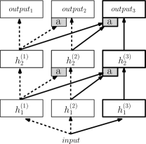
These modelling decisions are informed by our desire to: (1) solve $K$ independent tasks at the end of training; (2) accelerate learning via transfer when possible; and (3) avoid catastrophic forgetting.

In the standard pretrain-and-finetune paradigm, there is often an implicit assumption of “overlap” between the tasks. Finetuning is efficient in this setting, as parameters need only be adjusted slightly to the target domain, and often only the top layer is retrained [23]. In contrast, we make no assumptions about the relationship between tasks, which may in practice be orthogonal or even adversarial. While the finetuning stage could potentially unlearn these features, this may prove difficult. Progressive networks side-step this issue by allocating a new column for each new task, whose weights are initialized randomly. Compared to the task-relevant initialization of pretraining, columns in progressive networks are free to reuse, modify or ignore previously learned features via the lateral connections. As the lateral connections $U_{i}^{(k:j)}$ are only from column $k$ to columns $j<k$, previous columns are not affected by the newly learned features in the forward pass. Because also the parameters $\{\Theta^{(j)};j<k\}$ are kept frozen (i.e. are constants for the optimizer) when training $\Theta^{(k)}$, there is no interference between tasks and hence no catastrophic forgetting.

Application to Reinforcement Learning.

Although progressive networks are widely applicable, this paper focuses on their application to deep reinforcement learning. In this case, each column is trained to solve a particular Markov Decision Process (MDP): the $k$-th column thus defines a policy $\pi^{(k)}(a\mid s)$ taking as input a state $s$ given by the environment, and generating probabilities over actions $\pi^{(k)}(a\mid s):=h_{L}^{(k)}(s)$. At each time-step, an action is sampled from this distribution and taken in the environment, yielding the subsequent state. This policy implicitly defines a stationary distribution $\rho_{\pi^{(k)}}(s,a)$ over states and actions.

Adapters.

In practice, we augment the progressive network layer of Equation 2 with non-linear lateral connections which we call adapters. They serve both to improve initial conditioning and perform dimensionality reduction. Defining the vector of anterior features $h_{i-1}^{(<k)}=[h_{i-1}^{(1)}\cdots h_{i-1}^{(j)}\cdots h_{i-1}^{(k-1)}]$ of dimensionality $n_{i-1}^{(<k)}$, in the case of dense layers, we replace the linear lateral connection with a single hidden layer MLP. Before feeding the lateral activations into the MLP, we multiply them by a learned scalar, initialized by a random small value. Its role is to adjust for the different scales of the different inputs. The hidden layer of the non-linear adapter is a projection onto an $n_{i}$ dimensional subspace. As the index $k$ grows, this ensures that the number of parameters stemming from the lateral connections is in the same order as $\left|\Theta^{(1)}\right|$. Omitting bias terms, we get:

$$h_{i}^{(k)}=\sigma\left(W_{i}^{(k)}h_{i-1}^{(k)}+U_{i}^{(k:j)}\sigma(V_{i}^{(k:j)}\alpha_{i-1}^{(<k)}h_{i-1}^{(<k)})\right),$$ (2)

where $V_{i}^{(k:j)}\in\mathbb{R}^{n_{i-1}\times n_{i-1}^{(<k)}}$ is the projection matrix. For convolutional layers, dimensionality reduction is performed via $1\times 1$ convolutions [10].

Limitations.

Progressive networks are a stepping stone towards a full continual learning agent: they contain the necessary ingredients to learn multiple tasks, in sequence, while enabling transfer and being immune to catastrophic forgetting. A downside of the approach is the growth in number of parameters with the number of tasks. The analysis of Appendix 2 reveals that only a fraction of the new capacity is actually utilized, and that this trend increases with more columns. This suggests that growth can be addressed, e.g. by adding fewer layers or less capacity, by pruning [9], or by online compression [17] during learning. Furthermore, while progressive networks retain the ability to solve all $K$ tasks at test time, choosing which column to use for inference requires knowledge of the task label. These issues are left as future work.

3 Transfer Analysis

Unlike finetuning, progressive nets do not destroy the features learned on prior tasks. This enables us to study in detail which features and at which depth transfer actually occurs. We explored two related methods: an intuitive, but slow method based on a perturbation analysis, and a faster analytical method derived from the Fisher Information [2].

Average Perturbation Sensitivity (APS).

To evaluate the degree to which source columns contribute to the target task, we can inject Gaussian noise at isolated points in the architecture (e.g. a given layer of a single column) and measure the impact of this perturbation on performance. A significant drop in performance indicates that the final prediction is heavily reliant on the feature map or layer. We find that this method yields similar results to the faster Fisher-based method presented below. We thus relegate details and results of the perturbation analysis to the appendix.

Average Fisher Sensitivity (AFS).

We can get a local approximation to the perturbation sensitivity by using the Fisher Information matrix [2]. While the Fisher matrix is typically computed with respect to the model parameters, we compute a modified diagonal Fisher $\hat{F}$ of the network policy $\pi$ with respect to the normalized activations at each layer $\hat{h}_{i}^{(k)}$. For convolutional layers, we define $\hat{F}$ to implicitly perform a summation over pixel locations. $\hat{F}$ can be interpreted as the sensitivity of the policy to small changes in the representation. We define the diagonal matrix $\hat{F}$, having elements $\hat{F}(m,m)$, and the derived Average Fisher Sensitivity (AFS) of feature $m$ in layer $i$ of column $k$ as:

$$\hat{F}_{i}^{(k)} =\mathbb{E}_{\rho(s,a)}\left[\frac{\partial\log\pi}{\partial\hat{h}_{i}^{(k)}}\,\frac{\partial\log\pi}{\partial\hat{h}_{i}^{(k)}}^{T}\right] \text{AFS}(i,k,m) =\frac{\hat{F}_{i}^{(k)}(m,m)}{\sum_{k}\hat{F}_{i}^{(k)}(m,m)}$$

where the expectation is over the joint state-action distribution $\rho(s,a)$ induced by the progressive network trained on the target task. In practice, it is often useful to consider the AFS score per-layer $\text{AFS}(i,k)=\sum_{m}\text{AFS}(i,k,m)$, i.e. summing over all features of layer $i$. The AFS and APS thus estimate how much the network relies on each feature or column in a layer to compute its output.

4 Related Literature

There exist many different paradigms for transfer and multi-task reinforcement learning, as these have long been recognized as critical challenges in AI research [15, 19, 20]. Many methods for transfer learning rely on linear and other simple models (e.g. [18]), which is a limiting factor to their applicability. Recently, there have been new methods proposed for multi-task or transfer learning with deep RL: [22, 17, 14]. In this work we present an architecture for deep reinforcement learning that in sequential task regimes that enables learning without forgetting while supporting individual feature transfer from previous learned tasks.

Pretraining and finetuning was proposed in [7] and applied to transfer learning in [4, 11], generally in unsupervised-to-supervised or supervised-to-supervised settings. The actor-mimic approach [14] applied these principles to reinforcement learning, by fine-tuning a DQN multi-task network on new Atari games and showing that some responded with faster learning, while others did not. Progressive networks differ from the finetuning direction substantially, since capacity is added as new tasks are learned.

Progressive nets are related to the incremental and constructive architectures proposed in neural network literature. The cascade-correlation architecture was designed to eliminate forgetting while incrementally adding and refining feature extractors [6]. Auto-encoders such as [24] use incremental feature augmentation to track concept drift, and deep architectures such as [16] have been designed that specifically support feature transfer. More recently, in [1], columns are separately trained on individual noise types, then linearly combined, and [5] use columns for image classification. The block-modular architecture of [21] has many similarities to our approach but focuses on a visual discrimination task. The progressive net approach, in contrast, uses lateral connections to access previously learned features for deep compositionality. It can be used in any sequential learning setting but is especially valuable in RL.

5 Experiments

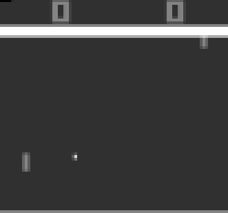
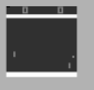
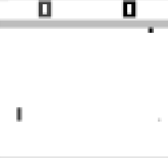
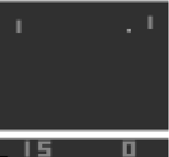
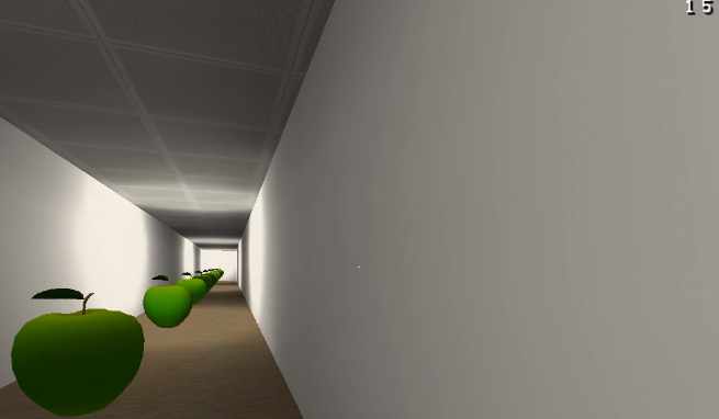
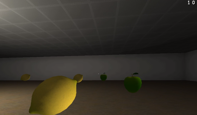
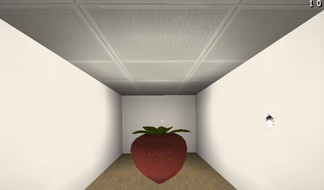
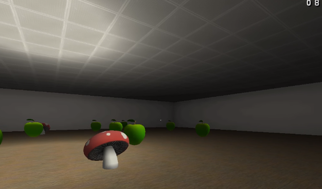
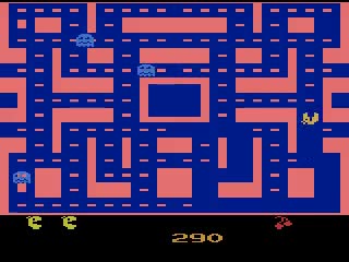
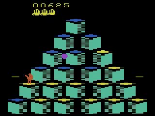
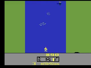
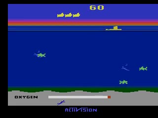
We evaluate progressive networks across three different RL domains. First, we consider synthetic versions of Pong, altered to have visual or control-level similarities. Next, we experiment broadly with random sequences of Atari games and perform a feature-level transfer analysis. Lastly, we demonstrate performance on a set of 3D maze games. Fig. 2 shows examples from selected tasks.

(a) Pong variants

(b) Labyrinth games

(c) Atari games

Figure 2: Samples from different task domains: (a) Pong variants include flipped, noisy, scaled, and recoloured transforms; (b) Labyrinth is a set of 3D maze games with diverse level maps and diverse positive and negative reward items; (c) Atari games offer a more challenging setting for transfer.

5.1 Setup

We rely on the Async Advantage Actor-Critic (A3C) framework introduced in [13]. Compared to DQN [12], the model simultaneously learns a policy and a value function for predicting expected future rewards. A3C is trained on CPU using multiple threads and has been shown to converge faster than DQN on GPU. This made it a more natural fit for the large amount of sequential experiments required for this work.

We report results by averaging the top 3 out of 25 jobs, each having different seeds and random hyper-parameter sampling. Performance is evaluated by measuring the area under the learning curve (average score per episode during training), rather than final score. The transfer score is then defined as the relative performance of an architecture compared with a single column baseline, trained only on the target task (baseline 1). We present transfer score curves for selected source-target games, and summarize all such pairs in transfer matrices. Models and baselines we consider are illustrated in Figure 3. Details of the experimental setup are provided in section 3 of the Appendix.

Figure 3: Illustration of different baselines and architectures. Baseline 1 is a single column trained on the target task; baseline 2 is a single column, pretrained on a source task and finetuned on the target task (output layer only); baseline 3 is the same as baseline 2 but the whole model is finetuned; and baseline 4 is a 2 column progressive architecture, with previous column(s) initialized randomly and frozen.

5.2 Pong Soup

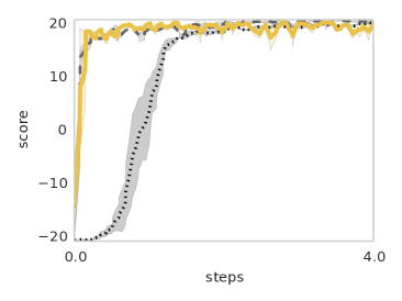
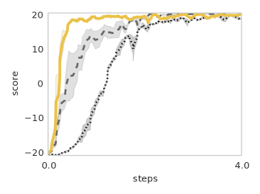
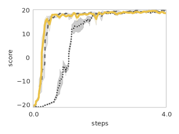
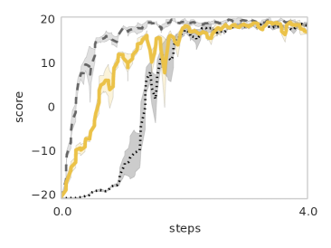
The first evaluation domain is a set of synthetic variants of the Atari game of Pong ("Pong Soup") where the visuals and gameplay have been altered, thus providing a setting where we can be confident that there are transferable aspects of the tasks. The variants are Noisy (frozen Gaussian noise is added to the inputs); Black (black background); White (white background); Zoom (input is scaled by 75% and translated); V-flip, H-flip, and VH-flip (input is horizontally and/or vertically flipped). Example frames are shown in Fig. 2. The results of training two columns on the Pong variants, including all relevant baselines are shown in Figure 4. Transfer scores are summarized over all target tasks in Table 1.

Figure 4: (a) Transfer matrix. Colours indicate transfer scores (clipped at 2). For progressive nets, the first column is trained on Pong, Noisy, or H-flip (table rows); the second column is trained on each of the other pong variants (table columns). (b) Example learning curves.

We can make several observations from these results. Baseline 2 (single column, only output layer is finetuned; see Fig. 3) fails to learn the target task in most experiments and thus has negative transfer. This approach is quite standard in supervised learning settings, where features from ImageNet-trained nets are routinely repurposed for new domains. As expected, we observe high positive transfer with baseline 3 (single column, full finetuning), a well established paradigm for transfer. Progressive networks outperform this baseline however in terms of both median and mean score, with the difference being more pronounced for the latter. As the mean is more sensitive to outliers, this suggests that progressive networks are better able to exploit transfer when transfer is possible (i.e. when source and target domains are compatible). Fig. 4 (b) lends weight to this hypothesis, where progressive networks are shown to significantly outperform the baselines for particular game pairs. Progressive nets also compare favourably to baseline 4, confirming that progressive nets are indeed taking advantage of the features learned in previous columns.

Detailed analysis

Figure 5: (a) Transfer analysis for 2-column nets on Pong variants. The relative sensitivity of the network’s outputs on the columns within each layer (the AFS) is indicated by the darkness of shading. (b) AFS values for the 8 feature maps of conv. 1 of a 1-column Pong net. Only one feature map is effectively used by the net; the same map is also used by the 2-column versions. Below: spatial filter components (red = positive, blue = negative). (c) Activation maps of the filter in (b) from example states of the four games.

We use the metric derived in Sec. 3 to analyse what features are being transferred between Pong variants. We see that when switching from Pong to H-Flip, the network reuses the same components of low and mid-level vision (the outputs of the two convolutional layers; Figure 5a). However, the fully connected layer must be largely re-learned, as the policy relevant features of the task (the relative locations/velocities of the paddle and ball) are now in a new location. When switching from Pong to Zoom, on the other hand, low-level vision is reused for the new task, but new mid-level vision features are learned. Interestingly, only one low-level feature appears to be reused: (see Fig. 5b): this is a spatio-temporal filter with a considerable temporal DC component. This appears sufficient for detecting both ball motion and paddle position in the original, flipped, and zoomed Pongs.

Finally, when switching from Pong to Noisy, some new low-level vision is relearned. This is likely because the first layer filter learned on the clean task is not sufficiently tolerant to the added noise. In contrast, this problem does not apply when moving from Noisy to Pong (Figure 5a, rightmost column), where all of vision transfers to the new task.

5.3 Atari Games

We next investigate feature transfer between randomly selected Atari games [3]. This is an interesting question, because the visuals of Atari games are quite different from each other, as are the controls and required strategy. Though games like Pong and Breakout are conceptually similar (both involve hitting a ball with a paddle), Pong is vertically aligned while Breakout is horizontal: a potentially insurmountable feature-level difference. Other Atari game pairs have no discernible overlap, even at a conceptual level.

Figure 6: Transfer scores and example learning curves for Atari target games, as per Figure 4.

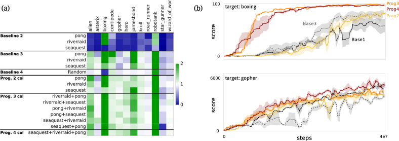
To this end we start by training single columns on three source games (Pong, River Raid, and Seaquest) and assess if the learned features transfer to a different subset of randomly selected target games (Alien, Asterix, Boxing, Centipede, Gopher, Hero, James Bond, Krull, Robotank, Road Runner, Star Gunner, and Wizard of Wor). We evaluate progressive networks with 2, 3 and 4 columns, comparing to the baselines of Figure 3). The transfer matrix and selected transfer curves are shown in Figure 6, and the results summarized in Table 1.

Across all games, we observe from Fig. 6, that progressive nets result in positive transfer in 8 out of 12 target tasks, with only two cases of negative transfer. This compares favourably to baseline 3, which yields positive transfer in only 5 of 12 games. This trend is reflected in Table 1, where progressive networks convincingly outperform baseline 3 when using additional columns. This is especially promising as we show in the Appendix that progressive network use a diminishing amount of capacity with each added column, pointing a clear path to online compression or pruning as a means to mitigate the growth in model size.

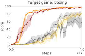
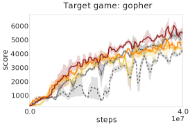
Now consider the specific sequence Seaquest-to-Gopher, an example of two dissimilar games. Here, the pretrain/finetune paradigm (baseline 3) exhibits negative transfer, unlike progressive networks (see Fig.6b, bottom), perhaps because they are more able to ignore the irrelevant features. For the sequence Seaquest[+River Raid][+Pong]-to-Boxing, using additional columns in the progressive networks can yield a significant increase in transfer (see Fig. 6b, top).

	Pong Soup		Atari		Labyrinth
	Mean (%)	Median (%)	Mean (%)	Median (%)	Mean (%)	Median (%)
Baseline 1	100	100	100	100	100	100
Baseline 2	35	7	41	21	88	85
Baseline 3	181	160	133	110	235	112
Baseline 4	134	131	96	95	185	108
Progressive 2 col	209	169	132	112	491	115
Progressive 3 col	222	183	140	111	—	—
Progressive 4 col	—	—	141	116	—	—

Table 1: Transfer percentages in three domains. Baselines are defined in Fig. 3.

Detailed Analysis

Figure 6 demonstrates that both positive and negative transfer is possible with progressive nets. To differentiate these cases, we consider the Average Fisher Sensitivity for the 3 column case (e.g., see Fig. 7a). A clear pattern emerges amongst these and other examples: the most negative transfer coincides with complete dependence on the convolutional layers of the previous columns, and no learning of new visual features in the new column. In contrast, the most positive transfer occurs when the features of the first two columns are augmented by new features. The statistics across all 3-column nets (Figure 7b) show that positive transfer in Atari occurs at a "sweet spot" between heavy reliance on features from the source task, and heavy reliance on all new features for the target task.

Figure 7: (a) AFS scores for 3-column nets with lowest (left) and highest (right) transfer scores on the 12 target Atari games. (b) Transfer statistics across 72 three-column nets, as a function of the mean AFS across the three convolutional layers of the new column (i.e. how much new vision is learned).

At first glance, this result appears unintuitive: if a progressive net finds a valuable feature set from a source task, shouldn’t we expect a high degree of transfer? We offer two hypotheses. First, this may simply reflect an optimization difficulty, where the source features offer fast convergence to a poor local minimum. This is a known challenge in transfer learning [20]: learned source tasks confer an inductive bias that can either help or hinder in different cases. Second, this may reflect a problem of exploration, where the transfered representation is "good enough" for a functional, but sub-optimal policy.

5.4 Labyrinth

The final experimental setting for progressive networks is Labyrinth, a 3D maze environment where the inputs are rendered images granting partial observability and the agent outputs discrete actions, including looking up, down, left, or right and moving forward, backwards, left, or right. The tasks as well as the level maps are diverse and involve getting positive scores for ‘eating’ good items (apples, strawberries) and negative scores for eating bad items (mushrooms, lemons). Details can be found in the appendix. While there is conceptual and visual overlap between the different tasks, the tasks present a challenging set of diverse game elements (Figure 2).

Figure 8: Transfer scores and example learning curves for Labyrinth tasks. Colours indicate transfer (clipped at 2). The learning curves show two examples of two-column progressive performance vs. baselines 1 and 3.

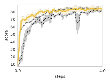
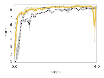
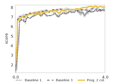
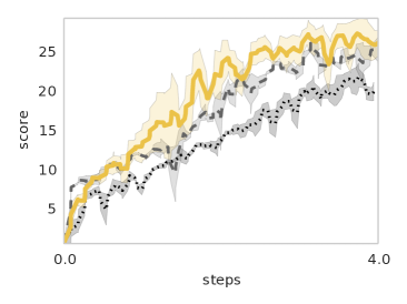
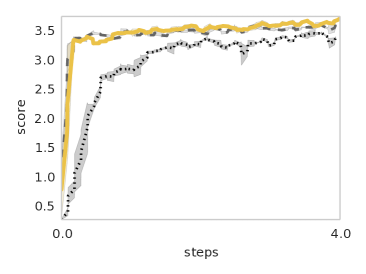
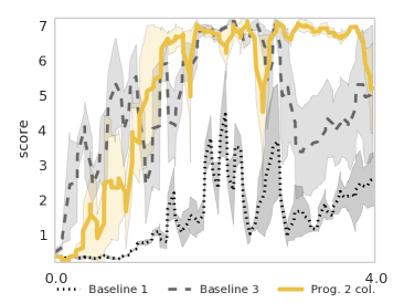
As in the other domains, the progressive approach yields more positive transfer than any of the baselines (see Fig. 8a and Table 1). We observe less transfer on the Seek Track levels, which have dense reward items throughout the maze and are easily learned. Note that even for these easy cases, baseline 2 shows negative transfer because it cannot learn new low-level visual features, which are important because the reward items change from task to task. The learning curves in Fig. 8b exemplify the typical results seen in this domain: on simpler games, such as Track 1 and 2, learning is rapid and stable by all agents. On more difficult games, with more complex game structure, the baselines struggle and progressive nets have an advantage.

6 Conclusion

Continual learning, the ability to accumulate and transfer knowledge to new domains, is a core characteristic of intelligent beings. Progressive neural networks are a stepping stone towards continual learning, and this work has demonstrated their potential through experiments and analysis across three RL domains, including Atari, which contains orthogonal or even adversarial tasks. We believe that we are the first to show positive transfer in deep RL agents within a continual learning framework. Moreover, we have shown that the progressive approach is able to effectively exploit transfer for compatible source and task domains; that the approach is robust to harmful features learned in incompatible tasks; and that positive transfer increases with the number of columns, thus corroborating the constructive, rather than destructive, nature of the progressive architecture.

Supplementary Material

Appendix A Perturbation Analysis

We explored two related methods for analysing transfer in progressive networks. One based on Fisher information yields the Average Fisher Sensitivity (AFS) and is described in Section 3 of the paper. We describe the second method based on perturbation analysis in this appendix, as it proved too slow to use at scale. Given its intuitive appeal however, we provide details of the method along with results on Pong Variants (see Section 5.2), as a means to corroborate the AFS score.

Our perturbation analysis aims to estimate which components of the source columns materially contribute to the performance of the final column on the target tasks. To this end, we injected Gaussian noise into each of the (post-ReLU) hidden representations, with a new sample on every forward pass, and calculated the average effect of these perturbations on the game score over 10 episodes. We did this at a coarse scale, by adding noise across all features of a given layer, though a fine scale analysis is also possible per feature (map). In order to be invariant to any arbitrary scale factors in the network weights, we scale the noise variance proportional to the variance of the activations in each feature map and fully-connected neuron. Scaling the variance in this manner is analogous to computing the Fisher w.r.t. normalized activations for the AFS score.

Figure 9: (a) Perturbation analysis for the two second-layer convolutional representations in the two columns of the Pong/Pong-noise net. Blue: adding noise to second convolutional layer from column 1; green: from column 2. Grey line determines critical noise magnitude for each representation, $\sigma_{i}^{2}$. (b-c) Comparison of per-layer sensitivities obtained using the APS method (b) and the AFS method (c; as per main text). These are highly similar.

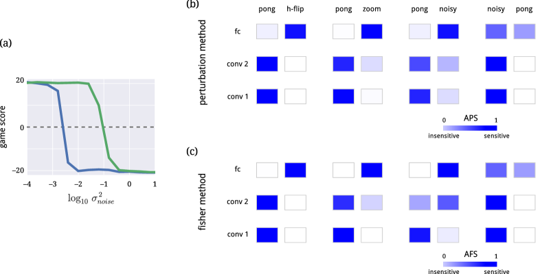
Define ${\Lambda_{i}^{(k)}}=1/\sigma_{i}^{2(k)}$ as the precision of the noise injected at layer $i$ of column $k$, which results in a $50\%$ drop in performance. The Average Perturbation Sensitivity (APS) for this layer is simply:

$$\text{APS}(i,k)=\frac{\Lambda_{i}^{(k)}}{\sum_{k}\Lambda_{i}^{(k)}}$$ (3)

Note that this value is normalized across columns for a given layer. The APS score can thus be interpreted as the responsibility of each column in a given layer to final performance. The APS score of 2-column progressive networks trained on Pong Variants is shown in Fig9 (b). These clearly corroborate the AFS shown in (c).

Appendix B Compressibility of Progressive Networks

As described in the main text, one of the limitations of progressive networks is the growth in the size of the network with added tasks. In the basic approach we pursue in the main text, the number of hidden units and feature maps grows linearly with the number of columns, and the number of parameters grows quadratically.

Here, we sought to determine the degree to which this full capacity is actually used by the network. We leveraged the Average Fisher Sensitivity measure to study how increasing the number of columns in the Atari task set changes the need for additional resources. In Figure 10a, we measure the average fractional use of existing feature maps in a given layer (here, layer 2). We do this for each network by concatenating the per-feature-map AFS values from all source columns in this layer, sorting the values to produce a spectrum, and then averaging across networks. We find that as the number of columns increases, the average spectrum becomes sparser: the network relies on a smaller proportion of features from the source columns. Similar results were found for all layers.

Similarly, in Figure 10b, we measure the capacity required in the final added column as a function of the total number of columns. Again, we measure the spectrum of AFS values in an example layer, but here from only the final column. As the progressive network grows, the new column’s features are both less important overall (indicated by the declining area under the graph), and have a sparser AFS spectrum. Combined, these results suggest that significant pruning of lateral connections is possible, and the quadratic growth of parameters might be contained.

Figure 10: (a) Spectra of AFS values (for layer 2) across all feature maps from source columns, for the Atari dataset. The spectra show the range of AFS values, and are averaged across networks. While the 2 column / 3 column / 4 column nets all have different values of $N_{maps}$ (here, 12, 24, and 36 respectively), these have been dilated to fit the same axis to show the proportional use of these maps. (b) Spectra of AFS values (for layer 2) for the feature maps from only the final column.

Appendix C Setup Details

In our grid we sample hyper-parameters from categorical distributions:

• Learning rate was sampled from $\{10^{-3},5\cdot 10^{-4},10^{-4}\}$.

• Strength of the entropy regularization from $\{10^{-2},10^{-3},10^{-4}\}$

• Gradient clipping cut-off from $\{20,40\}$

• scalar multiplier on the lateral feature is initialized randomly to one from $\{1,10^{-1},10^{-2}\}$

For the Atari experiments we used a model with 3 convolutional layers followed by a fully connected layer and from which we predict the policy and value function. The convolutional layers are as follows. All have 12 feature maps. The first convolutional layer has a kernel of size 8x8 and a stride of 4x4. The second layer has a kernel of size 4 and a stride of 2. The last convolutional layer has size 3x4 with a stride of 1. The fully connected layer has 256 hidden units.

Learning follows closely the paradigm described in [13]. We use 16 workers and the same RMSProp algorithm without momentum or centring of the variance. The score for each point of a training curve is the average over all the episodes the model gets to finish in $25e4$ environment steps.

The whole experiments are run for a maximum of $1.6e8$ environment step. The agent has an action repeat of 4 as in [13], which means that for 4 consecutive steps the agent will use the same action picked at the beginning of the series. For this reason through out the paper we actually report results in terms of agent perceived steps rather than environment steps. That is, the maximal number of agent perceived step that we do for any particular run is $4e7$.

Appendix D Learning curves

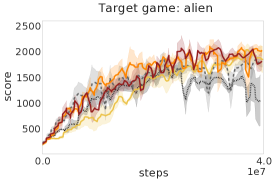
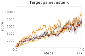
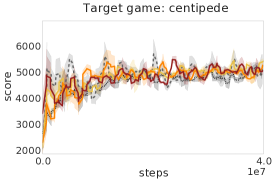
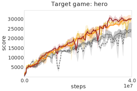
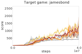
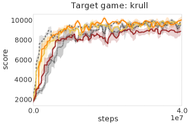
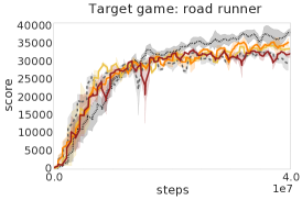
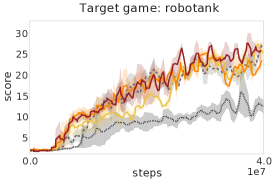
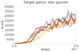
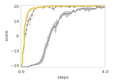
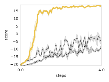
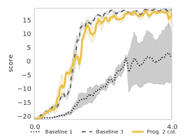
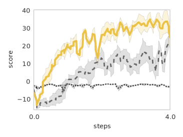
Figure 11 shows training curves for all the target games in the Atari domain. We plot learning curves for two column, three column and four column progressive networks alongside Baseline 3 (gray dashed line), a model pretrained on Seaquest and then finetuned on the particular target game and Baseline 1 (gray dotted line), where a single column is trained on the source game Seaquest.

Figure 11: Training curves for transferring to the target games after seeing first Seaquest followed by River Raid and lastly Pong. For the baselines, the source game used for pretraining is Seaquest.

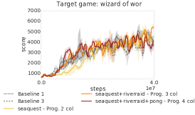We can see that overall baseline 3 performs well. However there are situations when having features learned from more previous task actually helps with transfer (e.g. when target game is Boxing).

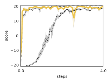
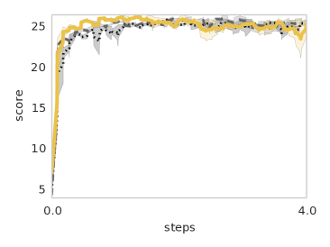
Figure 12 shows how two-column progressive networks perform as compared to Baseline 3 (gray dashed line), a model pretrained on the source game, here standard Pong, and then finetuned on a particular target game, and Baseline 1 (black dotted line), where a single column is trained on standard Pong. Figure 13 shows two-column progressive networks and baselines on Labyrinth tasks; the source game was Maze Y.

Target: Pong	Target: Black
Target: H-flip	Target: HV-flip
Target: Noisy	Target: V-flip
Target: White	Target: Zoom

Figure 12: Training curves for transferring to 8 target games after learning standard Pong first.

Target: Track 1	Target: Track 2
Target: Track 3	Target: Track 4
Target: Avoid 1	Target: Avoid 2
Target: Maze Y	Target: Maze M

Figure 13: Training curves for transferring to 8 target games after learning Maze Y first.

Appendix E Labyrinth

Section 5.4 evaluates progressive networks on foraging tasks in complex 3D maze environments. Positive rewards are given to the agent for collecting apples and strawberries, and negative rewards for mushrooms and lemons. Episodes terminate when either all (positive) rewards are collected, or after a fixed time interval.

Levels differ in their maze layout, the type of items present and the sparsity of the reward structure. The levels we employed can be characterized as follows:

• Seek Track 1: simple corridor with many apples

• Seek Track 2: U-shaped corridor with many strawberries

• Seek Track 3: $\Omega$-shaped, with $90^{o}$ turns, with few apples

• Seek Track 4: $\Omega$-shaped, with $45^{o}$ turns, with few apples

• Seek Avoid 1: large square room with apples and lemons

• Seek Avoid 2: large square room with apples and mushrooms

• Seek Maze M : M-shaped maze, with apples at dead-ends

• Seek Maze Y : Y-shaped maze, with apples at dead-ends

References

- [1] Forest Agostinelli, Michael R Anderson, and Honglak Lee. Adaptive multi-column deep neural networks with application to robust image denoising. In Advances in Neural Information Processing Systems, 2013.
- [2] Shun-ichi Amari. Natural gradient works efficiently in learning. Neural Computation, 1998.
- [3] M. G. Bellemare, Y. Naddaf, J. Veness, and M. Bowling. The arcade learning environment: An evaluation platform for general agents. Journal of Artificial Intelligence Research (JAIR), 47:253–279, 2013.
- [4] Yoshua Bengio. Deep learning of representations for unsupervised and transfer learning. In JMLR: Workshop on Unsupervised and Transfer Learning, 2012.
- [5] Dan C. Ciresan, Ueli Meier, and Jürgen Schmidhuber. Multi-column deep neural networks for image classification. In Conf. on Computer Vision and Pattern Recognition, 2012.
- [6] Scott E. Fahlman and Christian Lebiere. The cascade-correlation learning architecture. In Advances in Neural Information Processing Systems, 1990.
- [7] G. E. Hinton and R. R. Salakhutdinov. Reducing the dimensionality of data with neural networks. Science, 313(5786):504–507, July 2006.
- [8] Goeff Hinton, Oriol Vinyals, and Jeff Dean. Distilling the knowledge in a neural network. CoRR, abs/1503.02531, 2015.
- [9] Yann LeCun, John S. Denker, and Sara A. Solla. Optimal brain damage. In Advances in Neural Information Processing Systems, 1990.
- [10] Min Lin, Qiang Chen, and Shuicheng Yan. Network in network. In Proc. of Int’l Conference on Learning Representations (ICLR), 2013.
- [11] G. Mesnil, Y. Dauphin, X. Glorot, S. Rifai, Y. Bengio, I. Goodfellow, E. Lavoie, X. Muller, G. Desjardins, D. Warde-Farley, P. Vincent, A. Courville, and J. Bergstra. Unsupervised and transfer learning challenge: a deep learning approach. In JMLR W& CP: Proc. of the Unsupervised and Transfer Learning challenge and workshop, volume 27, 2012.
- [12] V. Mnih, Kk Kavukcuoglu, D. Silver, A. Rusu, J. Veness, M. Bellemare, A. Graves, M. Riedmiller, A. Fidjeland, G. Ostrovski, S. Petersen, C. Beattie, A. Sadik, I. Antonoglou, H. King, D. Kumaran, D. Wierstra, S. Legg, and D. Hassabis. Human-level control through deep reinforcement learning. Nature, 518(7540):529–533, 2015.
- [13] Volodymyr Mnih, Adrià Puigdomènech Badia, Mehdi Mirza, Alex Graves, Timothy P. Lillicrap, Tim Harley, David Silver, and Koray Kavukcuoglu. Asynchronous methods for deep reinforcement learning. In Int’l Conf. on Machine Learning (ICML), 2016.
- [14] Emilio Parisotto, Lei Jimmy Ba, and Ruslan Salakhutdinov. Actor-mimic: Deep multitask and transfer reinforcement learning. In Proc. of Int’l Conference on Learning Representations (ICLR), 2016.
- [15] Mark B. Ring. Continual Learning in Reinforcement Environments. R. Oldenbourg Verlag, 1995.
- [16] Artem Rozantsev, Mathieu Salzmann, and Pascal Fua. Beyond sharing weights for deep domain adaptation. CoRR, abs/1603.06432, 2016.
- [17] A. Rusu, S. Colmenarejo, Ç. Gülçehre, G. Desjardins, J. Kirkpatrick, R. Pascanu, V. Mnih, K. Kavukcuoglu, and R. Hadsell. Policy distillation. abs/1511.06295, 2016.
- [18] Paul Ruvolo and Eric Eaton. Ella: An efficient lifelong learning algorithm. In Proceedings of the 30th International Conference on Machine Learning (ICML-13), June 2013.
- [19] Daniel L. Silver, Qiang Yang, and Lianghao Li. Lifelong machine learning systems: Beyond learning algorithms. In AAAI Spring Symposium: Lifelong Machine Learning, 2013.
- [20] Matthew E. Taylor and Peter Stone. An introduction to inter-task transfer for reinforcement learning. AI Magazine, 32(1):15–34, 2011.
- [21] Alexander V. Terekhov, Guglielmo Montone, and J. Kevin O’Regan. Knowledge Transfer in Deep Block-Modular Neural Networks, pages 268–279. Springer International Publishing, Cham, 2015.
- [22] C. Tessler, S. Givony, T. Zahavy, D. J. Mankowitz, and S. Mannor. A Deep Hierarchical Approach to Lifelong Learning in Minecraft. ArXiv e-prints, 2016.
- [23] Jason Yosinski, Jeff Clune, Yoshua Bengio, and Hod Lipson. How transferable are features in deep neural networks? In Advances in Neural Information Processing Systems, pages 3320–3328, 2014.
- [24] Guanyu Zhou, Kihyuk Sohn, and Honglak Lee. Online incremental feature learning with denoising autoencoders. In Proc. of Int’l Conf. on Artificial Intelligence and Statistics (AISTATS), pages 1453–1461, 2012.