Abstract

Redundancy is related to the amount of functionality that the structure can sustain in the worst-case scenario of structural degradation. This paper proposes a widely-applicable concept of redundancy optimization of finite-dimensional structures. The concept is consistent with the robust structural optimization, as well as the quantitative measure of structural redundancy based on the information-gap theory. A derivative-free algorithm is proposed based on the sequential quadratic programming (SQP) method, where we use the finite-difference method with adaptively varying the difference increment. Preliminary numerical experiments show that an optimal solution of the redundancy optimization problem possibly has multiple worst-case scenarios.

Keywords

Robustness; redundancy; resilience; uncertainty; derivative-free optimization; simplex gradient.

1 Introduction

Since real-world structures inevitably encounter various uncertainties, robustness and redundancy are crucial concepts in structural design. Robust optimization of structures has been studied extensively; see, e.g., [3, 6, 9, 10, 12, 24, 26, 29], and the references therein. In contrast, study on design methodology of structures considering redundancy property is very limited. Mohr et al. [18] applied the notion of redundancy in the coding theory to truss optimization. Mousavi and Gardoni [19] considered the conditional probability of failure of each structural component given failure of the structure, and proposed to minimize the difference between the maximum and minimum values of these conditional probabilities. Also, optimization problems of fail-safe structures are relevant to the problem studied in this paper. Sun et al. [25] and Nguyen and Arora [20] defined a damage condition as complete or partial damage to selected structural components. They specified several damage scenarios a priori, and imposed the performance constraints on all the damaged scenarios, as well as on the intact scenario. For continuum-based topology optimization, Jansen et al. [13] considered the effect of local failure. As a simple model of local failure, they supposed that the material stiffness in a patch with a specified shape vanishes. The location of patch is assumed to be unknown in advance, and the compliance in the worst-case scenario is minimized to obtain a fail-safe structure.

This paper attempts to present a widely-applicable concept of redundancy optimization of finite-dimensional structures. Several definitions of redundancy of structures have been proposed; see, e.g., [4, 5, 8, 15, 17, 22, 30, 31], and the references therein. Among others, in this paper we adopt the strong redundancy [15], which is a quantitative measure of structural redundancy based on the information-gap theory [1]. The strong redundancy of a given structural design is defined as the greatest deficiency that can arise at any place in the structure, without violating the performance constraint. Thus the concept of strong redundancy can fully address uncertainty in future structural degradation. Moreover, it has flexibility to incorporate diverse structural performances, unlike most of other redundancy measures that consider only the ultimate strength or the collapse load as the structural performance of interest.

In the redundancy optimization problem proposed in this paper, we specify only the upper bound for the number of damaged structural components, denoted $\alpha$, while the damaged structural components themselves are considered unknown (or, uncertain). Then we formulate a worst-case design optimization problem. Namely, we optimize the objective function evaluated in the worst-case scenario of structural degradation. This methodology shares a common framework with extensively studied robust compliance optimization of structures with a non-probabilistic modeling of uncertainty. There, the worst-case compliance (i.e., the maximum value of the compliance) is minimized, when the static external load or the structural geometry is assumed to be uncertain [3, 6, 9, 10, 12, 24, 26, 29].

As a concrete example of the redundancy optimization, attention of this paper is focused on maximization of the worst-case limit load factor of a truss structure. When $\alpha=0$, i.e., no redundancy is required, the redundancy optimization reverts to the classical limit design (optimal plastic design). For $\alpha\geq 1$, an optimal solution of the redundancy optimization is statically indeterminate, unlike the limit design. For given $\alpha$ and structural design, the worst-case limit load factor can be computed via mixed-integer linear programming (MILP) [14]; see also Tangaramvong et al. [27]. As a substitute of the gradient of the worst-case limit load factor, we employ the simplex gradient (also called the stencil gradient) that is often used in derivative-free optimization methods [7, 16]. More concretely, we compute the finite-difference gradient with decreasing a difference increment as the optimization procedure progresses. Making use of this approximated gradient, we propose a derivative-free method based on the sequential quadratic programming (SQP) for solving the redundancy optimization problem.

The paper is organized as follows. First, a concept of redundancy optimization of structures is defined. We also discuss the relation between the redundancy optimization and the robust optimization. The following section presents a derivative-free optimization method that combines SQP and the finite-difference gradient with a varying difference increment. Then, we apply the algorithm to simple problem instances to investigate some properties of the obtained solutions. Some conclusions are drawn at the end of the paper.

A few words regarding notation. We use ^⊤ to denote the transpose of a vector or a matrix. For two vectors $\boldsymbol{x}=(x_{i})\in\mathbb{R}^{n}$ and $\boldsymbol{s}=(s_{i})\in\mathbb{R}^{n}$, we write $\boldsymbol{x}\geq\boldsymbol{s}$ if $x_{i}\geq s_{i}$ $(i=1,\dots,n)$. Particularly, $\boldsymbol{x}\geq\boldsymbol{0}$ means $x_{i}\geq 0$ $(i=1,\dots,n)$. We use $\boldsymbol{1}=(1,1,\dots,1)^{\top}$ to denote the all-ones vector. The $\ell_{1}$-norm and the Euclidean norm of a vector $\boldsymbol{x}\in\mathbb{R}^{n}$ is denoted by $\|\boldsymbol{x}\|_{1}=\sum_{i=1}^{n}|x_{i}|$ and $\|\boldsymbol{x}\|=(\boldsymbol{x}^{\top}\boldsymbol{x})^{1/2}$, respectively. We use $\mathop{\mathrm{diag}}\nolimits(\boldsymbol{x})$ to denote the $n\times n$ diagonal matrix with a vector $\boldsymbol{x}\in\mathbb{R}^{n}$ on its diagonal. For a matrix $A\in\mathbb{R}^{m\times n}$, we use $A^{+}\in\mathbb{R}^{n\times m}$ and $\mathop{\mathrm{Ker}}\nolimits A$ to denote its Moore–Penrose pseudoinverse and nullspace, respectively. For $a$, $b\in\mathbb{R}$ satisfying $a<b$, we denote by $[a,b]$ and $]a,b[$ the closed and open intervals between $a$ and $b$, respectively.

2 Problem formulation

In this section we present a concept of redundancy optimization of structures, which is consistent with the widely accepted notion of robust structural optimization [3, 6, 10, 26, 29]. Also, it is naturally endowed with a qualitative measure of structural redundancy, called the strong redundancy [15].

Let $\boldsymbol{x}\in\mathbb{R}^{m}$ denote the vector of design variables, where $m$ is the number of the design variables. Consider structural performance $h(\boldsymbol{x})$ depending on structural design $\boldsymbol{x}$. A small value of $h(\boldsymbol{x})$ is preferred over a large value. The conventional optimization problem that maximizes the structural performance is formulated as follows:

$$\mathop{\mathrm{Min.}} h(\boldsymbol{x})$$ (1a)

$$\mathop{\mathrm{s.{\,}t.}} \boldsymbol{x}\in X.$$ (1b)

Here, $X\subseteq\mathbb{R}^{m}$ is the set of feasible design variables.

Example 1.

Consider a truss structure consisting of $m$ members. Let $\boldsymbol{x}$ be a nonnegative real vector, the $i$th component of which is the cross-sectional area of member $i$. We use $\lambda(\boldsymbol{x})$ to denote the limit load factor of the truss, and let $h(\boldsymbol{x})=-\lambda(\boldsymbol{x})$. A small value of $h(\boldsymbol{x})$ is worthy. A typical example of constraint $\boldsymbol{x}\in X$ has the form

$$X=\{\boldsymbol{x}\mid\boldsymbol{c}^{\top}\boldsymbol{x}\leq V,\ \boldsymbol{x}\geq\boldsymbol{0}\},$$ (2)

where $c_{i}$ is the undeformed length of member $i$ and $V$ is the specified upper bound for the structural volume. In this situation, problem (1) is the conventional limit design problem. $\blacksquare$

Example 2.

As in Example 1, consider a truss structure. Let $\boldsymbol{u}(\boldsymbol{x})$ denote the nodal displacement vector caused by the specified static external load. Consider the displacement constraints

$$|u_{j}(\boldsymbol{x})|\leq\bar{g}_{j},\quad j=1,\dots,k,$$ (3)

where $\bar{g}_{j}$ is a specified positive value and $k$ is the number of nodes for which the displacement constraint is considered. Let $h$ be

$$h(\boldsymbol{x})=\max\{|u_{1}(\boldsymbol{x})|-\bar{g}_{1},\dots,|u_{k}(\boldsymbol{x})|-\bar{g}_{k},0\}.$$

Namely, $h(\boldsymbol{x})$ measures violation of constraint (3), and $h(\boldsymbol{x})=0$ means that constraint (3) is satisfied. $\blacksquare$

Future structural damage is unknown in advance. Hence, based upon the information-gap theory [1], the strong redundancy [15] of design $\boldsymbol{x}$ is defined as the greatest deficiency that can arise at any place in the structure, without violating the performance constraint. In other words, the strong redundancy guarantees structural functionality in the worst-case scenario, when future structural damage is uncertain. Therefore, to increase redundancy it is natural to attempt to maximize the structural performance in the worst-case scenario of structural deficiency. Obviously, the worst-case scenario depends on the structural design.

For structural component $i$, we use binary variable $t_{i}$ that serves as a indicator of soundness. Specifically, the value of $t_{i}$ is defined by

$$t_{i}=\begin{dcases*}1&if member $i$ is intact,\\ 0&if member $i$ is damaged.\\ \end{dcases*}$$

Then vector $\boldsymbol{t}=(t_{1},\dots,t_{m})^{\top}$ expresses the scenario of deficiency that the structure suffers. In particular, the nominal scenario, which refers to the completely intact structure, corresponds to $\boldsymbol{t}=\boldsymbol{1}$. Following Kanno [14] and Kanno and Ben-Haim [15], we define the deficiency set by

$$T(\alpha)=\{\boldsymbol{t}\in\{0,1\}^{m}\mid\|\boldsymbol{t}-\boldsymbol{1}\|_{1}\leq\alpha\},$$

where $\alpha\geq 0$ is a parameter representing the level of structural damage. Namely, $T(\alpha)$ is the set of all scenarios in which the structure suffers degradation of at most an amount $\alpha$. From the definition, it is straightforward to see that $T(0)$ is a singleton consisting of the nominal scenario (i.e., $\boldsymbol{t}=\boldsymbol{1}$), and that $0\leq\alpha\leq\alpha^{\prime}$ implies $T(\alpha)\subseteq T(\alpha^{\prime})$.

Recall that the structural design is characterized by $\boldsymbol{x}$. We assume that a damaged structural component completely loses its functionality. Then the realization of the $i$th structural component is written as $t_{i}x_{i}$. Therefore, the set of all possible realizations of the structural design is given by

$$D(\boldsymbol{x};\alpha)=\{\mathop{\mathrm{diag}}\nolimits(\boldsymbol{t})\boldsymbol{x}\mid\boldsymbol{t}\in T(\alpha)\}.$$ (4)

Remark 1.

In (4) we assume a model that a damaged structural component is completely missing from the structure. Alternatively, we may suppose that structural components are diminishing only in part. Let $\gamma\in[0,1[$ be a constant representing the degree of damage. We assume that all members share same value of $\gamma$. Then the deficiency set is given by

$$D(\boldsymbol{x};\alpha)=\{\mathop{\mathrm{diag}}\nolimits(\boldsymbol{t}+\gamma(\boldsymbol{1}-\boldsymbol{t}))\boldsymbol{x}\mid\boldsymbol{t}\in T(\alpha)\}.$$

This model with $\alpha=1$ was considered in, e.g., [25]. Obviously, when $\gamma=0$, this model reverts to (4). $\blacksquare$

For given $\alpha\geq 0$ and $\boldsymbol{x}\in X$, define $h^{\mathrm{worst}}(\boldsymbol{x};\alpha)$ by

$$h^{\mathrm{worst}}(\boldsymbol{x};\alpha)=\max\{h(\boldsymbol{s})\mid\boldsymbol{s}\in D(\boldsymbol{x};\alpha)\}.$$ (5)

Namely, $h^{\mathrm{worst}}(\boldsymbol{x};\alpha)$ is the value of structural performance when the structure suffers the worst-case damage scenario. When the amount of structural degradation, $\alpha\geq 0$, is specified, we attempt to improve the performance in the worst-case scenario as far as possible. This design optimization problem is formulated as follows:

$$\mathop{\mathrm{Min.}} h^{\mathrm{worst}}(\boldsymbol{x};\alpha)$$ (6a)

$$\mathop{\mathrm{s.{\,}t.}} \boldsymbol{x}\in X.$$ (6b)

It is worth noting that, when $\alpha=0$, problem (6) reverts to problem (1), i.e., the conventional optimization problem. The amount of uncertainty increases as $\alpha$ increases. In the following, we call problem (6) the redundancy optimization problem.

Problem (6) is maximization of the objective function evaluated at the worst-case scenario, when the set of damaged members is unknown. This can be viewed as a robust optimization problem; see Ben-Tal et al. [2] for the notion of robust optimization. For instance, robust compliance optimization of structures, that has been studied extensively, attempts to minimize the compliance at the worst-case scenario, when the external load and/or the structural geometry are not known precisely [3, 6, 26, 29, 9, 10, 12, 24].

3 Derivative-free SQP method

In this section, we develop an algorithm for solving the redundancy counterpart of the concrete problem discussed in Example 1. That is, $\boldsymbol{x}$ is the vector of member cross-sectional areas, $-h(\boldsymbol{x})$ is the limit load factor, and $X$ is defined by (2). However, the algorithm presented below may be applicable to a broader class of problems in the form (6).

The limit load factor of a truss is defined as follows. Let $d$ denote the number of degrees of freedom of the nodal displacements. Suppose that the external load consists of a constant part, denoted $\boldsymbol{p}_{\mathrm{d}}$, and a proportionally increasing part, denoted $\lambda\boldsymbol{p}_{\mathrm{r}}$, where $\boldsymbol{p}_{\mathrm{d}}\in\mathbb{R}^{d}$ and $\boldsymbol{p}_{\mathrm{r}}\in\mathbb{R}^{d}$ are constant vectors and $\lambda\in\mathbb{R}$ is a load factor. We use $\boldsymbol{b}_{i}\in\mathbb{R}^{d}$ $(i=1,\dots,m)$ to denote the $i$th column vector of the equilibrium matrix. It follows from the lower bound theorem of the limit analysis that the limit load factor is the optimal value of the following linear programming problem:

$$\mathop{\mathrm{Max.}} \lambda$$ (7a)

$$\mathop{\mathrm{s.{\,}t.}} \sum_{i=1}^{m}q_{i}\boldsymbol{b}_{i}=\lambda\boldsymbol{p}_{\mathrm{r}}+\boldsymbol{p}_{\mathrm{d}},$$ (7b)

$$|q_{i}|\leq\sigma_{\mathrm{y}}x_{i},\quad i=1,\dots,m.$$ (7c)

Here, $\lambda$ and $q_{1},\dots,q_{m}$ are variables to be optimized, and $\sigma_{\mathrm{y}}>0$ is the (constant) yield stress.

For given $\alpha\geq 0$ and $\boldsymbol{x}\geq\boldsymbol{0}$, it is known that the value of $h^{\mathrm{worst}}(\boldsymbol{x};\alpha)$ defined by (5) can be computed via MILP [14]. However, $h^{\mathrm{worst}}(\boldsymbol{x};\alpha)$ is not necessarily differentiable with respect to $\boldsymbol{x}$. As an approximation of the gradient, if any, of $h^{\mathrm{worst}}(\boldsymbol{x};\alpha)$, or as its substitute, we employ the stencil gradient, that is often used in derivative-free optimization methods [7, 16], as an approximation of the gradient of the objective function. By making use of the stencil gradient, we construct a quadratic programming problem that approximates the original problem in (6).

Let

$$f(\boldsymbol{x}):=h^{\mathrm{worst}}(\boldsymbol{x};\alpha)$$

for notational simplicity. Then the problem to be solved is written as follows:

$$\mathop{\mathrm{Min.}} f(\boldsymbol{x})$$ (8a)

$$\mathop{\mathrm{s.{\,}t.}} \boldsymbol{c}^{\top}\boldsymbol{x}\leq V,$$ (8b)

$$\boldsymbol{x}\geq\boldsymbol{0}.$$ (8c)

We begin with computation of the stencil gradient (also called a simplex gradient) of $f$, denoted $\nabla_{\mathrm{s}}f$. Essentially we approximate the gradient by using the finite difference method and, as is done in the implicit filtering method, reduce the difference increment as the optimization procedure progresses; see, e.g., Conn et al. [7] and Kelley [16] for fundamentals of the stencil gradient and the implicit filtering method. Since the implicit filtering uses a relatively large difference increment at the early stage of optimization, it may possibly neglect the high-frequency low-amplitude features of the objective function and avoid the algorithm converging to a poor local optimal solution [16]. From (7), we can see that, if $\boldsymbol{x}\leq\boldsymbol{x}^{\prime}$, then the limit load factor of $\boldsymbol{x}^{\prime}$ is no less than that of $\boldsymbol{x}$. Therefore, constraint (8b) becomes active at an optimal solution. This motivates us to use only points satisfying (8b) with equality as sample points for the finite-difference method. Let $\{\boldsymbol{\delta}_{1},\dots,\boldsymbol{\delta}_{m-1}\}$ be a basis of $\mathop{\mathrm{Ker}}\nolimits\boldsymbol{c}^{\top}$, where $\boldsymbol{\delta}_{i}\in\mathbb{R}^{m}$ is normalized as $\|\boldsymbol{\delta}_{i}\|=1$ $(i=1,\dots,m-1)$. Define the set of sample points, centered at $\boldsymbol{x}$, by

$$S(\boldsymbol{x};r)=\{\boldsymbol{x}\pm r\boldsymbol{\delta}_{i}\mid i=1,\dots,m-1\},$$ (9)

where constant $r>0$ is called the stencil radius. If a sample point defined above has a negative component, then we modify it so as to be a feasible point; see Remark 2 for more accounts. For notational simplicity, we use $\boldsymbol{z}_{i}$ to denote an element of $S(\boldsymbol{x};r)$, i.e.,

$$S(\boldsymbol{x};r)=\{\boldsymbol{z}_{1},\dots,\boldsymbol{z}_{2m-2}\}.$$

Define $Y\in\mathbb{R}^{(2m-2)\times m}$ and $\boldsymbol{\delta}\in\mathbb{R}^{2m-2}$ by

$$Y =\begin{bmatrix}\boldsymbol{z}_{1}-\boldsymbol{x},\dots,\boldsymbol{z}_{2m-2}-\boldsymbol{x}\end{bmatrix}^{\top},$$

$$\boldsymbol{\delta} =\begin{bmatrix}f(\boldsymbol{z}_{1})-f(\boldsymbol{x})\\ \vdots\\ f(\boldsymbol{z}_{2m-2})-f(\boldsymbol{x})\\ \end{bmatrix}.$$

Then the stencil gradient of $f$ at the point $\boldsymbol{x}$ is given as follows [7, 16]:

$$\nabla_{\mathrm{s}}f(\boldsymbol{x})=Y^{+}\boldsymbol{\delta}.$$ (10)

Remark 2.

A sample point defined by (9) may possibly have a negative member cross-sectional area. At such a sample point, the limit load factor is not defined and, hence, the value of $f$ is not defined. Therefore, we replace negative cross-sectional areas with a small constant $\varepsilon>0$ and reduce positive cross-sectional areas so that the structural volume of the resulting sample point becomes equal to $V$. Consequently, all elements of $S(\boldsymbol{x};r)$ are positive vectors satisfying (8b) with equality. $\blacksquare$

Making use of $\nabla_{\mathrm{s}}f(\boldsymbol{x})$ in (10), we next design a derivative-free SQP method for solving problem (8). Let $\boldsymbol{x}_{k}$ denote the incumbent solution at the $k$th iteration. We solve the following quadratic programming (QP) problem in variables $\boldsymbol{d}\in\mathbb{R}^{m}$ to determine the search direction:

$$\mathop{\mathrm{Min.}} \frac{1}{2}\boldsymbol{d}^{\top}B_{k}\boldsymbol{d}+\nabla_{\mathrm{s}}f(\boldsymbol{x}_{k})^{\top}\boldsymbol{d}$$ (11a)

$$\mathop{\mathrm{s.{\,}t.}} \boldsymbol{c}^{\top}\boldsymbol{d}\leq V-\boldsymbol{c}^{\top}\boldsymbol{x}_{k},$$ (11b)

$$\boldsymbol{d}\geq-\boldsymbol{x}_{k}.$$ (11c)

Here, $B_{k}$ is a symmetric positive definite matrix. Let $\boldsymbol{d}_{k}$ denote an optimal solution of problem (11). We employ $\boldsymbol{d}_{k}$ as a search direction, and perform the line search to determine the step length, denoted $a_{k}$. Then the incumbent solution, $\boldsymbol{x}_{k}$, is updated as

$$\boldsymbol{x}_{k+1}=\boldsymbol{x}_{k}+a_{k}\boldsymbol{d}_{k}.$$

As matrix $B_{k}$ in (11), we adopt a quasi-Newton approximation of the Hessian of the Lagrangian of problem (8). Here, the Lagrangian is defined by

$$L(\boldsymbol{x},\mu,\boldsymbol{\zeta})=f(\boldsymbol{x})-\mu(V-\boldsymbol{c}^{\top}\boldsymbol{x})-\boldsymbol{\zeta}^{\top}\boldsymbol{x},$$

where $\mu\geq 0$ and $\boldsymbol{\zeta}\geq\boldsymbol{0}$ are the Lagrange multipliers. More concretely, we employ the damped BFGS update formula, which is one of conventional formulae used in SQP [21, section 18.3], to generate $B_{k+1}$ from $B_{k}$. Namely, we first compute $\boldsymbol{s}_{k}$, $\boldsymbol{y}_{k}\in\mathbb{R}^{m}$ defined by

$$\boldsymbol{s}_{k} =\boldsymbol{x}_{k+1}-\boldsymbol{x}_{k},$$ (12)

$$\boldsymbol{y}_{k} =\nabla_{\boldsymbol{x}}L(\boldsymbol{x}_{k+1},\mu_{k+1},\boldsymbol{\zeta}_{k+1})-\nabla_{\boldsymbol{x}}L(\boldsymbol{x}_{k},\mu_{k},\boldsymbol{\zeta}_{k}).$$ (13)

In practice, the gradient of the Lagrangian in (13) is approximated by

$$\nabla_{\boldsymbol{x}}L(\boldsymbol{x}_{k},\mu_{k},\boldsymbol{\zeta}_{k})\simeq\nabla_{\mathrm{s}}f(\boldsymbol{x}_{k})+\mu_{k}\boldsymbol{c}-\boldsymbol{\zeta}_{k}.$$

Also, $\mu_{k}$ and $\boldsymbol{\zeta}_{k}$ are approximated by the Lagrange multipliers of problem (11). Next we compute $\theta_{k}\in\mathbb{R}$ and $\boldsymbol{r}_{k}\in\mathbb{R}^{m}$ by

$$\theta_{k} =\begin{dcases*}1&if $\boldsymbol{y}_{k}^{\top}\boldsymbol{s}_{k}\geq 0.2\boldsymbol{s}_{k}^{\top}B_{k}\boldsymbol{s}_{k}$,\\ 0.8\frac{\boldsymbol{s}_{k}^{\top}B_{k}\boldsymbol{s}_{k}}{\boldsymbol{s}_{k}^{\top}B_{k}\boldsymbol{s}_{k}-\boldsymbol{y}_{k}^{\top}\boldsymbol{s}_{k}}&otherwise,\\ \end{dcases*}$$

$$\boldsymbol{r}_{k} =\theta_{k}\boldsymbol{y}_{k}+(1-\theta_{k})B_{k}\boldsymbol{s}_{k}.$$

Then $B_{k}$ is updated as follows:

$$B_{k+1}=B_{k}-\frac{(B_{k}\boldsymbol{s}_{k})(B_{k}\boldsymbol{s}_{k})^{\top}}{\boldsymbol{s}_{k}^{\top}B_{k}\boldsymbol{s}_{k}}+\frac{\boldsymbol{r}_{k}\boldsymbol{r}_{k}^{\top}}{\boldsymbol{s}_{k}^{\top}\boldsymbol{s}_{k}}.$$ (14)

We are now in position to describe the algorithm for solving problem (8).

Algorithm 1 (derivative-free SQP).

• Choose a feasible starting point $\boldsymbol{x}_{0}$. Choose $r_{\min}>0$, $r>r_{\min}$, $\tau_{\max}>0$, $\beta\in]0,1[$, $\eta\in]0,1[$, $\rho\in]0,1[$, $\epsilon>0$, and a symmetric positive definite matrix $B_{0}\in\mathbb{R}^{m\times m}$. Set $k:=0$.

• If $r<r_{\min}$, then terminate.

• Generate a set of sample points, $S(\boldsymbol{x}_{k};r)$. Compute the stencil gradient $\nabla_{\mathrm{s}}f(\boldsymbol{x}_{k})$ by using the elements of $S(\boldsymbol{x}_{k};r)$. If

  $$\min\{f(\boldsymbol{z})\mid\boldsymbol{z}\in S(\boldsymbol{x}_{k};r)\}\geq f(\boldsymbol{x}_{k}),$$ (15)

  then set $r:=\rho r$ and go to step 1.

• Solve problem (11), and let $\boldsymbol{d}_{k}$ denote the optimal solution. If $\|\boldsymbol{d}_{k}\|<\epsilon$, then terminate.

• Try to find the smallest integer $\tau\in[0,\tau_{\max}]$ satisfying

  $$f(\boldsymbol{x}_{k}+\beta^{\tau}\boldsymbol{d}_{k})\leq f(\boldsymbol{x}_{k})+\eta\beta^{\tau}\nabla_{\mathrm{s}}f(\boldsymbol{x}_{k})^{\top}\boldsymbol{d}_{k}.$$

  If such $\tau$ is successfully found, then let $a_{k}:=\beta^{\tau}$. Otherwise, let $B_{k}:=B_{0}$ and $r:=\rho r$, and go to step 1.

• Update $\boldsymbol{x}_{k}$ by $\boldsymbol{x}_{k+1}:=\boldsymbol{x}_{k}+a_{k}\boldsymbol{d}_{k}$. Update $B_{k}$ to $B_{k+1}$ by (14). Let $k\leftarrow k+1$, and go to step 2.

Remark 3.

At step  ‣ 1 of Algorithm 1, we choose an initial point $\boldsymbol{x}_{0}$ satisfying the constraints of problem (8). On the other hand, we determine the step length $a_{k}$ at step 4 by performing a conventional backtracking line search with the initial value $1$. Moreover, the point $\boldsymbol{x}_{k}+\boldsymbol{d}_{k}$ is feasible for problem (8). Therefore, $\boldsymbol{x}_{k+1}$ determined at step 5 is feasible for problem (8). $\blacksquare$

Remark 4.

At step 2, we control the stencil radius, $r$, according to the essential of the implicit filtering method [7, 16]. Namely, we decrease $r$ if the value of $f$ at the current point $\boldsymbol{x}_{k}$ is no greater than the value at any sample point. $\blacksquare$

Remark 5.

At step 3, we check a termination criterion. If $f$ is differentiable at $\boldsymbol{x}_{k}$ and $\nabla_{\mathrm{s}}f(\boldsymbol{x}_{k})=\nabla f(\boldsymbol{x}_{k})$ holds, then it follows from the fundamentals of the conventional SQP that $\boldsymbol{d}_{k}=\boldsymbol{0}$ is a necessary condition for the local optimality of problem (8). Also, we might expect that $\nabla_{\mathrm{s}}f(\boldsymbol{x}_{k})$ closely approximates $\nabla f(\boldsymbol{x}_{k})$ if $r$ is sufficiently small. The solutions found in the numerical experiments have multiple worst-case scenarios. At such a solution, the objective function, $f(\boldsymbol{x})=h^{\mathrm{worst}}(\boldsymbol{x};\alpha)$ may not be differentiable. The rigorous optimality condition for the redundancy optimization remains to be studied. $\blacksquare$

Remark 6.

Step 4 determines the step length in accordance with the Armijo condition. It is observed in the numerical experiments that $a_{k}=1$ is accepted at many iterations. However, since we use the stencil gradient instead of the gradient, $\boldsymbol{d}_{k}$ computed at step 3 is not necessarily a descent direction of $f$ at $\boldsymbol{x}_{k}$. Therefore, it is possible that the line search at step 4 fails. If this is the case, we decrease the stencil radius and compute again the stencil gradient with a set of new sample points. $\blacksquare$

4 Preliminary numerical experiments

In this section we apply Algorithm 1 to problem (8). We use simple problem instances to study some fundamental properties of the solutions obtained by the algorithm.

(a)

(b)

Figure 1: Example (I). 1(a) Problem setting; and 1(b) the optimal solution without considering redundancy (i.e., $\alpha=0$).

(a)

(b)

Figure 2: The solutions obtained in example (I). 2(a) $\alpha=1$; and 2(b) $\alpha=2$.

(a)

(b)

(c)

(d)

(e)

(f)

(g)

Figure 3: The worst-case scenarios for the solution with $\alpha=1$ in example (I).

Algorithm 1 was implemented in MATLAB ver. 8.5.0 [28]. In the algorithm, we need to solve some MILP problems at step 2 to evaluate the objective values at sample points, and solve a QP problem at step 3. These MILP and QP problems are solved with CPLEX ver. 12.6.2 [11]. Computation was carried out on 2.2 GHz Intel Core i5-5200U processor with 8 GB RAM.

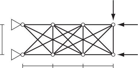
Consider the plane truss in Figure 1(a), where $L=1\,\mathrm{m}$. The truss consists of $m=19$ members and has $d=12$ degrees of freedom of the displacements. As for the constant external load (i.e., $\boldsymbol{p}_{\mathrm{d}}$ in (7)), a horizontal force of $50\,\mathrm{kN}$ is applied at each of the rightmost nodes. A vertical force of $10\lambda\,\mathrm{kN}$ is applied at the upper rightmost node as the proportionally increasing load (i.e., $\lambda\boldsymbol{p}_{\mathrm{r}}$ in (7)). The yield stress is $\sigma_{\mathrm{y}}=200\,\mathrm{MPa}$.

The initial point for Algorithm 1 is $\boldsymbol{x}_{0}=(1000,\dots,1000)^{\top}$ in $\mathrm{mm^{2}}$. The upper bound for the structural volume is given by $V=\boldsymbol{c}^{\top}\boldsymbol{x}_{0}=2.6430\times 10^{7}\,\mathrm{mm^{3}}$. The parameters for Algorithm 1 were chosen as $r=100\,\mathrm{mm^{2}}$, $r_{\min}=10^{-4}\,\mathrm{mm^{2}}$, $\epsilon=5\times 10^{-4}\,\mathrm{mm^{2}}$, $\rho=0.75$, $\eta=0.01$, $\beta=0.8$, $\tau_{\max}=50$, and $B_{0}$ is the identity matrix.

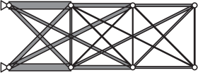
For $\alpha=1$, the solution obtained by Algorithm 1 is shown in Figure 2(a), where the width of each member is proportional to its cross-sectional area. The algorithm terminates after solving $376$ QP problems. The number of MILP problems solved for the objective function evaluations is $3699$. The obtained solution satisfies the termination condition $\|\boldsymbol{d}_{k}\|<\epsilon$ with a small value of the stencil radius, $r=4.2\times 10^{-3}\,\mathrm{mm^{2}}$. The worst-case limit load factor of the obtained solution is $14.4979$, while that of the initial design is $6.7187$. The worst-case scenarios for the obtained solution, as well as the corresponding collapse modes, are collected in Figure 3, where the damaged members are removed from the figures. It is emphasized that the limit load factors of these seven scenarios are all equal to the objective value, $14.4979$. In contrast, the worst-case scenario for the initial design is only the one shown in Figure 3(d). It seems to be natural that a local optimal solution of a redundancy optimization problem has multiple worst-case scenarios in general. Namely, multiplicity of worst-case scenarios means that, if we attempt to increase the limit load factor corresponding to a certain scenario, then the one corresponding to another scenario decreases.

(a)

(b)

(c)

(d)

(e)

(f)

(g)

(h)

(i)

Figure 4: The worst-case scenarios for the solution with $\alpha=2$ in example (I).

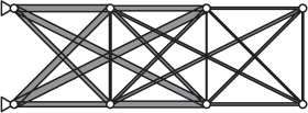
We next examine $\alpha=2$. The solution obtained by Algorithm 1 is shown in Figure 2(b). The algorithm terminates after solving $327$ QP problems and $3326$ MILP problems. The obtained solution satisfies the termination condition $\|\boldsymbol{d}_{k}\|<\epsilon$ with a small value of the stencil radius, $r=2.4\times 10^{-3}\,\mathrm{mm^{2}}$. The worst-case limit load factor of the obtained solution is $6.5509$, while that of the initial design is $3.0474$. Figure 4 collects the worst-case scenarios for the obtained solution. Namely, the multiplicity of the worst-case scenarios is $9$. In contrast, the worst-case scenario for the initial design is unique and is the one shown in Figure 4(d). It is worth noting that the objective function is not differentiable in general at a point having multiple worst-case scenarios. Nevertheless, the proposed algorithm could find a solution with large multiplicity.

The ground structure in Figure 1(a) becomes unstable if a particular set of three members is removed. This means that the redundancy optimization problem, (6), loses its meaning for $\alpha\geq 3$. This is because we assume that a damaged structural component is completely absent from the structure. In contrast, if we adopt a nonzero degree of damage, $\gamma$, as discussed in Remark 1, then problem (6) has meaning even for $\alpha\geq 3$.

When we set $\alpha=0$, structural degradation is not considered, and the redundancy optimization of the limit load factor reverts to the conventional limit design (the optimal plastic design). The optimal solution of the limit design problem, obtained by linear programming, is shown in Figure 1(b). It is worth noting that this is a statically determinate truss. Hence, the truss becomes unstable (kinematically indeterminate) if any single member is removed. Therefore, the truss has no redundancy; more precisely, the strong redundancy defined by [15] is equal to zero.

(a)

(b)

Figure 5: Example (II). 5(a) Problem setting; and 5(b) the optimal solution without considering redundancy (i.e., $\alpha=0$).

(a)

(b)

Figure 6: The solutions obtained in example (II). 6(a) $\alpha=1$; and 6(b) $\alpha=2$.

(a)

(b)

(c)

(d)

(e)

Figure 7: Some of the worst-case scenarios for the solution with $\alpha=1$ in example (II). The damage scenarios obtained by reflecting the scenarios in Figures 7(a), 7(b), 7(c), and 7(d) across the axis of symmetry are also the worst-case scenarios.

(a)

(b)

(c)

(d)

(e)

(f)

(g)

(h)

(i)

Figure 8: Some of the worst-case scenarios for the solution with $\alpha=2$ in example (II). The damage scenarios obtained by reflecting these scenarios across the axis of symmetry are also the worst-scenarios.

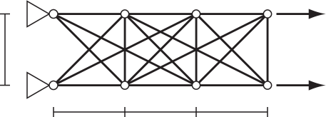
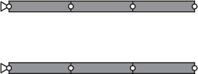
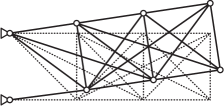
We next consider a different loading condition shown in Figure 5(a), where proportionally increasing forces of $50\lambda\,\mathrm{kN}$ are applied horizontally at the two rightmost nodes. The optimal solution of the classical limit design problem (i.e., $\alpha=0$) is apparently the one shown in Figure 5(b). Thus the optimal solution of the conventional optimization problem has no redundancy.

When we set $\alpha=1$, Algorithm 1 finds the solution shown in Figure 6(a). The algorithm terminates after solving $200$ QP problems and $1960$ MILP problems. At the final iteration, the stencil radius is $r=4.2\times 10^{-3}\,\mathrm{mm^{2}}$, and the solution satisfies the termination condition at step 3. The worst-case limit load factor of the obtained solution is $7.2812$, while that of the initial design is $5.7889$. At the obtained solution, the multiplicity of the worst-case scenarios is $9$. Among them, five scenarios are shown in Figure 7; namely, since the obtained solution has symmetry, the damage scenarios obtained by reflecting the ones in Figures 7(a), 7(b), 7(c), and 7(d) across the axis of symmetry are also the worst-case scenarios. The collapse mode in Figure 7(e) should be symmetric, if the obtained design is strictly symmetric. It is worth noting that we do not impose the constraints on symmetry of the design variables in the process of optimization. Asymmetry in Figure 7(e) is due to numerical errors in symmetry.

For $\alpha=2$, the solution obtained by Algorithm 1 is shown in Figure 6(b), where $378$ QP problems and $4014$ MILP problems are solved. The algorithm terminates at step 1, which means that the objective value at any sample point is not better than that at the obtained solution. It is worth noting that the limit load factors of many damage scenarios coincide at the obtained solution. Indeed, the multiplicity of the worst-case scenarios is $18$. Among them, $9$ scenarios are collected in Figure 8. Due to symmetry of the solution, the damage scenarios that are obtained by reflecting the ones in Figure 8 across the axis of symmetry are also the worst-case scenarios. The worst-case limit load factor of the obtained solution is $3.2773$, while that of the initial solution is $1.7889$.

In all the examples presented above, all the candidate members of the ground structure present in the obtained solution. Since the proposed algorithm is based upon the SQP method, it in principle allows some members to vanish. Since the global optimality of the obtained solution is not guaranteed, it is possible that the obtained solution is only a local optimal solution that is not globally optimal and some members vanish at a global optimal solution. Or, a global optimal solution may truly have all the members in the ground structure. This issue remains to be studied.

5 Summary and discussion

This paper has defined a concept of redundancy optimization of structures. Roughly speaking, the redundancy optimization maximizes the structural functionality in the worst-case scenario when deficient structural components are unknown a priori. The notion of redundancy is related to robustness against uncertainty in the set of deficient components. In accordance with this relation, the proposed redundancy optimization formulation is naturally consistent with a robust optimization of structures, in which one attempts to optimize the worst-case value of the objective function under uncertainty in structural environment.

A derivative-free optimization method has been proposed to solve the redundancy optimization problem. The method combines the SQP method and the finite-difference method with a varying difference increment. The numerical examples show that this algorithm can find a solution with multiple worst-case scenarios. Like a multiple eigenvalue in the eigenvalue optimization [23], a multiple limit load factor may not be differentiable. Hence, it is rather surprising that the proposed SQP-based algorithm can find a solution with large multiplicity of limit load factors. Fundamental properties, such as continuity and smoothness, of the worst-case limit load factor as a function of the member cross-sectional areas are not investigated yet. Hence, the optimality condition of the redundancy optimization problem considered in this paper also remains to be studied.

As a related design optimization problem, we may consider direct maximization of a quantitative measure of redundancy. For instance, the strong redundancy is defined by

$$\hat{\alpha}(\boldsymbol{x};h^{\mathrm{c}})=\max\{\alpha\mid h(\boldsymbol{s})\leq h^{\mathrm{c}}\ (\forall\boldsymbol{s}\in D(\boldsymbol{x};\alpha))\},$$

where $h^{\mathrm{c}}$ is the specified allowance of the structural performance [15]. Maximization of the strong redundancy is formulated as follows:

$$\displaystyle\mathop{\mathrm{Max.}} \displaystyle\hat{\alpha}(\boldsymbol{x};h^{\mathrm{c}})$$ (16a)

$$\mathop{\mathrm{s.{\,}t.}} \displaystyle\boldsymbol{x}\in X.$$ (16b)

Obviously, this problem is closely related to problem (6). Let $\boldsymbol{x}^{*}$ and $h^{*}$ denote the optimal solution and the optimal value of problem (6), respectively. If $h^{\mathrm{c}}\geq h^{*}$, then $\boldsymbol{x}^{*}$ satisfies $\hat{\alpha}(\boldsymbol{x}^{*};h^{\mathrm{c}})\geq\alpha$. Therefore, the optimal solution of problem (16) can be explored by solving problem (6) with varying the value of $\alpha$. Another possible formulation, that allows to handle several measures of structural performance, may be written as follows:

$$\displaystyle\mathop{\mathrm{Min.}} \displaystyle c(\boldsymbol{x})$$ (17a)

$$\mathop{\mathrm{s.{\,}t.}} \displaystyle h_{j}(\boldsymbol{s})\leq h^{\mathrm{c}}_{j}\ (\forall\boldsymbol{s}\in D(\boldsymbol{x};\alpha)),\quad j=1,\dots,k,$$ (17b)

$$\displaystyle\boldsymbol{x}\in X.$$ (17c)

Here, $c(\boldsymbol{x})$ is the cost function such as the structural volume. This optimization problem is consistent with the general methodology of robust optimization [2]. Also, problem (17) with $\alpha=1$ is essentially similar to the fail-safe optimization problem of structures studied in Sun et al. [25] and Nguyen and Arora [20].

This paper has developed a generic framework for optimizing structures with guaranteeing the magnitude of redundancy. Other concepts of redundancy optimization based on different definitions of redundancy may be formulated. Although attention of this paper has been focused on truss structures, the presented concept can be applied to frame structures in a straightforward manner. Also, structural performance other than the limit load factor, such as the compliance and the violation of the displacement constraints, can be considered within the presented framework. The proposed algorithm might probably have many possibilities of improvements and extensions. Especially, improvements from the viewpoints of computational cost and convergence property may remain to be studied. Also, extension to nonlinear constraints could be explored. Moreover, in the presented numerical examples, all the solutions have all the members in the ground structure, although an SQP method generally allows some members to vanish if such a solution is optimal. It remains to be studied if the obtained solution is only a local optimal solution and some members vanish at a global optimal solution, or, a global optimal solution truly has all the members in the ground structure.

References

- Ben-Haim [2006] Ben-Haim, Y. (2006). Information-gap decision theory: Decisions under severe Uncertainty (2nd ed.), Academic Press, London.
- Ben-Tal et al. [2009] Ben-Tal, A., El Ghaoui, L., and Nemirovski, A. (2009). Robust optimization, Princeton University Press, Princeton.
- Ben-Tal and Nemirovski [1997] Ben-Tal, A., and Nemirovski, A. (1997). “Robust truss topology design via semidefinite programming.” SIAM Journal on Optimization, 7, 991–1016.
- Bertero and Bertero [1999] Bertero, R. D., and Bertero, V. V. (1999). “Redundancy in earthquake-resistant design.” Journal of Structural Engineering (ASCE), 125, 81–88.
- Brett and Lu [2000] Brett, C., and Lu, Y. (2013). “Assessment of robustness of structures: current state of research.” Frontiers of Structural and Civil Engineering, 7, 356–368.
- Cherkaev and Cherkaev [2003] Cherkaev, E., and Cherkaev, A. (2003). “Principal compliance and robust optimal design.” Journal of Elasticity, 72, 71–98.
- Conn et al. [2009] Conn, A. R., Scheinberg, K., and Vincente, L. N. (2009). Introduction to derivative-free optimization, SIAM, Philadelphia.
- Frangopol and Curley [1987] Frangopol, D. M., and Curley, J. P. (1987). “Effects of damage and redundancy on structural reliability.” Journal of Structural Engineering (ASCE), 113, 1533–1549.
- Guo et al. [2013] Guo, X., Zhang, W., and Zhang, L. (2013). “Robust structural topology optimization considering boundary uncertainties.” Computer Methods in Applied Mechanics and Engineering, 253, 356–368.
- Hashimoto and Kanno [2015] Hashimoto, D., Kanno, Y. (2015). “A semidefinite programming approach to robust truss topology optimization under uncertainty in locations of nodes.” Structural and Multidisciplinary Optimization, 51, 439–461.
- IBM ILOG [2015] IBM ILOG. (2015). User’s manual for CPLEX, http://www.ilog.com (Accessed August 2015).
- Jang et al. [2011] Jang, G.-W., van Dijk, N. P., and van Keulen, F. (2012). “Topology optimization of MEMS considering etching uncertainties using the level-set method.” International Journal for Numerical Methods in Engineering, 92, 571–588.
- Jansen et al. [2014] Jansen, M., Lombaert, G., Schevenels, M., and Sigmund, O. (2014). “Topology optimization of fail-safe structures using a simplified local damage model.” Structural and Multidisciplinary Optimization, 49, 657–666.
- Kanno [2012] Kanno, Y. (2012). “Worst scenario detection in limit analysis of trusses against deficiency of structural components.” Engineering Structures, 42, 33–42.
- Kanno and Ben-Haim [2011] Kanno, Y., and Ben-Haim, Y. (2011). “Redundancy and robustness, or, when is redundancy redundant?” Journal of Structural Engineering (ASCE), 137, 935–945.
- Kelley [2011] Kelley, C. T. (2011). Implicit filtering, SIAM, Philadelphia.
- Kobayashi et al. [2016] Kobayashi, Y., Higashikawa, Y., Katoh, N., and Sljoka, A. (2016). “Characterizing redundant rigidity and redundant global rigidity of body-hinge graphs.” Information Processing Letters, 116, 175–178.
- Mohr et al. [2014] Mohr, D. P., Stein, I., Matzies, T., and Knapek, C. A. (2014). “Redundant robust topology optimization of truss.” Optimization and Engineering, 15, 945–972.
- Mousavi and Gardoni [2014] Mousavi, M. E., Gardoni, P. (2014). “Integrity index and integrity-based optimal design of structural systems.” Engineering Structures, 60, 206–213.
- Nguyen and Arora [1982] Nguyen, D. T., and Arora, J. S. (1982). “Fail-safe optimal design of complex structures with substructures.” Journal of Mechanical Design (ASME), 104, 861–868.
- Nocedal and Wright [2006] Nocedal, J., and Wright, S. J. (2006). Numerical optimization (2nd ed.), Springer, New York.
- Schafer and Bajpai [2005] Schafer, B. W., and Bajpai, P. (2005). “Stability degradation and redundancy in damaged structures.” Engineering Structures, 27, 1642–1651.
- Seyranian et al. [1994] Seyranian, A. P., Lund, E., and Olhoff, N. (1994). “Multiple eigenvalues in structural optimization problem.” Structural Optimization, 8, 207–227.
- Sigmund [2009] Sigmund, O. (2009). “Manufacturing tolerant topology optimization.” Acta Mechanica Sinica, 25, 227–239.
- Sun et al. [1976] Sun, P. F., Arora, J. S., and Haug Jr., E. J. (1976). “Fail-safe optimal design of structures.” Engineering Optimization, 2, 43–53.
- Takezawa et al. [2011] Takezawa, A., Nii, S., Kitamura, M., and Kogiso, N. (2011). “Topology optimization for worst load conditions based on the eigenvalue analysis of an aggregated linear system.” Computer Methods in Applied Mechanics and Engineering, 200, 2268–2281.
- Tangaramvong et al. [2013] Tangaramvong, S., Tin-Loi, F., Wu, D., and Gao, W. (2013). “Mathematical programming approaches for obtaining sharp collapse load bounds in interval limit analysis.” Computers and Structures, 125, 114–126.
- The MathWorks, Inc. [2015] The MathWorks, Inc.. (2015). MATLAB documentation, http://www.mathworks.com (Accessed December 2015).
- Yonekura and Kanno [2010] Yonekura, K., and Kanno, Y. (2010). “Global optimization of robust truss topology via mixed integer semidefinite programming.” Optimization and Engineering, 11, 355–379.
- Zhu and Frangopol [2012] Zhu, B., and Frangopol, D. M. (2012). “Reliability, redundancy and risk as performance indicators of structural systems during their life-cycle.” Engineering Structures, 41, 34–49.
- Žiha [2000] Žiha, K. (2000). “Redundancy and robustness of systems of events.” Probabilistic Engineering Mechanics, 15, 347–357.