Anatomy of double heavy-quark initiated processes

Abstract

A number of phenomenologically relevant processes at hadron colliders, such as Higgs and $Z$ boson production in association with $b$ quarks, can be conveniently described as scattering of heavy quarks in the initial state. We present a detailed analysis of this class of processes, identifying the form of the leading initial-state collinear logarithms that allow the relation of calculations performed in different flavour schemes in a simple and reliable way. This procedure makes it possible to assess the size of the logarithmically enhanced terms and the effects of their resummation via heavy-quark parton distribution functions. As an application, we compare the production of (SM-like and heavy) scalar and vector bosons in association with $b$ quarks at the LHC in the four- and five-flavour schemes as well as the production of a heavy $Z^{\prime}$ in association with top quarks at a future 100 TeV hadron collider in the five- and six-flavour schemes. We find that, in agreement with a previous analysis of single heavy-quark initiated processes, the size of the initial-state logarithms is mitigated by a kinematical suppression. The most important effects of the resummation are a shift of the central predictions typically of about 20% at a justified value of the scale of each considered process and a significant reduction of scale variation uncertainties.

1 Introduction

With the imminent restart of data-taking at LHC Run II the need for accurate theoretical predictions for energetic final states, typically involving the production of heaviest particles of the Standard Model (SM), becomes more and more pressing. The study of associated production of (possibly new) vector or scalar bosons in association with heavy quarks, such as top and bottom quarks, are among the highest priorities of the new run. In particular, $b$ quarks play an important role in the quest for new physics as well as for precise SM measurements from both an experimental and a theoretical perspective. Firstly, they provide a very clean signature as they may easily be identified in a detector due to the displacement of vertices with respect to the collision point, a consequence of the $b$-quark long lifetime. Secondly, the relative strength of the Higgs Yukawa coupling (or possibly of new scalar states) to the heavy quarks is important in determining the phenomenology, both in production as well as in decay. In particular, production associated with $b$ quarks could provide the leading mode for Higgs bosons with enhanced Yukawa couplings in many scenarios beyond the Standard Model.

At hadron colliders, any process that features heavy quarks can be described according to two different and complementary approaches. In the massive or four-flavor (4F) scheme (in the case of $b$ quarks), the heavy quark is produced in the hard scattering and arises as a massive particle in the final state. The dependence on the heavy quark mass $m_{b}$ is retained in the matrix element and explicit logarithms of $Q/m_{b}$, $Q$ being some hard scale of the process, appear at each order in perturbation theory as a result of collinearly enhanced (yet finite) splittings $q\to qg$ or of a gluon into heavy quark pairs, $g\to q\bar{q}$. On the other hand, in the massless or five-flavour (5F) scheme (in the case of $b$ quarks), $Q\gg m_{b}$ is assumed and the heavy quark is treated on the same footing as the light quarks: it contributes to the proton wave function and enters the running of the strong coupling constant $\alpha_{s}$. In this scheme the heavy quark mass is neglected in the matrix element and the collinear logarithms that may spoil the convergence of the perturbative expansion of the 4F scheme cross section are resummed to all orders in the evolution of the heavy quark parton density.

In a previous work Maltoni:2012pa , we examined processes involving a single $b$ quark in both lepton-hadron and hadron-hadron collisions. It was found that, at the LHC, unless a very heavy particle is produced in the final state, the effects of initial-state collinear logarithms are always modest and such logarithms do not spoil the convergence of perturbation theory in 4F scheme calculations. This behaviour was explained by two main reasons, one of dynamical and the other of kinematical nature. The first is that the effects of the resummation of the initial-state collinear logarithms is relevant mainly at large Bjorken-$x$ and in general keeping only the explicit logs appearing at NLO is a very good approximation. The second reason is that the naïve scale $Q$ that appears in the collinear logarithms turns out to be suppressed by universal phase space factors that, at hadron colliders, reduce the size of the logarithms for processes taking place. As a result, a consistent and quantitative analysis of many processes involving one $b$ quark in the initial state was performed and a substantial agreement between total cross sections obtained at NLO (and beyond) in the two schemes found within the expected uncertainties.

In this work we focus on processes that can be described by two $b$ quarks in the initial state, such as $pp\to Hb\bar{b}$ or $pp\to Zb\bar{b}$. As already sketched in  Maltoni:2012pa , the same arguments used for single heavy-quark initiated processes can be used to analyse the double heavy-quark case. One may naïvely expect that the resummation effects for processes with two $b$ quarks in the initial state can be simply obtained by “squaring”, in some sense, those of processes with only one $b$ quark. There are, however, a number of features that are particular to the double heavy-quark processes and call for a dedicated work. One is that the lowest order contribution in the 4F scheme appears for the first time among the NNLO real corrections to the leading order 5F scheme calculation. Furthermore, due to the simplicity of the 5F description (i.e. Born amplitudes are $2\to 1$ processes), results in the 5F scheme are now available at NNLO, while, thanks to the progress in the automation of NLO computations, 4F scheme results have become easily accessible for a wide range of final states. In fact, it is easy to understand that a meaningful comparison between the two schemes for double heavy-quark initiated processes starts to be accurate if results are taken at NNLO for the 5F and at NLO for the 4F case.

Both $pp\to Hb\bar{b}$ or $pp\to Zb\bar{b}$ have been considered in previous works. For the LHC, it was demonstrated that consistent results for both the total cross section and differential distributions for bottom-fusion initiated Higgs production can be obtained in both schemes Dawson:2003kb ; Maltoni:2003pn ; Campbell:2004pu ; Harlander:2011aa ; Wiesemann:2014ioa . Analogous studies were performed for bottom-fusion initiated $Z$ production Campbell:2000bg ; Maltoni:2003pn ; FebresCordero:2008ci ; Cordero:2009kv ; Frederix:2011qg . All these studies suggested that the appropriate factorisation and renormalisation scales associated to these processes are to be chosen smaller than the mass of the final state heavy particles. In particular, scales of about $M_{H,Z}/4$ have been proposed in order to stabilise the perturbative series and make the four- and five-flavor predictions closer other. $(M_{H}+2m_{b})/4$ is the scale adopted by the LHC Higgs Cross Section Working Group (HXSWG) to match the NLO 4F and NNLO 5F scheme predictions in case of bottom-fusion initiated Higgs production via the Santander interpolation Harlander:2011aa and via the use of consistently matched calculations Bonvini:2015pxa ; Forte:2015hba ; Bonvini:2016fgf .

While previous studies support a posteriori the evidence that smaller scales make the four- and five-flavor pictures more consistent, no complete analysis of the relation of the two schemes in the case of double heavy-quark initiated processes has been provided. In particular, no analytic study of the collinear enhancement of the cross section and the kinematics of this class of processes has been performed.

In this work, we fill this gap by extending our previous work to double heavy-quark production. We first present an analytic comparison of the two schemes that allow us to unveil a clear relation between them, establish the form of the logarithmic enhancements and determine their size. We then compare the predictions for LHC phenomenology in a number of relevant cases focusing on LHC Run II. Furthermore, we expand our investigation to high energy processes involving top quarks at future colliders. At centre-of-mass energies of order $100$ TeV, a new territory far beyond the reach of the LHC would be explored. At such an energy, much heavier particles could be produced at colliders and top-quark PDFs may become of relevance in processes involving top quarks in the initial state.

The structure of the work is as follows. In Sect. 2 we examine the kinematics of 2 to 3 body scattering and calculate the phase space factor for the particular case of $b$-initiated Higgs production—we thus derive the logarithmic contributions to the cross section which arise in a 4F scheme. We then proceed to generate kinematic distributions for the processes and use these to analyse the 4F and 5F scheme results. We conclude the section by suggesting a factorisation scale at which results from either process may be meaningfully compared. In Sect. 3 we compare the results on total cross sections obtained in both schemes for a number of phenomenologically relevant processes at the LHC and future colliders. Finally, our conclusions are presented in Sect. 4.

2 Different heavy quark schemes: analytical comparison

We start by considering Higgs boson production via $b\bar{b}$ fusion in the 4F scheme. The relevant partonic subprocess is

$$g(p_{1})+g(p_{2})\to b(k_{1})+H(k)+\bar{b}(k_{2}),$$ (1)

where the $b$ quarks in the final state are treated as massive objects. Since the $b$-quark mass $m_{b}$ is much smaller than the Higgs boson mass $M_{H}$, we expect the cross section for the process (1) to be dominated by the configurations in which the two final-state $b$ quarks are emitted collinearly with the incident gluons. Indeed the quark-antiquark channel ($q\bar{q}\to b\bar{b}H$) that also contributes to the leading-order cross section in the 4F scheme is very much suppressed with respect to the gluon-gluon one. In order to estimate the importance of large transverse momentum $b$ quarks in the gg channel, as compared to the dominant collinear configurations, we will perform an approximate calculation of the cross section for the process (1) limiting ourselves to the dominant terms as $m_{b}\to 0$. The result will then be compared to the full leading-order 4F scheme calculation. We present here the final result; the details of the calculation can be found in Appendix A.

The differential partonic cross section can be expressed as a function of five independent invariants, which we choose to be

$$\hat{s}=(p_{1}+p_{2})^{2};\quad t_{1}=(p_{1}-k_{1})^{2};\quad t_{2}=(p_{2}-k_{2})^{2};\quad s_{1}=(k_{1}+k)^{2};\quad s_{2}=(k_{2}+k)^{2}.$$ (2)

Collinear singularities appear, for $m_{b}^{2}=0$, either when

$$t_{1}\to 0;\qquad t_{2}\to 0,$$ (3)

or when

$$u_{1}\to 0;\qquad u_{2}\to 0,$$ (4)

where

$$u_{1}=(p_{1}-k_{2})^{2};\qquad u_{2}=(p_{2}-k_{1})^{2}.$$ (5)

The configuration in Eq. (3) is achieved for

$$k_{1}=(1-z_{1})p_{1};\qquad k_{2}=(1-z_{2})p_{2};\qquad 0\leq z_{i}\leq 1$$ (6)

while the one in Eq. (4) corresponds to

$$k_{1}=(1-z_{1})p_{2};\qquad k_{2}=(1-z_{2})p_{1}.$$ (7)

In both cases we find

$$\hat{s}=\frac{M_{H}^{2}}{z_{1}z_{2}};\qquad s_{1}=\frac{M_{H}^{2}}{z_{1}};\qquad s_{2}=\frac{M_{H}^{2}}{z_{2}}.$$ (8)

An explicit calculation yields

$$\hat{\sigma}^{\rm 4F,coll}(\hat{\tau})=\hat{\tau}\frac{\alpha_{s}^{2}}{4\pi^{2}}\frac{G_{F}\pi}{3\sqrt{2}}\frac{m_{b}^{2}}{M_{H}^{2}}2\int_{0}^{1}dz_{1}\int_{0}^{1}dz_{2}\,P_{qg}(z_{1})P_{qg}(z_{2})L(z_{1},\hat{\tau})L(z_{2},\hat{\tau})\delta\left(z_{1}z_{2}-\hat{\tau}\right),$$ (9)

where

$$\hat{\tau}=\frac{M_{H}^{2}}{\hat{s}},$$ (10)

$P_{qg}(z)$ is the leading-order quark-gluon Altarelli-Parisi splitting function

$$P_{qg}(z)=\frac{1}{2}[z^{2}+(1-z)^{2}],$$ (11)

and

$$L(z,\hat{\tau})=\log\left[\frac{M_{H}^{2}}{m_{b}^{2}}\frac{(1-z)^{2}}{\hat{\tau}}\right].$$ (12)

The suffix “coll” reminds us that we are neglecting less singular contributions as $m_{b}\to 0$, i.e. either terms with only one collinear emission, which diverge as $\log m_{b}^{2}$, or terms which are regular as $m_{b}\to 0$.

We now observe that the leading-order partonic cross section for the process

$$b(q_{1})+\bar{b}(q_{2})\to H(k),$$ (13)

relevant for calculations in the 5F scheme, is given by stirling

$$\hat{\sigma}^{\rm 5F}(\hat{\tau})=\frac{G_{F}\pi}{3\sqrt{2}}\frac{m_{b}^{2}}{M_{H}^{2}}\delta(1-\hat{\tau}),$$ (14)

with

$$\hat{s}=(q_{1}+q_{2})^{2}.$$ (15)

Hence, the 4F scheme cross section in the collinear limit, Eq. (9), can be rewritten as

$$\hat{\sigma}^{\rm 4F,coll}(\hat{\tau})=2\int_{\hat{\tau}}^{1}dz_{1}\int_{\frac{\hat{\tau}}{z_{1}}}^{1}dz_{2}\,\left[\frac{\alpha_{s}}{2\pi}P_{qg}(z_{1})L(z_{1},\hat{\tau})\right]\left[\frac{\alpha_{s}}{2\pi}P_{qg}(z_{2})L(z_{2},\hat{\tau})\right]\hat{\sigma}^{\rm 5F}\left(\frac{\hat{\tau}}{z_{1}z_{2}}\right).$$ (16)

The physical interpretation of the result Eq. (16) is straightforward: in the limit of collinear emission, the cross section for the parton process (1) is simply the $b\bar{b}\to H$ cross section convolved with the probability that the incident gluons split in a $b\bar{b}$ pair. This probability is logarithmically divergent as $m_{b}\to 0$, and this is the origin of the two factors of $L(z_{i},\hat{\tau})$.

The arguments of the two collinear logarithms exhibit a dependence on the momentum fractions $z_{1},z_{2}$, Eq. (12). This dependence is subleading in the collinear limit $m_{b}\to 0$ and indeed it could be neglected in this approximation; however, the class of subleading terms induced by the factor $(1-z_{i})^{2}/\hat{\tau}$ in Eq. (12) is of kinematical origin (it arises from the integration bounds on $t_{1}$ and $t_{2}$, as shown in Appendix A) and therefore universal in some sense, as illustrated in Ref. Maltoni:2012pa . We also note that the arguments of the two collinear logs depend on both $z_{1}$ and $z_{2}$; this is to be expected, because the integration bounds on $t_{1}$ and $t_{2}$ are related to each other. However, in some cases (for example, if one wants to relate the scale choice to a change of factorisation scheme, as in ef. Maltoni:2007tc ) a scale choice which only depends on the kinematics of each emitting line might be desirable. We have checked that the replacement

$$\log\left[\frac{M_{H}^{2}}{m_{b}^{2}}\frac{(1-z_{i})^{2}}{z_{1}z_{2}}\right]\to\log\left[\frac{M_{H}^{2}}{m_{b}^{2}}\frac{(1-z_{i})^{2}}{z_{i}}\right]$$ (17)

has a moderate effect on physical cross sections. The replacement would make the scale at which the four- and five-flavor scheme results are comparable lower by about 20/30% but does not qualtatively modify our arguments and results below.

The corresponding 4F scheme physical cross section in hadron collisions at centre-of-mass energy $\sqrt{s}$ is given by

$$\sigma^{\rm 4F,coll}(\tau)=\int_{\tau}^{1}dx_{1}\,\int_{\frac{\tau}{x_{1}}}^{1}dx_{2}\,g(x_{1},\mu_{F}^{2})g(x_{2},\mu_{F}^{2})\hat{\sigma}^{\rm 4F,coll}\left(\frac{\tau}{x_{1}x_{2}}\right),$$ (18)

where $g(x,\mu_{F}^{2})$ is the gluon distributon function, $\mu_{F}$ is the factorisation scale, and

$$\tau=\frac{M_{H}^{2}}{s}.$$ (19)

After some (standard) manipulations, we get

$$\sigma^{\rm 4F,coll}(\tau)=2\int_{\tau}^{1}dx_{1}\,\int_{\frac{\tau}{x_{1}}}^{1}dx_{2}\,\hat{\sigma}^{\rm 5F}\left(\frac{\tau}{x_{1}x_{2}}\right)$$

$$\quad\int^{1}_{x_{1}}\frac{dz_{1}}{z_{1}}\,\left[\frac{\alpha_{s}}{2\pi}P_{qg}(z_{1})L\left(z_{1},z_{1}z_{2}\right)\right]g\left(\frac{x_{1}}{z_{1}},\mu_{F}^{2}\right)\int^{1}_{x_{2}}\frac{dz_{2}}{z_{2}}\,\left[\frac{\alpha_{s}}{2\pi}P_{qg}(z_{2})L\left(z_{2},z_{1}z_{2}\right)\right]g\left(\frac{x_{2}}{z_{2}},\mu_{F}^{2}\right).$$ (20)

We are now ready to assess the accuracy of the collinear approximation in the 4F scheme. We first consider the total cross section. In table 1 we display the total 4F scheme cross section for the production of a Higgs boson at LHC 13 TeV for two values of the Higgs mass, namely $M_{H}=125$ GeV and $M_{H}=400$ GeV.

$M_{H}$	exact	collinear ME	collinear ME and PS
125 GeV	4.71 $\cdot\,10^{-1}$ pb	5.15 $\cdot\,10^{-1}$ pb	5.82 $\cdot\,10^{-1}$ pb
400 GeV	5.42 $\cdot\,10^{-3}$ pb	5.58 $\cdot\,10^{-3}$ pb	5.91 $\cdot\,10^{-3}$ pb

Table 1: Total cross sections for Higgs boson production at the LHC 13 TeV in the 4F scheme.

In the first column we give the exact leading order result; the second column contains the cross section with the squared amplitude approximated by its collinear limit, but the exact expression of the phase space measure. Finally, in the third column we give the results obtained with both the amplitude and the phase-space measure in the collinear limit, which corresponds to the expression in Eq. (20). From table 1 we conclude that the production of large transverse momentum $b$ quarks, correctly taken into account in the 4F scheme, amounts to an effect of order 20% on the total cross section and tends to decrease with increasing Higgs mass.

We now turn to an assessment of the numerical relevance of the subleading terms included by the definition Eq. (12) of the collinear logarithms. To this purpose we study the distribution of $(1-z_{1})^{2}/(z_{1}z_{2})$, which is the suppression factor of $M_{H}^{2}/m_{b}^{2}$ in the arguments of the logs. The results are displayed in Fig. 1 for Higgs production at the LHC at 13 TeV and for two different values of the Higgs boson mass.

Figure 1: Normalised distribution (events/bin) of $(1-z_{1})^{2}/\hat{\tau}$ for $b$-initiated Higgs production in $pp$ collisions at LHC 13 TeV for $M_{H}=125$ GeV (left) and $M_{H}=400$ GeV (right). Both $\mu_{R}$ and $\mu_{F}$ are set to $M_{H}$. The vertical lines represent the values below which 68% and 90% of events lie.

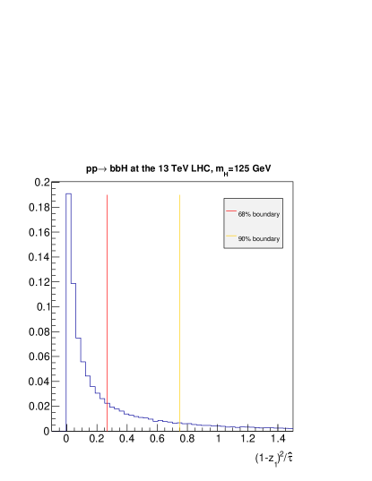
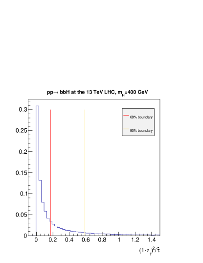
The two distributions behave in a similar way: both are strongly peaked around values smaller than 1; in particular, the 68% threshold is in both cases around $0.2$. This confirms that, altough formally subleading with respect to $\log\frac{M_{H}^{2}}{m_{b}^{2}}$, in practice the terms proportional to $\log\frac{(1-z_{i})^{2}}{z_{1}z_{2}}$ give a sizeable contribution to the total cross section.

A further confirmation is provided by the distributions in Fig. 2, where the full cross sections, together with their collinear and double-collinear approximations, are plotted as functions of the partonic centre-of-mass energy.

Figure 2: Distribution of the 4F scheme cross section as a function of the partonic centre-of-mass energy $\hat{s}$ for a Higgs of mass 125 GeV (above) and of mass 400 GeV (below). The solid line represents the full cross section at leading-order, while the dashed line represents the collinear limit.

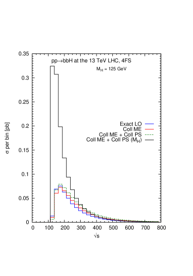
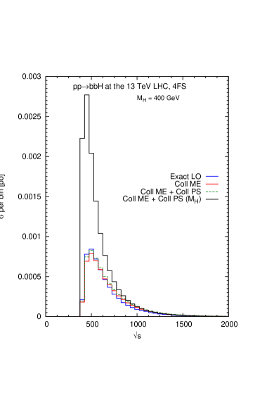
We see that the collinear cross section provides a good approximation to the full 4F scheme result. In the same picture we show the collinear cross section with the factors of $L(z_{i},z_{1}z_{2})$ replaced by $\log\frac{M_{H}^{2}}{m_{b}^{2}}$ (solid black histogram). It is clear that in this case the collinear cross section substantially differs from the exact result.

We now consider the 5F scheme, where the $b$ quark is treated as a massless parton and collinear logarithms are resummed to all orders by the perturbative evolution of the parton distribution function. Eq. (14) leads to a physical cross section

$$\sigma^{\rm 5F}(\tau)=2\int_{\tau}^{1}dx_{1}\,b(x_{1},\mu_{F}^{2})\int_{\frac{\tau}{x_{1}}}^{1}dx_{2}\,b(x_{2},\mu_{F}^{2})\hat{\sigma}^{\rm 5F}\left(\frac{\tau}{x_{1}x_{2}}\right).$$ (21)

In order to make contact with the 4F scheme calculation, we observe that the $b$ quark PDF can be expanded to first order in $\alpha_{s}$:

$$b(x,\mu_{F}^{2})=\frac{\alpha_{s}}{2\pi}L_{b}\int^{1}_{x}\frac{dy}{y}\,P_{qg}(y)g\left(\frac{x}{y},\mu_{F}^{2}\right)+{\cal O}(\alpha_{s}^{2})=\tilde{b}^{(1)}(x,\mu_{F}^{2})+{\cal O}(\alpha_{s}^{2}),$$ (22)

where

$$L_{b}=\log\frac{\mu_{F}^{2}}{m_{b}^{2}}.$$ (23)

Correspondingly, we may define a truncated 5F cross section $\sigma^{\rm 5F,(1)}(\tau)$ which contains only one power of $\log m_{b}^{2}$ for each colliding $b$ quark. This is obtained by replacing Eq. (22) in Eq. (21) and performing the same manipulations that led us to Eq. (20): we get

$$\sigma^{\rm 5F,(1)}(\tau) =2\int_{\tau}^{1}dx_{1}\,\int_{\frac{\tau}{x_{1}}}^{1}dx_{2}\,\hat{\sigma}^{5F}\left(\frac{\tau}{x_{1}x_{2}}\right)$$

$$\int^{1}_{x_{1}}\frac{dy}{y}\,\left[\frac{\alpha_{s}}{2\pi}P_{qg}(y)L_{b}\right]g\left(\frac{x_{1}}{y},\mu_{F}^{2}\right)\int^{1}_{x_{2}}\frac{dz}{z}\,\left[\frac{\alpha_{s}}{2\pi}P_{qg}(z)L_{b}\right]g\left(\frac{x_{2}}{z},\mu_{F}^{2}\right).$$ (24)

Eq. (24) has exactly the same structure as the 4F scheme result in the collinear approximation Eq. (20), except that the collinear logarithms have a constant argument. Hence, it corresponds to the solid black curve in Fig. 2. We are therefore led to suggest that the 5F scheme results be used with a scale choice dictated by the above results, similar to what we have illustrated in Ref. Maltoni:2007tc . Such a scale is defined so that the two schemes give the same result:

$$\sigma^{\rm 5F,(1)}(\tau)=\sigma^{\rm 4F,coll}(\tau).$$ (25)

The explicit expression of $\tilde{\mu}_{F}$ is simply obtained by equating $\sigma^{\rm 5F,(1)}(\tau)$, Eq. (24), which is proportional to $L_{b}^{2}=\log^{2}\frac{\mu_{F}^{2}}{m^{2}}$, and $\sigma^{\rm 4F,coll}(\tau)$, Eq. (20), and solving for $L_{b}^{2}$. The residual dependence on $\mu_{F}$ due to the gluon parton density is suppressed by an extra power of $\alpha_{s}$ and can therefore be neglected; we adopt the standard choice $\mu_{F}=M$, with $M$ either the Higgs mass or the $Z^{\prime}$ mass. The size of the logarithmic terms kept explicitly in the 4F case is determined by arguments of the form $\frac{(1-z_{i})^{2}}{\hat{\tau}}$. For $\sqrt{s}=13$ GeV, and $m_{b}=4.75$ GeV, we find the following values for $\tilde{\mu}_{F}$:

$$b\bar{b}H,M_{H}=125\,{\rm GeV}:\qquad\qquad \tilde{\mu}_{F}\approx 0.36\,M_{H}$$

$$b\bar{b}Z^{\prime},M_{Z^{\prime}}=91.2\,{\rm GeV}:\qquad\qquad \tilde{\mu}_{F}\approx 0.38\,M_{Z^{\prime}}$$

$$b\bar{b}Z^{\prime},M_{Z^{\prime}}=400\,{\rm GeV}:\qquad\qquad \tilde{\mu}_{F}\approx 0.29\,M_{Z^{\prime}},$$ (26)

while for $\sqrt{s}=100$ TeV and $m_{t}=173.1$ GeV, we find

$$t\bar{t}Z^{\prime},M_{Z^{\prime}}=1\,{\rm TeV}:\qquad \tilde{\mu}_{F}\approx 0.40\,M_{Z^{\prime}}$$

$$t\bar{t}Z^{\prime},M_{Z^{\prime}}=5\,{\rm TeV}:\qquad \tilde{\mu}_{F}\approx 0.21\,M_{Z^{\prime}}$$

$$t\bar{t}Z^{\prime},M_{Z^{\prime}}=10\,{\rm TeV}:\qquad \tilde{\mu}_{F}\approx 0.16\,M_{Z^{\prime}}.$$ (27)

In both cases we have used the NNPDF30_lo_as_0130 PDF set Ball:2014uwa , with the appropriate number of light flavors. We have explicitly checked that the choice of $\mu_{F}=M_{H}/4$ for the gluon PDF and for the strong coupling constant does not modify in any significant way the value of $\tilde{\mu}_{F}$ that we obtain. This is expected given that the gluon-gluon luminosity and the dependence on $\alpha_{s}$ tend to compensate between numerator and denominator. We have also checked that, after the replacement in Eq. (17), the values of $\tilde{\mu}_{F}$ are typically about 20-30% smaller.

We note that the scale $\tilde{\mu}_{F}$ is in general remarkably smaller than the mass of the produced heavy particle. As in the case of single collinear logarithm, the reduction is more pronounced for larger values of the mass of the heavy particle compared to the available hadronic centre-of-mass energy. The above results suggest that a “fair” comparison between calculations in the two schemes should be performed at factorisation/renormalisation scales smaller than the naïve choice $\mu_{F}=M_{H}$. This evidence backs up the conclusions drawn in previous studies Maltoni:2003pn , although perhaps with a slightly larger value in the case of Higgs boson, $\tilde{\mu}\approx M_{H}/3$ rather than $M_{H}/4$.

The argument given above identifies a suitable choice for the factorisation/renormalisation scales such that, at the Born level and without resummation, the size of the logarithmic terms is correctly matched in the two schemes. At this point, further differences between the schemes can arise from the collinear resummation as achieved in the 5F scheme and from mass (power-like) terms which are present in the 4F scheme and not in the 5F one. Closely following the arguments of Ref. Maltoni:2003pn , to which we refer the interested reader for more details, we now numerically quantify the effect of the resummation. A careful study of the impact of power-like terms can be found in Refs. Forte:2015hba ; Bonvini:2015pxa ; Bonvini:2016fgf . These terms have been found to have an impact no stronger than a few percents.

Starting from Eq. (22), one can assess the accuracy of the ${\cal O}(\alpha_{s}^{1})$ (${\cal O}(\alpha_{s}^{2})$) approximations compared to the full $b(x,\mu^{2})$ resummed expression. The expansion truncated at order $\alpha_{s}^{p}$, often referred to as $\tilde{b}^{(p)}(x,\mu^{2})$ in the literature, does not feature the full resummation of collinear logarithms, but rather it contains powers $n$ of the collinear log with $1\leq n\leq p$.

In Fig. 3 we display the ratio $\frac{\tilde{b}^{(p)}(x,\mu^{2})}{b(x,\mu^{2})}$ for $p=1,2$ (using the same set of PDFs adopted throughout this work) as a function of the scale $\mu^{2}$ for various values of the momentum fraction $x$. Deviations from one of these curves are an indication of the size of terms of order ${\cal O}(\alpha_{s}^{p+1})$ and higher, which are resummed in the QCD evolution of the bottom quark PDFs.

Figure 3: The ratio $\tilde{b}^{(p)}/b$ for $p=1$ (left) and $p=2$ (right) as a function of the scale $\mu$ for for different values of $x$. The $n_{f}=4$ and $n_{f}=5$ sets of the NNPDF3.0 family (with $\alpha_{s}(M_{Z})=0.118$) are associated to the $\tilde{b}$ and $b$ computations respectively.

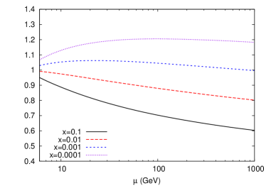
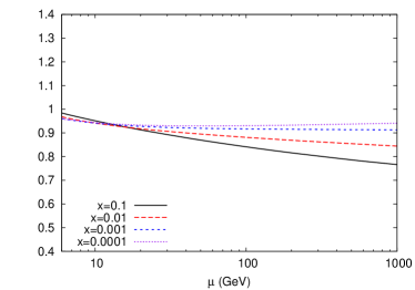
As observed in our previous work, at LO higher-order logarithms are important and $\tilde{b}^{(1)}(x,\mu^{2})$ is a poor approximation of the fully resummed distribution function. In particular, it overestimates the leading-log evolution of the $b$ PDF by 20% at very small $x$ and it underestimates it up to 30% at intermediate values of $x$. On the other hand, at NLO the explicit collinear logs present in a NLO 4F scheme calculation provide a rather accurate approximation of the whole resummed result at NLL; significant effects, of order up to 20%, appear predominantly at large values of $x$.

A similar behaviour characterises the top-quark PDFs. In Fig. 4 the ratio between the truncated top-quark PDFs $\tilde{t}$ and the evolved PDFs $t(x,\mu^{2})$ is displayed for four different values of $x$ and varying the factorization scale $\mu$.

Figure 4: Ratio $\tilde{t}/t$ at LO (left) and NLO (right) for several values of $x$ as a function of the scale $\mu$. The $n_{f}=5$ and $n_{f}=6$ sets of the NNPDF3.0 family (with $\alpha_{s}(M_{Z})=0.118$) are associated to the $\tilde{t}$ and $t$ computations respectively.

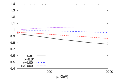
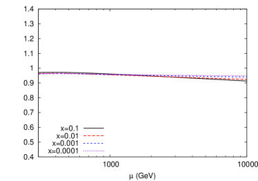
We see that for the top-quark PDF at NLO, the difference between the 2-loop approximated PDF $\tilde{t}^{(2)}(x,\mu^{2})$ and the fully evolved PDF $t(x,\mu^{2})$ is very small (of the order of $5$%) unless very high scales and large $x$ are involved. A comparable behaviour was observed in Ref. Dawson:2014pea .

3 Different heavy quark schemes: numerical results

In this Section, we consider the production of Higgs and neutral vector bosons via $b\bar{b}$ fusion at the LHC and the production of heavy vector bosons in $t\bar{t}$ collisions at a future high energy hadron collider. We compare predictions for total rates obtained at the highest available perturbative order in the 4F and 5F schemes at the LHC and in the 5F and 6F schemes at a future 100 TeV collider.

3.1 LHC Run II

3.1.1 Bottom-fusion initiated Higgs production

Although in the SM the fully-inclusive $b\bar{b}\to H$ cross section is much smaller than the other Higgs production channels (gluon fusion, vector boson fusion, $W$ and $Z$ associated Higgs production) and its rate further decreases when acceptance cuts on the associated $b$ quarks are imposed, this production process can be important in several non-standard scenarios. For example, in supersymmetric models Higgs production in association with $b$ quarks can become a dominant production channel when couplings are enhanced with respect to the Standard Model. More specifically, in models featuring a second Higgs doublet the rate is typically increased by a factor $1/\cos^{2}\beta$ or $\tan^{2}\beta$, with $\beta=v_{1}/v_{2}$ being the ratio of two Higgs vacuum expectation values.

Calculations for $b$-initiated Higgs productions have been made available by several groups. The total cross section for this process is currently known up to next-to-next-to-leading order (NNLO) in the 5F scheme Harlander:2003ai and up to next-to-leading order (NLO) in the 4F scheme Dittmaier:2003ej ; Dawson:2005vi . Total cross section predictions have been also obtained via matching procedures that include the resummation of the collinear logarithms on one side and the mass effects on the other, without double counting common terms. A first heuristic proposal, which has been adopted for some time by the HXSWG LHC, is based on the so-called Santander matching Harlander:2011aa where an interpolation between results in the 4F and in the 5F schemes is obtained by means of a weighted average of the two results. Several groups have provided properly matched calculations based on a thorough quantum field theory analysis, at NLO+NLL and beyond via the FONLL method Forte:2015hba and an effective field theory approach Bonvini:2015pxa ; Bonvini:2016fgf that yield very similar results.

Fully differential calculations in the 4F scheme up to NLO(+PS) accuracy have been recently made available Wiesemann:2014ioa in MadGraph5_aMC@NLO  Alwall:2014hca and work is in progress in the SHERPA  framework Gleisberg:2008ta . These studies conclude that the 4F scheme results, thanks to the matching to parton showers, are generally more accurate than the pure 5F scheme counterparts, especially for observables which are exclusive in the $b$-quark kinematics. On the other hand, for inclusive observables the differences between 4F and 5F schemes are mild if judicious choices for scales are made. The assessment of the size of such effects and their relevance for phenomenology is the purpose of this section.

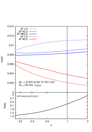
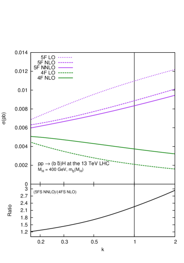
We first compare the size and the scale dependence of the 4F and 5F scheme predictions from leading-order up to the highest available perturbative order, namely NLO in the case of the 4F scheme and NNLO in the case of the 5F scheme cross sections. Results are shown in Figs. 5 and 6 for the SM Higgs ($M_{H}=125$ GeV) and a heavier Higgs ($M_{H}=400$ GeV) respectively. The 4F scheme cross section has been generated using the public version of MadGraph5_aMC@NLO Alwall:2014hca . In the case of the 5F scheme calculation, the cross section has been computed with SusHi Harlander20131605 and the LO and NLO results have been cross-checked against the output of MadGraph5_aMC@NLO. The input PDFs belong to the NNPDF3.0 family Ball:2014uwa and the $n_{f}=4$ set was used in association with the 4F scheme calculation, while the $n_{f}=5$ set was associated with the 5F scheme calculation, consistently with the perturbative order of the calculation, and with $\alpha_{s}^{\rm 5F}(M_{Z})=0.118$. Both the renormalisation and factorisation scales have been taken to be equal to $kM_{H}$, with $0.15\leq k\leq 2$.

The treatment of the Higgs Yukawa coupling to $b$ quarks deserves some attention. Different settings may cause large shifts in theoretical predictions. Here we use the $\overline{\mbox{\small MS}}$ scheme; the running $b$ Yukawa $y_{b}(\mu)$ is computed at the scale $\mu_{R}$ (left plots). We have checked that computing the Yukawa at the fixed value of $M_{H}$ does not modify our conclusions (right plots). The numerical value of $m_{b}(\mu_{R})$ is obtained from $m_{b}(m_{b})$ by evolving up to $\mu_{R}$ at 1-loop (LO), 2-loops (NLO) or 3-loops (NNLO) with $n_{f}=4$ or $n_{f}=5$, depending on the scheme. The numerical value of $m_{b}(m_{b})$ is taken to be equal to the pole mass $m_{b}^{\rm pole}=4.75$ GeV at LO (in both the 4F and 5F schemes), $m_{b}(m_{b})=4.16$ GeV at NLO in the 5F scheme and $m_{b}(m_{b})=4.34$ GeV in the 4F scheme (consistently with the settings adopted in Ref. Wiesemann:2014ioa ) and finally $m_{b}(m_{b})=4.18$  GeV at NNLO in the 5F scheme, consistently with the latest recommendation of the Higgs cross section working group.

Figure 5: Cross sections for the production of the SM Higgs boson via $b\bar{b}$ fusion ($y_{b}^{2}$ term only) in the 5F and 4F schemes for LHC 13 TeV as functions of $k=\mu/M_{H}$, with $\mu_{F}=\mu_{R}=\mu$. Terms proportional to $y_{b}y_{t}$ in the NLO 4F scheme have been neglected. Results with the running $b$ mass computed at a fixed scale $M_{H}$ are also shown (right plot). In the inset the ratio between the 5F NNLO prediction and the 4F scheme NLO prediction is displayed.

Figure 6: Same as Fig. 5 with $M_{H}=$ 400 GeV

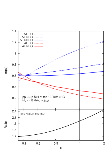
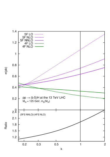
The 4F and 5F scheme curves at leading order show an opposite behaviour: in the 4F scheme the scale dependence is driven by the running of $\alpha_{s}$ and therefore decreases with the scale, while the 5F scheme case it is determined by the scale dependence of the $b$-quark PDF which in turn leads to an increase. The inclusion of higher orders in both calculations drastically reduces the differences; nonetheless, it is clear from Figs. 5 and 6 that around the central scale $k=1$ the best 5F scheme prediction exceeds the highest order 4F scheme prediction by a large amount, about 80%. We also observe that 4F and 5F scheme predictions are closer at lower values of the scale. The scale dependence of the 4F scheme NLO calculation is approximately of the same size as that of the 5F scheme NLO calculation, while it is stronger than the scale dependence of the 5F scheme NNLO calculation, as expected, since in the latter the collinear logarithms are resummed.

In Fig. 6 the same curves are displayed for a heavier Higgs, $M_{H}=400$ GeV. As observed in Ref. Maltoni:2012pa , for heavier final state particles differences between schemes are enhanced. In particular, at the central scale the NNLO 5F scheme prediction exceeds the 4F scheme case by a factor of two. Also in this case, at smaller values of the scale the difference is significantly reduced.

This behaviour corresponds to that expected from our analysis presented in sect. 2. Comparing calculations at ${\tilde{\mu}}_{F}=0.36\,M_{H}$ for $M_{H}=125$ GeV and ${\tilde{\mu}}_{F}=0.29\,M_{H}$ for $M_{H}=400$ GeV, the differences between the predictions in the 4F and 5F scheme reduce to about 30-35%, a difference that can be accounted for by considering first the (positive) effects of resummation included in the 5F scheme calculation with respect to the 4F one and second the power-like quark-mass corrections that are not included the 5F calculation and estimated to be around $-$2-5%, see Ref. Forte:2015hba ; Bonvini:2015pxa ; Bonvini:2016fgf .

The effects of the resummation are easy to quantify by establishing the range of $x$ which gives the dominant contribution to Higgs production via $b\bar{b}$ collisions. To this purpose, we show in Fig. 7 the $x$ distribution in the leading-order bottom-quark fusion Higgs production in the 5F scheme.

Figure 7: Normalised distribution of the momentum fraction $x$ carried by the $b$ quark in $b\bar{b}$ initiated Higgs production, in the 5F scheme at leading order for LHC 13 TeV, for $M_{H}=125$ GeV (red curve) and $M_{H}=400$ GeV (blue curve).

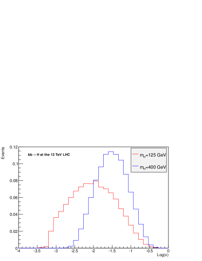
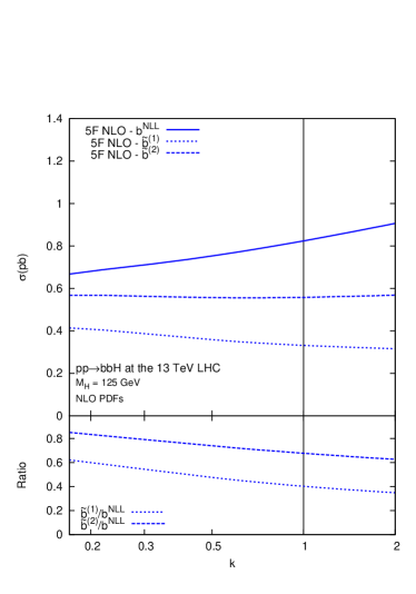
We observe that the $x$ distribution has its maximum around $x\approx 10^{-2}$ for the Standard Model Higgs; for such values of $x$, the resummation of collinear logarithms is sizeable: the difference between the fully resummed $b$ PDF and $\tilde{b}^{(2)}$ becomes as large as 10 to 15% for scales between 100 and 400 GeV. Note that we expect twice the effect of a single $b$ quark in the case of processes with two $b$ quarks in the initial state, which amounts to a difference of 20-25% from resummed logarithms at ${\cal O}(\alpha_{s}^{3})$ and higher between the collinear approximation of the 4F scheme calculation and the 5F scheme calculation.

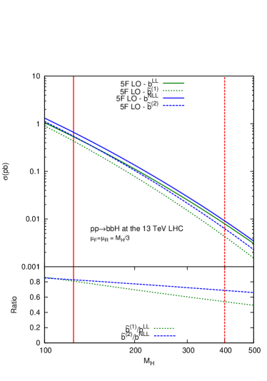
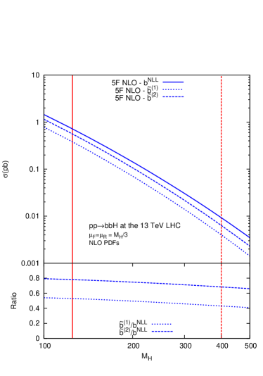
This expectation is confirmed by the curves in Fig. 8, where we plot the 5F scheme cross section at LO (left panel) and NLO (right panel) as a function of the Higgs mass in the range 100 GeV to 500 GeV, with $\mu_{R}=\mu_{F}=M_{H}/3$. The cross sections are computed with the same settings as in Fig. 5. In the same panel we present the cross sections with the $b$ PDF replaced by the $\tilde{b}^{(p)}$ truncated PDF computed at order $p=1$ and at order $p=2$, together with the relevant ratios. We observe that, for a sensible value of the factorisation and renormalisation scales, as per the one suggested in this paper $\tilde{\mu}_{F}\sim M_{H}/3$, the effect of neglecting the higher order logs resummed in the $b$ PDF evolution beyond the ones included in the second order expansion of the $b$ PDF, $\tilde{b}^{(2)}$, is smaller than 20% for the SM Higgs mass and of about 30% for a heavier Higgs. Similar conclusions are drawn if the NLO cross section is considered instead, as in the right hand-side panel. If instead we had taken as the central scale choice $\mu_{R}=\mu_{F}=M_{H}$ the effects of the resummation of higher order logs would appear much more significant.

Figure 8: Higgs production cross section via $b\bar{b}$ fusion at LO (left) and NLO (right) as a function of $M_{H}$, computed either with the fully resummed $b$ quark PDF at LL or NLL, or with the truncated PDF $\tilde{b}^{(p)}$ with $p=1,2$, with $\mu=\mu_{F}=\mu_{R}=M_{H}/3$.

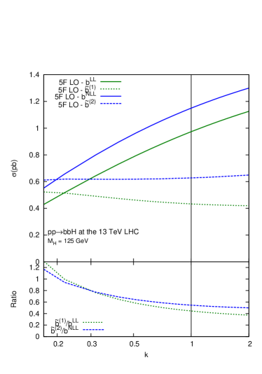
The scale dependence of the Standard Model Higgs cross section is studied in Fig. 9. The plots confirm the findings that the assessment of the effect of the higher-order logs resummed in a 5F scheme calculation strongly depends on the scale at which the process is computed and that at a scale close to $\tilde{\mu}_{F}$ the effects of higher order logs are quite moderate, while they become significant if the naive hard scle of the process is chosen.

Figure 9: Standard Model Higgs production cross section via $b\bar{b}$ fusion at LO (left) and NLO (right) as a function of $k=\mu/M_{H}$, with $\mu=\mu_{R}=\mu_{F}$, computed either with the fully resummed $b$ quark PDF at LL or NLL, or with the truncated PDF $\tilde{b}^{(p)}$ with $p=1,2$.

3.1.2 Bottom-fusion initiated $Z^{\prime}$ production

A similar analysis can be carried out for the case of $Z$ production. $Z$-boson production in association with one or two $b$-jets has a very rich phenomenology. It is interesting as a testbed of our understanding of QCD and it enters in precision measurements (Drell-Yan at the LHC or indirectly in the $W$ mass determination). In addition, it represents a crucial irreducible background for several Higgs production channels at the LHC. For the SM Higgs boson, $Zb\bar{b}$ production is a background to $ZH$ associated production followed by the decay of the Higgs into a bottom-quark pair. Finally, this process is a background to searches for Higgs bosons with enhanced $Hb\bar{b}$ Yukawa coupling.

Calculations for bottom-initiated $Z$ production have been made available by several groups. The $Zb\bar{b}$ production cross section was originally computed (neglecting the $b$ quark mass) in Ref. Campbell:2000bg for exclusive 2-jet final states. The effect of a non-zero $b$ quark mass was considered in later works FebresCordero:2008ci ; Cordero:2009kv where the total cross section was also given. More recently, in Ref. Frederix:2011qg leptonic decays of the $Z$ boson have taken into account, together with the full correlation of the final state leptons and the parton shower and hadronisation effects. The total cross section for $Zb\bar{b}$ in the 5F scheme has been computed at NNLO accuracy for the first time in Ref. Maltoni:2005wd .

Bottom-initiated $Z$ production is in principle very different from Higgs production because the $Z$ boson has a non-negligible coupling to the light quarks. For simplicity, we will not take these couplings into account; to avoid confusion, we refer to the $Z$ boson that couples only with heavy quarks as $Z^{\prime}$, even when we take its mass to be equal to $91.2$ GeV as in the Standard Model.

We have calculated the 5F scheme cross sections by using a private code Maltoni:2005wd , which has been cross-checked at LO and NLO against MadGraph5_aMC@NLO. The 4F scheme cross section has been computed with MadGraph5_aMC@NLO. Our settings are the same as in the Higgs production computation. We take the same value $\mu$ for the factorisation and renormalisation scales.

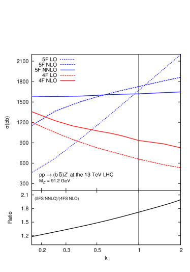
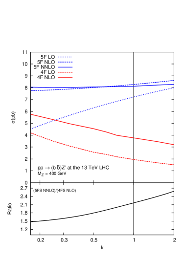
Results are presented in Fig. 10 as functions of $k=\mu/M_{Z^{\prime}}$ for $M_{Z^{\prime}}=91.2$ GeV and $M_{Z^{\prime}}=400$ GeV respectively. We observe that for $\mu=M_{Z^{\prime}}$ the best 5F scheme prediction exceeds the 4F scheme prediction by almost 30%, while their difference is reduced at lower values of the scales. In this respect the behaviour of the 4F vs 5F scheme predictions reflects what we have already observed in Fig. 5. We note, however, that the scale dependence of the 5F scheme predictions for $Zb\bar{b}$ is quite different with respect to the $Hb\bar{b}$ when $m_{H}=125$ GeV. In the case of $Zb\bar{b}$ is quite mild already at NLO and the perturbative expansion seems to converge more quickly for higher values of $\mu$ around $\mu=M_{Z^{\prime}}$. The behaviour of the 5F calculations for $M_{H}=M_{Z^{\prime}}=400$ GeV cases, on the other hand, do not show any significant qualitative difference, apart from the fact that $Zb\bar{b}$ results have in general a milder scale dependence. The different scale sensitivity (with $\mu_{R}=\mu_{F}$) of the two processes can be traced back to the fact that while the Yukawa interaction renormalises under QCD, the EW current (and corresponding charge) is conserved, resulting in general in a milder scale dependence of the $Zb\bar{b}$ predictions.

Figure 10: Cross sections for bottom-fusion initiated $Z^{\prime}$ boson production in the 5F and 4F schemes for LHC 13 TeV as functions of $k=\mu/M_{Z^{\prime}}$. $M_{Z^{\prime}}=91.2$ GeV (left) and $M_{Z^{\prime}}=400$ GeV (right). Settings are specified in the text.

3.2 Future Colliders

The perspective of a proton-proton collider at a centre–of–mass energy of 100 TeV would open up a new territory beyond the reach of the LHC. New heavy particles associated with new physics sector may be discovered and new interactions unveiled. At such large energies, essentially all SM particles can be considered as massless, including the top quarks. We therefore expect collinear enhancements in top-quark initiated processes. In Ref. Dawson:2014pea the question of whether the top quark should be treated as an ordinary parton at high centre-of-mass energy, thereby defining a 6FNS, is scrutinised, and the impact of resumming collinear logs of the top quark mass is assessed. This analysis is performed in the context of charged Higgs boson production at 100 TeV. In Ref. Han:2014nja , the impact of resumming initial-state collinear logarithms in the associated heavy Higgs ($M_{H}>5$ TeV) and top pair production (with un-tagged top quarks) is examined and it is found to be very large at large Higgs masses.

In Fig. 11 the total cross sections for the production of a $Z^{\prime}$ boson of mass $M_{Z^{\prime}}=$ 1 TeV (left), $M_{Z^{\prime}}=$ 5 TeV (centre), $M_{Z^{\prime}}=$ 10 TeV (right) are plotted in the 5F and 6F schemes as a function of the renormalisation and factorisation scales, which are identified and varied between $0.2M_{Z^{\prime}}$ and $2M_{Z^{\prime}}$. Results are obtained by using MadGraph5_aMC@NLO for the 5F scheme and a private code for the 6F scheme. Results in the 6F scheme have been cross- checked up to NLO against MadGraph5_aMC@NLO. We have set $m_{t}^{\rm pole}=172.5$ GeV and turned off the coupling of the $Z^{\prime}$ heavy boson to all lighter quarks.

Figure 11: Cross sections for $t\bar{t}$ initiated $Z^{\prime}$ production in the 6F and 5F schemes at a 100 TeV $pp$ collider as functions of $k=\mu/M_{Z^{\prime}}$. Top mass: $m_{t}=173$ GeV. Mass of the heavy boson: $M_{Z^{\prime}}=$ 1 TeV (left), $M_{Z^{\prime}}=$ 5 TeV (centre), $M_{Z^{\prime}}=$ 10 TeV (right). The inlay below shows the ratio of the cross sections in the 6F and 5F schemes.

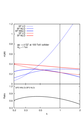
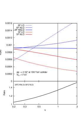
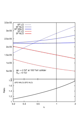
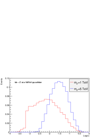
Firstly, we observe that the $M_{Z^{\prime}}=$ 1 TeV case is quite different from the $M_{Z^{\prime}}=$ 5 TeV and $M_{Z^{\prime}}=$ 10 TeV, which in turn display a very similar pattern to the $b$ initiated processes with similar $m_{Q}/M_{Z^{\prime}}$ and $M_{Z^{\prime}}/\sqrt{s}$ ratios. The behaviour of the leading-order cross section in the 6F scheme for $M_{Z^{\prime}}=$ 1 TeV is mitigated at higher masses and at higher orders (NLO). At NNLO the 6F-scheme cross section displays a similar scale dependence as the NLO cross section in the 5F scheme with a residual difference of about 40% between the two best predictions in the two schemes. To further investigate these differences, in Fig. 12 we plot the distribution of the fraction of momentum carried by the top quarks for $M_{Z^{\prime}}=$ 1 TeV and $M_{Z^{\prime}}=$ 5 TeV in the 6F schemes. As expected, compared to heavier masses, the production of a $M_{Z^{\prime}}=$ 1 TeV happens mostly at threshold and it is dominated by smaller values of Bjorken $x$. The ratio $M_{Z^{\prime}}/m_{t}\simeq 6$ is not very large to start with (for comparison $M_{Z}/m_{b}\simeq 20$) and initial-state quark collinear configurations are not dominant. We conclude that in the $M_{Z^{\prime}}=$ 1 TeV case the differences between the two schemes are to be associated to the absence of power-like mass terms in the 6F calculation.

Figure 12: Normalised distribution of momentum fraction $x$ carried by the $t\bar{t}$ initiated $Z^{\prime}$ production in the 6F scheme distributions at LO in a 5F scheme for $M_{Z^{\prime}}=1$ TeV and $M_{Z^{\prime}}=5$ TeV at a 100 TeV collider. Events were generated at values of the scales $\mu_{R}=\mu_{F}=H_{T}/4$. Input PDF: NNPDF30 LO $n_{f}=5$ ($\alpha_{s}(M_{Z})=0.130$).

4 Conclusions

In this work we have considered the use of four- and five-flavour schemes in precision physics at the LHC and in the context of $b$-initiated Higgs and $Z$ production. We have extended previous work done for processes involving a single $b$ quark in the initial state to cases in which two are present. We have followed a “deconstructing” methodology where the impacts of the various sources of differences between the schemes have been evaluated one by one.

Firstly, we have obtained the form of the collinear logarithms in the four-flavour scheme by performing the explicit computation of the $2\to 3$ body scattering process and studying the collinear limit using as natural variables the $t$-channel invariants. We have then compared the resulting expression with the corresponding cross section in the 5-flavor scheme as calculated by only keeping the explicit log in the $b$-quark PDF, i.e. without resummation. This has allowed us to assess the analytic form and therefore the size of the collinear logarithms and to propose a simple procedure to identify the relevant scales in the processes where the results in the two schemes should be evaluated and compared. In so doing we have considered cases where power-like effects in the mass of the heavy quarks were assumed (and then checked a posteriori by comparing to the full result) unimportant. Secondly, we have explicitly estimated the effects of the resummation by studying fully evolved $b$ PDF with truncated expansions at finite order.

We have then applied our general approach to the case of Higgs and $Z$ boson production in association with $b$ quarks at the LHC and to heavy $Z^{\prime}$ production in association with top quarks at a future 100 TeV collider. We have found that the resummation increases the cross section in most cases by about 20% (sometimes reaching 30%) at the LHC and in general leads to a better precision. On the other hand, the 4F scheme predictions (5F scheme in the case of associated top-quark production) at NLO also display a consistent perturbative behaviour when evaluated at suitable scales. They should therefore should be used when the heavy-quark mass effects are not negligible and to predict distributions involving the heavy quarks in the final state.

Appendix A Cross section in the collinear limit

In this Appendix we illustrate in some detail the calculation of the cross section for the partonic process

$$g(p_{1})+g(p_{2})\to b(k_{1})+\bar{b}(k_{2})+H(k)$$ (28)

in the limit of collinear emission of $b$ quarks. We choose, as independent kinematic invariants,

$$\hat{s} = (p_{1}+p_{2})^{2}=2p_{1}p_{2}$$ (29)

$$t_{1} = (p_{1}-k_{1})^{2}=-2p_{1}k_{1}+m_{b}^{2}$$ (30)

$$t_{2} = (p_{2}-k_{2})^{2}=-2p_{2}k_{2}+m_{b}^{2}$$ (31)

$$s_{1} = (k_{1}+k)^{2}=2k_{1}k+m_{b}^{2}+M_{H}^{2}$$ (32)

$$s_{2} = (k_{2}+k)^{2}=2k_{2}k+m_{b}^{2}+M_{H}^{2}.$$ (33)

The remaining invariants

$$u_{1} =(p_{1}-k_{2})^{2}=-2p_{1}k_{2}+m_{b}^{2}$$ (34)

$$u_{2} =(p_{2}-k_{1})^{2}=-2p_{2}k_{1}+m_{b}^{2}$$ (35)

$$s_{12} =(k_{1}+k_{2})^{2}=2k_{1}k_{2}+2m_{b}^{2}$$ (36)

$$t =(p_{1}-k)^{2}-M_{H}^{2}=-2kp_{1}$$ (37)

$$u =(p_{2}-k)^{2}-M_{H}^{2}=-2kp_{2}$$ (38)

are related to the independent invariants by

$$u_{1}=s_{1}-\hat{s}-t_{2}+m_{b}^{2}$$ (39)

$$u_{2}=s_{2}-\hat{s}-t_{1}+m_{b}^{2}$$ (40)

$$t=-s_{1}+t_{2}-t_{1}+m_{b}^{2}$$ (41)

$$u=-s_{2}+t_{1}-t_{2}+m_{b}^{2}$$ (42)

$$s_{12}=\hat{s}-s_{1}-s_{2}+M_{H}^{2}+2m_{b}^{2}.$$ (43)

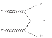
The leading-order Feynman diagrams are shown in Fig. 13.

Figure 13: Leading order diagrams for $gg\to b\bar{b}H$.

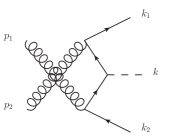
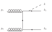
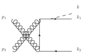
The squared invariant amplitude (averaged over initial state summed over final state spin and color variables) has the general structure

$$\left|\mathcal{M}\right|^{2}=\frac{G(s,s_{1},s_{2},t_{1},t_{2})}{(t_{1}-m_{b}^{2})^{2}(t_{2}-m_{b}^{2})^{2}(u_{1}-m_{b}^{2})^{2}(u_{2}-m_{b}^{2})^{2}}.$$ (44)

The function $G(s,s_{1},s_{2},t_{1},t_{2})$ is a polynomial in $t_{1},t_{2}$. It can be shown on general grounds Keller:1998tf ; Catani:2000ef that each double pole is suppressed by a factor of $m_{b}^{2}$. Furthermore, it is well known that collinear singularities do not arise in interference terms among different amplitudes. Thus,

$$\left|\mathcal{M}\right|^{2}=\frac{G_{t}}{(t_{1}-m_{b}^{2})(t_{2}-m_{b}^{2})}+\frac{G_{u}}{(u_{1}-m_{b}^{2})(u_{2}-m_{b}^{2})}+\left|\mathcal{M}\right|^{2}_{\rm reg}$$ (45)

where the term $\left|\mathcal{M}\right|^{2}_{\rm reg}$ does not give rise to collinear singularities in the limit $m_{b}=0$. An explicit calculation gives

$$G_{t}=G_{u}=\frac{32\alpha_{s}^{2}\pi^{2}m_{b}^{2}G_{F}M_{H}^{2}\sqrt{2}}{3}\frac{P_{qg}(z_{1})}{z_{1}}\frac{P_{qg}(z_{2})}{z_{2}},$$ (46)

where

$$z_{1}=\frac{M_{H}^{2}}{s_{1}};\qquad z_{2}=\frac{M_{H}^{2}}{s_{2}}$$ (47)

and $P_{qg}(z)$ is defined in Eq. (11).

The 3-body phase-space invariant measure

$$d\phi_{3}(p_{1},p_{2};k_{1},k_{2},k)$$

$$=\frac{d^{3}k_{1}}{(2\pi)^{3}2k_{1}^{0}}\frac{d^{3}k_{2}}{(2\pi)^{3}2k_{2}^{0}}\frac{d^{3}k}{(2\pi)^{3}2k^{0}}(2\pi)^{4}\delta(p_{1}+p_{2}-k_{1}-k_{2}-k)$$ (48)

can be factorised as

$$d\phi_{3}(p_{1},p_{2};k_{1},k_{2},k)=\frac{dt_{1}}{2\pi}\frac{dt_{2}}{2\pi}d\phi_{2}(p_{1};k_{1},q_{1})d\phi_{2}(p_{2};k_{2},q_{2})d\phi_{1}(q_{1},q_{2};k),$$ (49)

where

$$q_{1}^{2}=t_{1};\qquad q_{2}^{2}=t_{2}.$$ (50)

We now compute each factor explicitly. We have

$$d\phi_{2}(p_{1};k_{1},q_{1}) =\frac{d^{3}k_{1}}{(2\pi)^{3}2k_{1}^{0}}\frac{d^{3}q_{1}}{(2\pi)^{3}2q_{1}^{0}}(2\pi)^{4}\delta(p_{1}-k_{1}-q_{1})$$

$$=\frac{1}{16\pi^{2}}\frac{|\vec{k}_{1}|^{2}d|\vec{k}_{1}|d\cos\theta_{1}d\phi_{1}}{k_{1}^{0}q_{1}^{0}}\delta(p_{1}^{0}-k_{1}^{0}-q_{1}^{0})$$ (51)

where

$$k_{1}^{0}=\sqrt{|\vec{k}_{1}|^{2}+m_{b}^{2}}$$ (52)

$$q_{1}^{0}=\sqrt{{|\vec{p}_{1}|}^{2}+|\vec{k}_{1}|^{2}-2|\vec{p}_{1}||\vec{k}_{1}|\cos\theta_{1}+t_{1}}$$ (53)

We may now integrate over $\cos\theta_{1}$ using the delta function

$$\delta(p_{1}^{0}-k_{1}^{0}-q_{1}^{0})=\frac{q_{1}^{0}}{|\vec{p}_{1}||\vec{k}_{1}|}\delta(\cos\theta_{1}-\cos\bar{\theta}_{1})$$ (54)

with $\bar{\theta}_{1}$ a solution of

$$p_{1}^{0}-\sqrt{|\vec{k}_{1}|^{2}+m_{b}^{2}}-\sqrt{|\vec{p}_{1}|^{2}+|\vec{k}_{1}|^{2}-2|\vec{p}_{1}||\vec{k}_{1}|\cos\bar{\theta}_{1}+t_{1}}=0.$$ (55)

This gives

$$d\phi_{2}(p_{1};k_{1},q_{1})=\frac{1}{16\pi^{2}}\frac{|\vec{k}_{1}|d|\vec{k}_{1}|d\varphi_{1}}{k_{1}^{0}|\vec{p}_{1}|};\qquad d\phi_{2}(p_{2};k_{2},q_{2})=\frac{1}{16\pi^{2}}\frac{|\vec{k}_{2}|d|\vec{k}_{2}|d\varphi_{2}}{k_{2}^{0}|\vec{p}_{2}|}$$ (56)

and therefore

$$d\phi_{3}(p_{1},p_{2};k_{1},k_{2},k)=\frac{1}{1024\pi^{6}}dt_{1}dt_{2}\frac{|\vec{k}_{1}|d|\vec{k}_{1}|d\varphi_{1}}{k_{1}^{0}|\vec{p}_{1}|}\frac{|\vec{k}_{2}|d|\vec{k}_{2}|d\varphi_{2}}{k_{2}^{0}|\vec{p}_{2}|}d\phi_{1}(q_{1},q_{2};k).$$ (57)

It will be convenient to adopt the centre-of-mass frame, where

$$p_{1}=\frac{\sqrt{\hat{s}}}{2}(1,0,0,1),\qquad p_{2}=\frac{\sqrt{\hat{s}}}{2}(1,0,0,-1)$$ (58)

In this frame

$$s_{1}=(k+k_{1})^{2}=(p_{1}+p_{2}-k_{2})^{2}=\hat{s}+m_{b}^{2}-2\sqrt{\hat{s}}\sqrt{|\vec{k}_{2}|^{2}+m_{b}^{2}}$$ (59)

$$s_{2}=(k+k_{2})^{2}=(p_{1}+p_{2}-k_{1})^{2}=\hat{s}+m_{b}^{2}-2\sqrt{\hat{s}}\sqrt{|\vec{k}_{1}|^{2}+m_{b}^{2}}$$ (60)

and therefore

$$\frac{|\vec{k}_{1}|d|\vec{k}_{1}|}{k_{1}^{0}|\vec{p}_{1}|}\frac{|\vec{k}_{2}|d|\vec{k}_{2}|}{k_{2}^{0}|\vec{p}_{2}|}=\frac{ds_{1}}{\hat{s}}\frac{ds_{2}}{\hat{s}}.$$ (61)

Furthermore, we may use the invariance of the cross section upon rotations about the $z$ axis to replace

$$d\varphi_{1}d\varphi_{2}\to 2\pi d\varphi;\qquad\varphi=\varphi_{1}-\varphi_{2}.$$ (62)

Finally,

$$d\phi_{1}(q_{1},q_{2};k)=2\pi\delta\left((q_{1}+q_{2})^{2}-M_{H}^{2}\right),$$ (63)

and therefore

$$d\phi_{3}(p_{1},p_{2};k_{1},k_{2},k)=\frac{1}{256\pi^{4}\hat{s}^{2}}ds_{1}ds_{2}dt_{1}dt_{2}\,d\varphi\delta\left((q_{1}+q_{2})^{2}-M_{H}^{2}\right).$$ (64)

It is a tedious, but straightforward, task to show that, upon integration over the azimuth $\varphi$ using the delta function, this expression is the same as the one given in Byckling:1971vca for the three-body phase-space measure in terms of four invariants.

The two invariants $u_{1},u_{2}$ are related to independent invariants through Eqs. (39,40), which can be written

$$u_{1}-m_{b}^{2}=-(t_{2}-a_{2})$$ (65)

$$u_{2}-m_{b}^{2}=-(t_{1}-a_{1})$$ (66)

where we have defined

$$a_{1}=s_{2}-\hat{s};\qquad a_{2}=s_{1}-\hat{s}.$$ (67)

The bounds for $t_{1}$ are easily obtained. In the centre-of-mass frame we have

$$t_{1}= \frac{1}{2}\left[a_{1}+m_{b}^{2}-\cos\bar{\theta}_{1}\sqrt{(a_{1}+m_{b}^{2})^{2}-4m_{b}^{2}(a_{1}+\hat{s})}\right]$$ (68)

$$t_{2}= \frac{1}{2}\left[a_{2}+m_{b}^{2}+\cos\bar{\theta}_{2}\sqrt{(a_{2}+m_{b}^{2})^{2}-4m_{b}^{2}(a_{2}+\hat{s})}\right].$$ (69)

The upper and lower bound are obtained for $\cos\bar{\theta}_{1}=\pm 1$, $\cos\bar{\theta}_{2}=\pm 1$. We get

$$t_{1}^{-}\leq t_{1}\leq t_{1}^{+};\qquad t_{2}^{-}\leq t_{2}\leq t_{2}^{+},$$ (70)

where

$$t_{1}^{\pm}=\frac{1}{2}\left[a_{1}+m_{b}^{2}\pm\sqrt{(a_{1}+m_{b}^{2})^{2}-4m_{b}^{2}(a_{1}+\hat{s})}\right]$$ (71)

$$t_{2}^{\pm}=\frac{1}{2}\left[a_{2}+m_{b}^{2}\pm\sqrt{(a_{2}+m_{b}^{2})^{2}-4m_{b}^{2}(a_{2}+\hat{s})}\right].$$ (72)

For small $m_{b}^{2}$,

$$t_{i}^{+}=m_{b}^{2}+\frac{m_{b}^{2}\hat{s}}{a_{i}}+O(m^{4});\qquad t_{i}^{-}=a_{i}-\frac{m_{b}^{2}\hat{s}}{a_{i}}+O(m^{4});\qquad i=1,2.$$ (73)

All the ingredients to compute the total partonic cross section in the collinear limit are now available. In this limit, the relative azimuth $\phi$ between $b$ and $\bar{b}$ is irrelevant, and simply provides a factor of $2\pi$. Furthermore

$$\hat{s}=\frac{M_{H}^{2}}{z_{1}z_{2}};\qquad s_{1}=\hat{s}z_{2};\qquad s_{2}=\hat{s}z_{1}$$ (74)

and therefore

$$\frac{ds_{1}\,ds_{2}}{\hat{s}^{2}}=dz_{1}\,dz_{2}.$$ (75)

The integrals over $t_{1},t_{2}$ are easily computed:

$$\int_{t_{i}^{-}}^{t_{i}^{+}}dt_{i}\,\frac{1}{t_{i}-m_{b}^{2}}=\log\frac{a_{1}^{2}}{m_{b}^{2}\hat{s}}+O(1)=\log\frac{M_{H}^{2}}{m_{b}^{2}}\frac{(1-z_{i})^{2}}{z_{1}z_{2}}$$ (76)

$$\int_{t_{i}^{-}}^{t_{i}^{+}}dt_{i}\,\frac{1}{t_{i}-a_{i}}=-\log\frac{a_{i}^{2}}{m_{b}^{2}\hat{s}}+O(1)=-\log\frac{M_{H}^{2}}{m_{b}^{2}}\frac{(1-z_{i})^{2}}{z_{1}z_{2}}+O(1).$$ (77)

Finally,

$$\delta\left((q_{1}+q_{2})^{2}-M_{H}^{2}\right)=\delta(z_{1}z_{2}\hat{s}-M_{H}^{2}).$$ (78)

We find

$$\hat{\sigma}^{\rm 4F,coll}(\hat{\tau}) =\frac{1}{2\hat{s}}\int d\phi_{3}(p_{1},p_{2};k_{1},k_{2},k)\,G_{u}\left[\frac{1}{(t_{1}-m_{b}^{2})(t_{2}-m_{b}^{2})}+\frac{1}{(t_{1}-a_{1})(t_{2}-a_{2})}\right]$$

$$=\hat{\tau}\frac{\alpha_{s}^{2}}{4\pi^{2}}\frac{m_{b}^{2}}{M_{H}^{2}}\frac{G_{F}\pi}{3\sqrt{2}}2\int_{0}^{1}dz_{1}\int_{0}^{1}dz_{2}\,\delta(z_{1}z_{2}-\hat{\tau})$$

$$\times P_{qg}(z_{1})\log\left[\frac{M_{H}^{2}}{m_{b}^{2}}\frac{(1-z_{1})^{2}}{\hat{\tau}}\right]P_{qg}(z_{2})\log\left[\frac{M_{H}^{2}}{m_{b}^{2}}\frac{(1-z_{2})^{2}}{\hat{\tau}}\right].$$ (79)

References

- (1) F. Maltoni, G. Ridolfi, and M. Ubiali, b-initiated processes at the LHC: a reappraisal, JHEP 1207 (2012) 022, [arXiv:1203.6393].
- (2) S. Dawson, C. B. Jackson, L. Reina, and D. Wackeroth, Exclusive Higgs boson production with bottom quarks at hadron colliders, Phys. Rev. D69 (2004) 074027, [hep-ph/0311067].
- (3) F. Maltoni, Z. Sullivan, and S. Willenbrock, Higgs-boson production via bottom-quark fusion, Phys. Rev. D67 (2003) 093005, [hep-ph/0301033].
- (4) J. M. Campbell, S. Dawson, S. Dittmaier, C. Jackson, M. Kramer, et al., Higgs boson production in association with bottom quarks, hep-ph/0405302.
- (5) R. Harlander, M. Kramer, and M. Schumacher, Bottom-quark associated Higgs-boson production: reconciling the four- and five-flavour scheme approach, arXiv:1112.3478.
- (6) M. Wiesemann, R. Frederix, S. Frixione, V. Hirschi, F. Maltoni, and P. Torrielli, Higgs production in association with bottom quarks, JHEP 02 (2015) 132, [arXiv:1409.5301].
- (7) J. M. Campbell and R. K. Ellis, Radiative corrections to Z b anti-b production, Phys. Rev. D62 (2000) 114012, [hep-ph/0006304].
- (8) F. Febres Cordero, L. Reina, and D. Wackeroth, NLO QCD corrections to production with massive bottom quarks at the Fermilab Tevatron, Phys. Rev. D78 (2008) 074014, [arXiv:0806.0808].
- (9) F. Febres Cordero, L. Reina, and D. Wackeroth, W- and Z-boson production with a massive bottom-quark pair at the Large Hadron Collider, Phys. Rev. D80 (2009) 034015, [arXiv:0906.1923].
- (10) R. Frederix, S. Frixione, V. Hirschi, F. Maltoni, R. Pittau, and P. Torrielli, W and boson production in association with a bottom-antibottom pair, JHEP 09 (2011) 061, [arXiv:1106.6019].
- (11) M. Bonvini, A. S. Papanastasiou, and F. J. Tackmann, Resummation and matching of b-quark mass effects in production, JHEP 11 (2015) 196, [arXiv:1508.03288].
- (12) S. Forte, D. Napoletano, and M. Ubiali, Higgs production in bottom-quark fusion in a matched scheme, Phys. Lett. B751 (2015) 331–337, [arXiv:1508.01529].
- (13) M. Bonvini, A. S. Papanastasiou, and F. J. Tackmann, Matched predictions for the cross section at the 13 TeV LHC, arXiv:1605.01733.
- (14) B. W. R.K. Ellis, W.J. Stirling, QCD and Collider Physics. Cambridge University Press, 1996.
- (15) F. Maltoni, T. McElmurry, R. Putman, and S. Willenbrock, Choosing the Factorization Scale in Perturbative QCD, hep-ph/0703156.
- (16) NNPDF Collaboration, R. D. Ball et al., Parton distributions for the LHC Run II, JHEP 04 (2015) 040, [arXiv:1410.8849].
- (17) S. Dawson, A. Ismail, and I. Low, Redux on “When is the top quark a parton?”, Phys. Rev. D90 (2014), no. 1 014005, [arXiv:1405.6211].
- (18) R. V. Harlander and W. B. Kilgore, Higgs boson production in bottom quark fusion at next-to-next-to leading order, Phys.Rev. D68 (2003) 013001, [hep-ph/0304035].
- (19) S. Dittmaier, M. Kramer, 1, and M. Spira, Higgs radiation off bottom quarks at the Tevatron and the CERN LHC, Phys. Rev. D70 (2004) 074010, [hep-ph/0309204].
- (20) S. Dawson, C. B. Jackson, L. Reina, and D. Wackeroth, Higgs production in association with bottom quarks at hadron colliders, Mod. Phys. Lett. A21 (2006) 89–110, [hep-ph/0508293].
- (21) J. Alwall, R. Frederix, S. Frixione, V. Hirschi, F. Maltoni, O. Mattelaer, H. S. Shao, T. Stelzer, P. Torrielli, and M. Zaro, The automated computation of tree-level and next-to-leading order differential cross sections, and their matching to parton shower simulations, JHEP 07 (2014) 079, [arXiv:1405.0301].
- (22) T. Gleisberg, S. Hoeche, F. Krauss, M. Schonherr, S. Schumann, F. Siegert, and J. Winter, Event generation with SHERPA 1.1, JHEP 02 (2009) 007, [arXiv:0811.4622].
- (23) R. V. Harlander, S. Liebler, and H. Mantler, Sushi: A program for the calculation of higgs production in gluon fusion and bottom-quark annihilation in the standard model and the {MSSM}, Computer Physics Communications 184 (2013), no. 6 1605 – 1617.
- (24) F. Maltoni, T. McElmurry, and S. Willenbrock, Inclusive production of a Higgs or boson in association with heavy quarks, Phys. Rev. D72 (2005) 074024, [hep-ph/0505014].
- (25) T. Han, J. Sayre, and S. Westhoff, Top-Quark Initiated Processes at High-Energy Hadron Colliders, JHEP 04 (2015) 145, [arXiv:1411.2588].
- (26) S. Keller and E. Laenen, Next-to-leading order cross-sections for tagged reactions, Phys.Rev. D59 (1999) 114004, [hep-ph/9812415].
- (27) S. Catani, S. Dittmaier, and Z. Trocsanyi, One loop singular behavior of QCD and SUSY QCD amplitudes with massive partons, Phys.Lett. B500 (2001) 149–160, [hep-ph/0011222].
- (28) E. Byckling and K. Kajantie, Particle Kinematics. University of Jyvaskyla, Jyvaskyla, Finland, 1971.