End-to-End Instance Segmentation with Recurrent Attention

Abstract

While convolutional neural networks have gained impressive success recently in solving structured prediction problems such as semantic segmentation, it remains a challenge to differentiate individual object instances in the scene. Instance segmentation is very important in a variety of applications, such as autonomous driving, image captioning, and visual question answering. Techniques that combine large graphical models with low-level vision have been proposed to address this problem; however, we propose an end-to-end recurrent neural network (RNN) architecture with an attention mechanism to model a human-like counting process, and produce detailed instance segmentations. The network is jointly trained to sequentially produce regions of interest as well as a dominant object segmentation within each region. The proposed model achieves competitive results on the CVPPP [28], KITTI [12], and Cityscapes [8] datasets.

Figure 1: An illustration of outputs of different components of our end-to-end system, over nine time-steps: Row 1: soft attention at the current glimpse; 2: predicted box; 3: current step segmentation; 4: all segmentations.

1 Introduction

Instance segmentation is a fundamental computer vision problem, which aims to assign pixel-level instance labeling to a given image. While the standard semantic segmentation problem entails assigning class labels to each pixel in an image, it says nothing about the number of instances of each class in the image. Instance segmentation is considerably more difficult than semantic segmentation because it necessitates distinguishing nearby and occluded object instances. Segmenting at the instance level is useful for many tasks, such as highlighting the outline of objects for improved recognition and allowing robots to delineate and grasp individual objects; it plays a key role in autonomous driving as well. Obtaining instance level pixel labels is also an important step towards general machine understanding of images.

Instance segmentation has been rapidly gaining in popularity, with a spurt of research papers in the past two years, and a new benchmark competition, based on the Cityscapes dataset [8].

A sensible approach to instance segmentation is to formulate it as a structured output problem. A key challenge here is the dimensionality of the structured output, which can be on the order of the number of pixels times the number of objects. Standard fully convolutional networks (FCN) [27] will have trouble directly outputting all instance labels in a single shot. Recent work on instance segmentation [39, 46, 45] proposes complex graphical models, which results in a complex and time-consuming pipeline. Furthermore, these models cannot be trained in an end-to-end fashion.

One of the main challenges in instance segmentation, as in many other computer vision tasks such as object detection, is occlusion. For a bottom-up approach to handle occlusion, it must sometimes merge two regions that are not connected, which becomes very challenging at a local scale. Many approaches to handle occlusion utilize a form of non-maximal suppression (NMS), which is typically difficult to tune. In cluttered scenes, NMS may suppress the detection results for a heavily occluded object because it has too much overlap with foreground objects. One motivation of this work is to introduce an iterative procedure to perform dynamic NMS, reasoning about occlusion in a top-down manner.

A related problem of interest entails counting the instances of an object class in an image. On its own this problem is also of practical value. For instance, counting provides useful population estimates in medical imaging and aerial imaging. General object counting is fundamental to image understanding, and our basic arithmetic intelligence. Studies in applications such as image question answering [1, 35] reveal that counting, especially on everyday objects, is a very challenging task on its own [7]. Counting has been formulated in a task-specific setting, either by detection followed by regression, or by learning discriminatively with a counting error metric [23].

To tackle these challenges, we propose a new model based on a recurrent neural network (RNN) that utilizes visual attention, to perform instance segmentation. We consider the problem of counting jointly with instance segmentation. Our system addresses the dimensionality issue by using a temporal chain that outputs a single instance at a time. It also performs dynamic NMS, using an object that is already segmented to aid in the discovery of an occluded object later in the sequence. Using an RNN to segment one instance at a time is also inspired by human-like iterative and attentive counting processes. For real-world cluttered scenes, iterative counting with attention will likely perform better than a regression model that operates on the global image level. Incorporating joint training on counting and segmentation allows the system to automatically determine a stopping criterion in the recurrent formulation we formulate here.

2 Recurrent attention model

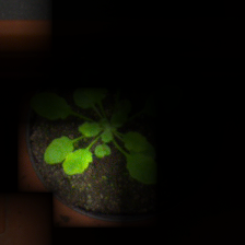
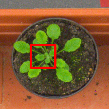
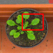
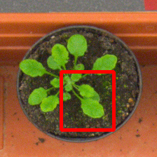
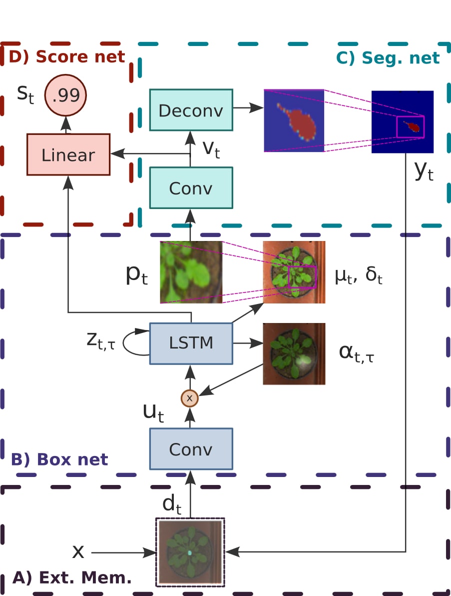
Our proposed model has four major components: A) an external memory that tracks the state of the segmented objects; B) a box proposal network responsible for localizing objects of interest; C) a segmentation network for segmenting image pixels within the box; and D) a scoring network that determines if an object instance has been found, and also decides when to stop. See Figure 2 for an illustration of these components.

Figure 2: Left: Detailed network design. Right: Sketch of training, and scheduled sampling; during training, the weighting of ground-truth instance segmentations relative to model predictions ($\theta_{t}$) decays to zero.

Notation. We use the following notation to describe the model architecture: $\textbf{x}_{0}\in\mathbb{R}^{H\times W\times C}$ is the input image ($H$, $W$ denotes the dimension, and $C$ denotes the color channel); $t$ indexes the iterations of the model, and $\tau$ indexes the glimpses of the box network’s inner RNN; $\textbf{y}=\{\textbf{y}_{t}|\textbf{y}_{t}\in[0,1]^{H\times W}\}_{t=1}^{T}$, $\textbf{y}^{*}=\{\textbf{y}^{*}_{t}|\textbf{y}^{*}_{t}\in\{0,1\}^{H\times W}\}_{t=1}^{T}$ are the output/ground-truth segmentation sequences; $\textbf{s}=\{s_{t}|s_{t}\in[0,1]\}_{t=1}^{T}$, $\textbf{s}^{*}=\{s^{*}_{t}|s^{*}_{t}\in\{0,1\}\}_{t=1}^{T}$ are the output/ground-truth confidence score sequences. $\textbf{h}=\text{CNN}(I)$ denotes passing an image $I$ through a CNN and returning the hidden activation h. $I^{\prime}=\text{D-CNN}(\textbf{h})$ denotes passing an activation map $h$ through a de-convolutional network (D-CNN) and returning an image $I^{\prime}$. $\textbf{h}_{t}=\text{LSTM}(\textbf{h}_{t-1},\textbf{x}_{t})$ denotes unrolling the long short-term memory (LSTM) by one time-step with the previous hidden state $\textbf{h}_{t-1}$ and current input $\textbf{x}_{t}$, and returning the current hidden state $\textbf{h}_{t}$. $\textbf{h}=\text{MLP}(\textbf{x})$ denotes passing an input x through a multi-layer perceptron (MLP) and returning the hidden state h.

Input pre-processing. We pre-train a FCN [27] to perform input pre-processing. This pre-trained FCN has two output components. The first is a 1-channel pixel-level foreground segmentation, produced by a variant of the DeconvNet [30] with skip connections. In addition to predicting this foreground mask, as a second component we followed the work of Uhrig et al. [41] by producing an angle map for each object. For each foreground pixel, we calculate its relative angle towards the centroid of the object, and quantize the angle into 8 different classes, forming 8 channels, as shown in Figure 3. Predicting the angle map forces the model to encode more detailed information about object boundaries. The architecture and training of these components are detailed in the Appendix. We denote $\textbf{x}_{0}$ as the original image (3 channel RGB), and x as the pre-processed image (9 channels: 1 for foreground and 8 for angles).

2.1 Part A: External memory

Figure 3: Illustration of the output of the pretrained FCN. Left: input image. Middle: predicted foreground. Right: predicted angle map.

To decide where to look next based on the already segmented objects, we incorporate an external memory, which provides object boundary details from all previous steps. We hypothesize that providing information of the completed segmentation helps the network reason about occluded objects and determine the next region of interest. The canvas has 10 channels in total: the first channel of the canvas keeps adding new pixels from the output of the previous time step, and the other channels store the input image.

$$\textbf{c}_{t}=\begin{cases}\textbf{0},&\text{if }t=0\\ \max(\textbf{c}_{t-1},\textbf{y}_{t-1}),&\text{otherwise}\end{cases}$$ (1)

$$\textbf{d}_{t}=\left[\textbf{c}_{t},\textbf{x}\right]$$ (2)

2.2 Part B: Box network

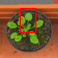
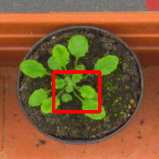
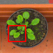
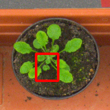
The box network plays a critical role, localizing the next object of interest. The CNN in the box network outputs a $H^{\prime}\times W^{\prime}\times L$ feature map $\textbf{u}_{t}$ ($H^{\prime}$ is the height; $W^{\prime}$ is the width; $L$ is the feature dimension). CNN activation based on the entire image is too complex and inefficient to process simultaneously. Simple pooling does not preserve location; instead we employ a “soft-attention” (dynamic pooling) mechanism here to extract useful information along spatial dimensions, weighted by $\alpha_{t}^{h,w}$. Since a single glimpse may not give the upper network enough information to decide where exactly to draw the box, we allow the glimpse LSTM to look at different locations by feeding a dimension $L$ vector each time. $\alpha$ is initialized to be uniform over all locations, and $\tau$ indexes the glimpses.

$$\textbf{u}_{t} =\text{CNN}(\textbf{d}_{t})$$ (3)

$$\textbf{z}_{t,\tau} =\begin{cases}\textbf{0},&\text{if }\tau=0\\ \text{LSTM}(\textbf{z}_{t,\tau-1},\sum\limits_{h,w}\alpha^{h,w}_{t,\tau-1}u^{h,w,l}_{t})&\text{otherwise}\end{cases}$$ (4)

$$\alpha_{t,\tau}^{h,w} =\begin{cases}1/(H^{\prime}\times W^{\prime}),&\text{if }\tau=0\\ \text{MLP}(\textbf{z}_{t,\tau}),&\text{otherwise}\end{cases}$$ (5)

We pass the LSTM’s hidden state through a linear layer to obtain predicted box coordinates. We parameterize the box by its normalized center $(\tilde{g}_{X},\tilde{g}_{Y})$, and size $(\log\tilde{\delta}_{X},\log\tilde{\delta}_{Y})$. A scaling factor $\gamma$ is also predicted by the linear layer, and used when re-projecting the patch to the original image size.

$$[\tilde{g}_{X,Y},\log\tilde{\delta}_{X,Y},\log\sigma_{X,Y},\gamma] =\textbf{w}_{b}^{\top}\textbf{z}_{t,\text{end}}+w_{b0}$$ (6)

$$g_{X} =(\tilde{g}_{X}+1)W/2$$ (7)

$$g_{Y} =(\tilde{g}_{Y}+1)H/2$$ (8)

$$\delta_{X} =\tilde{\delta}_{X}W$$ (9)

$$\delta_{Y} =\tilde{\delta}_{Y}H$$ (10)

Extracting a sub-region. We follow DRAW [16] and use a Gaussian interpolation kernel to extract an $\tilde{H}\times\tilde{W}$ patch from the $\tilde{x}$, a concatenation of the original image with $\textbf{d}_{t}$. We further allow the model to output rectangular patches to account for different shapes of the object. $i,j$ index the location in the patch of dimension $\tilde{H}\times\tilde{W}$, and $a,b$ index the location in the original image. $F_{X}$ and $F_{Y}$ are matrices of dimension $W\times\tilde{W}$ and $H\times\tilde{H}$, which indicates the contribution of the location $(a,b)$ in the original image towards the location $(i,j)$ in the extracted patch. $\mu_{X,Y}$ and $\sigma_{X,Y}$ are mean and variance of the Gaussian interpolation kernel, predicted by the box network.

$$\mu_{X}^{i} =g_{X}+(\delta_{X}+1)\cdot(i-\tilde{W}/2+0.5)/\tilde{W}$$ (11)

$$\mu_{Y}^{j} =g_{Y}+(\delta_{Y}+1)\cdot(j-\tilde{H}/2+0.5)/\tilde{H}$$ (12)

$$F_{X}^{a,i} =\frac{1}{\sqrt{2\pi}\sigma_{X}}\exp\left(-\frac{(a-\mu_{X}^{i})^{2}}{2\sigma_{X}^{2}}\right)$$ (13)

$$F_{Y}^{b,j} =\frac{1}{\sqrt{2\pi}\sigma_{Y}}\exp\left(-\frac{(b-\mu_{Y}^{j})^{2}}{2\sigma_{Y}^{2}}\right)$$ (14)

$$\tilde{\textbf{x}}_{t} =[\textbf{x}_{0},\textbf{d}_{t}]$$ (15)

$$\textbf{p}_{t} =\text{Extract}(\tilde{\textbf{x}}_{t},F_{Y},F_{X})\equiv F_{Y}^{\top}\tilde{\textbf{x}}_{t}F_{X}$$ (16)

2.3 Part C: Segmentation network

The remaining task is to segment out the pixels that belong to the dominant object within the window. The segmentation network first utilizes a convolution network to produce a feature map $\textbf{v}_{t}$. We then adopt a variant of the DeconvNet [30] with skip connections, which appends deconvolution (or convolution transpose) layers to upsample the low-resolution feature map to a full-size segmentation. After the fully convolutional layers we get a patch-level segmentation prediction heat map $\tilde{y}_{t}$. We then re-project this patch prediction to the original image using the transpose of the previously computed Gaussian filters; the learned $\gamma$ magnifies the signal within the bounding box, and a constant $\beta$ suppresses the pixels outside the box. Applying the sigmoid function produces segmentation values between 0 and 1.

$$\textbf{v}_{t} =\text{CNN}(\textbf{p}_{t})$$ (17)

$$\tilde{\textbf{y}}_{t} =\text{D-CNN}(\textbf{v}_{t})$$ (18)

$$\textbf{y}_{t} =\text{sigmoid}\left(\gamma\cdot\text{Extract}(\tilde{\textbf{y}}_{t},F_{Y}^{\top},F_{X}^{\top})-\beta\right)$$ (19)

2.4 Part D: Scoring network

To estimate the number of objects in the image, and to terminate our sequential process, we incorporate a scoring network, similar to the one presented in [36]. Our scoring network takes information from the hidden states of both the box network ($\textbf{z}_{t}$) and segmentation network ($\textbf{v}_{t}$) to produce a score between 0 and 1.

$$s_{t}=\text{sigmoid}(\textbf{w}_{zs}^{\top}\textbf{z}_{t,\text{end}}+\textbf{w}_{vs}^{\top}\textbf{v}_{t}+w_{s0})$$ (20)

Termination condition. We train the entire model with a sequence length determined by the maximum number of objects plus one. During inference, we cut off iterations once the output score goes below 0.5. The score loss function (described below) encourages scores to decrease monotonically.

2.5 Loss functions

Joint loss. The total loss function is a sum of three losses: the segmentation matching IoU loss $\mathcal{L}_{y}$; the box IoU loss $\mathcal{L}_{b}$; and the score cross-entropy loss $\mathcal{L}_{s}$:

$$\mathcal{L}(\textbf{y},\textbf{b},\textbf{s})=\mathcal{L}_{y}(\textbf{y},\textbf{y}^{*})+\lambda_{b}\mathcal{L}_{b}(\textbf{b},\textbf{b}^{*})+\lambda_{s}\mathcal{L}_{s}(\textbf{s},\textbf{s}^{*})$$ (21)

We fix the loss coefficients $\lambda_{b}$ and $\lambda_{s}$ to be 1 for all of our experiments.

(a) Matching IoU loss (mIOU). A primary challenge of instance segmentation involves matching model and ground-truth instances. We compute a maximum-weighted bipartite graph matching between the output instances and ground-truth instances (c.f., [40] and [36]). Matching makes the loss insensitive to the ordering of the ground-truth instances. Unlike coverage scores proposed in [39] it directly penalizes both false positive and false negative segmentations. The matching weight $\mathcal{M}_{i,j}$ is the IoU score between a pair of segmentations. We use the Hungarian algorithm to compute the matching; we do not back-propagate the network gradients through this algorithm.

$$\mathcal{M}_{i,j} =\text{softIOU}(\textbf{y}_{i},\textbf{y}^{*}_{j})\equiv\frac{\sum\textbf{y}_{i}\cdot\textbf{y}^{*}_{j}}{\sum\textbf{y}_{i}+\textbf{y}^{*}_{j}-\textbf{y}_{i}\cdot\textbf{y}^{*}_{j}}$$ (22)

$$\mathcal{L}_{y}(\textbf{y},\textbf{y}^{*}) =-\text{mIOU}(\textbf{y},\textbf{y}^{*})$$ (23)

$$\equiv-\frac{1}{N}\sum_{i,j}\mathcal{M}_{i,j}\mathbbm{1}[\text{match}(\textbf{y}_{i})=\textbf{y}^{*}_{j}]$$ (24)

(b) Soft box IoU loss. Although the exact IoU can be derived from the 4-d box coordinates, its gradient vanishes when two boxes do not overlap, which can be problematic for gradient-based learning. Instead, we propose a soft version of the box IoU. We use the same Gaussian filter to re-project a constant patch on the original image, pad the ground-truth boxes, and then compute the mIOU between the predicted box and the matched padded ground-truth bounding box that is scaled proportionally in both height and width.

$$\textbf{b}_{t} =\text{sigmoid}(\gamma\cdot\text{Extract}(\mathbf{1},F_{Y}^{\top},F_{X}^{\top})-\beta)$$ (25)

$$\mathcal{L}_{b}(\textbf{b},\textbf{b}^{*}) =-\text{mIOU}(\textbf{b},\text{Pad}(\textbf{b}^{*}))$$ (26)

(c) Monotonic score loss. To facilitate automatic termination, the network should output more confident objects first. We formulate a loss function that encourages monotonically decreasing values in the score output. Iterations with target score 1 are compared to the lower bound of preceding scores, and 0 targets to the upper bound of subsequent scores.

$$\begin{split}\mathcal{L}_{s}(\textbf{s},\textbf{s}^{*})=\frac{1}{T}\sum_{t}&-s^{*}_{t}\log\left(\min_{t^{\prime}\leq t}\{s_{t^{\prime}}\}\right)\\ &-(1-s^{*}_{t})\log\left(1-\max_{t^{\prime}\geq t}\{s_{t^{\prime}}\}\right)\end{split}$$ (27)

2.6 Training procedure

Bootstrap training. The box and segmentation networks rely on the output of each other to make decisions for the next time-step. Due to the coupled nature of the two networks, we propose a bootstrap training procedure: these networks are pre-trained with ground-truth segmentation and boxes, respectively, and in later stages we replace the ground-truth with the model predicted values.

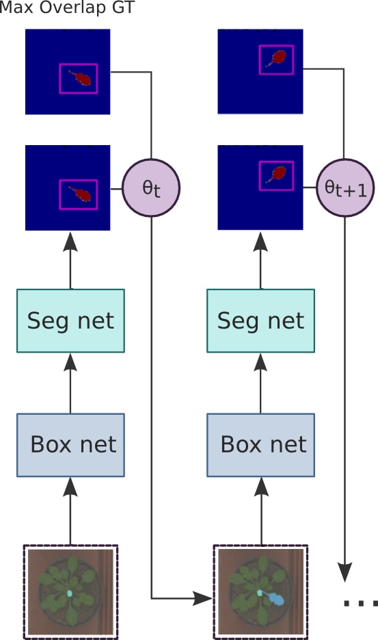
Scheduled sampling. To smooth out the transition between stages, we explore the idea of “scheduled sampling” [4], where we gradually remove the reliance on ground-truth segmentation at the input of the network. As shown in Figure 2, during training there is a stochastic switch ($\theta_{t}$) in the input of the external memory, to utilize either the maximally overlapping ground-truth instance segmentation, or the output of the network from the previous time step. By the end of the training, the model completely relies on its own output from the previous step, which matches the test-time inference procedure.

3 Related Work

Instance segmentation has recently received a burst of research attention, as it provides higher level of precision of image understanding compared to object detection and semantic segmentation.

Detector-based approaches. Early work on object segmentation [5] starts from a trained class detectors, which provide a bottom-up merging criterion based on top-down detections. [43] extends this approach with a DPM detector, and uses layered graphical models to reason about instance separation and occlusion. Besides boxes, models can also leverage region proposals and region descriptors [6]. Simultaneous detection and segmentation (SDS) methods [17, 18, 25, 24] apply newer CNN-based detectors such as RCNN [14], and perform segmentation using the bounding boxes as starting point. [24] proposes a trainable iterative refining procedure. Dai et al. [10] propose a pipeline-based approach which first predicts bounding box proposals and then performs segmentation within each ROI. Similarly, we jointly learn a detector and a segmentor; however, we introduce a direct feedback loop in the sequence of predictions. In addition, we learn the sequence ordering.

Graphical model approaches. Another line of research is to use generative graphical model to express the dependency structure among instances and pixels. Eslami et al. [11] proposes a restricted Boltzmann machine to capture high-order pixel interactions for shape modelling. A multi- stage pipeline proposed by Silberman et al. [39] is composed of patch-wise features based on deep learning, combined into a segmentation tree. More recently, Zhang et al. [45] formulate a dense CRF for instance segmentation; they apply a CNN on dense image patches to make local predictions, and construct a dense CRF to produce globally consistent labellings. Their key contribution is a shifting-label potential that encourages consistency across different patches. The graphical model formulation entails long running times, and their energy functions are dependent on instances being connected and having a clear depth ordering.

Fully convolutional approaches. Fully convolutional networks [27] has emerged as a powerful tool to directly predict dense pixel labellings. Pinheiro et al.  [33, 34] train a CNN to generate object segmentation proposals, which runs densely on all windows at multiple scales, a nd Dai et al. [9] uses relative location as additional pixel labels. The output of both systems are object proposals, which require further processing to get final segmentations. Other approaches using FCNs are proposal-free, but rely on a bottom-up merging process. Liang et al. [26] predict dense pixel prediction of object location and size, using clustering as a post-processing step. Uhrig et al.  [41] present another approach based on FCNs, which is trained to produces a semantic segmentation as well as an instance-aware angle map, encoding the instance centroids. Post-processing based on template matching and instance fusion produces the instance identities. Importantly, they also used ground-truth depth labels in training. Concurrent work [2, 19, 22] also explores a similar idea of using FCNs to output instance-sensitive embeddings.

RNN approaches. Another recent line of research, e.g., [40, 32, 36] employs end-to-end recurrent neural networks (RNN) to perform object detection and segmentation. The sequential decomposition idea for structured prediction is also explored in [20, 3]. A permutation agnostic loss function based on maximum weighted bipartite matching was proposed by [40]. To process an entire image, they treat each element of a CNN feature map individually. Similarly, our box proposal network also uses an RNN to generate box proposals: instead of running hundreds of RNN iterations, we only run it for a small number of iterations using a soft attention mechanism [42]. Romera-Paredes and Torr [36] use convolutional LSTM (ConvLSTM) [38] to produce instance segmentation directly. However, since their ConvLSTM is required to handle object detection, inhibition, and segmentation all convolutionally on a global scale, and it is hard for their model to inhibit far apart instances. In contrast, our architecture incorporates direct feedback from the prediction of the previous instance, providing precise boundary inhibition, and our box network confines the instance-wise segmentation within a local window.

4 Experiments

We refer readers to the Appendix for hyper-parameters and other training details of the experiments .

4.1 Datasets & Evaluation

CVPPP leaf segmentation. One instance segmentation benchmark is the CVPPP plant leaf dataset [28], which was developed due to the importance of instance segmentation in plant phenotyping. We ran the A1 subset of CVPPP plant leaf segmentation dataset. We trained our model on 128 labeled images, and report results on the 33 test images. We compare our performance to [36], and other top approaches that were published with the CVPPP conference; see the collation study [37] for details of these other approaches.

Image	GT	Ours		Image	GT	Ours

Sequence color legend:

Figure 4: Examples of our instance segmentation output on CVPPP leaf dataset. In this paper, instance colors are determined by the order of the model output sequence.

Image	GT	Ours		Image	GT	Ours

Figure 5: Examples of our instance segmentation output on MS-COCO zebra images.

KITTI car segmentation. Instance segmentation also provides rich information in the context of autonomous driving. Following [46, 45, 41], we also evaluated the model performance on the KITTI car segmentation dataset. We trained the model with 3,712 training images, and report performance on 120 validation images and 144 test images.

Cityscapes. Cityscapes provides multi-class instance-level annotation and is currently the most comprehensive benchmark for instance segmentation, containing 2,975 training images, 500 validation images, and 1,525 test images, with 8 semantic classes (person, rider, car, truck, bus, train, motorcycle, bicycle). We train our instance segmentation network as a class-agnostic model for all classes, and apply a semantic segmentation mask obtained from [13] on top of our instance output. Since “car” is the most common class, we report both average score on all classes, and individual score on the “car” class.

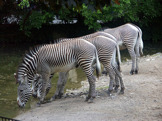
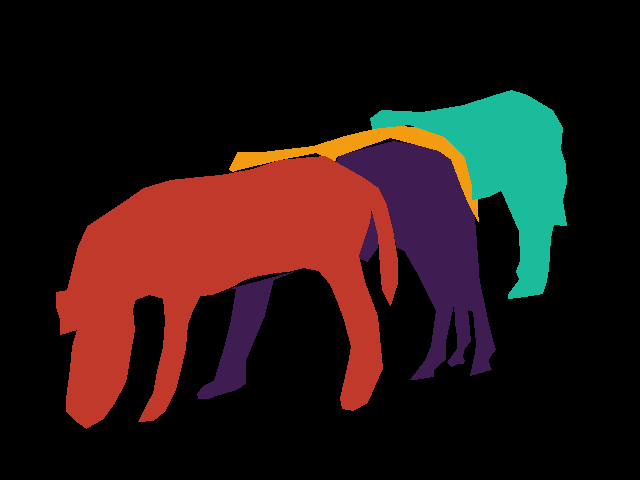
MS-COCO. To test the effectiveness and portability of our algorithm, we train our model on a subset of MS-COCO. As an initial study we select images of zebras, and train on 1000 images. Since there are no methods that are directly comparable, we leave the quantatitive results for Appendix.

Ablation studies. We also examine the relative importance of model components via ablation studies, and report validation performance on the KITTI dataset.

• No pre-processing. This network is trained to take as input raw image pixels, without the foreground segmentation or the angle map.

• No box net. Instead of predicting segmentation within a box, the output dimension of the segmentation network is the full image.

• No angles. The pre-processor predicts the foreground segmentation only, without the angle map.

• No scheduled sampling. This network has the same architecture but trained without scheduled sampling (see Section 2.6), i.e., at training time, always use the maximum overlapped ground-truth.

• Fewer iterations. The box network has fewer glimpses on the convnet feature map (fewer LSTM iterations).

Table 1: Leaf segmentation and counting performance, averaged over all test images, with standard deviation in parentheses

	SBD $\uparrow$	$|\text{DiC}|$ $\downarrow$
RIS+CRF [36]	66.6 (8.7)	1.1 (0.9)
MSU [37]	66.7 (7.6)	2.3 (1.6)
Nottingham [37]	68.3 (6.3)	3.8 (2.0)
Wageningen [44]	71.1 (6.2)	2.2 (1.6)
IPK [31]	74.4 (4.3)	2.6 (1.8)
PRIAn [15]	-	1.3(1.2)
Ours	84.9 (4.8)	0.8 (1.0)

Table 2: KITTI vehicle segmentation results

	Set	MWCov	MUCov	AvgFP	AvgFN
DepthOrder [46]	test	70.9	52.2	0.597	0.736
DenseCRF [45]	test	74.1	55.2	0.417	0.833
AngleFCN+Depth [41]	test	79.7	75.8	0.201	0.159
Ours	test	80.0	66.9	0.764	0.201

Evaluation metrics. We evaluate based on the metrics used by the other studies in the respective benchmarks. See Appendix for detailed equations for these metrics.

For segmentation, symmetric best dice (SBD) is used for leaves. (see Equations 28, 30).

$$\text{DICE}(A,B) =\frac{2|A\hat{B}|}{|A|+|B|}$$ (28)

$$\text{BD}(\{A_{i}\},B) =\max_{i}\text{DICE}(A_{i},B)$$ (29)

$$\begin{split}\text{SBD}(y_{i}\},\{y^{*}_{j}\})=\min(&\frac{1}{N}\sum_{j}\text{BD}(\{y_{i}\},y^{*}_{j}),\\ &\frac{1}{M}\sum_{i}\text{BD}(\{y^{*}_{j}\},y_{i}))\end{split}$$ (30)

Mean (weighted) coverage (MWCov, MUCov) are used for KITTI car segmentation. (see Equations 32, 31). The coverage scores measure the instance-wise IoU for each ground-truth instance averaged over the image; MWCov further weights the score by the size of the ground-truth instance segmentation (larger objects get larger weights).

$$\text{MUCov}(\{y_{i}\},\{y_{j}^{*}\}) =\sum_{i}\frac{1}{N}\max_{j}\text{IoU}(y_{i},y_{j}^{*})$$ (31)

$$\text{MWCov}(\{y_{i}\},\{y_{j}^{*}\}) =\sum_{i}w_{\text{cov},i}\max_{j}\text{IoU}(y_{i},y_{j}^{*})$$ (32)

$$w_{\text{cov},i} =\frac{|y_{i}|}{\sum_{i}|y_{i}|}$$ (33)

The Cityscapes evaluation uses average precision (AP), (see Equation 34), which counts the precision between a pair of matched prediction and groundtruth, for a range of IoU threshold values.

$$\begin{split}\text{AP}(\{y_{i}\},\{y_{j}^{*}\})=&\max_{s}\sum_{\theta}\sum_{j}Pr(y_{s(i)},y_{j})\cdot\\ &\mathbbm{1}[\text{IoU}(y_{s(i)},y^{*}_{j})\geq\theta],\end{split}$$ (34)

where $s$ is a function that permutes the predicted instance order, and $\theta$ is the threshold from 0.5 to 0.95. Other scores include AP${}^{\text{50\%}}$ for a threshold of $0.5$, and AP${}^{\text{50m, 100m}}$ for a subset of instances within 50m and 100m.

Counting is measured in absolute difference in count ($|\text{DiC}|$) (i.e., mean absolute error), (see Equation 35), average false positive (AvgFP), and average false negative (AvgFN). False positive is the number of predicted instances that do not overlap with the ground-truth, and false negative is the number of ground-truth instances that do not overlap with the prediction.

$$|\text{DiC}|=\frac{1}{N}\sum_{i}|count_{i}-count_{i}^{*}|$$ (35)

Table 3: Cityscapes instance-level segmentation results

	Set	AP	AP${}^{\text{50\%}}$	AP${}^{\text{50m}}$	AP${}^{\text{100m}}$
MCG+RCNN [8]	all	4.6	12.9	7.7	10.3
AngleFCN+Depth [41]	all	8.9	21.1	15.3	16.7
Ours	all	9.5	18.9	16.8	20.9
MCG+RCNN [8]	car	10.5	26.0	17.5	21.2
AngleFCN+Depth [41]	car	22.5	37.8	36.4	40.7
Ours	car	27.5	41.9	46.8	54.2

Table 4: Ablation results on KITTI validation

	Set	MWCov	MUCov	AvgFP	AvgFN
No Pre Proc.	val	55.6	45.0	0.125	0.417
No Box Net	val	57.0	49.1	0.757	0.375
No Angle	val	71.2	63.3	0.542	0.342
No Sched. Samp.	val	73.6	63.9	0.350	0.317
Iter-1	val	64.1	54.8	0.200	0.375
Iter-3	val	71.3	63.4	0.417	0.308
Full (Iter-5)	val	75.1	64.6	0.375	0.283

Image		GT		Ours

Figure 6: Examples of our instance segmentation output on Cityscapes (row 1-3) and KITTI (row 4-5).

4.2 Results & Discussion

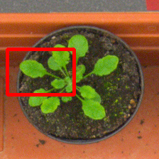
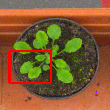
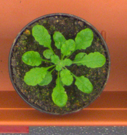
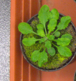
Example results on the leaf segmentation task are shown in Figure 4. On this task, our best model outperforms the previous state-of-the-art by a large margin in both segmentation and counting (see Table 1). In particular, our method has significant improvement over a previous RNN-based instance segmentation method [36]. We found that our model with the FCN pre-processor overfit on this task, and we thus utilized the simpler version without input pre-processing. This is not surprising, as the dataset is very small, and including the FCN significantly increases the input dimension and number of parameters.

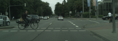
On the KITTI task, Figure 6 row 4-5 shows that our model can segment cars in a wide variety of poses. Our method out-performs [46, 45], but scores lower than [41] (see Table 2). One possible explanation is their inclusion of depth information during training, which may help the model disambiguate distant object boundaries. Moreover, their bottom-up “instance fusion” method plays a crucial role (omitting this leads to a steep performance drop); this likely helps segment smaller objects, whereas our box network does not reliably detect distant cars.

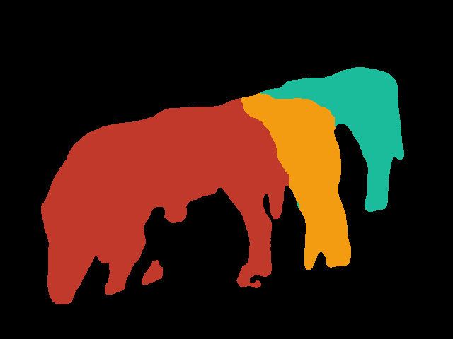
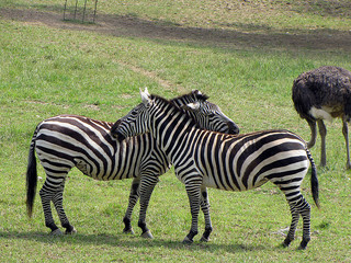
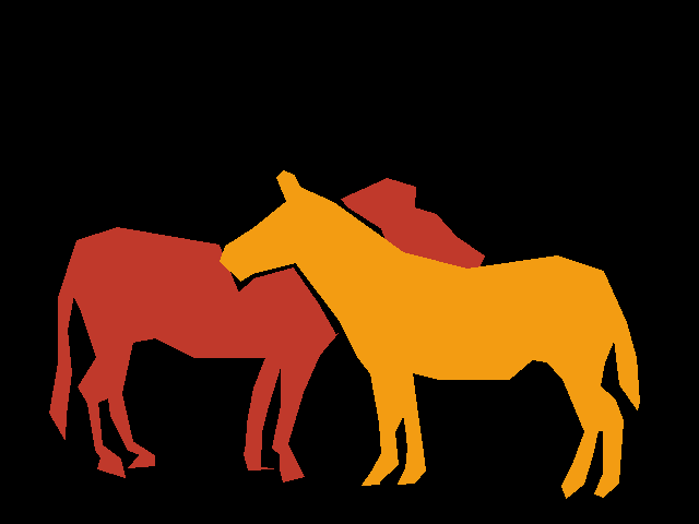
The displayed segmentations demonstrate that our top-down attentional inference is crucial for a good instance recognition model. This allows disconnected components belonging to objects such as a bicycle (Figure 6 row 2) to be recognized as a whole piece whereas [45] models the connectedness as their energy potential. Our model also shows impressive results in heavily occluded scenes, when only small proportion of the car is visible (Figure 6 row 1), and when the zebra in the back reveals two disjoint pieces of its body (Figure 5 right). Another advantage is that our model directly outputs the final segmentation, eliminating the need for post- processing, which is often required by other methods (e.g. [26, 41]).

Our method also learns to rank the importance of instances through visual attention. During training, the model first attended to objects in a spatial ordering (e.g. left to right), and then gradually shifted to a more sophisticated ordering based on confidence, with larger attentional jumps in between timesteps.

Some failure cases of our approach, e.g., omitting distant objects and under- segmentation, may be explained by our downsampling factor; to manage training time, we down-sample KITTI and Cityscapes by a factor around 4, whereas [41] does not do any any downsampling. We also observe a lack of higher-order reasoning, e.g., the inclusion of the “third” limb of a person in the bottom of Figure 6. As future work, these problems can be addressed by a combination of our method with bottom-up merging methods (e.g. [26, 41]) and higher order graphical models (e.g. [29, 11]).

Finally, our ablation studies (see Table 4) help elucidate the contribution of some model components. The initial foreground segmentation, and the box network both play crucial roles , as seen in the coverage measures. Scheduled sampling results in slightly better performance, by making training resemble testing, gradually forcing the model to carry out a full sequence. Larger numbers of glimpses of the LSTM (Iter-$n$) helps the model significantly by allowing more information to be considered before outputting the next region of interest. Finally, we note that KITTI has a fairly small validation and test set, so these results are highly variable (see last lines of Table 4 versus Table 2).

5 Conclusion

In this work, we borrow intuition from human counting and formulate instance segmentation as a recurrent attentive process. Our end-to-end recurrent architecture demonstrates significant improvement compared to earlier formulations using RNN on the same tasks, and shows state-of-the-art results on challenging instance segmentation datasets. We address the classic object occlusion problem with an external memory, and the attention mechanism permits segmentation at a fine resolution.

Our attentional architecture significantly reduces the number of parameters, and the performance is quite strong despite being trained with only 100 leaf images and under 3,000 road scene images. Since our model is end-to-end trainable and does not depend on prior knowledge of the object type (e.g. size, connectedness), we expect our method performance to scale directly with the number of labelled images, which is certain to increase as this task gains in popularity and new datasets become available. As future work, we are currently extending our model to tackle highly multi-class instance segmentation, such as the MS-COCO dataset, and more structured understanding of everyday scenes.

Acknowledgements

Supported by Samsung and the Intelligence Advanced Research Projects Activity (IARPA) via Department of Interior/Interior Business Center (DoI/IBC) contract number D16PC00003. The U.S. Government is authorized to reproduce and distribute reprints for Governmental purposes notwithstanding any copyright annotation thereon. Disclaimer: The views and conclusions contained herein are those of the authors and should not be interpreted as necessarily representing the official policies or endorsements, either expressed or implied, of IARPA, DoI/IBC, or the U.S. Government.

Appendix A Training procedure specification

We used the Adam optimizer [21] with learning rate 0.001 and batch size of 8. The learning rate is multiplied by 0.85 for every 5000 steps of training.

A.1 Scheduled sampling

We denote $\theta_{t}$ as the probability of feeding in ground-truth segmentation that has the greatest overlap with the previous prediction, as opposed to model output. $\theta_{t}$ decays exponentially as training proceeds, and for larger $t$, the decay occurs later:

$$\theta_{t} =\min\left(\Gamma_{t}\exp\left(-\frac{epoch-S}{S_{2}}\right),1\right)$$ (36)

$$\Gamma_{t} =1+\log(1+Kt)$$ (37)

where $epoch$ is the training index, $S$, $S_{2}$, and $K$ are constants. In the experiments reported here, these values are $10000$, $2885$, and $3$.

Appendix B More experimental results

We include the segmentation and counting performance on the MS-COCO zebra images in Table 5. In terms of counting, our model out-performs a baseline method that runs an object detector and then non-maximal suppression, and a new associative-subitizing method  [7].

Table 5: MS-COCO Zebra Results

	MWCov $\uparrow$	MUCov $\uparrow$	$|$DiC$|$ $\downarrow$	Acc. $\uparrow$
detect [7]	-	-	2.56	-
aso-sub [7]	-	-	1.03	-
Ours	69.2	64.2	0.79	0.57

Appendix C Model architecture

C.1 Foreground + Orientation FCN

We resize the image to uniform size. For CVPPP and MS-COCO dataset, we adopt a uniform size of $224\times 224$, for KITTI, we adopt $128\times 448$, and for Cityscapes $256\times 512$ (4x downsampling). Table 6 lists the specification of all layers.

Table 6: FCN specification

Name	Type	Input	Spec (size/stride)	Size CVPPP/MS-COCO	Size KITTI	Size Cityscapes
input	input	-	-	$224\times 224\times 3$	$128\times 448\times 3$	$256\times 512\times 3$
conv1-1	conv	input	$3\times 3\times 3\times 32$	$224\times 224\times 32$	$128\times 448\times 64$	$256\times 512\times 64$
conv1-2	conv	conv1-1	$3\times 3\times 32\times 64$	$224\times 224\times 64$	$128\times 448\times 32$	$256\times 512\times 32$
pool1	pool	conv1-2	max $2\times 2$	$112\times 112\times 64$	$64\times 224\times 64$	$128\times 256\times 64$
conv2-1	conv	pool1	$3\times 3\times 64\times 64$	$112\times 112\times 64$	$64\times 224\times 64$	$128\times 256\times 64$
conv2-2	conv	conv2-1	$3\times 3\times 64\times 96$	$112\times 112\times 96$	$64\times 224\times 96$	$128\times 256\times 96$
pool2	pool	conv2-2	max $2\times 2$	$56\times 56\times 96$	$32\times 112\times 96$	$64\times 128\times 96$
conv3-1	conv	pool2	$3\times 3\times 96\times 96$	$56\times 56\times 96$	$32\times 112\times 96$	$64\times 128\times 96$
conv3-2	conv	conv3-1	$3\times 3\times 96\times 128$	$56\times 56\times 128$	$32\times 112\times 128$	$64\times 128\times 128$
pool3	pool	conv3-2	max $2\times 2$	$28\times 28\times 128$	$16\times 56\times 128$	$32\times 64\times 128$
conv4-1	conv	pool3	$3\times 3\times 128\times 128$	$28\times 28\times 128$	$16\times 56\times 128$	$32\times 64\times 128$
conv4-2	conv	conv4-1	$3\times 3\times 128\times 128$	$28\times 28\times 128$	$16\times 56\times 128$	$32\times 64\times 128$
conv4-3	conv	conv4-2	$3\times 3\times 128\times 128$	$28\times 28\times 128$	$16\times 56\times 128$	$32\times 64\times 128$
conv4-4	conv	conv4-3	$3\times 3\times 128\times 128$	$28\times 28\times 128$	$16\times 56\times 128$	$32\times 64\times 128$
conv4-5	conv	conv4-4	$3\times 3\times 128\times 128$	$28\times 28\times 128$	$16\times 56\times 128$	$32\times 64\times 128$
conv4-6	conv	conv4-5	$3\times 3\times 128\times 128$	$28\times 28\times 128$	$16\times 56\times 128$	$32\times 64\times 128$
conv4-7	conv	conv4-6	$3\times 3\times 128\times 128$	$28\times 28\times 128$	$16\times 56\times 128$	$32\times 64\times 128$
conv4-8	conv	conv4-7	$3\times 3\times 128\times 256$	$28\times 28\times 256$	$16\times 56\times 256$	$32\times 64\times 256$
pool4	pool	conv4-8	max $2\times 2$	$14\times 14\times 256$	$8\times 28\times 256$	$16\times 32\times 256$
conv5-1	conv	pool4	$3\times 3\times 256\times 256$	$14\times 14\times 256$	$8\times 28\times 256$	$16\times 32\times 256$
conv5-2	conv	conv5-1	$3\times 3\times 256\times 256$	$14\times 14\times 256$	$8\times 28\times 256$	$16\times 32\times 256$
conv5-3	conv	conv5-2	$3\times 3\times 256\times 256$	$14\times 14\times 256$	$8\times 28\times 256$	$16\times 32\times 256$
conv5-4	conv	conv5-3	$3\times 3\times 256\times 512$	$14\times 14\times 512$	$8\times 28\times 512$	$16\times 32\times 512$
pool5	pool	conv5-4	max $2\times 2$	$7\times 7\times 512$	$4\times 14\times 512$	$8\times 16\times 512$
deconv6-1	deconv	pool5	$3\times 3\times 256\times 512/2$	$14\times 14\times 256$	$8\times 28\times 256$	$16\times 32\times 256$
deconv6-2	deconv	deconv6-1 + conv5-3	$3\times 3\times 256\times 512$	$14\times 14\times 256$	$8\times 28\times 256$	$16\times 32\times 256$
deconv7-1	deconv	deconv6-2	$3\times 3\times 128\times 256/2$	$28\times 28\times 128$	$16\times 56\times 128$	$32\times 64\times 128$
deconv7-2	deconv	deconv7-1 + conv4-7	$3\times 3\times 128\times 256$	$28\times 28\times 128$	$16\times 56\times 128$	$32\times 64\times 128$
deconv8-1	deconv	deconv7-2	$3\times 3\times 96\times 128/2$	$56\times 56\times 96$	$32\times 112\times 96$	$64\times 128\times 96$
deconv8-2	deconv	deconv8-1 + conv3-1	$3\times 3\times 96\times 192$	$56\times 56\times 96$	$32\times 112\times 96$	$64\times 128\times 96$
deconv9-1	deconv	deconv8-2	$3\times 3\times 64\times 96/2$	$112\times 112\times 64$	$64\times 224\times 64$	$128\times 256\times 64$
deconv9-2	deconv	deconv9-1	$3\times 3\times 64\times 64$	$112\times 112\times 64$	$64\times 224\times 64$	$128\times 256\times 64$
deconv10-1	deconv	deconv9-2	$3\times 3\times 32\times 64/2$	$224\times 224\times 32$	$128\times 448\times 32$	$256\times 512\times 32$
deconv10-2	deconv	deconv10-1	$3\times 3\times 32\times 32$	$224\times 224\times 32$	$128\times 448\times 32$	$256\times 512\times 32$
deconv10-3	deconv	deconv10-2 + input	$3\times 3\times 9\times 35$	$224\times 224\times 9$	$128\times 448\times 9$	$256\times 512\times 9$

C.2 External memory

Table 7: External memory specification

Name	Filter spec	Size CVPPP/MS-COCO	Size KITTI	Size Cityscapes
ConvLSTM	$3\times 3$	$224\times 224\times 9$	$128\times 448\times 9$	$256\times 512\times 9$

C.3 Box network

The box network takes in 9 channels of input directly from the output of the FCN. It goes through a CNN structure again and uses the attention vector predicted by the LSTM to perform dynamic pooling in the last layer. The CNN hyperparameters are listed in Table 8 and the LSTM and glimpse MLP hyperparameters are listed in Table 9. The glimpse MLP takes input from the hidden state of the LSTM and outputs a vector of normalized weighting over all the box CNN feature map spatial grids.

Table 8: Box network CNN specification

Name	Type	Input	Spec (size/stride)	Size CVPPP/MS-COCO	Size KITTI	Size Cityscapes
input	input	-	-	$224\times 224\times 9$	$128\times 448\times 9$	$256\times 512\times 9$
conv1-1	conv	input	$3\times 3\times 9\times 16$	$224\times 224\times 16$	$128\times 448\times 16$	$256\times 512\times 16$
pool1	pool	conv1-2	max $2\times 2$	$112\times 112\times 16$	$64\times 224\times 16$	$128\times 256\times 16$
conv1-2	conv	conv1-1	$3\times 3\times 16\times 16$	$112\times 112\times 16$	$64\times 224\times 16$	$128\times 256\times 16$
pool1	pool	conv1-2	max $2\times 2$	$56\times 56\times 16$	$32\times 112\times 16$	$64\times 128\times 16$
conv2-1	conv	pool1	$3\times 3\times 16\times 32$	$56\times 56\times 32$	$32\times 112\times 32$	$64\times 128\times 32$
conv2-2	conv	conv2-1	$3\times 3\times 32\times 32$	$56\times 56\times 32$	$32\times 112\times 32$	$64\times 128\times 32$
pool2	pool	conv2-2	max $2\times 2$	$28\times 28\times 32$	$16\times 56\times 32$	$32\times 64\times 32$
conv3-1	conv	pool2	$3\times 3\times 32\times 64$	$28\times 28\times 64$	$16\times 56\times 64$	$32\times 64\times 64$
conv3-2	conv	conv3-1	$3\times 3\times 64\times 64$	$28\times 28\times 64$	$16\times 56\times 64$	$32\times 64\times 64$
pool3	pool	conv3-2	max $2\times 2$	$14\times 14\times 64$	$8\times 28\times 64$	$16\times 32\times 64$
conv3-1	conv	pool2	$3\times 3\times 64\times 64$	$14\times 14\times 64$	$8\times 28\times 64$	$16\times 32\times 64$
conv3-2	conv	conv3-1	$3\times 3\times 64\times 64$	$14\times 14\times 64$	$8\times 28\times 64$	$16\times 32\times 64$
pool3	pool	conv3-2	max $2\times 2$	$7\times 7\times 64$	$4\times 14\times 64$	$8\times 16\times 64$

Table 9: Box network LSTM specification

Name	Size CVPPP/MS-COCO	Size KITTI	Size Cityscapes
LSTM	$256$	$256$	$256$
GlimpseMLP1	$256$	$256$	$256$
GlimpseMLP2	$7\times 7$	$4\times 14$	$8\times 16$

C.4 Segmentation network

The segmentation networks takes in a patch of size $48\times 48$ with multiple channels. The first three channels are the original image R, G, B channels. Then there are 8 channels of orientation angles, and then 1 channel of foreground heat map, all predicted by FCN. Full details are listed in Table 10. Constant $\beta$ is chosen to be 5.

Table 10: Segmentation network specification

Name	Type	Input	Spec (size/stride)	Size
input	input	-	-	$48\times 48\times 13$
conv1-1	conv	input	$3\times 3\times 13\times 16$	$48\times 48\times 16$
conv1-2	conv	conv1-1	$3\times 3\times 16\times 32$	$48\times 48\times 32$
pool1	pool	conv1-2	max $2\times 2$	$24\times 24\times 32$
conv2-1	conv	pool1	$3\times 3\times 32\times 32$	$24\times 24\times 32$
conv2-2	conv	conv2-1	$3\times 3\times 32\times 64$	$24\times 24\times 64$
pool3	pool	conv2-2	max $2\times 2$	$12\times 12\times 64$
conv3-1	conv	pool2	$3\times 3\times 64\times 64$	$12\times 12\times 64$
conv3-2	conv	conv3-1	$3\times 3\times 64\times 96$	$12\times 12\times 96$
pool3	pool	conv3-2	max $2\times 2$	$6\times 6\times 96$
deconv4-1	deconv	pool3	$3\times 3\times 64\times 96/2$	$12\times 12\times 64$
deconv4-2	deconv	deconv4-1 + conv3-1	$3\times 3\times 64\times 128$	$12\times 12\times 64$
deconv5-1	deconv	deconv4-2 + conv2-2	$3\times 3\times 32\times 128/2$	$24\times 24\times 32$
deconv5-2	deconv	deconv5-1 + conv2-1	$3\times 3\times 32\times 64$	$24\times 24\times 32$
deconv6-1	deconv	deconv5-2 + conv1-2	$3\times 3\times 16\times 64/2$	$48\times 48\times 16$
deconv6-2	deconv	deconv6-1 + conv1-1	$3\times 3\times 16\times 32$	$48\times 48\times 16$
deconv6-3	deconv	deconv6-2 + input	$3\times 3\times 1\times 29$	$48\times 48\times 1$

References

- [1] S. Antol, A. Agrawal, J. Lu, M. Mitchell, D. Batra, C. L. Zitnick, and D. Parikh. VQA: Visual question answering. In ICCV, 2015.
- [2] M. Bai and R. Urtasun. Deep watershed transform for instance segmentation. CoRR, abs/1611.08303, 2016.
- [3] D. Banica and C. Sminchisescu. Second-order constrained parametric proposals and sequential search-based structured prediction for semantic segmentation in RGB-D images. In CVPR, 2015.
- [4] S. Bengio, O. Vinyals, N. Jaitly, and N. Shazeer. Scheduled sampling for sequence prediction with recurrent neural networks. In NIPS, 2015.
- [5] E. Borenstein and S. Ullman. Class-specific, top-down segmentation. In ECCV, 2002.
- [6] J. Carreira, R. Caseiro, J. Batista, and C. Sminchisescu. Free-form region description with second-order pooling. TPAMI, 37(6):1177–1189, 2015.
- [7] P. Chattopadhyay, R. Vedantam, R. S. Ramprasaath, D. Batra, and D. Parikh. Counting everyday objects in everyday scenes. CoRR, abs/1604.03505, 2016.
- [8] M. Cordts, M. Omran, S. Ramos, T. Rehfeld, M. Enzweiler, R. Benenson, U. Franke, S. Roth, and B. Schiele. The cityscapes dataset for semantic urban scene understanding. CoRR, abs/1604.01685, 2016.
- [9] J. Dai, K. He, Y. Li, S. Ren, and J. Sun. Instance-sensitive fully convolutional networks. In ECCV, 2016.
- [10] J. Dai, K. He, and J. Sun. Instance-aware semantic segmentation via multi-task network cascades. CoRR, abs/1512.04412, 2015.
- [11] S. M. A. Eslami, N. Heess, C. K. I. Williams, and J. M. Winn. The shape boltzmann machine: A strong model of object shape. IJCV, 107(2):155–176, 2014.
- [12] A. Geiger, P. Lenz, and R. Urtasun. Are we ready for autonomous driving? The KITTI vision benchmark suite. In CVPR, 2012.
- [13] G. Ghiasi and C. C. Fowlkes. Laplacian pyramid reconstruction and refinement for semantic segmentation. In ECCV, 2016.
- [14] R. B. Girshick, J. Donahue, T. Darrell, and J. Malik. Rich feature hierarchies for accurate object detection and semantic segmentation. In CVPR, 2014.
- [15] M. V. Giuffrida, M. Minervini, and S. Tsaftaris. Learning to count leaves in rosette plants. In Proceedings of the Computer Vision Problems in Plant Phenotyping (CVPPP), 2015.
- [16] K. Gregor, I. Danihelka, A. Graves, D. J. Rezende, and D. Wierstra. DRAW: A recurrent neural network for image generation. In ICML, 2015.
- [17] B. Hariharan, P. A. Arbeláez, R. B. Girshick, and J. Malik. Simultaneous detection and segmentation. In ECCV, 2014.
- [18] B. Hariharan, P. A. Arbeláez, R. B. Girshick, and J. Malik. Hypercolumns for object segmentation and fine-grained localization. In CVPR, 2015.
- [19] Z. Hayder, X. He, and M. Salzmann. Shape-aware instance segmentation. CoRR, abs/1612.03129, 2016.
- [20] H. D. III, J. Langford, and D. Marcu. Search-based structured prediction. Machine Learning, 75(3):297–325, 2009.
- [21] D. P. Kingma and J. Ba. Adam: A method for stochastic optimization. In ICLR, 2015.
- [22] A. Kirillov, E. Levinkov, B. Andres, B. Savchynskyy, and C. Rother. InstanceCut: from edges to instances with multicut. CoRR, abs/1611.08272.
- [23] V. S. Lempitsky and A. Zisserman. Learning to count objects in images. In NIPS, 2010.
- [24] K. Li, B. Hariharan, and J. Malik. Iterative instance segmentation. In CVPR, 2016.
- [25] X. Liang, Y. Wei, X. Shen, Z. Jie, J. Feng, L. Lin, and S. Yan. Reversible recursive instance-level object segmentation. In CVPR, 2016.
- [26] X. Liang, Y. Wei, X. Shen, J. Yang, L. Lin, and S. Yan. Proposal-free network for instance-level object segmentation. CoRR, abs/1509.02636, 2015.
- [27] J. Long, E. Shelhamer, and T. Darrell. Fully convolutional networks for semantic segmentation. In CVPR, 2015.
- [28] M. Minervini, A. Fischbach, H. Scharr, and S. A. Tsaftaris. Finely-grained annotated datasets for image-based plant phenotyping. Pattern Recognition Letters, 2015. Special Issue on Fine-grained Categorization in Ecological Multimedia.
- [29] V. C. Nguyen, N. Ye, W. S. Lee, and H. L. Chieu. Conditional random field with high-order dependencies for sequence labeling and segmentation. JMLR, 15(1):981–1009, 2014.
- [30] H. Noh, S. Hong, and B. Han. Learning deconvolution network for semantic segmentation. In ICCV, 2015.
- [31] J. Pape and C. Klukas. 3-d histogram-based segmentation and leaf detection for rosette plants. In ECCV Workshops, 2014.
- [32] E. Park and A. C. Berg. Learning to decompose for object detection and instance segmentation. In ICLR Workshop, 2016.
- [33] P. H. O. Pinheiro, R. Collobert, and P. Dollár. Learning to segment object candidates. In NIPS, 2015.
- [34] P. O. Pinheiro, T. Lin, R. Collobert, and P. Dollár. Learning to refine object segments. In ECCV, pages 75–91, 2016.
- [35] M. Ren, R. Kiros, and R. S. Zemel. Exploring models and data for image question answering. In NIPS, 2015.
- [36] B. Romera-Paredes and P. H. S. Torr. Recurrent instance segmentation. CoRR, abs/1511.08250, 2015.
- [37] H. Scharr, M. Minervini, A. P. French, C. Klukas, D. M. Kramer, X. Liu, I. Luengo, J. Pape, G. Polder, D. Vukadinovic, X. Yin, and S. A. Tsaftaris. Leaf segmentation in plant phenotyping: A collation study. Mach. Vis. Appl., 27(4):585–606, 2016.
- [38] X. Shi, Z. Chen, H. Wang, D. Yeung, W. Wong, and W. Woo. Convolutional LSTM network: A machine learning approach for precipitation nowcasting. In NIPS, 2015.
- [39] N. Silberman, D. Sontag, and R. Fergus. Instance segmentation of indoor scenes using a coverage loss. In ECCV, 2014.
- [40] R. Stewart and M. Andriluka. End-to-end people detection in crowded scenes. CoRR, abs/1506.04878, 2016.
- [41] J. Uhrig, M. Cordts, U. Franke, and T. Brox. Pixel-level encoding and depth layering for instance-level semantic labeling. In GCPR, 2016.
- [42] K. Xu, J. Ba, R. Kiros, K. Cho, A. C. Courville, R. Salakhutdinov, R. S. Zemel, and Y. Bengio. Show, attend and tell: Neural image caption generation with visual attention. In ICML, 2015.
- [43] Y. Yang, S. Hallman, D. Ramanan, and C. C. Fowlkes. Layered object models for image segmentation. TPAMI, 34(9):1731–1743, 2012.
- [44] X. Yin, X. Liu, J. Chen, and D. M. Kramer. Multi-leaf tracking from fluorescence plant videos. In ICIP, 2014.
- [45] Z. Zhang, S. Fidler, and R. Urtasun. Instance-level segmentation with deep densely connected MRFs. In CVPR, 2016.
- [46] Z. Zhang, A. G. Schwing, S. Fidler, and R. Urtasun. Monocular object instance segmentation and depth ordering with CNNs. In ICCV, 2015.