Unreasonable Effectiveness of Learning Neural Networks: From Accessible States and Robust Ensembles to Basic Algorithmic Schemes

Abstract

In artificial neural networks, learning from data is a computationally demanding task in which a large number of connection weights are iteratively tuned through stochastic-gradient-based heuristic processes over a cost-function. It is not well understood how learning occurs in these systems, in particular how they avoid getting trapped in configurations with poor computational performance. Here we study the difficult case of networks with discrete weights, where the optimization landscape is very rough even for simple architectures, and provide theoretical and numerical evidence of the existence of rare—but extremely dense and accessible—regions of configurations in the network weight space. We define a novel measure, which we call the robust ensemble (RE), which suppresses trapping by isolated configurations and amplifies the role of these dense regions. We analytically compute the RE in some exactly solvable models, and also provide a general algorithmic scheme which is straightforward to implement: define a cost-function given by a sum of a finite number of replicas of the original cost-function, with a constraint centering the replicas around a driving assignment. To illustrate this, we derive several powerful new algorithms, ranging from Markov Chains to message passing to gradient descent processes, where the algorithms target the robust dense states, resulting in substantial improvements in performance. The weak dependence on the number of precision bits of the weights leads us to conjecture that very similar reasoning applies to more conventional neural networks. Analogous algorithmic schemes can also be applied to other optimization problems.

I Introduction

There is increasing evidence that artificial neural networks perform exceptionally well in complex recognition tasks lecun2015deep . In spite of huge numbers of parameters and strong non-linearities, learning often occurs without getting trapped in local minima with poor prediction performance ngiam2011optimization . The remarkable output of these models has created unprecedented opportunities for machine learning in a host of applications. However, these practical successes have been guided by intuition and experiments, while obtaining a complete theoretical understanding of why these techniques work seems currently out of reach, due to the inherent complexity of the problem. In other words: in practical applications, large and complex architectures are trained on big and rich datasets using an array of heuristic improvements over basic stochastic gradient descent. These heuristic enhancements over a stochastic process have the general purpose of improving the convergence and robustness properties (and therefore the generalization properties) of the networks, with respect to what would be achieved with a pure gradient descent on a cost function.

There are many parallels between the studies of algorithmic stochastic processes and out-of-equilibrium processes in complex systems. Examples include jamming processes in physics, local search algorithms for optimization and inference problems in computer science, regulatory processes in biological and social sciences, and learning processes in real neural networks (see e.g. charbonneau2014fractal ; ricci2009cavity ; bressloff2014stochastic ; easley2010networks ; holtmaat2009experience ). In all these problems, the underlying stochastic dynamics are not guaranteed to reach states described by an equilibrium probability measure, as would occur for ergodic statistical physics systems. Sets of configurations which are quite atypical for certain classes of algorithmic processes become typical for other processes. While this fact is unsurprising in a general context, it is unexpected and potentially quite significant when sets of relevant configurations that are typically inaccessible for a broad class of search algorithms become extremely attractive to other algorithms.

Here we discuss how this phenomenon emerges in learning in large-scale neural networks with low precision synaptic weights. We further show how it is connected to a novel out-of-equilibrium statistical physics measure that suppresses the confounding role of exponentially many deep and isolated configurations (local minima of the error function) and also amplifies the statistical weight of rare but extremely dense regions of minima. We call this measure the Robust Ensemble (RE). Moreover, we show that the RE allows us to derive novel and exceptionally effective algorithms. One of these algorithms is closely related to a recently proposed stochastic learning protocol used in complex deep artificial neural networks NIPS2015_5761 , implying that the underlying geometrical structure of the RE may provide an explanation for its effectiveness.

In the present work, we consider discrete neural networks with only one or two layers, which can be studied analytically. However, we believe that these results should extend to deep neural networks of which the models studied here are building blocks, and in fact to other learning problems as well. We are currently investigating this work-in-progress .

II Interacting replicas as a tool for seeking dense regions

In statistical physics, the canonical ensemble describes the equilibrium (i.e., long-time limit) properties of a stochastic process in terms of a probability distribution over the configurations $\sigma$ of the system $P\left(\sigma;\beta\right)=Z\left(\beta\right)^{-1}\exp\left(-\beta E\left(\sigma\right)\right)$, where $E\left(\sigma\right)$ is the energy of the configuration, $\beta$ an inverse temperature, and the normalization factor $Z\left(\beta\right)$ is called the partition function and can be used to derive all thermodynamic properties. This distribution is thus defined whenever a function $E\left(\sigma\right)$ is provided, and indeed it can be studied and provide insight even when the system under consideration is not a physical system. In particular, it can be used to describe interesting properties of optimization problems, in which $E\left(\sigma\right)$ has the role of a cost function that one wishes to minimize; in these cases, one is interested in the limit $\beta\to\infty$, which corresponds to assigning a uniform weight over the global minima of the energy function. This kind of description is at the core of the well-known Simulated Annealing algorithm kirkpatrick1983optimization .

In the past few decades, equilibrium statistical physics descriptions have emerged as fundamental frameworks for studying the properties of a variety of systems which were previously squarely in the domain of other disciplines. For example, the study of the phase transitions of the random $K$-satisfiability problem ($K-$SAT) was linked to the algorithmic difficulty of finding solutions mezard2002analytic ; krzakala-csp . It was shown that the system can exhibit different phases, characterized by the arrangement of the space of solutions in one, many or a few connected clusters. Efficient (polynomial-time) algorithms appear to exist only if the system has so-called “unfrozen” clusters: extensive and connected regions of solutions in which at most a sub-linear number of variables have a fixed value. If, on the contrary, all solutions are “frozen” (belonging to clusters in which an extensive fraction of the variables take a fixed value, thus confined to sub-spaces of the space of configurations), no efficient algorithms are known. In the limiting case in which all variables—except at most a sub-linear number of them—are fixed, the clusters are isolated point-like regions, and the solutions are called “locked”.zdeborova2008locked

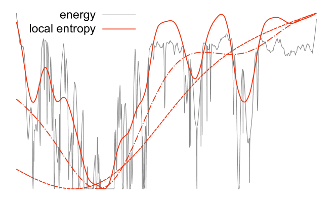
Figure 1: Energy landscape compared to local entropy landscape in an illustrative toy example. The energy landscape (gray curve) can be very rugged, with a large number of narrow local minima. Some isolated global minima can also be observed on the right. On the left, there is a region of denser minima which coalesce into a wide global optimum. The red curves show the local entropy landscape (eq. (2) with the opposite sign) computed at increasing values of the interaction parameter $\gamma$, i.e., at progressively finer scales. At low values of $\gamma$ (dashed curve), the landscape is extremely smooth and the dense region is identifiable on a coarse-grained scale. At intermediate values of $\gamma$ (dot-dashed curve) the global minimum is narrower and located in a denser region, but it does not correspond to a global energy minimum yet. At large values of $\gamma$ (solid curve) finer-grain features appear as several local minima, but the global minimum is now located inside a wide global optimum of the energy. As a consequence of this general picture, a process in which a local search algorithm driven by the local entropic landscape is run at increasing values of $\gamma$ will end up in such wide minima, even though in the limit $\gamma\to\infty$ the local entropy landscape tends to the energy landscape. Note that in a high-dimensional space the isolated global minima can be exponentially more numerous and thus dominate the equilibrium measure, but they are “filtered out” in the local entropy description.

For learning problems with discrete synapses, numerical experiments indicate that efficient algorithms also seek unfrozen solutions. In ref. baldassi_subdominant_2015 , we showed that the equilibrium description in these problems is insufficient, in the sense that it predicts that the problem is always in the completely frozen phase in which all solutions are locked huang2014origin , in spite of the fact that efficient algorithms seem to exist. This motivated us to introduce a different measure, which ignores isolated solutions and enhances the statistical weight of large, accessible regions of solutions:

$$P\left(\sigma;\beta,y,\gamma\right)=Z\left(\beta,y,\gamma\right)^{-1}e^{y\,\Phi\left(\sigma,\beta,\gamma\right)}.$$ (1)

Here $y$ is a parameter that has the formal role of an inverse temperature and $\Phi\left(\sigma,\gamma,\beta\right)$ is a “local free entropy”:

$$\Phi\left(\sigma,\beta,\gamma\right)=\log\sum_{\left\{\sigma^{\prime}\right\}}e^{-\beta E\left(\sigma^{\prime}\right)-\gamma\,d\left(\sigma,\sigma^{\prime}\right)}$$ (2)

where $d\left(\cdot,\cdot\right)$ some monotonically increasing function of the distance between configurations, defined according to the model under consideration. In the limit $\beta\to\infty$, this expression reduces (up to an additive constant) to a “local entropy”: it counts the number of minima of the energy, weighting them (via the parameter $\gamma$) by the distance from a reference configuration $\sigma$. Therefore, if $y$ is large, only the configurations $\sigma$ that are surrounded by an exponential number of local minima will have a non-negligible weight. By increasing the value of $\gamma$, it is possible to focus on narrower neighborhoods around $\sigma$, and at large values of $\gamma$ the reference $\sigma$ will also with high probability share the properties of the surrounding minima. This is illustrated in Fig. 1. These large-deviation statistics seem to capture very well the behavior of efficient algorithms on discrete neural networks, which invariably find solutions belonging to high-density regions when these regions exist, and fail otherwise. These solutions therefore could be rare (i.e., not emerge in a standard equilibrium description), and yet be accessible (i.e., there exist efficient algorithms that are able to find them), and they are inherently robust (they are immersed in regions of other “good” configurations). As discussed in baldassi_subdominant_2015 , there is a relation between the robustness of solutions in this sense and their good generalization ability: this is intuitively understood in a Bayesian framework by considering that a robust solution acts as a representative of a whole extensive region.

It is therefore natural to consider using our large-deviation statistics as a starting point to design new algorithms, in much the same way that Simulated Annealing uses equilibrium statistics. Indeed, this was shown to work well in ref. baldassi_local_2016 . The main difficulty of that approach was the need to estimate the local (free) entropy $\Phi$, which was addressed there using the Belief Propagation (BP) algorithm mezard_information_2009 .

Here we demonstrate an alternative, general and much simpler approach. The key observation is that, when $y$ is a non-negative integer, we can rewrite the partition function of the large deviation distribution eq. (1) as:

$$Z\left(\beta,y,\gamma\right) = \sum_{\left\{\sigma^{\star}\right\}}e^{y\,\Phi\left(\sigma^{\star},\beta,\gamma\right)}$$

$$= \sum_{\left\{\sigma^{\star}\right\}}\sum_{\left\{\sigma^{a}\right\}}e^{-\beta\sum_{a=1}^{y}E\left(\sigma^{a}\right)-\gamma\sum_{a=1}^{y}d\left(\sigma^{\star},\sigma^{a}\right)}$$

This partition function describes a system of $y+1$ interacting replicas of the system, one of which acts as reference while the remaining $y$ are identical, subject to the energy $E\left(\sigma^{a}\right)$ and the interaction with the reference $\sigma^{\star}$. Studying the equilibrium statistics of this system and tracing out the replicas $\sigma^{a}$ is equivalent to studying the original large deviations model. This provides us with a very simple and general scheme to direct algorithms to explore robust, accessible regions of the energy landscape: replicating the model, adding an interaction term with a reference configuration and running the algorithm over the resulting extended system.

In fact, in most cases, we can further improve on this scheme by tracing out the reference instead, which leaves us with a system of $y$ identical interacting replicas describing what we call the robust ensemble (RE):

$$Z\left(\beta,y,\gamma\right) = \sum_{\left\{\sigma^{a}\right\}}e^{-\beta\left(\sum_{a=1}^{y}E\left(\sigma^{a}\right)+A\left(\left\{\sigma^{a}\right\},\beta,\gamma\right)\right)}$$ (4)

$$A\left(\left\{\sigma^{a}\right\},\beta,\gamma\right) = -\frac{1}{\beta}\log\sum_{\sigma^{\star}}e^{-\gamma\sum_{a=1}^{y}d\left(\sigma^{\star},\sigma^{a}\right)}$$ (5)

In the following, we will demonstrate how this simple procedure can be applied to a variety of different algorithms: Simulated Annealing, Stochastic Gradient Descent, and Belief Propagation. In order to demonstrate the utility of the method, we will focus on the problem of training neural network models.

III Neural network models

Throughout this paper, we will consider for simplicity one main kind of neural network model, composed of identical threshold units arranged in a feed-forward architecture. Each unit has many input channels and one output, and is parameterized by a vector of “synaptic weights” $W$. The output of each unit is given by $\mathrm{sgn}\left(W\cdot\xi\right)$ where $\xi$ is the vector of inputs.

Since we are interested in connecting with analytical results, for the sake of simplicity all our tests have been performed using binary weights, $W_{i}^{k}\in\left\{-1,+1\right\}$, where $k$ denotes a hidden unit and $i$ an input channel. We should however mention that all the results generalize to the case of weights with multiple bits of precision baldassi2016learning . We denote by $N$ the total number of synaptic weights in the network, which for simplicity is assumed to be odd. We studied the random classification problem: given a set of $\alpha N$ random input patterns $\left\{\xi^{\mu}\right\}_{\mu=1}^{\alpha N}$, each of which has a corresponding desired output $\sigma_{D}^{\mu}\in\left\{-1,+1\right\}$, we want to find a set of parameters $W$ such that the network output equals $\sigma_{D}^{\mu}$ for all patterns $\mu$. Thus, for a single-layer network (also known as a perceptron), the condition could be written as $\sum_{\mu=1}^{\alpha N}\Theta\left(-\sigma_{D}^{\mu}\left(W\cdot\xi^{\mu}\right)\right)=0$, where $\Theta\left(x\right)=1$ if $x>0$ and $0$ otherwise. For a fully-connected two-layer neural network (also known as committee or consensus machine), the condition could be written as $\sum_{\mu=1}^{\alpha N}\Theta\left(-\sigma_{D}^{\mu}\sum_{k}\mathrm{sgn}\left(W^{k}\cdot\xi^{\mu}\right)\right)=0$ (note that this assumes that all weights in the output unit are $1$, since they are redundant in the case of binary $W$’s). A three-layer fully connected network would need to satisfy $\sum_{\mu=1}^{\alpha N}\Theta\left(-\sigma_{D}^{\mu}\sum_{l}\mathrm{sgn}\left(\sum_{k}W_{k}^{2l}\mathrm{sgn}\left(W^{1k}\cdot\xi^{\mu}\right)\right)\right)=0$, and so on. In this work, we limited our tests to one- and two-layer networks.

In all tests, we extracted all inputs and outputs in $\left\{-1,+1\right\}$ from unbiased, identical and independent distributions.

In order to use methods like Simulated Annealing and Gradient Descent, we need to associate an energy or cost to every configuration of the system $W$. One natural choice is just to count the number of errors (mis-classified patterns), but this is not a good choice for local search algorithms since it hides the information about what direction to move towards in case of error, except near the threshold. Better results can be obtained by using the following general definition instead: we define the energy $E^{\mu}\left(W\right)$ associated to each pattern $\mu$ as the minimum number of synapses that need to be switched in order to classify the pattern correctly. The total energy is then given by the sum of the energy for each pattern, $E\left(W\right)=\sum_{\mu}E^{\mu}\left(W\right)$. In the single layer case, the energy of a pattern is thus $E^{\mu}\left(W\right)=R\left(-\sigma_{D}^{\mu}\left(W\cdot\xi^{\mu}\right)\right)$, where $R\left(x\right)=\frac{1}{2}\left(x+1\right)\Theta\left(x\right)$. Despite the simple definition, the expression for the two-layer case is more involved and is provided in the Appendix A.3. For deeper networks, the definition is conceptually too naive and computationally too hard, and it should be amended to reflect the fact that more than one layer is affected by training, but this is beyond the scope of the present work.

We also need to define a distance function between replicas of the system. In all our tests, we used the squared distance $d\left(W,W^{\prime}\right)=\frac{1}{2}\sum_{i=1}^{N}\left(W_{i}-W_{i}^{\prime}\right)^{2}$, which is proportional to the Hamming distance in the binary case.

IV Replicated Simulated Annealing

We claim that there is a general strategy which can be used by a system of $y$ interacting replicas to seek dense regions of its configuration space. The simplest example of this is by sampling the configuration space with a Monte Carlo method moore2011nature which uses the objective functions given by eqs. (II) or  (4), and lowering the temperature via a Simulated Annealing (SA) procedure, until either a zero of the energy (“cost”) or a “give-up condition” is reached. For simplicity, we use the RE, in which the reference configuration is traced out (eq. (4)), and we compare our method to the case in which the interaction between the replicas is absent (i.e. $\gamma=0$, which is equivalent to running $y$ parallel independent standard Simulated Annealing algorithms on the cost function). Besides the annealing procedure, in which the inverse temperature $\beta$ is gradually increased during the simulation, we also use a “scoping” procedure, which consists in gradually increasing the interaction $\gamma$, with the effect of reducing the average distance between the replicas. Intuitively, this corresponds to exploring the energy landscape on progressively finer scales (Fig. 1).

Additionally, we find that the effect of the interaction among replicas can be almost entirely accounted for by adding a prior on the choice of the moves within an otherwise standard Metropolis scheme, while still maintaining the detailed balance condition (of course, this reduces to the standard Metropolis rule for $\gamma=0$). The elementary Monte Carlo iteration step can therefore be summarized as follows: i) we choose a replica uniformly at random; ii) we choose a candidate weight to flip for that replica according to a prior computed from the state of all the replicas; iii) we estimate the single-replica energy cost of the flip and accept it according to a standard Metropolis rule. The sampling technique (step ii above) and the parameters used for the simulations are described in the Appendix B.

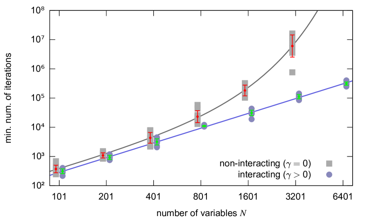
Figure 2: Replicated Simulated Annealing on the perceptron, comparison between the interacting version (i.e. which seeks regions of high solution density) and the non-interacting version (i.e. standard SA), at $\alpha=0.3$ using $y=3$ replicas. With optimized annealing/scoping parameters, the minimum number of iterations required to find a solution scales exponentially with $N$ for the standard case, and polynomially for the interacting case. $10$ samples were tested for each value of $N$ (the same samples in both cases). The bars represent averages and standard deviations (taken in logarithmic scale) while the lines represent fits. The interacting case was fitted by a function $aN^{b}$ with $a\simeq 0.13$, $b\simeq 1.7$, while the non-interacting case was fitted by a function $aN^{b}e^{cN^{d}}$ with $a\simeq 0.2$, $b\simeq 1.5$, $c\simeq 6.6\cdot 10^{-4}$ , $d\simeq 1.1$. Data is not available for the non-interacting case at $N=6401$ since we couldn’t solve any of the problems in a reasonable time (the extrapolated value according to the fit is $\sim 3\cdot 10^{9}$). The two data sets are slightly shifted relative to each other for presentation purposes. All the details are reported in the Appendix B.3.

In Fig. 2, we show the results for the perceptron; an analogous figure for the committee machine, with similar results, is shown in the Appendix, Fig. 7. The analysis of the scaling with $N$ demonstrates that the interaction is crucial to finding a solution in polynomial time: the non-interacting version scales exponentially and it rapidly becomes impossible to find solutions in reasonable times. Our tests also indicate that the difference in performance between the interacting and non-interacting cases widens greatly with increasing the number of patterns per synapse $\alpha$. As mentioned above, this scheme bears strong similarities to the Entropy-driven Monte Carlo (EdMC) algorithm that we proposed in baldassi_local_2016 , which uses the Belief Propagation algorithm (BP) to estimate the local entropy around a given configuration. The main advantage of using a replicated system is that it avoids the need to use BP, which makes the procedure much simpler and more general. On the other hand, in systems where BP is able to provide a reasonable estimate of the local entropy, it can do so directly at a given temperature, and thus avoids the need to thermalize the replicas. Therefore, the landscapes explored by the replicated SA and EdMC are in principle different, and it is possible that the latter has fewer local minima; this however does not seem to be an issue for the neural network systems considered here.

V Replicated Gradient Descent

Monte Carlo methods are computationally expensive, and may be infeasible for large systems. One simple alternative general method for finding minima of the energy is using Gradient Descent (GD) or one of its many variants. All these algorithms are generically called backpropagation algorithms in the neural networks context rumelhart1988learning . Indeed, GD—in particular Stochastic GD (SGD)—is the basis of virtually all recent successful “deep learning” techniques in Machine Learning. The two main issues with using GD are that it does not in general offer any guarantee to find a global minimum, and that convergence may be slow (in particular for some of the variables, cf. the “vanishing gradient” problem vanishing-gradient which affects deep neural network architectures). Additionally, when training a neural network for the purpose of inferring (generalizing) a rule from a set of examples, it is in general unclear how the properties of the local minima of the energy on the training set are related to the energy of the test set, i.e., to the generalization error.

GD is defined on differentiable systems, and thus it cannot be applied directly to the case of systems with discrete variables considered here. One possible work-around is to introduce a two-level scheme, consisting in using two sets of variables, a continuous one $\mathcal{W}$ and a discrete one $W$, related by a discretization procedure $W=\mathrm{discr}\left(\mathcal{W}\right)$, and in computing the gradient $\partial E\left(W\right)$ over the discrete set but adding it to the continuous set: $\mathcal{W}\leftarrow\mathcal{W}-\eta\partial E\left(W\right)$ (where $\eta$ is a gradient step, also called learning rate in the machine learning context). For the single-layer perceptron with binary synapses, using the energy definition provided above, in the case when the gradient is computed one pattern at a time (in machine learning parlance: using SGD with a minibatch size of $1$), this procedure leads to the so-called “Clipped Perceptron” algorithm (CP). This algorithm is not able to find a solution to the training problem in the case of random patterns, but simple (although non-trivial) variants of it are (SBPI and CP+R, see baldassi-et-all-pnas ; baldassi-2009 ). In particular CP+R was adapted to two-layer networks (using a a simplified version of the two-level SGD procedure described above) and was shown in baldassi_subdominant_2015 to be able to achieve near-state-of-the-art performance on the MNIST database lecun1998gradient . The two-level SGD approach was also more recently applied to multi-layer binary networks with excellent results in courbariaux2015binaryconnect ; courbariaux2016binarynet , along with an array of additional heuristic modifications of the SGD algorithm that have become standard in application-driven works (e.g., batch renormalization). In those cases, however, the back-propagation of the gradient was performed differently, either because the output of each unit was not binary courbariaux2015binaryconnect or as a work-around for the use of a different definition for the energy, which required the introduction of additional heuristic mechanisms courbariaux2016binarynet .

Almost all the above-mentioned results are purely heuristic (except in the on-line generalization setting, which is not considered in the present work). Indeed, even just using the two-level SGD is heuristic in this context. Nevertheless, here we demonstrate that, as in the case of Simulated Annealing of the previous section, replicating the system and adding a time-dependent interaction term, i.e., performing the gradient descent over the robust ensemble (RE) energy defined in eq. (5), leads to a noticeable improvement in the performance of the algorithm, and that when a solution is found it is indeed part of a dense region, as expected. We showed in baldassi_subdominant_2015 that solutions belonging to maximally dense regions have better generalization properties than other solutions; in other words, they are less prone to overfitting.

It is also important to note here that the stochastic nature of the SGD algorithm is essential in this case in providing an entropic component which counters the purely attractive interaction between replicas introduced by eq. (5), since the absolute minima of the replicated energy of eq. (4) are always obtained by collapsing all the replicas in the minima of the original energy function. Indeed, the existence of an entropic component allowed us to derive the RE definition by using the interaction strength $\gamma$ to control the distance via a Legendre transform in the first place in eq. (2); in order to use this technique with a non-stochastic minimization algorithm, the distance should be controlled explicitly instead.

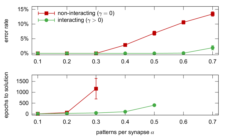
Figure 3: Replicated Stochastic Gradient descent on a fully-connected committee machine with $N=1605$ synapses and $K=5$ units in the second layer, comparison between the non-interacting (i.e. standard SGD) and interacting versions, using $y=7$ replicas and a minibatch size of $80$ patterns. Each point shows averages and standard deviations on $10$ samples with optimal choice of the parameters, as a function of the training set size. Top: minimum training error rate achieved after $10^{4}$ epochs. Bottom: number of epochs required to find a solution. Only the cases with $100\%$ success rate are shown (note that the interacting case at $\alpha=0.6$ has $50\%$ success rate but an error rate of just $0.07\%$).

In Fig. 3 we show the results for a fully connected committee machine, demonstrating that the introduction of the interaction term greatly improves the capacity of the network (from $0.3$ to almost $0.6$ patterns per synapse), finds configurations with a lower error rate even when it fails to solve the problem, and generally requires fewer presentations of the dataset (epochs). The graphs show the results for $y=7$ replicas in which the gradient is computed for every $80$ patterns (the so-called minibatch size); we observed the same general trend for all cases, even with minibatch sizes of $1$ (in the Appendix, Fig. 8, we show the results for $y=3$ and minibatch size $10$). We also observed the same effect in the perceptron, although with less extensive tests, where this algorithm has a capacity of at least $0.7$. All technical details are provided in Appendix C. These results are in perfect agreement with the analysis of the next section, on Belief Propagation, which suggests that this replicated SGD algorithm has near-optimal capacity.

It is interesting to note that a very similar approach—a replicated system in which each replica is attracted towards a reference configuration, called Elastic Averaged SGD (EASGD)—was proposed in NIPS2015_5761 (see also zhang2016distributed ) using deep convolutional networks with continuous variables, as a heuristic way to exploit parallel computing environments under communication constraints. Although it is difficult in that case to fully disentangle the effect of replicating the system from the other heuristics (in particular the use of “momentum” in the GD update), their results clearly demonstrate a benefit of introducing the replicas in terms of training error, test error and convergence time. It seems therefore plausible that, despite the great difference in complexity between their network and the simple models studied in this paper, the general underlying reason for the effectiveness of the method is the same, i.e., the existence of accessible robust low-energy states in the space of configurations work-in-progress .

VI Replicated Belief Propagation

Belief Propagation (BP), also known as Sum-Product, is an iterative message-passing method that can be used to describe a probability distribution over an instance described by a factor graph in the correlation decay approximation mackay2003information ; yedidia2005constructing . The accuracy of the approximation relies on the assumption that, when removing an interaction from the network, the nodes involved in that interaction become effectively independent, an assumption linked to so-called Replica Symmetry (RS) in statistical physics.

Algorithmically, the method can be briefly summarized as follows. The goal is to solve a system of equations involving quantities called messages. These messages represent single-variable cavity marginal probabilities, where the term “cavity” refers to the fact that these probabilities neglect the existence of a node in the graph. For each edge of the graph there are two messages going in opposite directions. Each equation in the system gives the expression of one of the messages as a function of its neighboring messages. The expressions for these functions are derived from the form of the interactions between the variables of the graph. The resulting system of equations is then solved iteratively, by initializing the messages in some arbitrary configuration and updating them according to the equations until a fixed point is eventually reached. If convergence is achieved, the messages can be used to compute various quantities of interest; among those, the most relevant in our case are the single-site marginals and the thermodynamic quantities such as the entropy and the free energy of the system. From single-site marginals, it is also possible to extract a configuration by simply taking the $\mathrm{argmax}$ of each marginal.

In the case of our learning problem, the variables are the synaptic weights, and each pattern represents a constraint (i.e., an “interaction”) between all variables, and the form of these interactions is such that BP messages updates can be computed efficiently. Also note that, since our variables are binary, each of the messages and marginals can be described with a single quantity: we generally use the magnetization, i.e., the difference between the probability associated to the states $+1$ and $-1$. We thus generally speak of the messages as “cavity magnetizations” and the marginals as “total magnetizations”. The factor graph, the BP equations and the procedure to perform the updates efficiently are described in detail in the Appendix section D.1, closely following the work of braunstein-zecchina . Here, we give a short summary. We use the notation $m_{j\to\mu}^{t}$ for the message going from the node representing the weight variable $j$ to the node representing pattern $\mu$ at iteration step $t$, and $m_{\mu\to j}^{t}$ for the message going in the opposite direction, related by the BP equation:

$$m_{j\to\mu}^{t} = \tanh\sum_{\nu\in\partial j\setminus\mu}\tanh^{-1}m_{\nu\to j}^{t}$$ (6)

where $\partial j$ indicates the set of all factor nodes connected to $j$. The expressions for the total magnetizations $m_{j}^{t}$ are identical except that the summation index runs over the whole set $\partial j$. A configuration of the weights is obtained from the total magnetizations simply as $W_{j}=\mathrm{sgn}\left(m_{j}\right)$. The expression for $m_{\nu\to j}^{t+1}$ as a function of $\left\{m_{i\to\nu}^{t}\right\}_{i=1}^{N}$ is more involved and it’s reported in the Appendix section D.1.

As mentioned above, BP is an inference algorithm: when it converges, it describes a probability distribution. One particularly effective scheme to turn BP into a solver is the addition of a “reinforcement” term braunstein-zecchina : a time-dependent local field is introduced for each variable, proportional to its own marginal probability as computed in the previous iteration step, and is gradually increased until the whole system is completely biased toward one configuration. This admittedly heuristic scheme is quite general, leads to very good results in a variety of different problems, and can even be used in cases in which unmodified BP would not converge or would provide a very poor approximation (see e.g. bailly2011finding ). In the case of the single layer binary network such as those considered in this paper, it can reach a capacity of $\alpha\simeq 0.75$ patterns per synapse braunstein-zecchina , which is consistent with the value at which the structure of solution-dense regions breaks baldassi_subdominant_2015 .

The reason for the effectiveness of reinforced BP has not been clear. Intuitively, the process progressively focuses on smaller and smaller regions of the configuration space, with these regions determined from the current estimate of the distribution by looking in the “most promising” direction. This process has thus some qualitative similarities with the search for dense regions described in the previous sections. This analogy can be made precise by writing the BP equations for the system described by eq. (II). There are in this case two equivalent approaches: the first is to use the local entropy as the energy function, using a second-level BP to estimate the local entropy itself. This approach is very similar to the so called 1-step replica-symmetry-breaking (1RSB) cavity equations (see  mezard_information_2009 for a general introduction). The second approach is to replicate the system, considering $N$ vector variables $\left\{W_{j}^{a}\right\}_{a=1}^{y}$ of length $y$, and assuming an internal symmetry for each variable, i.e. that all marginals are invariant under permutation of the replica indices, similarly to what is done in kabashima2005 : $P_{j}\left(\left\{W_{j}^{a}\right\}_{a=1}^{y}\right)=P_{j}\left(\sum_{a=1}^{y}W_{j}^{a}\right)$. The result in the two cases is the same (this will be shown in a technical work, in preparation, where the connection between the large deviations measure and the 1RSB equilibrium description is also made explicit). Since BP assumes replica symmetry, the resulting message passing algorithm reproduces quite accurately the analytical results at the RS level. As explained in baldassi_subdominant_2015 , these results can however become wrong, in particular for high values of $\alpha$, $\gamma$ and $y$, due to the onset of correlations (the so called replica-symmetry-breaking – RSB – effect mezard_information_2009 ). More specifically, in this model the RS solution assumes that there is a single dense region comprising the robust ensemble (RE), while the occurrence of RSB implies that there are several maximally dense regions. As a consequence this algorithm is not a very good candidate as a solver. A more correct description—which could then lead to a more controlled solver—would thus require a third level of BP equations, or equivalently an assumption of symmetry-breaking in the structure of the marginals $P_{j}\left(\left\{W_{j}^{a}\right\}_{a=1}^{y}\right)$.

Figure 4: A. Portion of a BP factor graph for a replicated variable $W_{j}$ with $y=3$ replicas and a reference configuration $W_{j}^{\star}$. The dashed lines represent edges with the rest of the factor graph. The squares represent the interactions $\gamma W_{j}^{\star}W_{j}^{a}$. All BP messages (arrows) are assumed to be the same in corresponding edges. B. Transformed graph which represents the same graph as in A but exploits the symmetry to reduce the number of nodes, keeping only one representative per replica. The hexagon represents a pseudo-self-interaction, i.e. it expresses the fact that $m_{\star\to j}$ depends on $m_{j\to\star}$ and is parametrized by $\gamma$ and $y$.

Fortunately, it turns out that that there is a different way of applying BP to the replicated system, leading to an efficient solver which is both very similar to the reinforced BP algorithm and reasonably well described by the theoretical results. Instead of considering the joint distribution over all replicated variables at a certain site $j$, we simply replicate the original factor graph $y$ times; then, for each site $j$, we add an extra variable $W_{j}^{\star}$, and $y$ interactions, between each variable $W_{j}^{a}$ and $W_{j}^{\star}$. Finally, since the problem is symmetric, we assume that each replica of the system behaves in exactly the same way, and therefore that the same messages are exchanged along the edges of the graph regardless of the replica index. This assumption neglects some of the correlations between the replicated variables, but allows us to work only with a single system, which is identical to the original one except that each variable now also exchanges messages with $y-1$ identical copies of itself through an auxiliary variable (which we can just trace away at this point, as in eq. (4)). The procedure is shown graphically in Fig. 4. At each iteration step $t$, each variable receives an extra message of the form:

$$m_{\star\to j}^{t+1}=\tanh\left(\left(y-1\right)\tanh^{-1}\left(m_{j\to\star}^{t}\tanh\gamma\right)\right)\tanh\gamma$$ (7)

where $m_{j\to\star}^{t}$ is the cavity magnetization resulting from the rest of the factor graph at time $t$, and $\gamma$ is the interaction strength. This message simply enters as an additional term in the sum in the right-hand side of eq. (6). Note that, even though we started from a system of $y$ replicas, after the transformation we are no longer constrained to keep $y$ in the integer domain. The reinforced BP braunstein-zecchina , in contrast, would have a term of the form:

$$m_{\star\to j}^{t+1}=\tanh\left(\rho\tanh^{-1}m_{j}^{t}\right)$$ (8)

The latter equation uses a single parameter $0\leq\rho\leq 1$ instead of two, and is expressed in terms of the total magnetization $m_{j}^{t}$ instead of the cavity magnetization $m_{j\to\star}^{t}$. Despite these differences, these two terms induce exactly the same BP fixed points if we set $\gamma=\infty$ and $y=\left(1-\rho\right)^{-1}$ (see the Appendix section D.2). This result is somewhat incidental, since in the context of our analysis the limit $\gamma\to\infty$ should be reached gradually, otherwise the results should become trivial (see figure 1), and the reason why this does not happen when setting $\gamma=\infty$ in eq. (7) is only related to the approximations introduced by the simplified scheme of figure (4). As it turns out, however, choosing slightly different mappings with both $\gamma$ and $y$ diverging gradually (e.g. $\gamma=\tanh^{-1}\sqrt{\rho}$ and $y=\frac{2-\rho}{1-\rho}$ with $\rho$ increasing from $0$ to $1$) can lead to update rules with the same qualitative behavior and very similar quantitative effects, such that the performances of the resulting algorithms are hardly distinguishable, and such that the aforementioned approximations do not thwart the consistency with the theoretical analysis. This is shown and discussed Appendix D.2. Using a protocol in which $\gamma$ is increased gradually, rather than being set directly at $\infty$, also allows the algorithm to reach a fixed point of the BP iterative scheme before proceeding to the following step, which offers more control in terms of the comparison with analytical results, as discussed in the next paragraph. In this sense, we therefore have derived a qualitative explanation of the effectiveness of reinforced BP within a more general scheme for the search of accessible dense states. We call this algorithm Focusing BP (fBP).

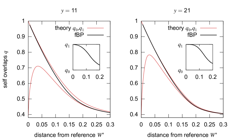
Figure 5: Focusing BP (fBP) spontaneously breaks replica symmetry: the overlap order parameter $q$ (black thick curves) gradually transitions from the inter-cluster overlap $q_{0}$ and the intra-cluster overlap $q_{1}$ of the replica theory (red thin curves, $q_{0}<q_{1}$) as the distance to the reference $W^{\star}$ goes to $0$ (i.e. as $\gamma\to\infty$). The insets provide an alternative visualization of this phenomenon, plotting $\left(q-q_{0}\right)/\left(q_{1}-q_{0}\right)$ against the distance. These results were obtained on a perceptron with $N=1001$ at $\alpha=0.6$, averaging over $50$ samples. The two panels shows that the transition occurs at larger distances (i.e. at smaller $\gamma$) at larger $y$.

Apart from the possibility of using fBP as a solver, by gradually increasing $\gamma$ and $y$ until a solution is found, it is also interesting to compare its results at fixed values of $y$ and $\gamma$ with the analytical predictions for the perceptron case which were derived in baldassi_subdominant_2015 ; baldassi_local_2016 , since at the fixed point we can use the fBP messages to compute such values as the local entropy, the distance from the reference configuration, and the average overlap between replicas (defined as $q=\frac{1}{N}\sum_{j}\left\langle W_{j}^{a}\right\rangle\left\langle W_{j}^{b}\right\rangle$ for any $a$ and $b$, where $\left\langle\cdot\right\rangle$ denotes the thermal averaging). The expressions for these quantities are provided in Appendix D.1. The results indicate that fBP is better than the alternatives described above in overcoming the issues arising from RSB effects. The 1RSB scheme describes a non-ergodic situation which arises from the break-up of the space of configurations into a collection of several separate equivalent ergodic clusters, each representing a possible state of the system. These states are characterized by the typical overlap inside the same state (the intra-cluster overlap $q_{1}$) and the typical overlap between configurations from any two different states (the inter-cluster overlap $q_{0}$). Fig. 5 shows that the average overlap $q$ between replicas computed by the fBP algorithm transitions from $q_{0}$ to $q_{1}$ when $\gamma$ is increased (and the distance with the reference is decreased as a result). This suggests that the algorithm has spontaneously chosen one of the possible states of high local entropy in the RE, achieving an effect akin to the spontaneous symmetry breaking of the 1RSB description. Within the state, replica symmetry holds, so that the algorithm is able to eventually find a solution to the problem. Furthermore, the resulting estimate of the local entropy is in very good agreement with the 1RSB predictions up to at least $\alpha=0.6$ (see the Appendix, figure 11).

Therefore, although this algorithm is not fully understood from the theoretical point of view, it offers a valuable insight into the reason for the effectiveness of adding a reinforcement term to the BP equations. It is interesting in this context to observe that the existence of a link between the reinforcement term and the robust ensemble seems consistent with some recent results on random bicoloring constraint satisfaction problems braunstein_large_2016 , which showed that reinforced BP finds solutions with shorter “whitening times” with respect to other solvers: this could be interpreted as meaning they belong to a region of higher solution density, or are more central in the cluster they belong to. Furthermore, our algorithm can be used to estimate the point up to which accessible dense states exist, even in cases, like multi-layer networks, where analytical calculations are prohibitively complex.

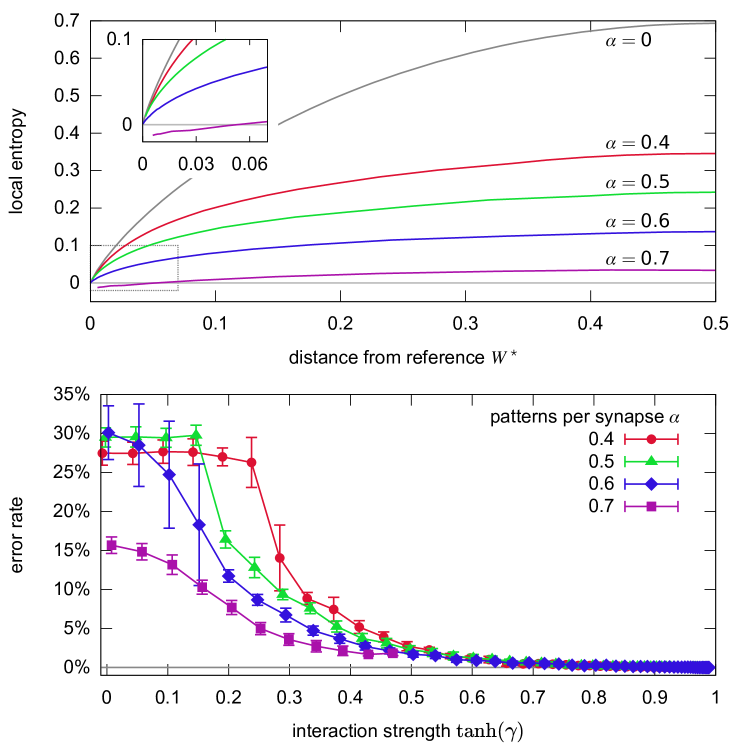
Figure 6: Results of fBP on a committee machine with $N=1605$, $K=5$, $y=7$, increasing $\gamma$ from $0$ to $2.5$, averages on $10$ samples. Top: local entropy versus distance to the reference $W^{\star}$ for various $\alpha$ (error bars not shown for clarity). The topmost gray curve ($\alpha=0$) is an upper bound, representing the case where all configurations within some distance are solutions. Inset: enlargement of the region near the origin indicated by the rectangle in the main plot. This shows that dense states exist up to almost $\alpha=0.6$: at this value of $\alpha$, dense states are only found for a subset of the samples (in which case a solution is also found). Negative local entropies (curve at $\alpha=0.7$) are unphysical, and fBP fails shortly after finding such values. Bottom: error rates as a function of $\tanh\left(\gamma\right)$. For $\alpha\leq 0.6$, all curves eventually get to $0$. However, only $7$ out of $10$ samples reached a sufficiently high $\gamma$ at $\alpha=0.6$, while in $3$ cases the fBP equations failed. The curve for $\alpha=0.7$ is interrupted because fBP failed for all samples, in each case shortly after reaching a negative local entropy. The plateaus at $\alpha=0.4$ and $\alpha=0.5$ are regions where the solution to the equations are symmetric with respect to the permutation of the hidden units: fBP spontaneously breaks that symmetry as well.

Fig. 6 shows the result of experiments performed on a committee machine with the same architecture and same $y$ of Fig. 3. The implementation closely follows braunstein-zecchina with the addition of the self-interaction eq. (7), except that great care is required to correctly estimate the local entropy at large $\gamma$, due to numerical issues (see Appendix D.1). The figure shows that fBP finds that dense states (where the local entropy curves approach the upper bound at small distances) exist up to nearly $\alpha=0.6$ patterns per synapse, and that when it finds those dense states it is correspondingly able to find a solution, in perfect agreement with the results of the replicated gradient descent algorithm.

Finally, we also performed some exploratory tests applying fBP on the random $K$-satisfiability problem, and we found clear indications that the performance of this algorithm is similar to that of Survey-Propagation-based algorithms mezard2002analytic ; marino2015backtrackingSP , although a more detailed analysis is required to draw a more precise comparison.. The results are reported in Appendix D.4.

VII Discussion

In this paper, we have presented a general scheme that can be used to bias the search for low-energy configurations, enhancing the statistical weight of large, accessible states. Although the underlying theoretical description is based on a non-trivial large deviation measure, its concrete implementation is very simple—replicate the system and introduce an interaction between the replicas—and versatile, in that it can be generally applied to a number of different optimization algorithms or stochastic processes. We demonstrated this by applying the method to Simulated Annealing, Gradient Descent and Belief Propagation, but it is clear that the list of possible applications may be much longer. The intuitive interpretation of the method is also quite straightforward: a set of coupled systems is less likely to get trapped in narrow minima, and will instead be attracted to wide regions of good (and mostly equivalent) configurations, thus naturally implementing a kind of robustness to details of the configurations.

The utility of this kind of search depends on the details of the problem under study. Here we have mainly focused on the problem of training neural networks, for a number of reasons. The first is that, at least in the case of single-layer networks with discrete synapses, we had analytical and numerical evidence that dense, accessible states exist and are crucial for learning and improving the generalization performance, and we could compare our findings with analytical results. The second is that the general problem of training neural networks has been addressed in recent years via a sort of collective search in the space of heuristics, fueled by impressive results in practical applications and mainly guided by intuition; heuristics are evaluated based on their effectiveness in finding accessible states with good generalization properties. It seems reasonable to describe these accessible states as regions of high local entropy, i.e., wide, very robust energy minima: the center of such a region can act as a Bayesian estimator for the whole extensive neighborhood. Here we showed a simple way to exploit the existence of such states efficiently, whatever the optimization algorithm used. This not only sheds light on previously known algorithms, but also suggests improvements or even entirely new algorithms. Further work is required to determine whether the same type of phenomenon that we observed here in simple models actually generalizes to the deep and complex networks currently used in machine learning applications (the performance boost obtained by the EASGD algorithm of NIPS2015_5761 being a first indication in this direction), and to investigate further ways to improve the performance of learning algorithms, or to overcome constraints (such as being limited to very low-precision computations).

It is also natural to consider other classes of problems in which this analysis may be relevant. One application would be solving other constraint satisfaction problems. For example, in baldassi_local_2016 we demonstrated that the EdMC algorithm can be successfully applied to the random $K$-satisfiability problem, even though we had to resort to a rough estimate of the local entropy due to replica symmetry breaking effects. We have shown here that the fBP algorithm presented above is also effective and efficient on the same problem. It is also interesting to note here that large-deviation analyses—although different from the one of the present paper—of a similar problem, the random bicoloring constraint satisfaction problem,dall2008entropy ; braunstein_large_2016 have shown that atypical “unfrozen” solutions exist (and can be found with the reinforced BP algorithm) well beyond the point in the phase diagram where the overwhelming majority of solutions have become “frozen”. Finally, an intriguing problem is the development of a general scheme for a class of out-of-equilibrium processes attracted to accessible states: even when describing a system which is unable to reach equilibrium in the usual thermodynamic sense or is driven by some stochastic perturbation, it is still likely that its stationary state can be characterized by a large local entropy.

Appendix A Model and notation

This Appendix text contains all the technical details of the algorithms described in the main text, the techniques and the parameters we used to obtain the results we reported. We also report some additional results and report other minor technical considerations.

Preliminarily, we set a notation used throughout the rest of this document which is slightly different from the one of the main text, but more suitable for this technical description.

A.1 The network model

As described in the main text, we consider an ensemble of $y$ neural networks with $K$ units and binary variables $W_{i}^{ka}\in\left\{-1,1\right\}$ where $k\in\left\{1,\ldots,K\right\}$ is the unit index, $i\in\left\{1,\ldots,\nicefrac{{N}}{{K}}\right\}$ is the synaptic index and $a\in\left\{1,\ldots,y\right\}$ is the replica index. Each network has thus $N$ synapses, where $N$ is divisible by $K$. For simplicity, we assume both $K$ and $\nicefrac{{N}}{{K}}$ to be odd. The output of each unit is defined by a function $\tau\left(\xi;W\right)=\operatorname*{sign}\left(\sum_{i=1}^{N/K}W_{i}\xi_{i}\right)$. The output of the network is defined by a function $\zeta\left(\left\{\xi^{k}\right\}_{k};\left\{W^{k}\right\}_{k}\right)=\operatorname*{sign}\left(\sum_{k=1}^{K}\tau\left(\xi^{k};W^{k}\right)\right)$ where $\xi^{k}$ represents the input to the $k$-th unit. In the case $K=1$, this is equivalent to a single-layer network (also known as perceptron). In the case where all $\xi^{k}$ are identical for each $k$, this is equivalent to a fully-connected two-layer network (also known as committee machine or consensus machine). If the $\xi^{k}$ are different for different values of $k$, this is a tree-like committee machine. Note that, due to the binary constraint on the model, adding weights to the second layer is redundant, since for all negative weights in the second layer we could always flip both its weight and all the weights of the unit connected to it. Therefore, without loss of generality, we just set the weights of the second layer to $1$, resulting in the above definition of the output function $\zeta$.

The scalar product between two replicas $a$ and $b$ is defined as $W^{a}\cdot W^{b}=\sum_{k=1}^{K}\sum_{i=1}^{N/K}W_{i}^{ka}W_{i}^{kb}$. For brevity of notation, in cases where the unit index does not play a role, we will often just use a single index $j\in\left\{1,\ldots,N\right\}$, e.g. $W^{a}\cdot W^{b}=\sum_{j=1}^{N}W_{j}^{a}W_{j}^{b}$.

A.2 Patterns

The networks are trained on random input/output associations, i.e. patterns, $\left(\xi^{\mu},\sigma_{D}^{\mu}\right)$ where $\mu\in\left\{1,\ldots,\alpha N\right\}$ is the pattern index. The parameter $\alpha>0$ determines the load of the network, so that the number of patterns is proportional to the number of synapses. The inputs are binary vectors of $N$ elements with entries $\xi_{i}^{k\mu}\in\left\{-1,+1\right\}$, and the desired outputs are also binary, $\sigma_{D}^{\mu}\in\left\{-1,+1\right\}$. Both the inputs and the outputs are extracted at random and are independent and identically distributed (i.i.d.), except in the case of the fully-connected committee machine where $\xi_{i}^{k\mu}=\xi_{i}^{k^{\prime}\mu}$ for all $k,k^{\prime}$ and therefore we only extract the values for $k=1$.

We also actually exploit a symmetry in the problem and set all desired outputs to $1$, since for each pattern its opposite must have an opposite output, i.e. we can always transform an input output pair $\left(\xi^{\mu},\sigma_{D}^{\mu}\right)$ into $\left(\xi^{\mu\prime},1\right)$, where the new pattern $\xi^{\mu\prime}=\sigma_{D}^{\mu}\xi^{\mu}$ has the same probability as $\xi^{\mu}$.

A.3 Energy definition

The energy, or cost, for each pattern is defined as the minimum number of weights which need to be switched in order to correctly classify the pattern, i.e. in order to satisfy the relation $\zeta\left(\left\{\xi^{k\mu}\right\}_{k},\left\{W^{k}\right\}_{k}\right)=1$. The total energy is the sum of the energies for all patterns, $E\left(W\right)=\sum_{\mu=1}^{\alpha N}E^{\mu}\left(W\right)$.

If the current configuration of the weights $W$ satisfies the pattern, the corresponding energy is obviously $0$. Therefore, if the training problem is satisfiable, the ground states with this energy definition are the same as for the easier energy function given in terms of the number of errors.

If the current configuration violates the pattern, the energy can be computed as follows: we need to compute the minimum number $c^{\mu}$ of units of the first level which need to change their outputs, choose the $c^{\mu}$ units which are easiest to fix, and for each of them compute the minimum number of weights which need to be changed. In formulas:

$$E^{\mu}\left(W\right)=\Theta\left(-\Delta_{\mathrm{out}}^{\mu}\right)\sum_{k=1}^{c^{\mu}}s_{k}^{\mu}$$ (9)

where:

$$\Delta_{k}^{\mu} = \xi^{k\mu}\cdot W^{k}$$ (10)

$$\Delta_{\mathrm{out}}^{\mu} = \sum_{k}\operatorname*{sign}\left(\Delta_{k}^{\mu}\right)$$ (11)

$$s^{\mu} = \operatorname*{sort}\left(\left\{-\frac{1}{2}\left(\Delta_{k}^{\mu}-1\right),\;\forall k:\Delta_{k}^{\mu}<0\right\}\right)$$ (12)

$$c^{\mu} = \frac{1}{2}\left(-\Delta_{\mathrm{out}}^{\mu}+1\right)$$ (13)

where the $\operatorname*{sort}\left(\cdot\right)$ function returns its argument sorted in ascending order. The above auxiliary quantities all depend on $W$, but we omitted the dependency for clarity of notation.

In the single-layer case $K=1$ the expression simplifies considerably, since $\Delta_{\mathrm{out}}^{\mu}=\xi^{\mu}\cdot W$ and reduces to $E^{\mu}\left(W\right)=\Theta\left(-\Delta_{\mathrm{out}}^{\mu}\right)\frac{1}{2}\left(-\Delta_{\mathrm{out}}^{\mu}+1\right)$ .

Appendix B Replicated Simulated Annealing

We run Simulated Annealing (plus “scoping”) on a system of interacting replicas. For simplicity, we trace away the reference configuration which mediates the interaction. Thus, at any given step, we want to sample from a probability distribution

$$P\left(\left\{W^{a}\right\}\right) \propto \sum_{W}\exp\left(-\beta\sum_{a=1}^{y}E\left(W^{a}\right)+\gamma\sum_{a=1}^{y}\sum_{j=1}^{N}W_{j}^{a}W_{j}\right)$$ (14)

$$\propto \exp\left(-\beta\sum_{a=1}^{y}E\left(W^{a}\right)+\sum_{j}\log\left(2\cosh\left(\gamma\sum_{a=1}^{y}W_{j}^{a}\right)\right)\right)$$

The reference configuration is traced out in this representation, but we can obtain its most probable value by just computing $\tilde{W}_{j}=\mathrm{sign}\sum_{a=1}^{y}W_{j}^{a}$. It is often the case that, when the parameters are chosen appropriately, $E\left(\tilde{W}\right)\leq\left\langle E\left(W^{a}\right)\right\rangle_{a}$, i.e. that the energy of the center is lower than that of the group of replicas. In fact, we found this to be a good rule-of-thumb criterion to evaluate the choice of the parameters in the early stages of the algorithmic process.

The most straightforward way to perform the sampling (at fixed $\beta$ and $\gamma$) is by using the Metropolis rule; the proposed move is to flip a random synaptic weight from a random replica. Of course the variation of the energy associated to the candidate move now includes the interaction term, parametrized by $\gamma$, which introduces a bias that favors movements in the direction of the center of mass of the replicas.

We also developed an alternative rule for choosing the moves in a biased way which implicitly accounts for the interaction term while still obeying the detailed balance condition. This alternative rule is generally valid in the presence of an external field and is detailed at the end of this section. Its advantage consists in reducing the rejection rate, but since the move proposal itself becomes more time consuming it is best suited to systems in which computing the energy cost of a move is expensive, so its usefulness depends on the details of the model.

B.1 Computing the energy shifts efficiently

Here we show how to compute efficiently the quantity $E\left(W^{\prime}\right)-E\left(W\right)$ when $W^{\prime}$ and $W$ only differ in the value of one synaptic weight $j$ and the energy is defined as in eq. (9). To this end, we define some auxiliary quantities in addition to the ones required for the energy computation, eqs. (10)-(13) (note that we omit the replica index $a$ here since this needs to be done for each replica independently):

$$P^{+} = \left\{\mu:\Delta_{\mathrm{out}}^{\mu}=1\right\}$$ (15)

$$P^{-} = \left\{\mu:\Delta_{\mathrm{out}}^{\mu}<0\right\}$$ (16)

$$\chi^{\mu} = \begin{cases}1&\textrm{if}\>s^{\mu}<0\wedge c^{\mu}<K\wedge s_{c^{\mu}}^{\mu}=s_{c^{\mu}+1}^{\mu}\\ 0&\mathrm{otherwise}\end{cases}$$ (17)

These quantities must be recomputed each time a move is accepted, along with (10)-(13). Note however that in later stages of the annealing process most moves are rejected, and the energy shifts can be computed very efficiently as we shall see below.

Preliminarily, we note that any single-flip move only affects the energy contribution from patterns in $P^{+}\cup P^{-}$.

The contribution to the energy shift $\Delta E^{\mu}$ for a proposed move $W_{i}^{k}\rightarrow-W_{i}^{k}$ is most easily written in pseudo-code:

1if $\mu\in P^{+}$ then

2       if $\xi_{i}^{\mu}\neq W_{i}^{k\mu}$ then return 0

3      

4       if $\operatorname*{sign}\left(\Delta_{k}^{\mu}\right)\neq 1$ then return 0

5      

6       return 1

7      

8 else if $\mu\in P^{-}$ then

9       if $\Delta_{k}^{\mu}>1$ then return 0

10      

11       $d:=-\xi_{i}^{\mu}W_{i}^{k\mu}$

12       if $\Delta_{k}^{\mu}>0\wedge d=1$ then return 0

13      

14       if $\Delta_{k}^{\mu}=1$ then return 1

15      

16       $v:=-(\Delta_{k}^{\mu}+1)/2+1$

17       if $v>s^{\mu}_{c^{\mu}}$ then return 0

18      

19       if $v<s^{\mu}_{c^{\mu}}$ then return -d

20      

21       if $d=1$ then return -1

22      

23       if $\chi^{\mu}=1$ then return 0

24      

25       return 1

26      

27 else

28       return 0

29      

30 end if

Algorithm 1 Energy shift function $\Delta E^{\mu}\left(\mu,\,k,\,i,\,W_{i}^{k\mu}\right)$

Indeed, this function is greatly simplified in the single-layer case $K=1$.

B.2 Efficient Monte Carlo sampling

Here we describe a Monte Carlo sampling method which is a modification of the Metropolis rule when the system uses $N$ binary variables $W_{j}$ and the Hamiltonian function can be written as:

$$H\left(W\right)=E\left(W\right)-\frac{1}{\beta}\sum_{j=1}^{N}k_{j}W_{j}$$ (18)

where the external fields $k_{j}$ can only assume a finite (and much smaller than $N$) set of values. The factor $\beta^{-1}$ is introduced merely for convenience. Comparing this to eq. (14), we see that, having chosen a replica index $a$ uniformly at random, we can identify

$$k_{j}=\frac{1}{2}\left(\log\left(\frac{\cosh\left(\gamma+\gamma\sum_{b\neq a}W_{j}^{b}\right)}{\cosh\left(-\gamma+\gamma\sum_{b\neq a}W_{j}^{b}\right)}\right)\right)$$ (19)

.

Given a transition probability to go from state $W$ to state $W^{\prime}$, $P\left(W\to W^{\prime}\right)$, the detailed balance equation reads:

$$P\left(W\right)P\left(W\to W^{\prime}\right)=P\left(W^{\prime}\right)P\left(W^{\prime}\to W\right)$$ (20)

Let us split the transition explicitly in two steps: choosing the index $j$ and accepting the move. The standard Metropolis rule is: pick an index $j\in\left\{1,\dots,N\right\}$ uniformly at random, propose the flip of $W_{j}$, accept it with probability $\min\left(1,e^{-\beta\Delta E_{W\to W^{\prime}}-2k_{j}W_{j}}\right)$, where $\Delta E_{W\to W^{\prime}}=E\left(W^{\prime}\right)-E\left(W\right)$. We want to reduce the rejection rate and incorporate the effect of the field in the proposal instead. We write:

$$P\left(W\to W^{\prime}\right)=C\left(W\to W^{\prime}\right)A\left(W\to W^{\prime}\right)$$ (21)

where $C$ is the choice of the index, and $A$ is the acceptance of the move. Usually $C$ is uniform and we ignore it, but here instead we try to use it to absorb the external field term in the probability distribution. From detailed balance we have:

$$\frac{A\left(W\to W^{\prime}\right)}{A\left(W^{\prime}\to W\right)} = \frac{p\left(W^{\prime}\right)}{p\left(W\right)}\frac{C\left(W^{\prime}\to W\right)}{C\left(W\to W^{\prime}\right)}$$ (22)

$$= e^{-\beta\Delta E_{W\to W^{\prime}}-2k_{j}W_{j}}\frac{C\left(W^{\prime}\to W\right)}{C\left(W\to W^{\prime}\right)}$$

so if we could satisfy:

$$e^{-2k_{j}W_{j}}\frac{C\left(W^{\prime}\to W\right)}{C\left(W\to W^{\prime}\right)}=1$$ (23)

then the acceptance $A$ would simplify to the usual Metropolis rule, involving only the energy shift $\Delta E$. This will turn out to be impossible, yet easily fixable, so we still first derive the condition implied by eq. (23). The key observation is that there is a finite number of classes of indices in $W$, based on the limited number of values that $W_{j}k_{j}$ can take (in the case of eq. (19) there are $y$ possible values). Let us call $K_{c}$ the possible classes, such that $W_{j}\in K_{c}\Leftrightarrow W_{j}k_{j}=c$, and let us call $n_{c}=\left|K_{c}\right|$ their sizes, with the normalization condition that $\sum_{c}n_{c}=N$. Within a class, we must choose the move $j$ uniformly.

Then $C\left(W\to W^{\prime}\right)$ is determined by the probability of picking a class, which in principle could be a function of all the values of the $n_{c}$: $P_{c}\left(\left\{n_{c^{\prime}}\right\}_{c^{\prime}}\right)$. Suppose now that we have picked an index in a class $K_{c}$. The transition to $W^{\prime}$ would bring it into class $K_{-c}$, and the new class sizes would be

$$n_{c^{\prime}}^{\prime}=\begin{cases}n_{c^{\prime}}+1&\mathrm{if}\>c^{\prime}=-c\\ n_{c^{\prime}}-1&\mathrm{if}\>c^{\prime}=c\\ n_{c^{\prime}}&\mathrm{otherwise}\end{cases}$$

therefore:

$$\frac{C\left(W^{\prime}\to W\right)}{C\left(W\to W^{\prime}\right)}=\frac{n_{c}}{P_{c}\left(\left\{n_{c^{\prime}}\right\}_{c^{\prime}}\right)}\frac{P_{-c}\left(\left\{n_{c^{\prime}}^{\prime}\right\}_{c^{\prime}}\right)}{n_{-c}+1}$$ (24)

Since the only values of $n_{c^{\prime}}$ directly involved in this expression are $n_{c}$ and $n_{-c}$, it seems reasonable to restrict the dependence of $P_{c}$ and $P_{-c}$ only on those values. Let us also call $q_{c}=n_{c}+n_{-c}$, which is unaffected by the transition. Therefore we can just write:

$$\frac{C\left(W^{\prime}\to W\right)}{C\left(W\to W^{\prime}\right)}=\frac{n_{c}}{q_{c}-n_{c}+1}\frac{P_{-c}\left(q_{c}-n_{c}+1,q_{c}\right)}{P_{c}\left(n_{c},q_{c}\right)}$$ (25)

Furthermore, we can assume – purely for simplicity – that:

$$P_{c}\left(n_{c},q_{c}\right)+P_{-c}\left(q_{c}-n_{c},q_{c}\right)=\frac{q_{c}}{N}$$ (26)

which allows us to restrict ourselves in the following to the case $c>0$, and which implies that the choice of the index will proceed like this: we divide the indices in super-classes $D_{c}=K_{c}\cup K_{-c}$ of size $q_{c}$ and we choose one of those according to their size; then we choose either the class $K_{c}$ or $K_{-c}$ according to $P_{c}\left(n_{c},q_{c}\right)$; finally, we choose an index inside the class uniformly at random. Considering this process, what we actually need to determine is the conditional probability of choosing $K_{c}$ once we know we have chosen the super-class $D_{c}$:

$$\hat{P}_{c}\left(n_{c},q_{c}\right)=\frac{N}{q_{c}}P_{c}\left(n_{c},q_{c}\right)$$ (27)

Looking at eq. (23) we are thus left with the condition:

$$\hat{P}_{c}\left(n_{c}+1,q_{c}\right)=e^{-2c}\frac{n_{c}+1}{q_{c}-n_{c}}\left(1-\hat{P}_{c}\left(n_{c},q_{c}\right)\right)$$ (28)

Considering that we must have $\hat{P}_{c}\left(0,q_{c}\right)=0$, this expression allows us to compute recursively $\hat{P}_{c}\left(n_{c},q_{c}\right)$ for all values of $n_{c}$. The computation can be carried out analytically and leads to $\hat{P}_{c}\left(n_{c},q_{c}\right)=\phi\left(n_{c},q_{c},e^{-2c}\right)$ where the function $\phi$ is defined as:

$$\phi\left(n,q,\lambda\right)=\lambda\frac{n}{q-n+1}\,{}_{2}F_{1}\left(1,1-n;q-n+2;\lambda\right)$$ (29)

with ${}_{2}F_{1}$ the hypergeometric function. However, we should also have $\hat{P}_{c}\left(q_{c},q_{c}\right)=1$, while $\phi\left(q,q,\lambda\right)=1-\left(1-\lambda\right)^{q}$ and therefore this condition is only satisfied for $c=0$ (in which case we recover $\hat{P}_{c}\left(n_{c},q_{c}\right)=\frac{n_{c}}{q_{c}}$, i.e. the standard uniform distribution, as expected).

Therefore, as anticipated, eq. (23) can not be satisfied, and we are left with a residual rejection rate for the case $n_{c}=q_{c}$. This is reasonable, since in the limit of very large $c$ (i.e. very large $\gamma$ in the case of eq. (19)) the probability distribution of each spin must be extremely peaked on the state in which all replicas are aligned, such that the combined probability of all other states is lower than the probability of staying in the same configuration. Therefore we have (still for $c>0$):

$$\hat{P}_{c}\left(n_{c},q_{c}\right) = \phi\left(n_{c},q_{c},e^{-2c}\right)\left(1-\delta_{n_{c},q_{c}}\right)+\delta_{n_{c},q_{c}}$$ (30)

$$\frac{A\left(W\to W^{\prime}\right)}{A\left(W^{\prime}\to W\right)} = e^{-\beta\Delta E_{W\to W^{\prime}}}\left(1-\delta_{n_{c},q_{c}}\left(1-e^{-2c}\right)^{q_{c}}\right)$$ (31)

where $\delta_{n,q}$ is the Kronecker delta symbol. The last condition can be satisfied by choosing a general acceptance rule of this form:

$$A\left(W\to W^{\prime}\right)=\min\left(1,e^{-\beta\Delta E_{W\to W^{\prime}}}\right)a_{c}\left(n_{c},q_{c}\right)$$ (32)

where

$$a_{c}\left(n_{c},q_{c}\right)=\begin{cases}1-\delta_{n_{c},q_{c}}\left(1-e^{-2c}\right)^{q_{c}}&\mathrm{if}\>c>0\\ 1&\mathrm{if}\>c\leq 0\end{cases}$$

In practice, the effect of this correction is that the state where all the variables in class $K_{c}$ are already aligned in their preferred direction is a little “clingier” than the others, and introduces an additional rejection rate $\left(1-e^{-2c}\right)^{q_{c}}$ (which however is tiny when either $c$ is small or $q_{c}$ is large).

The final procedure is thus the following: we choose a super-class $D_{c}$ at random with probability $\nicefrac{{q_{c}}}{{N}}$, then we choose either $K_{c}$ or $K_{-c}$ according to $\hat{P}_{c}$ and finally pick another index uniformly at random within the class.

This procedure is highly effective at reducing the rejection rate induced by the external fields. As mentioned above, depending on the problem, if the computation of the energy shifts is particularly fast, it may still be convenient in terms of CPU time to produce values uniformly and rejecting many of them, rather then go through a more involved sampling procedure. Note however that the bookkeeping operations required for keeping track of the classes compositions and their updates can be performed efficiently, in $\mathcal{O}\left(1\right)$ time with $\mathcal{O}\left(N\right)$ space, by using an unsorted partition of the spin indices (which allows for efficient insertion/removal) and an associated lookup table. Therefore, the additional cost of this procedure is a constant factor at each iteration.

Also, the function $\phi\left(n,q,\lambda\right)$ involves the evaluation of a hypergeometric function, which can be relatively costly; its values however can be pre-computed and tabulated if the memory resources allow it, since they are independent from the problem instance. For large values of $q-n\left(1-\lambda\right)$, it can also be efficiently approximated by a series expansion. It is convenient for that purpose to change variables to

$$x = q-n\left(1-\lambda\right)$$

$$\rho = \frac{n\lambda}{x}$$

(note that $\rho\in\left[0,1\right]$). We give here for reference the expansion up to $x^{-2}$, which ensures a maximum error of $10^{-5}$ for $x\geq 40$:

$$\phi\left(\frac{x\rho}{\lambda},x\left(1+\rho\frac{1-\lambda}{\lambda}\right),\lambda\right)=\rho\left(1-\frac{\left(1-\rho\right)\left(1-\lambda\right)}{x}\left(1+\frac{1-\left(2-3\rho\right)\left(1-\lambda\right)}{x}\left(1+\mathcal{O}\left(\frac{1}{x}\right)\right)\right)\right)$$ (33)

Finally, note that the assumption of eq. (26) is only justified by simplicity; it is likely that a different choice could lead to a further improved dynamics.

B.3 Numerical simulations details

Our Simulated Annealing procedure was performed as follows: we initialized the replicated system in a random configuration, with all replicas being initialized equally. The initial inverse temperature was set to $\beta_{0}$, and the initial interaction strength to $\gamma_{0}$. We then ran the Monte Carlo simulation, choosing a replica index at random at each step and a synaptic index according to the modified Metropolis rule described in the previous section, increasing both $\beta$ and $\gamma$, by a factor $1+\beta_{f}$ and $1+\gamma_{f}$ respectively, for each $1000y$ accepted moves. The gradual increase of $\beta$ is called ‘annealing’ while the gradual increase of $\gamma$ is called ‘scoping’. Of course, since with our procedure the annealing/scoping step is fixed, the quantities $\beta_{f}$ and $\gamma_{f}$ should scale with $N$. The simulations are stopped as soon as any one of the replicas reaches zero energy, or after $1000Ny$ consecutive non-improving moves, where a move is classified as non-improving if it is rejected by the Metropolis rule or it does not lower the energy (this definition accounts for the situation where the system is trapped in a local minimum with neighboring equivalent configurations at large $\beta$, in which case the algorithm would keep accepting moves with $\Delta E=0$ without doing anything useful).

In order to compare our method with standard Simulated Annealing, we just removed the interaction between replicas from the above described case, i.e. we set $\gamma_{0}=0$. This is therefore equivalent to running $y$ independent (except for the starting configurations) procedures in parallel, and stopping as soon as one of them reaches a solution.

In order to determine the scaling of the solution time with $N$, we followed the following procedure: for each sample (i.e. patterns assignment) we ran the algorithm with different parameters and recorded the minimum number of iterations required to reach a solution. We systematically explored these values of the parameters: $\beta_{0}\in\left\{0.1,0.5,1,2,3,\ldots,10\right\}$, $\beta_{f}\in\left\{0.1,0.2,\ldots,4.9,5.0\right\}$, $\gamma_{0}\in\left\{0.1,0.5,1,1.5\right\}$, $\gamma_{f}\in\left\{0,0.01,0.02,\ldots,0.4\right\}$ (the latter two only in the interacting case, of course). This procedure gives us an estimate for the minimum number of iterations required to solve a typical problem at a given value of $N$, $K$ and $\alpha$. We tested $10$ samples for each value of $\left(N,K,\alpha\right)$. Since the interacting case has $2$ additional parameters, this implies that there were more optimization opportunities, attributable to random chance; this however is not remotely sufficient to explain the difference in performance between the two cases: in fact, comparing instead for the typical value of iterations required (i.e. optimizing the average iterations over $\left(\beta_{0},\beta_{f},\gamma_{0},\gamma_{f}\right)$) gives qualitatively similar results, since once a range of good values for the parameters is found the iterations required to reach a solution are rather stable across samples.

The results are shown in figure 2 of the main text for the single-layer case at $\alpha=0.3$ and figure 7 for the fully-connected two-layer case (committee machine) at $\alpha=0.2$ and $K=5$. In both cases we used $y=3$, which seems to provide good results (we did not systematically explore different values of $y$). The values of $\alpha$ were chosen so that the standard SA procedure would be able to solve some instances at low $N$ in reasonable times (since the difference in performance between the interacting and non-interacting cases widens greatly with increasing $\alpha$). The results show a different qualitative behavior in both cases, polynomial for the interacting case and exponential for the non-interacting cases. All fits were performed directly in logarithmic scale. A similar behavior is observed for the tree-like committee machine (not shown).

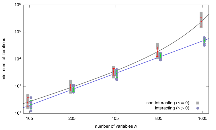
Figure 7: Replicated Simulated Annealing on the fully-connected committee machine, with $K=5$ hidden units, comparison between the interacting version (i.e. which seeks regions of high solution density) and the non-interacting version (i.e. standard SA), at $\alpha=0.2$ using $y=3$ replicas. This is the analogous of figure 2 of the main text for a committee machine, showing similar results. $10$ samples were tested for each value of $N$ (the same samples were used for the two curves). The bars represent averages and standard deviations (taken in logarithmic scale) while the lines represent fits. The interacting case was fitted by a function $aN^{b}$ with $a\simeq 0.02$, $b\simeq 2.0$, while the non-interacting case was fitted by a function $aN^{b}e^{cN^{d}}$ with $a\simeq 0.08$, $b\simeq 1.7$, $c\simeq 4.2\cdot 10^{-5}$, $d\simeq 1.5$. The two data sets are slightly shifted relative to each other for presentation purposes.

Appendix C Replicated Gradient Descent

C.1 Gradient computation

As mentioned in the main text, we perform a stochastic gradient descent on binary networks using the energy function of eq. (9) by using two sets of variables: a set of continuous variables $\mathcal{W}_{i}^{k}$ and the corresponding binarized variables $W_{i}^{k}$, related by $W_{i}^{k}=\operatorname*{sign}\left(\mathcal{W}_{i}^{k}\right)$. We use the binarized variables to compute the energy and the gradient, and apply the gradient to the continuous variables. In formulas, the quantities at time $t+1$ are related to those at time $t$ by:

$$\left(\mathcal{W}_{i}^{k}\right)^{t+1} = \left(\mathcal{W}_{i}^{k}\right)^{t}-\eta\frac{1}{\left|m\left(t\right)\right|}\sum_{\mu\in m\left(t\right)}\frac{\partial}{\partial W_{i}^{k}}E^{\mu}\left(W^{t}\right)$$ (34)

$$\left(W_{i}^{k}\right)^{t+1} = \operatorname*{sign}\left(\left(\mathcal{W}_{i}^{k}\right)^{t+1}\right)$$ (35)

where $\eta$ is a learning rate and $m\left(t\right)$ is a set of pattern indices (a so-called minibatch). A particularly simple scenario can be obtained by considering a single layer network without replication ($K=1$, $y=1$) and a fixed learning rate, and by computing the gradient one pattern at a time ($\left|m\left(t\right)\right|=1$). In that case, $E^{\mu}\left(W\right)=R\left(-\sum_{i}W_{i}\xi_{i}^{\mu}\right)$ where $R\left(x\right)=\frac{1}{2}\left(x+1\right)\Theta\left(x\right)$ and the gradient is $\partial_{W_{i}}E^{\mu}\left(W\right)=-\frac{1}{2}\xi_{i}^{\mu}\Theta\left(-\sum_{i}W_{i}\xi_{i}^{\mu}\right)$. Since the relation (35) is scale-invariant, we can just set $\eta=4$ and obtain

$$\mathcal{W}_{i}^{t+1} = \mathcal{W}_{i}^{t}-2\xi_{i}^{\mu}\Theta\left(-\sum_{i}W_{i}^{t}\xi_{i}^{\mu}\right)$$ (36)

where now the auxiliary quantities $\mathcal{W}$ are discretized: if they are initialized as odd integers, they remain odd integers throughout the learning process. This is the so-called “Clipped Perceptron” (CP) rule, which is the same as the Perceptron rule (“in case of error, update the weights in the direction of the pattern, otherwise do nothing”) except that the weights are clipped upon usage to make them binary. Notably, the CP rule by itself does not scale well with $N$; it is however possible to make it efficient (see baldassi-et-all-pnas ; baldassi-2009 ).

In the two-layer case ($K>1$) the computation of the gradient is more complicated; it is however simpler than the computation of the energy shift which was necessary for Simulated Annealing (Algorithm 1), since we only consider infinitesimal variations when computing the gradient. The resulting expression is:

$$\partial_{W_{i}^{k}}E^{\mu}\left(W\right)=\begin{cases}-\frac{1}{2}\xi_{i}^{k\mu}&\mathrm{if\>}\left(\Delta_{\mathrm{out}}^{\mu}<0\right)\wedge\left(1+2s_{c^{\mu}}^{\mu}\leq\Delta_{k}^{\mu}<0\right)\\ 0&\mathrm{otherwise}\end{cases}$$ (37)

i.e. the gradient is non-zero only in case of error, and only for those units $k$ which contribute to the energy computation (which turn up in the first $c^{\mu}$ terms of the sorted vector $s^{\mu}$, see eqs. (10)-(13)). Again, since this gradient can take only $3$ possible values, we could set $\eta=4$ and use discretized odd variables for the $\mathcal{W}$.

It is interesting to point out that a slight variation of this update rule in which only the first, least-wrong unit is affected, i.e. in which the condition $\left(1+2s_{c^{\mu}}^{\mu}\leq\Delta_{k}^{\mu}\right)$ is changed to $\left(1+2s_{1}^{\mu}\leq\Delta_{k}^{\mu}\right)$, was used in baldassi_subdominant_2015 , giving good results on a real-world learning task when a slight modification analogous to the one of baldassi-2009 was added. Note that, in the later stages of learning, when the overall energy is low, it is very likely that $c^{\mu}\leq 1$, implying that the simplification used in baldassi_subdominant_2015 likely has a negligible effect. The simplified version, when used in the continuous case, also goes under the name of “least action” algorithm mitchison1989bounds .

Having computed the gradient of $E\left(W\right)$ for each system, the extension to the replicated system is rather straightforward, since the energy (with the traced-out center) becomes (cf. eqs. (4) and (5) in the main text):

$$H\left(\left\{W^{a}\right\}\right)=\sum_{a=1}^{y}E\left(W^{a}\right)-\frac{1}{\beta}\sum_{j=1}^{N}\log\left(e^{-\frac{\gamma}{2}\sum_{a=1}^{y}\left(W_{j}^{a}-1\right)^{2}}+e^{-\frac{\gamma}{2}\sum_{a=1}^{y}\left(W_{j}^{a}+1\right)^{2}}\right)$$ (38)

and therefore the gradient just has an additional term:

$$\frac{\partial H}{\partial W_{i}^{a}}\left(\left\{W^{b}\right\}\right)=\left.\frac{\partial E}{\partial W_{i}}\left(W\right)\right|_{W=W^{a}}-\frac{\gamma}{\beta}\left(\tanh\left(\gamma\sum_{b=1}^{y}W_{i}^{b}\right)-W_{i}^{a}\right)$$ (39)

Note that the trace operation brings the parameter $\beta$ into account. Using $\eta^{\prime}=\frac{\gamma}{\beta\eta}$ as control parameter, the update equation (34) for a replica $a$ becomes (we omit the unit index $k$ for simplicity):

$$\left(\mathcal{W}_{i}^{a}\right)^{t+1} = \left(\mathcal{W}_{i}^{a}\right)^{t}-\eta\frac{1}{\left|m\left(t\right)\right|}\sum_{\mu\in m\left(t\right)}\left.\frac{\partial E^{\mu}}{\partial W_{i}}\left(W\right)\right|_{W=\left(W^{a}\right)^{t}}+\eta^{\prime}\left(\tanh\left(\gamma\sum_{b=1}^{y}\left(W_{i}^{b}\right)^{t}\right)-\left(W_{i}^{a}\right)^{t}\right)$$ (40)

In the limit $\beta,\gamma\to\infty$, $\eta^{\prime}$ stays finite, while the $\tanh$ reduces to a $\operatorname*{sign}$.

The expression of eq. (40) is derived straightforwardly, gives good results and is the one that we have used in the tests shown in the main text and below. It could be noted, however, that the two-level precision of the variables used in the algorithm introduces some artifacts. As a clear example, in the case of a single replica ($y=1$) or, more in general, when the replica indices $W_{i}^{a}$ are all aligned, we would expect the interaction term to vanish, while this is not the case except at $\gamma=\infty$.

One possible way to fix this issue is the following: we can introduce a factor in the logarithm in expression (38):

$$\log\left(\frac{e^{-\frac{\gamma}{2}\sum_{a=1}^{y}\left(W_{j}^{a}-1\right)^{2}}+e^{-\frac{\gamma}{2}\sum_{a=1}^{y}\left(W_{j}^{a}+1\right)^{2}}}{f\left(W_{j}^{1},\dots,W_{j}^{y}\right)}\right)$$ (41)

such that $f\left(W_{j}^{1},\dots,W_{j}^{y}\right)=1$ whenever its arguments lie on the vertices of the hypercube, $W_{j}^{a}\in\left\{-1,1\right\}$. This does not change the Hamiltonian for the configurations we’re interested in, but it can change its gradient. We can thus impose the additional constraint that the derivative of the above term vanishes whenever the $W_{j}^{a}$ are all equal. There are several ways to achieve this; however, if we assume that the function $f$ has the general structure

$$f\left(W_{j}^{1},\dots,W_{j}^{y}\right)=a\left(g\left(W_{j}^{1}\right),\dots,g\left(W_{j}^{y}\right)\right)$$ (42)

with $g\left(1\right)=g\left(-1\right)$ and with $a\left(\dots\right)$ being a totally symmetric function of its arguments, then it can be easily shown that necessarily

$$\frac{\partial}{\partial W_{i}^{a}}\log\left(\frac{e^{-\frac{\gamma}{2}\sum_{b=1}^{y}\left(W_{j}^{b}-1\right)^{2}}+e^{-\frac{\gamma}{2}\sum_{b=1}^{y}\left(W_{j}^{b}+1\right)^{2}}}{a\left(g\left(W_{j}^{1}\right),\dots,g\left(W_{j}^{y}\right)\right)}\right)=\gamma\left(\tanh\left(\gamma\sum_{b=1}^{y}W_{i}^{b}\right)-\tanh\left(\gamma y\right)W_{i}^{a}\right)$$ (43)

This expression has now two zeros corresponding to the fully aligned configurations of the weights at $+1$ and $-1$, as desired, and is a very minor correction of the original one used in eq. (40) (the expressions become identical at large values of $\gamma y$). In fact, we found that the numerical results are basically the same (the optimal values of the parameters may change, but the performances for optimal parameters are very similar for the two cases), such that this correction is not needed in practice.

An alternative, more straightforward way to fix the issue of the non-vanishing gradient with aligned variables is to perform the trace over the reference configurations in the continuous case (i.e. replacing the sum over the binary hypercube with an integral). This leads to the an expression for the interaction contribution to the gradient of this form: $\gamma\left(\frac{1}{y}\sum_{b=1}^{y}W_{i}^{b}-W_{i}^{a}\right)$. This, however, does seem to have a very slightly but measurably worse overall performance with respect to the previous ones (while still dramatically outperforming the non-interacting version).

In general, the tests with alternative interaction terms show that, despite the fact that the two-level gradient procedure is purely heuristic and inherently problematic, the fine details of the implementation may not be exceedingly relevant for most practical purposes.

The code for our implementation is available at codeRSGD .

C.2 Numerical simulations details

Our implementation of the formula in eq. (40) follows this scheme: at each time step, we have the values $T_{i}=\sum_{b=1}^{y}W_{i}^{b}$, we pick a random replica index $a$, compute the gradient with respect to some $m\left(t\right)$ patterns, update the values $\mathcal{W}^{a}$ and $W^{a}$, compute the gradient with respect to the interaction term using $T$ and $W^{a}$, and update the values of $T$ and – again – of $\mathcal{W}^{a}$ and $W^{a}$. This scheme is thus easy to parallelize, since it alternates the standard learning periods in which each replica acts independently with brief interaction periods in which the sum $T$ is updated, similarly to what was done in NIPS2015_5761 .

An epoch consists of a presentation of all patterns to all replicas. The minibatches $m\left(t\right)$ are randomized at the beginning of each epoch, independently for each replica. The replicas were initialized equally for simplicity.

In our tests, we kept fixed the learning rates $\eta$ and $\eta^{\prime}$ during the training process, since preliminary tests did not show a benefit in adapting them dynamically in our setting. We did, however, find beneficial in most cases to vary $\gamma,$ starting at some value $\gamma_{0}$ and increasing it progressively by adding a fixed quantity $d\gamma$ after each epoch, i.e. implementing a “scoping” mechanism as in the Simulated Annealing case (although even just using $\gamma=\infty$ from the start already gives large improvements against the non-interacting version).

All tests were capped at a maximum of $10^{4}$ epochs, and the minimum value of the error across all replicas was kept for producing the graphs.

In the interacting case, we systematically tested various values of $\eta^{\prime}$, $\gamma_{0}$ and $d\gamma$, and, for each $\alpha$, we kept the ones which produced optimal results (i.e. lowest error rate, or shorter solution times if the error rates were equal) on average across the samples. Because of the overall scale invariance of the problem, we did not change $\eta$.

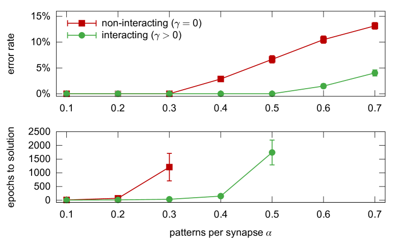
Figure 8: Replicated Stochastic Gradient descent on a fully-connected committee machine with $N=1605$ synapses and $K=5$ units in the second layer, comparison between the non-interacting (i.e. standard SGD) and interacting versions, using $y=3$ replicas and a minibatch size of $10$ patterns. Each point shows averages and standard deviations on $10$ samples with optimal choice of the parameters, as a function of the training set size. Top: minimum training error rate achieved after $10^{4}$ epochs. Bottom: number of epochs required to find a solution. Only the cases with $100\%$ success rate are shown.

Figure 8 shows the results of the same tests as shown in figure 3 of the main text for different values of the number of replicas and the minibatch size. The results for the interacting case are slightly worse, but still much better than for the non-interacting case.

For the perceptron case $K=1$ we did less extensive tests; we could solve $10$ samples out of $10$ with $N=1601$ synapses at $\alpha=0.7$ in an average of $4371\pm 661$ epochs with $y=7$ replicas and a minibatch size of $80$ patterns.

Appendix D Replicated Belief Propagation

D.1 Belief Propagation implementation notes

Belief Propagation (BP) is an iterative message passing algorithm that can be used to derive marginal probabilities on a system within the Bethe-Peierls approximation mackay2003information ; yedidia2005constructing ; mezard_information_2009 . The messages $P_{j\to\mu}\left(\sigma_{j}\right)$ (from variable node $j$ to factor node $\mu$) and $P_{\mu\to j}\left(\sigma_{j}\right)$ (from factor node $a$ to variable node $j$) represent cavity probability distributions (called messages) over a single variable $\sigma_{j}$. In the case of Ising systems of binary $\pm 1$ variables like the ones we are using in the network models considered in this work, the messages can be represented as a single number, usually a magnetization $m_{i\to\mu}=P_{i\to\mu}\left(+1\right)-P_{\mu\to i}\left(-1\right)$ (and analogous for the other case).

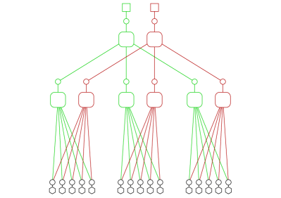
(a) BP factor graph scheme. This scheme exemplifies a factor graph for a committee machine with $N=15$ variables, $K=3$ units in the second layer, trained on $2$ patterns. The two patterns are distinguished by different colors. The graph can represent a fully-connected committee machine if the patterns are the same for all first-layer units, or a tree-like one if they are different. The variable nodes are represented as circles, the interaction by other geometrical figures. The hexagons at the bottom represent pseudo-self-interaction nodes (see main text, figure 4), the large squares with rounded corners represent perceptron-like nodes, the small squares at the top represent external fields enforcing the desired output of the machine. The synaptic variables $W_{j}^{k}$ are at the bottom (black circles), while the rest of the variables are auxiliary and represent the output of each unit for a given pattern.

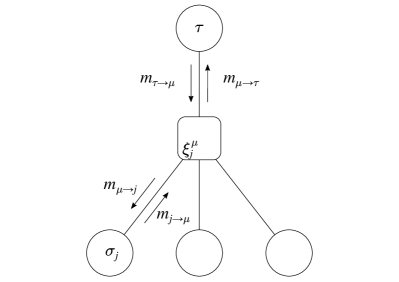
(b) BP messages naming scheme used in section D.1 for a perceptron-like factor node. The node $\mu$ is represented by the central square. Input variables, denoted by $\sigma_{j}$, are at the bottom. The output variable is called $\tau$. The couplings $\xi_{j}^{\mu}$ parametrize the factor node (one parameter per input edge) and can either represent an input pattern (for the first layer of the network) or be $1$ (for the second layer of the network).

Figure 9:

Our implementation of BP on binary networks follows very closely that of braunstein-zecchina , since we only consider the zero temperature case and we are interested in the “satisfiable” phase, thus considering only configurations of zero energy. However, in order to avoid some numerical precision issues that affected the computations at high values of $\alpha$, $y$ and $\gamma$, we lifted some of the approximations used in that paper. Here therefore we recapitulate the BP equations used and highlight the differences with the previous work. The factor graph scheme for a committee machine is shown for reference in figure 9a. The BP equations for the messages from a variable node $j$ to a factor node $\mu$ can be written in general as:

$$m_{j\to\mu}^{t} = \tanh\left(\sum_{\nu\in\partial j\setminus\mu}\tanh^{-1}\left(m_{\nu\to j}^{t}\right)+\tanh^{-1}\left(m_{\star\to j}^{t}\right)\right)$$ (44)

where $\partial j$ represent the set of all factor nodes in which variable $j$ is involved. This expression includes the Focusing BP (fBP) extra message $m_{\star\to j}$ described in the main text. The general expression for perceptron-like factor nodes is considerably more complicated. For the sake of generality, here we will use the symbol $\sigma$ to denote input variables of the node (with subscript $j$ indicating the variable), and $\tau$ for the output variable. To each perceptron-like factor $\mu$ is associated a vector of couplings $\xi^{\mu}$: in a committee-machine, these represent the patterns for the first layer nodes, and are simply vectors of ones in the second layer. See figure 9b.

Let us define the auxiliary functions:

$$\mathrm{f}_{j}^{\mu}\left(\left\{m_{i\to\mu}\right\}_{i\in\partial\mu\setminus j},m_{\tau\to\mu},\sigma_{j}\right) = \sum_{\tau,\sigma_{\partial\mu\setminus j}}\!\left(\frac{1+\tau\,m_{\tau\to\mu}}{2}\right)\Theta\negthinspace\left(\tau\left(\sum_{i\in\partial\mu\setminus j}\xi_{i}^{\mu}\sigma_{i}+\xi_{j}^{\mu}\sigma_{j}\right)\!\!\right)\!\prod_{i\in\partial\mu\setminus j}\left(\frac{1+\sigma_{i}m_{i\to\mu}}{2}\right)$$ (45)

$$\mathrm{f}^{\mu}\left(\left\{m_{i\to\mu}\right\}_{i\in\partial\mu},\tau\right) = \sum_{\sigma_{\partial\mu\setminus j}}\Theta\left(\tau\left(\sum_{i\in\partial\mu}\xi_{i}^{\mu}\sigma_{i}\right)\right)\prod_{i\in\partial\mu}\left(\frac{1+\sigma_{i}m_{i\to\mu}}{2}\right)$$ (46)

where $\partial\mu$ represents the set of all input variables involved in node $\mu$, $\sigma_{\partial\mu}=\left\{\sigma_{i}\right\}_{i\in\partial\mu}$ the configuration of input variables involved in node $\mu$, $m_{\tau\to\mu}$ the message from the output variable $\tau$ to the node $\mu$ (see figure 9b for reference). With these, the messages from factor node $\mu$ to the output variable node $\tau$ can be expressed as:

$$m_{\mu\to\tau}^{t+1}=\frac{\mathrm{f}^{\mu}\left(\left\{m_{i\to\mu}^{t}\right\}_{i\in\partial\mu},+1\right)-\mathrm{f}^{\mu}\left(\left\{m_{i\to\mu}^{t}\right\}_{i\in\partial\mu},-1\right)}{\mathrm{f}^{\mu}\left(\left\{m_{i\to\mu}^{t}\right\}_{i\in\partial\mu},+1\right)+\mathrm{f}^{\mu}\left(\left\{m_{i\to\mu}^{t}\right\}_{i\in\partial\mu},-1\right)}$$ (47)

while the message from factor node $\mu$ to input variable node j is:

$$m_{\mu\to j}^{t+1}=\frac{\mathrm{f}_{j}^{\mu}\left(\left\{m_{i\to\mu}^{t}\right\}_{i\in\partial\mu\setminus j},m_{\tau\to\mu}^{t},+1\right)-\mathrm{f}_{j}^{\mu}\left(\left\{m_{i\to\mu}^{t}\right\}_{i\in\partial\mu\setminus j},m_{\tau\to\mu}^{t},-1\right)}{\mathrm{f}_{j}^{\mu}\left(\left\{m_{i\to\mu}^{t}\right\}_{i\in\partial\mu\setminus j},m_{\tau\to\mu}^{t},+1\right)+\mathrm{f}_{j}^{\mu}\left(\left\{m_{i\to\mu}^{t}\right\}_{i\in\partial\mu\setminus j},m_{\tau\to\mu}^{t},-1\right)}$$ (48)

These functions can be computed exactly in $\mathcal{O}\left(N^{3}\right)$ operations, where $N$ is the size of the input, using either a partial convolution scheme or discrete Fourier transforms. When $N$ is sufficiently large, it is also possible to approximate them in $O\left(N\right)$ operations using the central limit theorem, as explained in braunstein-zecchina . In our tests on the committee machine, due to our choice of the parameters, we used the approximated fast version on the first layer and the exact version on the much smaller second layer.

In the fast approximated version, eqs. (47) and (48) become:

$$m_{\mu\to\tau}^{t+1} = \operatorname*{erf}\left(\frac{a_{\mu}^{t}}{\sqrt{2b_{\mu}^{t}}}\right)$$ (49)

$$m_{\mu\to j}^{t+1} = m_{\tau\to\mu}^{t}\frac{\mathrm{g}_{\mu\to j}^{t}\left(+1\right)-\mathrm{g}_{\mu\to j}^{t}\left(-1\right)}{2+m_{\tau\to\mu}^{t}\left(\mathrm{g}_{\mu\to j}^{t}\left(+1\right)+\mathrm{g}_{\mu\to j}^{t}\left(-1\right)\right)}$$ (50)

where we have defined the following quantities:

$$a_{\mu}^{t} = \sum_{i\in\partial\mu}\xi_{i}^{\mu}m_{i\to\mu}^{t}$$ (51)

$$b_{\mu}^{t} = \sum_{i\in\partial\mu}\left(1-\left(m_{i\to\mu}^{t}\right)^{2}\right)$$ (52)

$$\mathrm{g}_{\mu\to j}^{t}\left(\sigma\right) = \operatorname*{erf}\left(\frac{a_{\mu\to j}^{t}+\sigma\xi_{j}^{\mu}}{\sqrt{2\left(b_{\mu\to j}^{t}\right)}}\right)$$ (53)

$$a_{\mu\to j}^{t} = a_{\mu}^{t}-\xi_{j}^{\mu}m_{j\to\mu}^{t}$$ (54)

$$b_{\mu\to j}^{t} = b_{\mu}^{t}-\left(1-\left(m_{j\to\mu}^{t}\right)^{2}\right)$$ (55)

In braunstein-zecchina , eq. (50) was approximated with a more computationally efficient expression in the limit of large $N$. We found that this approximation leads to numerical issues with the type of architectures which we used in our simulation at large values of $\alpha,$ $y$ and $\gamma$. For the same reason, it is convenient to represent all messages internally in “field representation” as was done in braunstein-zecchina , i.e. using $h_{\mu\to j}=\tanh^{-1}\left(m_{\mu\to j}\right)$ (and analogous expressions for all messages); furthermore, some expressions need to be treated specially to avoid numerical precision loss. For example, computing $h_{\mu\to\tau}$ according to eq. (49) requires the computation of an expression of the type $\tanh^{-1}\left(\operatorname*{erf}\left(x\right)\right)$, which, when computed naïvely with standard 64-bit IEEE floating point machine numbers and using standard library functions, rapidly loses precision at moderate-to-large values of the argument, thus requiring us to write a custom function to avoid this effect. The same kind of treatment is necessary throughout the code, particularly when computing the thermodynamic functions.

The code for our implementation is available at codeFBP .

After convergence, the single-site magnetizations can be computed as:

$$m_{j} = \tanh\left(\sum_{\nu\in\partial j}\tanh^{-1}\left(m_{\nu\to j}\right)+\tanh^{-1}\left(m_{\star\to j}\right)\right)$$ (56)

and the average overlap between replicas (plotted in Fig. 5) as:

$$q=\frac{1}{N}\sum_{j}m_{j}^{2}$$ (57)

The local entropy is computed from the entropy of the whole replicated system from the BP messages at their fixed point, as usually done within the Bethe-Peierls approximation, minus the entropy of the reference variables. The result is then divided by the number of variables $N$ and of replicas $y$. (This procedure is equivalent to taking the partial derivative of the free energy expression with respect to $y$.) Finally, we take a Legendre transform by subtracting the interaction term $\gamma S$, where $S$ is the estimated overlap between each replica’s weights and the reference:

$$S=\frac{1}{N}\sum_{j}\frac{m_{j\to\star}m_{\star\to j}+\tanh\left(\gamma\right)}{1+m_{j\to\star}m_{\star\to j}\tanh\left(\gamma\right)}$$ (58)

From $S$, the distance between the replicas and the reference is simply computed as $\left(1+S\right)/2$.

D.2 Focusing BP vs Reinforced BP

As mentioned in the main text, the equation for the pseudo-self-interaction of the replicated Belief Propagation algorithm (which we called “Focusing BP”, fBP) is (eq. (7) in the main text):

$$m_{\star\to j}^{t+1}=\tanh\left(\left(y-1\right)\tanh^{-1}\left(m_{j\to\star}^{t}\tanh\gamma\right)\right)\tanh\gamma$$ (59)

See also figure 4 in the main text for a graphical description. The analogous equation for the reinforcement term which has been used in several previous works is (eq. (8) in the main text):

$$m_{\star\to j}^{t+1}=\tanh\left(\rho\tanh^{-1}\left(m_{j}^{t}\right)\right)$$ (60)

The reinforced BP has traditionally been used as follows: the reinforcement parameter $\rho$ is changed dynamically, starting from $0$ and increasing it up to $1$ in parallel with an ongoing BP message-passing iteration scheme. Therefore, in this approach, the BP messages can only converge (when $\rho=1$) to a completely polarized configuration, i.e. one where $m_{j}\in\left\{-1,+1\right\}$ for all $j$.

The same approach can be applied with the fBP scheme, except that eq. (59) involves two parameters, $\gamma$ and $y$, rather than one, and both need to diverge in order to ensure that the marginals $m_{j}$ become completely polarized as well.

In this scheme, however, it is unclear how to compare directly the two equations, since in eq. (59) the self-reinforcing message $m_{\star\to j}$ is a function of a cavity marginal $m_{j\to\star}$, while in eq. (60) it is a function of a non-cavity marginal $m_{j}$. In order to understand the relationship between the two, we take a different approach: we assume that the parameters involved in the two update schemes ($\gamma$ and $y$ on one side, $\rho$ on the other) are fixed until convergence of the BP messages. In that case, one can then remove the time index $t$ from eqs. (59),(60) and obtain a self-consistent condition between the quantities $m_{\star\to j}$, $m_{j\to\star}$ and $m_{j}$ at the fixed point:

$$m_{j}=\tanh\left(\tanh^{-1}\left(m_{\star\to j}\right)+\tanh^{-1}\left(m_{j\to\star}\right)\right)$$ (61)

Therefore eq. (60) in this case becomes equivalent to:

$$m_{j}=\tanh\left(\frac{1}{1-\rho}\tanh^{-1}\left(m_{j\to\star}\right)\right)$$ (62)

to be compared with the analogous expression for the fBP case:

$$m_{j}=\tanh\left(\tanh^{-1}\left(m_{j\to\star}\right)+\tanh^{-1}\left(\tanh\left(\left(y-1\right)\tanh^{-1}\left(m_{j\to\star}\tanh\gamma\right)\right)\tanh\gamma\right)\right)$$ (63)

This latter expression is clearly much more complicated, but by letting $\gamma\to\infty$ and setting $y=\frac{1}{1-\rho}$ it simplifies to eq. (62). Therefore, we have an exact mapping between fBP and the reinforced BP. The interpretation of this mapping in terms of the reweighted entropic measure (eq. (II) of the main text) is not straightforward, because of the requirement $\gamma=\infty$. The $\gamma=\infty$ case at finite $y$ is an extreme case: as mentioned in the main text, the BP equations applied to the replicated factor graph (figure 4 of the main text) neglect the correlations between the messages $m_{\star\to j}$ targeting different replicas. Since as $\gamma\to\infty$ these messages become completely correlated, the approximation fails. As demonstrated by our results, though (figures 5 and 6 in the main text, and figure 11 below), this failure in the approximation only happens at very large values of $\gamma$, and its onset is shifted to larger values of $\gamma$ as $y$ is increased, so that even keeping $y$ fixed (but sufficiently large) and gradually increasing $\gamma$ gives very good results (figure 6 in the main text). A different approach to the interpretation of the reinforcement protocol is instead to consider that it is only one among several possible protocols. As we showed in the main text for the case of the committee machine, even keeping $y$ fixed (but sufficiently large) and gradually increasing $\gamma$ gives very good results. One possible generalization, in which both $\gamma$ and $y$ start from low values and are progressively increased, we can consider:

$$\gamma = \tanh^{-1}\left(\rho^{x}\right)$$ (64)

$$y = 1+\frac{\rho^{1-2x}}{\left(1-\rho\right)}$$ (65)

The second expression was obtained by assuming the first one and matching the derivative of the curves of eqs. (62) and (63) in the point $m_{j\to\star}=0$. Note that with this choice, both $\gamma\to\infty$ and $y\to\infty$ in the limit $\rho\to 1$, thus ensuring that, in that limit, the only fixed points of the iterative message passing procedure are completely polarized, and consistently with the notion that we are looking regions of maximal density ($y\to\infty$) at small distances ($\gamma\to\infty$). When setting $x=0$, this reproduces the standard reinforcement relations. However, other values of $x$ produce the same qualitative behavior, and are quantitatively very similar: figure (10) shows the comparison with the case $x=0.5$. In practice, in our tests these protocols have proved to be equally effective in finding solutions of the learning problem.

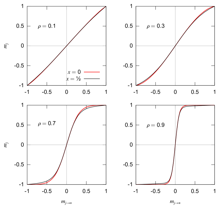
Figure 10: Plots of eq. (63), comparison of protocols defined by eqs. (65) and (64) with two different values of the parameter $x$. The $x=0$ case (thick red lines) corresponds to standard reinforcement. The curves are in fact very similar across the whole range of $\rho\in\left[0,1\right]$ and $x\in\left[0,1\right]$, and consequently display similar performance properties in practice.

D.3 Focusing BP vs analytical results

Figure 11: Comparison of local entropy curves between the fBP results and the analytical predictions, for the case of the perceptron with $\alpha=0.6$. The algorithmic results (blue curve) were obtained with $N=1001$ at $y=21$, averaging over $50$ samples. Error bars indicate the estimated standard deviation of the mean. The RS results (red curve) were also obtained with $y=21$. The 1RSB results, however, are for the $y=\infty$ case, and it is therefore to be expected that the corresponding curve is slightly higher.

We compared the local entropy curves produced with the fBP algorithm on perceptron problems with the RS and 1RSB results obtained analytically in baldassi_subdominant_2015 ; baldassi2016learning . We produced curves at fixed $y$ and $\alpha$, while varying $\gamma$. However, we only have 1RSB results for the $y=\infty$ case. Figure 11 shows the results for $\alpha=0.6$ and $y=21$, demonstrating that the fBP curve deviates from the RS prediction and is very close to the 1RSB case. Our tests show that the fBP curve get closer to the 1RSB curve as $y$ grows. This analysis confirms a scenario in which the fBP algorithm spontaneously choses a high density state, breaking the symmetry in a way which seems to approximate well the 1RSB description. Numerical precision issues limited the range of parameters that we could explore in a reasonable time.

D.4 Focusing BP on random $K$-SAT

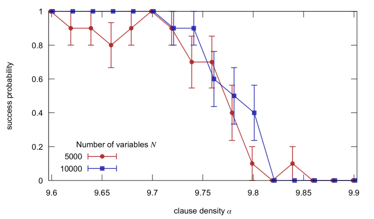
Figure 12: Probability of finding a solution in random instances of $4$-SAT as a function of clause density $\alpha$ using the fBP algorithm described in the text. The results are shown for two values of $N$, slightly shifted relative to each other to improve readability. The points and error bars represent averages and standard deviations over $10$ samples.

In this section, we show how to apply the Focusing BP (fBP) scheme on a prototypical constraint statisfaction problem, the random $K$-satisfiability ($K$-SAT) problem mezard_information_2009 , and present the results of some preliminary experiments in which it is used as a solver algorithm.

An instance of $K$-SAT is defined by $N$ variables and $M$ clauses, each clause $\mu$ involving $K$ variables indexed in $\partial\mu\subseteq\left\{1,\dots,N\right\}$, $\left|\partial\mu\right|=K$. We call $\alpha=M/N$ the clause density. In the notation of this section, variables are denoted by $\sigma_{i}$, $i=1,\dots,N$, and take values in $\left\{-1,+1\right\}$. To each clause $\mu$ is associated a set of couplings, one for each variable in $\partial\mu$. The coupling $J_{\mu i}$ takes the value $-1$ if the variable $i$ is negated in clause $\mu$, and $+1$ otherwise. A configuration $\left\{\sigma_{i}\right\}_{i=1}^{N}$ satisfies the clause $\mu$ if $\exists i\in\partial\mu$ such that $J_{\mu i}=\sigma_{i}$. An instance of the problem is said to be satisfiable if there exists a configuration which satisfies all clauses. The Hamiltonian for this problem, which counts the number of violated clauses, is then given by:

$$H\left(\sigma\right)=\sum_{\mu=1}^{M}\prod_{i\in\partial\mu}\frac{1-J_{\mu i}\sigma_{i}}{2}.$$ (66)

Random instances of the problem are generated by sampling uniformly and independently at random the subsets $\partial\mu$ and choosing the couplings $J_{\mu i}$ independently in $\left\{-1,+1\right\}$ with equal probability. Random instances of $K$-SAT are locally tree-like in the large $N$ limit, therefore the problem is suitable to investigation through the tools of statistical physics of disordered systems, namely the cavity method mezard_information_2009 . Such investigation in fact led in the past decades to outstanding theoretical advances in understanding the structure of the problem mezard_information_2009 ; krzakala-csp and to devise state-of-the-art solvers braunstein2005survey .

In order to apply the cavity method to $K$-SAT one identifies each clause with a factor node and each variable with a variable node; it is then convenient to parametrize clauses-to-variables cavity messages with $P_{\mu\to i}\left(\sigma_{i}=J_{\mu i}\right)\equiv\eta_{\mu\to i}$, and variables-to-clauses ones with $P_{i\to\mu}\left(\sigma_{i}\neq J_{\mu i}\right)\equiv\zeta_{i\to\mu}.$ We also define the variables’ subsets $\partial^{+}i$ and $\partial^{-}i$ as $\partial^{\pm}i=\left\{\mu\in\partial i\ :\ J_{\mu i}=\pm 1\right\}$. With these definitions, the zero temperature BP update rules take the form:

$$\pi_{\pm,i\to\mu}^{t}= \tilde{\pi}_{\pm,i}^{t}\prod_{\nu\in\partial^{\pm}i\setminus\mu}\,\eta_{\nu\to i}^{t},$$ (67)

$$\zeta_{i\to\mu}^{t}= \frac{\pi_{J_{\mu i},i\to\mu}^{t}}{\pi_{+,i\to\mu}^{t}\ +\pi_{-,i\to\mu}^{t}},$$ (68)

$$\eta_{\mu\to i}^{t+1}= 1-\prod_{j\in\partial\mu\setminus i}\,\zeta_{j\to\mu}^{t}.$$ (69)

Magnetizations at time $t$ are given by:

$$m_{i}^{t}= \frac{\tilde{\pi}_{+,i}^{t}\prod_{\nu\in\partial^{+}i}\,\eta_{\nu\to i}^{t}\ -\ \tilde{\pi}_{-,i}^{t}\prod_{\nu\in\partial^{+}i}\,\eta_{\nu\to i}^{t}}{\tilde{\pi}_{+,i}^{t}\prod_{\nu\in\partial^{+}i}\,\eta_{\nu\to i}^{t}\ +\ \tilde{\pi}_{-,i}^{t}\prod_{\nu\in\partial^{+}i}\,\eta_{\nu\to i}^{t}}.$$ (70)

The update rules of the coefficients $\tilde{\pi}_{\pm,i}^{t}$ depend on the algorithm under consideration. In standard BP, the coefficients $\tilde{\pi}_{\pm,i}^{t}$ are set to:

$$\tilde{\pi}_{\pm,i}^{t}\equiv 1.$$ (71)

A common procedure for finding solutions for the $K$-SAT problem, called BP guided decimation (BPGD), consists in iterating Eqs. (67-69) until convergence; computing marginals according to Eq. (70); fixing a certain fraction of variables, the ones with most polarized marginals, to $\sigma_{i}=\mathrm{sgn}\left(m_{i}\right)$; repeating the procedure on the reduced problem, until a satisfying configuration is found or a contradiction is produced. (A contradiction occurs when all variables involved in a clause are fixed to values that violate the clause.)

We can avoid to irrevocably fix the variables at intermediate steps of the algorithm, as in BPGD, using instead the reinforced BP (rBP) heuristic, which acts as a “soft” decimation. For rBP the new update rule reads:

$$\tilde{\pi}_{\pm,i}^{t+1}=\left(\pi_{\pm,i}^{t}\right)^{\rho}.$$ (72)

In rBP, Eqs. (67-69) and (72) are iterated, while the coefficient $\rho$ is increased up to one. The algorithm stops when clamping the magnetizations gives a solution, or a contradiction is produced.

For fBP, instead, the update rules are derived from the robust ensemble and are similar to the ones for neural networks:

$$m_{i\to\star}^{t} =\frac{\prod_{\nu\in\partial^{+}i}\,\eta_{\nu\to i}^{t}\ -\ \prod_{\nu\in\partial^{+}i}\,\eta_{\nu\to i}^{t}}{\prod_{\nu\in\partial^{+}i}\,\eta_{\nu\to i}^{t}\ +\ \prod_{\nu\in\partial^{+}i}\,\eta_{\nu\to i}^{t}},$$ (73)

$$m_{\star\to i}^{t+1}= \tanh\left(\left(y-1\right)\tanh^{-1}\left(m_{i\to\star}^{t}\tanh\gamma\right)\right)\tanh\gamma,$$ (74)

$$\tilde{\pi}_{\pm,i}^{t+1} =1\pm m_{\star\to i}^{t+1}.$$ (75)

We performed some preliminary tests of the effectiveness of fBP as a solver in $K$-SAT (see Fig. 12), to be expanded in future investigations. We used the following protocol: we iterated Eqs. (67-69,73-75) at fixed $y=6$ and increasing $\gamma$ in steps of $0.01$ every $2000$ iterations, starting from $\gamma=0.01$. The algorithm is stopped when a solution is found (by clamping to $\pm 1$ the cavity marginals) or when $\gamma=0.6$ is reached without finding any solution. The BP update equations often converged to a fixed point before reaching $2000$ iterations, in which case we skipped to the next value of $\gamma$; in order to aid convergence, we added some damping to the iterative procedure.

We didn’t test extensively the possible heuristic schemes to turn fBP into an efficient solver, therefore there is surely room for improvement over the one adopted here. Nonetheless, our procedure—when successful—found solutions quite rapidly, even though it is not as fast as rBP. More importantly, it finds solutions up to high values of $\alpha$. Defining $\alpha_{d}=9.38$, $\alpha_{c}=9.547$ and $\alpha_{s}=9.93$ the dynamic, static and SAT/UNSAT transitions respectively in $4$-SAT krzakala-csp , from Fig. 12 it appears that the algorithmic threshold for fBP is $\alpha_{c}<\alpha_{fBP}<\alpha_{s}$. In comparison, BPGD starts to fail much earlier, $\alpha_{BPGD}\approx\alpha_{d}$ mezard_information_2009 . The fBP performance seems in fact to be rather close to that of the “Survey Propagation with Backtracking” algorithm of marino2015backtrackingSP (in particular, the curves in Fig. 1 in that paper can be directly compared and appear to be similar to those in Fig. 12 in the present paper), although a much more extensive and detailed analysis (like the one performed in marino2015backtrackingSP ) would be required in order to obtain a good estimate of the algorithmic threshold of fBP in the large $N$ limit.

References

- (1) Yann LeCun, Yoshua Bengio, and Geoffrey Hinton. Deep learning. Nature, 521(7553):436–444, 2015.
- (2) Jiquan Ngiam, Adam Coates, Ahbik Lahiri, Bobby Prochnow, Quoc V Le, and Andrew Y Ng. On optimization methods for deep learning. In Proceedings of the 28th International Conference on Machine Learning (ICML-11), pages 265–272, 2011.
- (3) Patrick Charbonneau, Jorge Kurchan, Giorgio Parisi, Pierfrancesco Urbani, and Francesco Zamponi. Fractal free energy landscapes in structural glasses. Nature communications, 5, 2014.
- (4) Federico Ricci-Tersenghi and Guilhem Semerjian. On the cavity method for decimated random constraint satisfaction problems and the analysis of belief propagation guided decimation algorithms. Journal of Statistical Mechanics: Theory and Experiment, 2009(09):P09001, 2009.
- (5) Paul C Bressloff. Stochastic processes in cell biology, volume 41. Springer, 2014.
- (6) David Easley and Jon Kleinberg. Networks, crowds, and markets: Reasoning about a highly connected world. Cambridge University Press, 2010.
- (7) Anthony Holtmaat and Karel Svoboda. Experience-dependent structural synaptic plasticity in the mammalian brain. Nature Reviews Neuroscience, 10(9):647–658, 2009.
- (8) Sixin Zhang, Anna E Choromanska, and Yann LeCun. Deep learning with elastic averaging sgd. In C. Cortes, N. D. Lawrence, D. D. Lee, M. Sugiyama, and R. Garnett, editors, Advances in Neural Information Processing Systems 28, pages 685–693. Curran Associates, Inc., 2015.
- (9) Accessible states in deep networks (preliminary title), C. Baldassi, C. Borgs, L. Bottou, J. Chayes, A. Ingrosso, Y. LeCun, C. Lucibello, L. Saglietti and R. Zecchina. in preparation, 2016.
- (10) Scott Kirkpatrick, Mario P Vecchi, et al. Optimization by simmulated annealing. science, 220(4598):671–680, 1983.
- (11) Marc Mézard, Giorgio Parisi, and Riccardo Zecchina. Analytic and algorithmic solution of random satisfiability problems. Science, 297(5582):812–815, 2002.
- (12) Florent Krzakala, Andrea Montanari, Federico Ricci-Tersenghi, Guilhem Semerjian, and Lenka Zdeborova. Gibbs states and the set of solutions of random constraint satisfaction problems. Proceedings of the National Academy of Sciences, 104(25):10318–10323, 2007.
- (13) Lenka Zdeborová and Marc Mézard. Locked constraint satisfaction problems. Phys. Rev. Lett., 101:078702, Aug 2008.
- (14) Carlo Baldassi, Alessandro Ingrosso, Carlo Lucibello, Luca Saglietti, and Riccardo Zecchina. Subdominant Dense Clusters Allow for Simple Learning and High Computational Performance in Neural Networks with Discrete Synapses. Physical Review Letters, 115(12):128101, September 2015.
- (15) Haiping Huang and Yoshiyuki Kabashima. Origin of the computational hardness for learning with binary synapses. Physical Review E, 90(5):052813, 2014.
- (16) Carlo Baldassi, Alessandro Ingrosso, Carlo Lucibello, Luca Saglietti, and Riccardo Zecchina. Local entropy as a measure for sampling solutions in constraint satisfaction problems. Journal of Statistical Mechanics: Theory and Experiment, 2016(2):P023301, February 2016.
- (17) Marc Mézard and Andrea Montanari. Information, Physics, and Computation. Oxford University Press, January 2009.
- (18) Carlo Baldassi, Federica Gerace, Carlo Lucibello, Luca Saglietti, and Riccardo Zecchina. Learning may need only a few bits of synaptic precision. Physical Review E, 93(5):052313, May 2016.
- (19) Cristopher Moore and Stephan Mertens. The nature of computation. Oxford University Press, 2011.
- (20) David E Rumelhart, Geoffrey E Hinton, and Ronald J Williams. Learning representations by back-propagating errors. Cognitive modeling, 5(3):1, 1988.
- (21) Sepp Hochreiter. Untersuchungen zu dynamischen neuronalen netzen. Master’s thesis, Institut fur Informatik, Technische Universitat, Munchen, 1991.
- (22) Carlo Baldassi, Alfredo Braunstein, Nicolas Brunel, and Riccardo Zecchina. Efficient supervised learning in networks with binary synapses. Proceedings of the National Academy of Sciences, 104:11079–11084, 2007.
- (23) Carlo Baldassi. Generalization learning in a perceptron with binary synapses. J. Stat. Phys., 136:902–916, 2009.
- (24) Yann LeCun, Léon Bottou, Yoshua Bengio, and Patrick Haffner. Gradient-based learning applied to document recognition. Proceedings of the IEEE, 86(11):2278–2324, 1998.
- (25) Matthieu Courbariaux, Yoshua Bengio, and Jean-Pierre David. Binaryconnect: Training deep neural networks with binary weights during propagations. In Advances in Neural Information Processing Systems, pages 3105–3113, 2015.
- (26) Itay Courbariaux, Matthieu Hubara, Daniel Soudry, Ran El-Yaniv, and Yoshua Bengio. Binarized neural networks: Training deep neural networks with weights and activations constrained to +1 or -1. arXiv preprint arXiv:1602.02830, 2016.
- (27) Implementation of the Replicated Stochastic Gradient Descent algorithm for binary committee machines. https://github.com/carlobaldassi/BinaryCommitteeMachineRSGD.jl.
- (28) Sixin Zhang. Distributed stochastic optimization for deep learning (thesis). arXiv preprint arXiv:1605.02216, 2016.
- (29) David JC MacKay. Information theory, inference and learning algorithms. Cambridge university press, 2003.
- (30) Jonathan S Yedidia, William T Freeman, and Yair Weiss. Constructing free-energy approximations and generalized belief propagation algorithms. Information Theory, IEEE Transactions on, 51(7):2282–2312, 2005.
- (31) Alfredo Braunstein and Riccardo Zecchina. Learning by message-passing in neural networks with material synapses. Phys. Rev. Lett., 96:030201, 2006.
- (32) Marc Bailly-Bechet, Christian Borgs, Alfredo Braunstein, J Chayes, A Dagkessamanskaia, J-M François, and Riccardo Zecchina. Finding undetected protein associations in cell signaling by belief propagation. Proceedings of the National Academy of Sciences, 108(2):882–887, 2011.
- (33) Yoshiyuki Kabashima. Replicated Bethe Free Energy: A Variational Principle behind Survey Propagation. Journal of the Physical Society of Japan, 74(8):2133–2136, aug 2005.
- (34) Implementation of the Focusing Belief Propagation algorithm for binary committee machines. https://github.com/carlobaldassi/BinaryCommitteeMachineFBP.jl.
- (35) Alfredo Braunstein, Luca Dall’Asta, Guilhem Semerjian, and Lenka Zdeborová. The large deviations of the whitening process in random constraint satisfaction problems. Journal of Statistical Mechanics: Theory and Experiment, 2016(5):053401, May 2016.
- (36) Raffaele Marino, Giorgio Parisi, and Federico Ricci-Tersenghi. The backtracking survey propagation algorithm for solving random K-SAT problems. http://arxiv.org/abs/1508.05117, 2015.
- (37) Luca Dall’Asta, Abolfazl Ramezanpour, and Riccardo Zecchina. Entropy landscape and non-gibbs solutions in constraint satisfaction problems. Physical Review E, 77(3):031118, 2008.
- (38) Carlo Baldassi. A method to reduce the rejection rate in Monte Carlo Markov Chains on Ising spin models. http://arxiv.org/abs/1608.05899, 2016.
- (39) GJ Mitchison and RM Durbin. Bounds on the learning capacity of some multi-layer networks. Biological Cybernetics, 60(5):345–365, 1989.
- (40) Alfredo Braunstein, Marc Mézard, and Riccardo Zecchina. Survey propagation: An algorithm for satisfiability. Random Structures & Algorithms, 27(2):201–226, 2005.