Structured Prediction Theory Based on
Factor Graph Complexity

Abstract

We present a general theoretical analysis of structured prediction with a series of new results. We give new data-dependent margin guarantees for structured prediction for a very wide family of loss functions and a general family of hypotheses, with an arbitrary factor graph decomposition. These are the tightest margin bounds known for both standard multi-class and general structured prediction problems. Our guarantees are expressed in terms of a data-dependent complexity measure, factor graph complexity, which we show can be estimated from data and bounded in terms of familiar quantities for several commonly used hypothesis sets along with a sparsity measure for features and graphs. Our proof techniques include generalizations of Talagrand’s contraction lemma that can be of independent interest.

We further extend our theory by leveraging the principle of Voted Risk Minimization (VRM) and show that learning is possible even with complex factor graphs. We present new learning bounds for this advanced setting, which we use to design two new algorithms, Voted Conditional Random Field (VCRF) and Voted Structured Boosting (StructBoost). These algorithms can make use of complex features and factor graphs and yet benefit from favorable learning guarantees. We also report the results of experiments with VCRF on several datasets to validate our theory.

1 Introduction

Structured prediction covers a broad family of important learning problems. These include key tasks in natural language processing such as part-of-speech tagging, parsing, machine translation, and named-entity recognition, important areas in computer vision such as image segmentation and object recognition, and also crucial areas in speech processing such as pronunciation modeling and speech recognition.

In all these problems, the output space admits some structure. This may be a sequence of tags as in part-of-speech tagging, a parse tree as in context-free parsing, an acyclic graph as in dependency parsing, or labels of image segments as in object detection. Another property common to these tasks is that, in each case, the natural loss function admits a decomposition along the output substructures. As an example, the loss function may be the Hamming loss as in part-of-speech tagging, or it may be the edit-distance, which is widely used in natural language and speech processing.

The output structure and corresponding loss function make these problems significantly different from the (unstructured) binary classification problems extensively studied in learning theory. In recent years, a number of different algorithms have been designed for structured prediction, including Conditional Random Field (CRF) (Lafferty et al., 2001), StructSVM (Tsochantaridis et al., 2005), Maximum-Margin Markov Network (M3N) (Taskar et al., 2003), a kernel-regression algorithm (Cortes et al., 2007), and search-based approaches such as (Daumé III et al., 2009; Doppa et al., 2014; Lam et al., 2015; Chang et al., 2015; Ross et al., 2011). More recently, deep learning techniques have also been developed for tasks including part-of-speech tagging (Jurafsky and Martin, 2009; Vinyals et al., 2015a), named-entity recognition (Nadeau and Sekine, 2007), machine translation (Zhang et al., 2008), image segmentation (Lucchi et al., 2013), and image annotation (Vinyals et al., 2015b).

However, in contrast to the plethora of algorithms, there have been relatively few studies devoted to the theoretical understanding of structured prediction (Bakir et al., 2007). Existing learning guarantees hold primarily for simple losses such as the Hamming loss (Taskar et al., 2003; Cortes et al., 2014; Collins, 2001) and do not cover other natural losses such as the edit-distance. They also typically only apply to specific factor graph models. The main exception is the work of McAllester (2007), which provides PAC-Bayesian guarantees for arbitrary losses, though only in the special case of randomized algorithms using linear (count-based) hypotheses.

This paper presents a general theoretical analysis of structured prediction with a series of new results. We give new data-dependent margin guarantees for structured prediction for a broad family of loss functions and a general family of hypotheses, with an arbitrary factor graph decomposition. These are the tightest margin bounds known for both standard multi-class and general structured prediction problems. For special cases studied in the past, our learning bounds match or improve upon the previously best bounds (see Section 3.3). In particular, our bounds improve upon those of Taskar et al. (2003). Our guarantees are expressed in terms of a data-dependent complexity measure, factor graph complexity, which we show can be estimated from data and bounded in terms of familiar quantities for several commonly used hypothesis sets along with a sparsity measure for features and graphs.

We further extend our theory by leveraging the principle of Voted Risk Minimization (VRM) and show that learning is possible even with complex factor graphs. We present new learning bounds for this advanced setting, which we use to design two new algorithms, Voted Conditional Random Field (VCRF) and Voted Structured Boosting (StructBoost). These algorithms can make use of complex features and factor graphs and yet benefit from favorable learning guarantees. As a proof of concept validating our theory, we also report the results of experiments with VCRF on several datasets.

The paper is organized as follows. In Section 2 we introduce the notation and definitions relevant to our discussion of structured prediction. In Section 3, we derive a series of new learning guarantees for structured prediction, which are then used to prove the VRM principle in Section 4. Section 5 develops the algorithmic framework which is directly based on our theory. In Section 6, we provide some preliminary experimental results that serve as a proof of concept for our theory.

2 Preliminaries

Let ${\mathcal{X}}$ denote the input space and ${\mathcal{Y}}$ the output space. In structured prediction, the output space may be a set of sequences, images, graphs, parse trees, lists, or some other (typically discrete) objects admitting some possibly overlapping structure. Thus, we assume that the output structure can be decomposed into $l$ substructures. For example, this may be positions along a sequence, so that the output space ${\mathcal{Y}}$ is decomposable along these substructures: ${\mathcal{Y}}={\mathcal{Y}}_{1}\times\cdots\times{\mathcal{Y}}_{l}$. Here, ${\mathcal{Y}}_{k}$ is the set of possible labels (or classes) that can be assigned to substructure $k$.

Loss functions. We denote by ${\mathsf{L}}\colon{\mathcal{Y}}\times{\mathcal{Y}}\to\mathbb{R}_{+}$ a loss function measuring the dissimilarity of two elements of the output space ${\mathcal{Y}}$. We will assume that the loss function ${\mathsf{L}}$ is definite, that is ${\mathsf{L}}(y,y^{\prime})=0$ iff $y=y^{\prime}$. This assumption holds for all loss functions commonly used in structured prediction. A key aspect of structured prediction is that the loss function can be decomposed along the substructures ${\mathcal{Y}}_{k}$. As an example, ${\mathsf{L}}$ may be the Hamming loss defined by ${\mathsf{L}}(y,y^{\prime})=\frac{1}{l}\sum_{k=1}^{l}1_{y_{k}\neq y^{\prime}_{k}}$ for all $y=(y_{1},\ldots,y_{l})$ and $y^{\prime}=(y^{\prime}_{1},\ldots,y^{\prime}_{l})$, with $y_{k},y^{\prime}_{k}\in{\mathcal{Y}}_{k}$. In the common case where ${\mathcal{Y}}$ is a set of sequences defined over a finite alphabet, ${\mathsf{L}}$ may be the edit-distance, which is widely used in natural language and speech processing applications, with possibly different costs associated to insertions, deletions and substitutions. ${\mathsf{L}}$ may also be a loss based on the negative inner product of the vectors of $n$-gram counts of two sequences, or its negative logarithm. Such losses have been used to approximate the BLEU score loss in machine translation. There are other losses defined in computational biology based on various string-similarity measures. Our theoretical analysis is general and applies to arbitrary bounded and definite loss functions.

Scoring functions and factor graphs. We will adopt the common approach in structured prediction where predictions are based on a scoring function mapping ${\mathcal{X}}\times{\mathcal{Y}}$ to $\mathbb{R}$. Let ${\mathcal{H}}$ be a family of scoring functions. For any $h\in{\mathcal{H}}$, we denote by ${\mathsf{h}}$ the predictor defined by $h$: for any $x\in{\mathcal{X}}$, ${\mathsf{h}}(x)=\operatorname*{argmax}_{y\in{\mathcal{Y}}}h(x,y)$.

Furthermore, we will assume, as is standard in structured prediction, that each function $h\in{\mathcal{H}}$ can be decomposed as a sum. We will consider the most general case for such decompositions, which can be made explicit using the notion of factor graphs. A factor graph $G$ is a tuple $G=(V,F,E)$, where $V$ is a set of variable nodes, $F$ a set of factor nodes, and $E$ a set of undirected edges between a variable node and a factor node. In our context, $V$ can be identified with the set of substructure indices, that is $V=\{1,\ldots,l\}$.

For any factor node $f$, denote by ${\mathscr{N}}(f)\subseteq V$ the set of variable nodes connected to $f$ via an edge and define ${\mathcal{Y}}_{f}$ as the substructure set cross-product ${\mathcal{Y}}_{f}=\prod_{k\in{\mathscr{N}}(f)}{\mathcal{Y}}_{k}$. Then, $h$ admits the following decomposition as a sum of functions $h_{f}$, each taking as argument an element of the input space $x\in{\mathcal{X}}$ and an element of ${\mathcal{Y}}_{f}$, $y_{f}\in{\mathcal{Y}}_{f}$:

$$h(x,y)=\sum_{f\in F}h_{f}(x,y_{f}).$$ (1)

Figure 1 illustrates this definition with two different decompositions. More generally, we will consider the setting in which a factor graph may depend on a particular example $(x_{i},y_{i})$: $G(x_{i},y_{i})=G_{i}=([l_{i}],F_{i},E_{i})$. A special case of this setting is for example when the size $l_{i}$ (or length) of each example is allowed to vary and where the number of possible labels $|{\mathcal{Y}}|$ is potentially infinite.

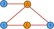
(a)	(b)

Figure 1: Example of factor graphs. (a) Pairwise Markov network decomposition: $h(x,y)=h_{f_{1}}(x,y_{1},y_{2})+h_{f_{2}}(x,y_{2},y_{3})$ (b) Other decomposition $h(x,y)=h_{f_{1}}(x,y_{1},y_{3})+h_{f_{2}}(x,y_{1},y_{2},y_{3})$.

We present other examples of such hypothesis sets and their decomposition in Section 3, where we discuss our learning guarantees. Note that such hypothesis sets ${\mathcal{H}}$ with an additive decomposition are those commonly used in most structured prediction algorithms (Tsochantaridis et al., 2005; Taskar et al., 2003; Lafferty et al., 2001). This is largely motivated by the computational requirement for efficient training and inference. Our results, while very general, further provide a statistical learning motivation for such decompositions.

Learning scenario. We consider the familiar supervised learning scenario where the training and test points are drawn i.i.d. according to some distribution ${\mathcal{D}}$ over ${\mathcal{X}}\times{\mathcal{Y}}$. We will further adopt the standard definitions of margin, generalization error and empirical error. The margin $\rho_{h}(x,y)$ of a hypothesis $h$ for a labeled example $(x,y)\in{\mathcal{X}}\times{\mathcal{Y}}$ is defined by

$$\rho_{h}(x,y)=h(x,y)-\max_{y^{\prime}\neq y}h(x,y^{\prime}).$$ (2)

Let $S=((x_{1},y_{1}),\ldots,(x_{m},y_{m}))$ be a training sample of size $m$ drawn from ${\mathcal{D}}^{m}$. We denote by $R(h)$ the generalization error and by $\widehat{R}_{S}(h)$ the empirical error of $h$ over $S$:

$$R(h)=\operatorname*{\mathbb{E}}_{(x,y)\sim{\mathcal{D}}}[{\mathsf{L}}({\mathsf{h}}(x),y)]\quad\text{ and }\quad\widehat{R}_{S}(h)=\operatorname*{\mathbb{E}}_{(x,y)\sim S}[{\mathsf{L}}({\mathsf{h}}(x),y)],$$ (3)

where ${\mathsf{h}}(x)=\operatorname*{argmax}_{y}h(x,y)$ and where the notation $(x,y)\!\!\sim\!\!S$ indicates that $(x,y)$ is drawn according to the empirical distribution defined by $S$. The learning problem consists of using the sample $S$ to select a hypothesis $h\in{\mathcal{H}}$ with small expected loss $R(h)$.

Observe that the definiteness of the loss function implies, for all $x\in{\mathcal{X}}$, the following equality:

$${\mathsf{L}}({\mathsf{h}}(x),y)={\mathsf{L}}({\mathsf{h}}(x),y)\,1_{\rho_{h}(x,y)\leq 0}.$$ (4)

We will later use this identity in the derivation of surrogate loss functions.

3 General learning bounds for structured prediction

In this section, we present new learning guarantees for structured prediction. Our analysis is general and applies to the broad family of definite and bounded loss functions described in the previous section. It is also general in the sense that it applies to general hypothesis sets and not just sub-families of linear functions. For linear hypotheses, we will give a more refined analysis that holds for arbitrary norm-$p$ regularized hypothesis sets.

The theoretical analysis of structured prediction is more complex than for classification since, by definition, it depends on the properties of the loss function and the factor graph. These attributes capture the combinatorial properties of the problem which must be exploited since the total number of labels is often exponential in the size of that graph. To tackle this problem, we first introduce a new complexity tool.

3.1 Complexity measure

A key ingredient of our analysis is a new data-dependent notion of complexity that extends the classical Rademacher complexity. We define the empirical factor graph Rademacher complexity $\widehat{\mathfrak{R}}^{G}_{S}({\mathcal{H}})$ of a hypothesis set ${\mathcal{H}}$ for a sample $S=(x_{1},\ldots,x_{m})$ and factor graph $G$ as follows:

$$\widehat{\mathfrak{R}}^{G}_{S}({\mathcal{H}})=\frac{1}{m}\operatorname*{\mathbb{E}}_{{\boldsymbol{\epsilon}}}\Bigg{[}\sup_{h\in{\mathcal{H}}}\sum_{i=1}^{m}\sum_{f\in F_{i}}\sum_{y\in{\mathcal{Y}}_{f}}\sqrt{|F_{i}|}\,\epsilon_{i,f,y}\,h_{f}(x_{i},y)\Bigg{]},$$

where ${\boldsymbol{\epsilon}}=(\epsilon_{i,f,y})_{i\in[m],f\in F_{i},y\in{\mathcal{Y}}_{f}}$ and where $\epsilon_{i,f,y}$s are independent Rademacher random variables uniformly distributed over $\{\pm 1\}$. The factor graph Rademacher complexity of ${\mathcal{H}}$ for a factor graph $G$ is defined as the expectation: $\mathfrak{R}^{G}_{m}({\mathcal{H}})=\operatorname*{\mathbb{E}}_{S\sim{\mathcal{D}}^{m}}\mspace{-5.0mu}\big{[}\widehat{\mathfrak{R}}^{G}_{S}({\mathcal{H}})\big{]}$. It can be shown that the empirical factor graph Rademacher complexity is concentrated around its mean (Lemma 8). The factor graph Rademacher complexity is a natural extension of the standard Rademacher complexity to vector-valued hypothesis sets (with one coordinate per factor in our case). For binary classification, the factor graph and standard Rademacher complexities coincide. Otherwise, the factor graph complexity can be upper bounded in terms of the standard one. As with the standard Rademacher complexity, the factor graph Rademacher complexity of a hypothesis set can be estimated from data in many cases. In some important cases, it also admits explicit upper bounds similar to those for the standard Rademacher complexity but with an additional dependence on the factor graph quantities. We will prove this for several families of functions which are commonly used in structured prediction (Theorem 2).

3.2 Generalization bounds

In this section, we present new margin bounds for structured prediction based on the factor graph Rademacher complexity of ${\mathcal{H}}$. Our results hold both for the additive and the multiplicative empirical margin losses defined below:

$$\widehat{R}^{\text{add}}_{S,\rho}(h)=\mspace{-2.0mu}\operatorname*{\mathbb{E}}_{(x,y)\sim S}\bigg{[}\Phi^{*}\bigg{(}\max_{y^{\prime}\neq y}{\mathsf{L}}(y^{\prime},y)-\tfrac{1}{\rho}\big{[}h(x,y)-h(x,y^{\prime})\big{]}\bigg{)}\bigg{]}$$ (5)

$$\widehat{R}^{\text{mult}}_{S,\rho}(h)=\mspace{-2.0mu}\operatorname*{\mathbb{E}}_{(x,y)\sim S}\bigg{[}\Phi^{*}\bigg{(}\max_{y^{\prime}\neq y}{\mathsf{L}}(y^{\prime},y)\Big{(}1-\tfrac{1}{\rho}[h(x,y)-h(x,y^{\prime})]\Big{)}\bigg{)}\bigg{]}.$$ (6)

Here, $\Phi^{*}(r)=\min(M,\max(0,r))$ for all $r$, with $M=\max_{y,y^{\prime}}{\mathsf{L}}(y,y^{\prime})$. As we show in Section 5, convex upper bounds on $\widehat{R}^{\text{add}}_{S,\rho}(h)$ and $\widehat{R}^{\text{mult}}_{S,\rho}(h)$ directly lead to many existing structured prediction algorithms. The following is our general data-dependent margin bound for structured prediction.

Theorem 1.

Fix $\rho>0$. For any $\delta>0$, with probability at least $1-\delta$ over the draw of a sample $S$ of size $m$, the following holds for all $h\in{\mathcal{H}}$,

$$R(h)\leq R^{\text{add}}_{\rho}(h)\leq\widehat{R}^{\text{add}}_{S,\rho}(h)+\frac{4\sqrt{2}}{\rho}\mathfrak{R}^{G}_{m}({\mathcal{H}})+M\sqrt{\frac{\log\frac{1}{\delta}}{2m}},$$

$$R(h)\leq R^{\text{mult}}_{\rho}(h)\leq\widehat{R}^{\text{mult}}_{S,\rho}(h)+\frac{4\sqrt{2}M}{\rho}\mathfrak{R}^{G}_{m}({\mathcal{H}})+M\sqrt{\frac{\log\frac{1}{\delta}}{2m}}.$$

The full proof of Theorem 1 is given in Appendix A. It is based on a new contraction lemma (Lemma 5) generalizing Talagrand’s lemma that can be of independent interest. We also present a more refined contraction lemma (Lemma 6) that can be used to improve the bounds of Theorem 1. Theorem 1 is the first data-dependent generalization guarantee for structured prediction with general loss functions, general hypothesis sets, and arbitrary factor graphs for both multiplicative and additive margins. We also present a version of this result with empirical complexities as Theorem 7 in the supplementary material. We will compare these guarantees to known special cases below.

The margin bounds above can be extended to hold uniformly over $\rho\in(0,1]$ at the price of an additional term of the form $\sqrt{\smash[b]{(\log\log_{2}\tfrac{2}{\rho})/m}}$ in the bound, using known techniques (see for example (Mohri et al., 2012)).

The hypothesis set used by convex structured prediction algorithms such as StructSVM (Tsochantaridis et al., 2005), Max-Margin Markov Networks (M3N) (Taskar et al., 2003) or Conditional Random Field (CRF) (Lafferty et al., 2001) is that of linear functions. More precisely, let ${\mathbf{\Psi}}$ be a feature mapping from $({\mathcal{X}}\times{\mathcal{Y}})$ to $\mathbb{R}^{N}$ such that ${\mathbf{\Psi}}(x,y)=\sum_{f\in F}{\mathbf{\Psi}}_{f}(x,y_{f})$. For any $p$, define ${\mathcal{H}}_{p}$ as follows:

$${\mathcal{H}}_{p}=\{x\mapsto{\mathbf{w}}\cdot{\mathbf{\Psi}}(x,y)\colon{\mathbf{w}}\in\mathbb{R}^{N},\|{\mathbf{w}}\|_{p}\leq\Lambda_{p}\}.$$

Then, $\widehat{\mathfrak{R}}^{G}_{m}({\mathcal{H}}_{p})$ can be efficiently estimated using random sampling and solving LP programs. Moreover, one can obtain explicit upper bounds on $\widehat{\mathfrak{R}}^{G}_{m}({\mathcal{H}}_{p})$. To simplify our presentation, we will consider the case $p=1,2$, but our results can be extended to arbitrary $p\geq 1$ and, more generally, to arbitrary group norms.

Theorem 2.

For any sample $S=(x_{1},\ldots,x_{m})$, the following upper bounds hold for the empirical factor graph complexity of ${\mathcal{H}}_{1}$ and ${\mathcal{H}}_{2}$:

$$\widehat{\mathfrak{R}}^{G}_{S}({\mathcal{H}}_{1})\leq\frac{\Lambda_{1}r_{\infty}}{m}\sqrt{s\log(2N)},\quad\quad\widehat{\mathfrak{R}}^{G}_{S}({\mathcal{H}}_{2})\leq\frac{\Lambda_{2}r_{2}}{m}\sqrt{\textstyle\sum_{i=1}^{m}\sum_{f\in F_{i}}\sum_{y\in{\mathcal{Y}}_{f}}|F_{i}|},$$

where $r_{\infty}=\max_{i,f,y}\|\Psi_{f}(x_{i},y)\|_{\infty}$, $r_{2}=\max_{i,f,y}\|\Psi_{f}(x_{i},y)\|_{2}$ and where $s$ is a sparsity factor defined by $s=\max_{j\in[1,N]}\sum_{i=1}^{m}\sum_{f\in F_{i}}\sum_{y\in{\mathcal{Y}}_{f}}|F_{i}|1_{\Psi_{f,j}(x_{i},y)\neq 0}$.

Plugging in these factor graph complexity upper bounds into Theorem 1 immediately yields explicit data-dependent structured prediction learning guarantees for linear hypotheses with general loss functions and arbitrary factor graphs (see Corollary 10). Observe that, in the worst case, the sparsity factor can be bounded as follows:

$$s\leq\sum_{i=1}^{m}\sum_{f\in F_{i}}\sum_{y\in{\mathcal{Y}}_{f}}|F_{i}|\leq\sum_{i=1}^{m}|F_{i}|^{2}d_{i}\leq m\max_{i}|F_{i}|^{2}d_{i},$$

where $d_{i}=\max_{f\in F_{i}}|{\mathcal{Y}}_{f}|$. Thus, the factor graph Rademacher complexities of linear hypotheses in ${\mathcal{H}}_{1}$ scale as $O(\sqrt{\log(N)\max_{i}|F_{i}|^{2}d_{i}/m})$. An important observation is that $|F_{i}|$ and $d_{i}$ depend on the observed sample. This shows that the expected size of the factor graph is crucial for learning in this scenario. This should be contrasted with other existing structured prediction guarantees that we discuss below, which assume a fixed upper bound on the size of the factor graph. Note that our result shows that learning is possible even with an infinite set ${\mathcal{Y}}$. To the best of our knowledge, this is the first learning guarantee for learning with infinitely many classes.

Our learning guarantee for ${\mathcal{H}}_{1}$ can additionally benefit from the sparsity of the feature mapping and observed data. In particular, in many applications, $\Psi_{f,j}$ is a binary indicator function that is non-zero for a single $(x,y)\in{\mathcal{X}}\times{\mathcal{Y}}_{f}$. For instance, in NLP, $\Psi_{f,j}$ may indicate an occurrence of a certain $n$-gram in the input $x_{i}$ and output $y_{i}$. In this case, $s=\sum_{i=1}^{m}|F_{i}|^{2}\leq m\max_{i}|F_{i}|^{2}$ and the complexity term is only in $O(\max_{i}|F_{i}|\sqrt{\log(N)/m})$, where $N$ may depend linearly on $d_{i}$.

3.3 Special cases and comparisons

Markov networks. For the pairwise Markov networks with a fixed number of substructures $l$ studied by Taskar et al. (2003), our equivalent factor graph admits $l$ nodes, $|F_{i}|=l$, and the maximum size of ${\mathcal{Y}}_{f}$ is $d_{i}=k^{2}$ if each substructure of a pair can be assigned one of $k$ classes. Thus, if we apply Corollary 10 with Hamming distance as our loss function and divide the bound through by $l$, to normalize the loss to interval $[0,1]$ as in (Taskar et al., 2003), we obtain the following explicit form of our guarantee for an additive empirical margin loss, for all $h\in{\mathcal{H}}_{2}$:

$$R(h)\leq\widehat{R}^{\text{add}}_{S,\rho}(h)+\frac{4\Lambda_{2}r_{2}}{\rho}\sqrt{\frac{2k^{2}}{m}}+3\sqrt{\frac{\log\frac{1}{\delta}}{2m}}.$$

This bound can be further improved by eliminating the dependency on $k$ using an extension of our contraction Lemma 5 to $\|\cdot\|_{\infty,2}$ (see Lemma 6). The complexity term of Taskar et al. (2003) is bounded by a quantity that varies as $\widetilde{O}(\sqrt{\Lambda^{2}_{2}q^{2}r^{2}_{2}/m})$, where $q$ is the maximal out-degree of a factor graph. Our bound has the same dependence on these key quantities, but with no logarithmic term in our case. Note that, unlike the result of Taskar et al. (2003), our bound also holds for general loss functions and different $p$-norm regularizers. Moreover, our result for a multiplicative empirical margin loss is new, even in this special case.

Multi-class classification. For standard (unstructured) multi-class classification, we have $|F_{i}|=1$ and $d_{i}=c$, where $c$ is the number of classes. In that case, for linear hypotheses with norm-2 regularization, the complexity term of our bound varies as $O(\Lambda_{2}r_{2}\sqrt{c/\rho^{2}m})$ (Corollary 11). This improves upon the best known general margin bounds of Kuznetsov et al. (2014), who provide a guarantee that scales linearly with the number of classes instead. Moreover, in the special case where an individual ${\mathbf{w}}_{y}$ is learned for each class $y\in[c]$, we retrieve the recent favorable bounds given by Lei et al. (2015), albeit with a somewhat simpler formulation. In that case, for any $(x,y)$, all components of the feature vector $\Psi(x,y)$ are zero, except (perhaps) for the $N$ components corresponding to class $y$, where $N$ is the dimension of ${\mathbf{w}}_{y}$. In view of that, for example for a group-norm $\|\cdot\|_{2,1}$-regularization, the complexity term of our bound varies as $O(\Lambda r\sqrt{(\log c)/\rho^{2}m})$, which matches the results of Lei et al. (2015) with a logarithmic dependency on $c$ (ignoring some complex exponents of $\log c$ in their case). Additionally, note that unlike existing multi-class learning guarantees, our results hold for arbitrary loss functions. See Corollary 12 for further details. Our sparsity-based bounds can also be used to give bounds with logarithmic dependence on the number of classes when the features only take values in $\{0,1\}$. Finally, using Lemma 6 instead of Lemma 5, the dependency on the number of classes can be further improved.

We conclude this section by observing that, since our guarantees are expressed in terms of the average size of the factor graph over a given sample, this invites us to search for a hypothesis set ${\mathcal{H}}$ and predictor $h\in{\mathcal{H}}$ such that the tradeoff between the empirical size of the factor graph and empirical error is optimal. In the next section, we will make use of the recently developed principle of Voted Risk Minimization (VRM) (Cortes et al., 2015) to reach this objective.

4 Voted Risk Minimization

In many structured prediction applications such as natural language processing and computer vision, one may wish to exploit very rich features. However, the use of rich families of hypotheses could lead to overfitting. In this section, we show that it may be possible to use rich families in conjunction with simpler families, provided that fewer complex hypotheses are used (or that they are used with less mixture weight). We achieve this goal by deriving learning guarantees for ensembles of structured prediction rules that explicitly account for the differing complexities between families. This will motivate the algorithms that we present in Section 5.

Assume that we are given $p$ families $H_{1},\ldots,H_{p}$ of functions mapping from ${\mathcal{X}}\times{\mathcal{Y}}$ to $\mathbb{R}$. Define the ensemble family ${\mathcal{F}}=\operatorname{conv}(\cup_{k=1}^{p}H_{k})$, that is the family of functions $f$ of the form $f=\sum_{t=1}^{T}\alpha_{t}h_{t}$, where ${\boldsymbol{\alpha}}=(\alpha_{1},\ldots,\alpha_{T})$ is in the simplex $\Delta$ and where, for each $t\in[1,T]$, $h_{t}$ is in $H_{k_{t}}$ for some $k_{t}\in[1,p]$. We further assume that $\mathfrak{R}^{G}_{m}(H_{1})\leq\mathfrak{R}^{G}_{m}(H_{2})\leq\ldots\leq\mathfrak{R}^{G}_{m}(H_{p})$. As an example, the $H_{k}$s may be ordered by the size of the corresponding factor graphs.

The main result of this section is a generalization of the VRM theory to the structured prediction setting. The learning guarantees that we present are in terms of upper bounds on $\widehat{R}^{\text{add}}_{S,\rho}(h)$ and $\widehat{R}^{\text{mult}}_{S,\rho}(h)$, which are defined as follows for all $\tau\geq 0$:

$$\widehat{R}^{\text{add}}_{S,\rho,\tau}(h)=\mspace{-2.0mu}\operatorname*{\mathbb{E}}_{(x,y)\sim S}\bigg{[}\Phi^{*}\bigg{(}\max_{y^{\prime}\neq y}{\mathsf{L}}(y^{\prime},y)+\tau-\tfrac{1}{\rho}\big{[}h(x,y)-h(x,y^{\prime})\big{]}\bigg{)}\bigg{]}$$ (7)

$$\widehat{R}^{\text{mult}}_{S,\rho,\tau}(h)=\mspace{-2.0mu}\operatorname*{\mathbb{E}}_{(x,y)\sim S}\bigg{[}\Phi^{*}\bigg{(}\max_{y^{\prime}\neq y}{\mathsf{L}}(y^{\prime},y)\Big{(}1+\tau-\tfrac{1}{\rho}[h(x,y)-h(x,y^{\prime})]\Big{)}\bigg{)}\bigg{]}.$$ (8)

Here, $\tau$ can be interpreted as a margin term that acts in conjunction with $\rho$. For simplicity, we assume in this section that $|{\mathcal{Y}}|=c<+\infty$.

Theorem 3.

Fix $\rho>0$. For any $\delta>0$, with probability at least $1-\delta$ over the draw of a sample $S$ of size $m$, each of the following inequalities holds for all $f\in{\mathcal{F}}$:

$$R(f)-\widehat{R}^{\text{add}}_{S,\rho,1}(f)\leq\frac{4\sqrt{2}}{\rho}\sum_{t=1}^{T}\alpha_{t}\mathfrak{R}^{G}_{m}(H_{k_{t}})+C(\rho,M,c,m,p),$$

$$R(f)-\widehat{R}^{\text{mult}}_{S,\rho,1}(f)\leq\frac{4\sqrt{2}M}{\rho}\sum_{t=1}^{T}\alpha_{t}\mathfrak{R}^{G}_{m}(H_{k_{t}})+C(\rho,M,c,m,p),$$

where $C(\rho,M,c,m,p)=\frac{2M}{\rho}\sqrt{\frac{\log p}{m}}+3M\sqrt{\Big{\lceil}\tfrac{4}{\rho^{2}}\log\big{(}\tfrac{c^{2}\rho^{2}m}{4\log p}\big{)}\Big{\rceil}\frac{\log p}{m}+\frac{\log\frac{2}{\delta}}{2m}}$.

The proof of this theorem crucially depends on the theory we developed in Section 3 and is given in Appendix A. As with Theorem 1, we also present a version of this result with empirical complexities as Theorem 14 in the supplementary material. The explicit dependence of this bound on the parameter vector ${\boldsymbol{\alpha}}$ suggests that learning even with highly complex hypothesis sets could be possible so long as the complexity term, which is a weighted average of the factor graph complexities, is not too large. The theorem provides a quantitative way of determining the mixture weights that should be apportioned to each family. Furthermore, the dependency on the number of distinct feature map families $H_{k}$ is very mild and therefore suggests that a large number of families can be used. These properties will be useful for motivating new algorithms for structured prediction.

5 Algorithms

In this section, we derive several algorithms for structured prediction based on the VRM principle discussed in Section 4. We first give general convex upper bounds (Section 5.1) on the structured prediction loss which recover as special cases the loss functions used in StructSVM (Tsochantaridis et al., 2005), Max-Margin Markov Networks (M3N) (Taskar et al., 2003), and Conditional Random Field (CRF) (Lafferty et al., 2001). Next, we introduce a new algorithm, Voted Conditional Random Field (VCRF) Section 5.2, with accompanying experiments as proof of concept. We also present another algorithm, Voted StructBoost (VStructBoost), in Appendix C.

5.1 General framework for convex surrogate losses

Given $(x,y)\in{\mathcal{X}}\times{\mathcal{Y}}$, the mapping $h\mapsto{\mathsf{L}}({\mathsf{h}}(x),y)$ is typically not a convex function of $h$, which leads to computationally hard optimization problems. This motivates the use of convex surrogate losses. We first introduce a general formulation of surrogate losses for structured prediction problems.

Lemma 4.

For any $u\in\mathbb{R}_{+}$, let $\Phi_{u}\colon\mathbb{R}\to\mathbb{R}$ be an upper bound on $v\mapsto u\mathbf{1}_{v\leq 0}$. Then, the following upper bound holds for any $h\in{\mathcal{H}}$ and $(x,y)\in{\mathcal{X}}\times{\mathcal{Y}}$,

$${\mathsf{L}}({\mathsf{h}}(x),y)\leq\max_{y^{\prime}\neq y}\Phi_{{\mathsf{L}}(y^{\prime},y)}(h(x,y)-h(x,y^{\prime})).$$ (9)

The proof is given in Appendix A. This result defines a general framework that enables us to straightforwardly recover many of the most common state-of-the-art structured prediction algorithms via suitable choices of $\Phi_{u}(v)$: (a) for $\Phi_{u}(v)=\max(0,u(1-v))$, the right-hand side of (9) coincides with the surrogate loss defining StructSVM (Tsochantaridis et al., 2005); (b) for $\Phi_{u}(v)=\max(0,u-v)$, it coincides with the surrogate loss defining Max-Margin Markov Networks (M3N) (Taskar et al., 2003) when using for ${\mathsf{L}}$ the Hamming loss; and (c) for $\Phi_{u}(v)=\log(1+e^{u-v})$, it coincides with the surrogate loss defining the Conditional Random Field (CRF) (Lafferty et al., 2001).

Moreover, alternative choices of $\Phi_{u}(v)$ can help define new algorithms. In particular, we will refer to the algorithm based on the surrogate loss defined by $\Phi_{u}(v)=ue^{-v}$ as StructBoost, in reference to the exponential loss used in AdaBoost. Another related alternative is based on the choice $\Phi_{u}(v)=e^{u-v}$. See Appendix C, for further details on this algorithm. In fact, for each $\Phi_{u}(v)$ described above, the corresponding convex surrogate is an upper bound on either the multiplicative or additive margin loss introduced in Section 3. Therefore, each of these algorithms seeks a hypothesis that minimizes the generalization bounds presented in Section 3. To the best of our knowledge, this interpretation of these well-known structured prediction algorithms is also new. In what follows, we derive new structured prediction algorithms that minimize finer generalization bounds presented in Section 4.

5.2 Voted Conditional Random Field (VCRF)

We first consider the convex surrogate loss based on $\Phi_{u}(v)=\log(1+e^{u-v})$, which corresponds to the loss defining CRF models. Using the monotonicity of the logarithm and upper bounding the maximum by a sum gives the following upper bound on the surrogate loss holds:

$$\max_{y^{\prime}\neq y}\log(1+e^{{\mathsf{L}}(y,y^{\prime})-{\mathbf{w}}\cdot({\mathbf{\Psi}}(x,y)-{\mathbf{\Psi}}(x,y^{\prime}))}) \leq\log\Big{(}\sum_{y^{\prime}\in{\mathcal{Y}}}e^{{\mathsf{L}}(y,y^{\prime})-{\mathbf{w}}\cdot({\mathbf{\Psi}}(x,y)-{\mathbf{\Psi}}(x,y^{\prime}))}\Big{)},$$

which, combined with VRM principle leads to the following optimization problem:

$$\min_{{\mathbf{w}}}\frac{1}{m}\sum_{i=1}^{m}\log\bigg{(}\sum_{y\in{\mathcal{Y}}}e^{{\mathsf{L}}(y,y_{i})-{\mathbf{w}}\cdot({\mathbf{\Psi}}(x_{i},y_{i})-{\mathbf{\Psi}}(x_{i},y))}\bigg{)}+\sum_{k=1}^{p}(\lambda r_{k}+\beta)\|{\mathbf{w}}_{k}\|_{1},$$ (10)

where $r_{k}=r_{\infty}|F(k)|\sqrt{\log N}$. We refer to the learning algorithm based on the optimization problem (10) as VCRF. Note that for $\lambda=0$, (10) coincides with the objective function of $L_{1}$-regularized CRF. Observe that we can also directly use $\max_{y^{\prime}\neq y}\log(1+e^{{\mathsf{L}}(y,y^{\prime})-{\mathbf{w}}\cdot\delta{\mathbf{\Psi}}(x,y,y^{\prime})})$ or its upper bound $\sum_{y^{\prime}\neq y}\log(1+e^{{\mathsf{L}}(y,y^{\prime})-{\mathbf{w}}\cdot\delta{\mathbf{\Psi}}(x,y,y^{\prime})})$ as a convex surrogate. We can similarly derive an $L_{2}$-regularization formulation of the VCRF algorithm. In Appendix D, we describe efficient algorithms for solving the VCRF and VStructBoost optimization problems.

6 Experiments

In Appendix B, we corroborate our theory by reporting experimental results suggesting that the VCRF algorithm can outperform the CRF algorithm on a number of part-of-speech (POS) datasets.

7 Conclusion

We presented a general theoretical analysis of structured prediction. Our data-dependent margin guarantees for structured prediction can be used to guide the design of new algorithms or to derive guarantees for existing ones. Its explicit dependency on the properties of the factor graph and on feature sparsity can help shed new light on the role played by the graph and features in generalization. Our extension of the VRM theory to structured prediction provides a new analysis of generalization when using a very rich set of features, which is common in applications such as natural language processing and leads to new algorithms, VCRF and VStructBoost. Our experimental results for VCRF serve as a proof of concept and motivate more extensive empirical studies of these algorithms.

Acknowledgments

This work was partly funded by NSF CCF-1535987 and IIS-1618662 and NSF GRFP DGE-1342536.

Appendix A Proofs

This appendix section gathers detailed proofs of all of our main results. In Appendix A.1, we prove a contraction lemma used as a tool in the proof of our general factor graph Rademacher complexity bounds (Appendix A.3). In Appendix A.8, we further extend our bounds to the Voted Risk Minimization setting. Appendix A.5 gives explicit upper bounds on the factor graph Rademacher complexity of several commonly used hypothesis sets. In Appendix A.9, we prove a general upper bound on a loss function used in structured prediction in terms of a convex surrogate.

A.1 Contraction lemma

The following contraction lemma will be a key tool used in the proofs of our generalization bounds for structured prediction.

Lemma 5.

Let ${\mathcal{H}}$ be a hypothesis set of functions mapping ${\mathcal{X}}$ to $\mathbb{R}^{c}$. Assume that for all $i=1,\ldots,m$, $\Psi_{i}:\mathbb{R}^{c}\to\mathbb{R}$ is $\mu_{i}$-Lipschitz for $\mathbb{R}^{c}$ equipped with the 2-norm. That is:

$$|\Psi_{i}({\mathbf{x}}^{\prime})-\Psi_{i}({\mathbf{x}})|\leq\mu_{i}\|{\mathbf{x}}^{\prime}-{\mathbf{x}}\|_{2},$$

for all $({\mathbf{x}},{\mathbf{x}}^{\prime})\in(\mathbb{R}^{c})^{2}$. Then, for any sample $S$ of $m$ points $x_{1},\ldots,x_{m}\in{\mathcal{X}}$, the following inequality holds

$$\frac{1}{m}\operatorname*{\mathbb{E}}_{{\boldsymbol{\sigma}}}\left[\sup_{{\mathbf{h}}\in{\mathcal{H}}}\sum_{i=1}^{m}\sigma_{i}\Psi_{i}({\mathbf{h}}(x_{i}))\right]\leq\frac{\sqrt{2}}{m}\operatorname*{\mathbb{E}}_{{\boldsymbol{\epsilon}}}\left[\sup_{{\mathbf{h}}\in{\mathcal{H}}}\sum_{i=1}^{m}\sum_{j=1}^{c}\epsilon_{ij}\,\mu_{i}h_{j}(x_{i})\right],$$ (11)

where ${\boldsymbol{\epsilon}}=(\epsilon_{ij})_{i,j}$ and $\epsilon_{ij}$s are independent Rademacher variables uniformly distributed over $\{\pm 1\}$.

Proof.

Fix a sample $S=(x_{1},\ldots,x_{m})$. Then, we can rewrite the left-hand side of (11) as follows:

$$\frac{1}{m}\operatorname*{\mathbb{E}}_{{\boldsymbol{\sigma}}}\left[\sup_{{\mathbf{h}}\in{\mathcal{H}}}\sum_{i=1}^{m}\sigma_{i}\Psi_{i}({\mathbf{h}}(x_{i}))\right]=\frac{1}{m}\operatorname*{\mathbb{E}}_{\sigma_{1},\ldots,\sigma_{m-1}}\Big{[}\operatorname*{\mathbb{E}}_{\sigma_{m}}\Big{[}\sup_{{\mathbf{h}}\in{\mathcal{H}}}U_{m-1}({\mathbf{h}})+\sigma_{m}\Psi_{m}({\mathbf{h}}(x_{m}))\Big{]}\Big{]}\,,$$

where $U_{m-1}({\mathbf{h}})=\sum_{i=1}^{m-1}\sigma_{i}\Psi_{i}({\mathbf{h}}(x_{i}))$. Assume that the suprema can be attained and let ${\mathbf{h}}_{1},{\mathbf{h}}_{2}\in{\mathcal{H}}$ be the hypotheses satisfying

$$U_{m-1}({\mathbf{h}}_{1})+\Psi_{m}({\mathbf{h}}_{1}(x_{m}))=\sup_{{\mathbf{h}}\in{\mathcal{H}}}U_{m-1}({\mathbf{h}})+\Psi_{m}({\mathbf{h}}(x_{m}))$$

$$U_{m-1}({\mathbf{h}}_{2})-\Psi_{m}({\mathbf{h}}_{2}(x_{m}))=\sup_{{\mathbf{h}}\in{\mathcal{H}}}U_{m-1}({\mathbf{h}})-\Psi_{m}({\mathbf{h}}(x_{m})).$$

When the suprema are not reached, a similar argument to what follows can be given by considering instead hypotheses that are $\epsilon$-close to the suprema for any $\epsilon>0$. By definition of expectation, since $\sigma_{m}$ is uniformly distributed over $\{\pm 1\}$, we can write

$$\mspace{-40.0mu}\operatorname*{\mathbb{E}}_{\sigma_{m}}\Big{[}\sup_{{\mathbf{h}}\in{\mathcal{H}}}U_{m-1}({\mathbf{h}})+\sigma_{m}\Psi_{m}({\mathbf{h}}(x_{m}))\Big{]}$$

$$=\frac{1}{2}\sup_{{\mathbf{h}}\in{\mathcal{H}}}U_{m-1}({\mathbf{h}})+\Psi_{m}({\mathbf{h}}(x_{m}))+\frac{1}{2}\sup_{{\mathbf{h}}\in{\mathcal{H}}}U_{m-1}({\mathbf{h}})-\Psi_{m}({\mathbf{h}}(x_{m}))$$

$$=\frac{1}{2}[U_{m-1}({\mathbf{h}}_{1})+\Psi_{m}({\mathbf{h}}_{1}(x_{m}))]+\frac{1}{2}[U_{m-1}({\mathbf{h}}_{2})-\Psi_{m}({\mathbf{h}}_{2}(x_{m}))].$$

Next, using the $\mu_{m}$-Lipschitzness of $\Psi_{m}$ and the Khintchine-Kahane inequality, we can write

$$\operatorname*{\mathbb{E}}_{\sigma_{m}}\Big{[}\sup_{{\mathbf{h}}\in{\mathcal{H}}}U_{m-1}({\mathbf{h}})+\sigma_{m}\Psi_{m}({\mathbf{h}}(x_{m}))\Big{]}$$

$$\leq\frac{1}{2}[U_{m-1}({\mathbf{h}}_{1})+U_{m-1}({\mathbf{h}}_{2})+\mu_{m}\|{\mathbf{h}}_{1}(x_{m})-{\mathbf{h}}_{2}(x_{m})\|_{2}]$$

$$\leq\frac{1}{2}\Bigg{[}U_{m-1}({\mathbf{h}}_{1})+U_{m-1}({\mathbf{h}}_{2})+\mu_{m}\sqrt{2}\operatorname*{\mathbb{E}}_{{\boldsymbol{\epsilon}}_{m1},\ldots,{\boldsymbol{\epsilon}}_{mc}}\bigg{[}\Big{|}\sum_{j=1}^{c}\epsilon_{mj}\big{(}h_{1j}(x_{m})-h_{2j}(x_{m})\big{)}\Big{|}\bigg{]}\Bigg{]}.$$

Now, let ${\boldsymbol{\epsilon}}_{m}$ denote $({\boldsymbol{\epsilon}}_{m1},\ldots,{\boldsymbol{\epsilon}}_{mc})$ and let $s({\boldsymbol{\epsilon}}_{m})\in\{\pm 1\}$ denote the sign of $\sum_{j=1}^{c}\epsilon_{mj}\big{(}h_{1j}(x_{m})-h_{2j}(x_{m})\big{)}$. Then, the following holds:

$$\operatorname*{\mathbb{E}}_{\sigma_{m}}\Big{[}\sup_{{\mathbf{h}}\in{\mathcal{H}}}U_{m-1}({\mathbf{h}})+\sigma_{m}(\Psi_{m}\circ h)(x_{m})\Big{]}$$

$$\leq\frac{1}{2}\operatorname*{\mathbb{E}}_{{\boldsymbol{\epsilon}}_{m}}\bigg{[}U_{m-1}({\mathbf{h}}_{1})+U_{m-1}({\mathbf{h}}_{2})+\mu_{m}\sqrt{2}\Big{|}\sum_{j=1}^{c}\epsilon_{mj}\big{(}h_{1j}(x_{m})-h_{2j}(x_{m})\big{)}\Big{|}\bigg{]}$$

$$=\frac{1}{2}\operatorname*{\mathbb{E}}_{{\boldsymbol{\epsilon}}_{m}}\bigg{[}U_{m-1}({\mathbf{h}}_{1})+\mu_{m}\sqrt{2}\,s({\boldsymbol{\epsilon}}_{m})\sum_{j=1}^{c}\epsilon_{mj}h_{1j}(x_{m})$$

$$\qquad\qquad+U_{m-1}({\mathbf{h}}_{2})-\mu_{m}\sqrt{2}\,s({\boldsymbol{\epsilon}}_{m})\sum_{j=1}^{c}\epsilon_{mj}h_{2j}(x_{m})\bigg{]}$$

$$\leq\frac{1}{2}\operatorname*{\mathbb{E}}_{{\boldsymbol{\epsilon}}_{m}}\bigg{[}\sup_{{\mathbf{h}}\in{\mathcal{H}}}\Big{(}U_{m-1}({\mathbf{h}})+\mu_{m}\sqrt{2}\,s({\boldsymbol{\epsilon}}_{m})\sum_{j=1}^{c}\epsilon_{mj}h_{j}(x_{m})\Big{)}$$

$$\qquad\qquad+\sup_{{\mathbf{h}}\in{\mathcal{H}}}\Big{(}U_{m-1}({\mathbf{h}})-\mu_{m}\sqrt{2}\,s({\boldsymbol{\epsilon}}_{m})\sum_{j=1}^{c}\epsilon_{mj}h_{j}(x_{m})\Big{)}\bigg{]}$$

$$=\operatorname*{\mathbb{E}}_{{\boldsymbol{\epsilon}}_{m}}\bigg{[}\operatorname*{\mathbb{E}}_{\sigma_{m}}\Big{[}\sup_{{\mathbf{h}}\in{\mathcal{H}}}U_{m-1}({\mathbf{h}})+\mu_{m}\sqrt{2}\,\sigma_{m}\sum_{j=1}^{c}\epsilon_{mj}h_{j}(x_{m})\Big{]}\bigg{]}$$

$$=\operatorname*{\mathbb{E}}_{{\boldsymbol{\epsilon}}_{m}}\bigg{[}\sup_{{\mathbf{h}}\in{\mathcal{H}}}U_{m-1}({\mathbf{h}})+\mu_{m}\sqrt{2}\,\sum_{j=1}^{c}\epsilon_{mj}h_{j}(x_{m})\Big{]}\bigg{]},$$

Proceeding in the same way for all other $\sigma_{i}$s ($i<m$) completes the proof. ∎

A.2 Contraction lemma for $\|\cdot\|_{\infty,2}$-norm

In this section, we present an extension of the contraction Lemma 5, that can be used to remove the dependency on the alphabet size in all of our bounds.

Lemma 6.

Let ${\mathcal{H}}$ be a hypothesis set of functions mapping ${\mathcal{X}}\times[d]$ to $\mathbb{R}^{c}$. Assume that for all $i=1,\ldots,m$, $\Psi_{i}$ is $\mu_{i}$-Lipschitz for $\mathbb{R}^{c\times d}$ equipped with the norm-($\infty$, 2) for some $\mu_{i}>0$. That is

$$|\Psi_{i}({\mathbf{x}}^{\prime})-\Psi_{i}({\mathbf{x}})|\leq\mu_{i}\|{\mathbf{x}}^{\prime}-{\mathbf{x}}\|_{\infty,2},$$

for all $({\mathbf{x}},{\mathbf{x}}^{\prime})\in(\mathbb{R}^{c\times d})^{2}$. Then, for any sample $S$ of $m$ points $x_{1},\ldots,x_{m}\in{\mathcal{X}}$, there exists a distribution ${\mathcal{U}}$ over $[d]^{c\times m}$ such that the following inequality holds:

$$\frac{1}{m}\operatorname*{\mathbb{E}}_{{\boldsymbol{\sigma}}}\left[\sup_{{\mathbf{h}}\in{\mathcal{H}}}\sum_{i=1}^{m}\sigma_{i}\Psi_{i}({\mathbf{h}}(x_{i}))\right]\leq\frac{\sqrt{2}}{m}\operatorname*{\mathbb{E}}_{{\boldsymbol{\upsilon}}\sim{\mathcal{U}},{\boldsymbol{\epsilon}}}\left[\sup_{{\mathbf{h}}\in{\mathcal{H}}}\sum_{i=1}^{m}\sum_{j=1}^{c}\epsilon_{ij}\,\mu_{i}h_{j}(x_{i},\upsilon_{mj})\right],$$ (12)

where ${\boldsymbol{\epsilon}}=(\epsilon_{ij})_{i,j}$ and $\epsilon_{ij}$s are independent Rademacher variables uniformly distributed over $\{\pm 1\}$ and ${\boldsymbol{\upsilon}}=(\upsilon_{i,j})_{i,j}$ is a sequence of random variables distributed according to ${\mathcal{U}}$. Note that $\upsilon_{i,j}$s themselves do not need to be independent.

Proof.

Fix a sample $S=(x_{1},\ldots,x_{m})$. Then, we can rewrite the left-hand side of (11) as follows:

$$\frac{1}{m}\operatorname*{\mathbb{E}}_{{\boldsymbol{\sigma}}}\left[\sup_{{\mathbf{h}}\in{\mathcal{H}}}\sum_{i=1}^{m}\sigma_{i}\Psi_{i}({\mathbf{h}}(x_{i}))\right]=\frac{1}{m}\operatorname*{\mathbb{E}}_{\sigma_{1},\ldots,\sigma_{m-1}}\Big{[}\operatorname*{\mathbb{E}}_{\sigma_{m}}\Big{[}\sup_{{\mathbf{h}}\in{\mathcal{H}}}U_{m-1}({\mathbf{h}})+\sigma_{m}\Psi_{m}({\mathbf{h}}(x_{m}))\Big{]}\Big{]}\,,$$

where $U_{m-1}({\mathbf{h}})=\sum_{i=1}^{m-1}\sigma_{i}\Psi_{i}({\mathbf{h}}(x_{i}))$. Assume that the suprema can be attained and let ${\mathbf{h}}_{1},{\mathbf{h}}_{2}\in{\mathcal{H}}$ be the hypotheses satisfying

$$U_{m-1}({\mathbf{h}}_{1})+\Psi_{m}({\mathbf{h}}_{1}(x_{m}))=\sup_{{\mathbf{h}}\in{\mathcal{H}}}U_{m-1}({\mathbf{h}})+\Psi_{m}({\mathbf{h}}(x_{m}))$$

$$U_{m-1}({\mathbf{h}}_{2})-\Psi_{m}({\mathbf{h}}_{2}(x_{m}))=\sup_{{\mathbf{h}}\in{\mathcal{H}}}U_{m-1}({\mathbf{h}})-\Psi_{m}({\mathbf{h}}(x_{m})).$$

When the suprema are not reached, a similar argument to what follows can be given by considering instead hypotheses that are $\epsilon$-close to the suprema for any $\epsilon>0$. By definition of expectation, since $\sigma_{m}$ is uniformly distributed over $\{\pm 1\}$, we can write

$$\mspace{-40.0mu}\operatorname*{\mathbb{E}}_{\sigma_{m}}\Big{[}\sup_{{\mathbf{h}}\in{\mathcal{H}}}U_{m-1}({\mathbf{h}})+\sigma_{m}\Psi_{m}({\mathbf{h}}_{1}(x_{m}))\Big{]}$$

$$=\frac{1}{2}\sup_{{\mathbf{h}}\in{\mathcal{H}}}U_{m-1}({\mathbf{h}})+\Psi_{m}({\mathbf{h}}_{1}(x_{m}))+\frac{1}{2}\sup_{{\mathbf{h}}\in{\mathcal{H}}}U_{m-1}({\mathbf{h}})-\Psi_{m}({\mathbf{h}}(x_{m}))$$

$$=\frac{1}{2}[U_{m-1}({\mathbf{h}}_{1})+\Psi_{m}({\mathbf{h}}_{1}(x_{m}))]+\frac{1}{2}[U_{m-1}({\mathbf{h}}_{2})-\Psi_{m}({\mathbf{h}}_{2}(x_{m}))].$$

Next, using the $\mu_{m}$-Lipschitzness of $\Psi_{m}$ and the Khintchine-Kahane inequality, we can write

$$\operatorname*{\mathbb{E}}_{\sigma_{m}}\Big{[}\sup_{{\mathbf{h}}\in{\mathcal{H}}}U_{m-1}({\mathbf{h}})+\sigma_{m}(\Psi_{m}\circ h)(x_{m})\Big{]}$$

$$\leq\frac{1}{2}[U_{m-1}({\mathbf{h}}_{1})+U_{m-1}({\mathbf{h}}_{2})+\mu_{m}\|{\mathbf{h}}_{1}(x_{m})-{\mathbf{h}}_{2}(x_{m})\|_{\infty,2}]$$

$$\leq\frac{1}{2}\Bigg{[}U_{m-1}({\mathbf{h}}_{1})+U_{m-1}({\mathbf{h}}_{2})+\mu_{m}\sqrt{2}\operatorname*{\mathbb{E}}_{{\boldsymbol{\epsilon}}_{m1},\ldots,{\boldsymbol{\epsilon}}_{mc}}\bigg{[}\Big{|}\sum_{j=1}^{c}\epsilon_{mj}\|h_{1,j}(x_{m},\cdot)-h_{2,j}(x_{m},\cdot)\|_{\infty}\Big{|}\bigg{]}\Bigg{]}.$$

Define the random variables $\upsilon_{mj}=\upsilon_{mj}({\boldsymbol{\sigma}})=\operatorname*{argmax}_{k\in[d]}|h_{1,j}(x_{m},k)-h_{2,j}(x_{m},k)|$.

Now, let ${\boldsymbol{\epsilon}}_{m}$ denote $({\boldsymbol{\epsilon}}_{m1},\ldots,{\boldsymbol{\epsilon}}_{mc})$ and let $s({\boldsymbol{\epsilon}}_{m})\in\{\pm 1\}$ denote the sign of $\sum_{j=1}^{c}\epsilon_{mj}\|h_{1,j}(x_{m},\cdot)-h_{2,j}(x_{m},\cdot)\|_{\infty}$. Then, the following holds:

$$\operatorname*{\mathbb{E}}_{\sigma_{m}}\Big{[}\sup_{{\mathbf{h}}\in{\mathcal{H}}}U_{m-1}({\mathbf{h}})+\sigma_{m}(\Psi_{m}\circ h)(x_{m})\Big{]}$$

$$\leq\frac{1}{2}\operatorname*{\mathbb{E}}_{{\boldsymbol{\epsilon}}_{m}}\bigg{[}U_{m-1}({\mathbf{h}}_{1})+U_{m-1}({\mathbf{h}}_{2})+\mu_{m}\sqrt{2}\Big{|}\sum_{j=1}^{c}\epsilon_{mj}\|h_{1,j}(x_{m},\cdot)-h_{2,j}(x_{m},\cdot)\|_{\infty}\Big{|}\bigg{]}$$

$$\leq\frac{1}{2}\operatorname*{\mathbb{E}}_{{\boldsymbol{\epsilon}}_{m}}\bigg{[}U_{m-1}({\mathbf{h}}_{1})+U_{m-1}({\mathbf{h}}_{2})$$

$$\qquad\qquad+\mu_{m}\sqrt{2}\,s({\boldsymbol{\epsilon}}_{m})\sum_{j=1}^{c}\epsilon_{mj}|h_{1,j}(x_{m},\upsilon_{mj})-h_{2,j}(x_{m},\upsilon_{mj})|\bigg{]}$$

$$=\frac{1}{2}\operatorname*{\mathbb{E}}_{{\boldsymbol{\epsilon}}_{m}}\bigg{[}U_{m-1}({\mathbf{h}}_{1})+U_{m-1}({\mathbf{h}}_{2})$$

$$\qquad\qquad+\mu_{m}\sqrt{2}\,s({\boldsymbol{\epsilon}}_{m})\sum_{j=1}^{c}\epsilon_{mj}(h_{1,j}(x_{m},\upsilon_{mj})-h_{2,j}(x_{m},\upsilon_{mj}))\bigg{]}$$

$$=\frac{1}{2}\operatorname*{\mathbb{E}}_{{\boldsymbol{\epsilon}}_{m}}\bigg{[}U_{m-1}({\mathbf{h}}_{1})+\mu_{m}\sqrt{2}\,s({\boldsymbol{\epsilon}}_{m})\sum_{j=1}^{c}\epsilon_{mj}h_{1,j}(x_{m},\upsilon_{mj})$$

$$\qquad\qquad+U_{m-1}({\mathbf{h}}_{2})-\mu_{m}\sqrt{2}\,s({\boldsymbol{\epsilon}}_{m})\sum_{j=1}^{c}\epsilon_{mj}h_{2,j}(x_{m},\upsilon_{mj})\bigg{]}.$$

After taking expectation over ${\boldsymbol{\upsilon}}$, the rest of the proof proceeds the same way as the argument in Lemma 5:

$$\frac{1}{2}\operatorname*{\mathbb{E}}_{{\boldsymbol{\upsilon}}\sim{\mathcal{U}},{\boldsymbol{\epsilon}}_{m}}\bigg{[}U_{m-1}({\mathbf{h}}_{1})+\mu_{m}\sqrt{2}\,s({\boldsymbol{\epsilon}}_{m})\sum_{j=1}^{c}\epsilon_{mj}h_{1,j}(x_{m},\upsilon_{mj})$$

$$\qquad\qquad+U_{m-1}({\mathbf{h}}_{2})-\mu_{m}\sqrt{2}\,s({\boldsymbol{\epsilon}}_{m})\sum_{j=1}^{c}\epsilon_{mj}h_{2,j}(x_{m},\upsilon_{mj})\bigg{]}$$

$$\leq\frac{1}{2}\operatorname*{\mathbb{E}}_{{\boldsymbol{\upsilon}}\sim{\mathcal{U}},{\boldsymbol{\epsilon}}_{m}}\bigg{[}\sup_{{\mathbf{h}}\in{\mathcal{H}}}\Big{(}U_{m-1}({\mathbf{h}})+\mu_{m}\sqrt{2}\,s({\boldsymbol{\epsilon}}_{m})\sum_{j=1}^{c}\epsilon_{mj}h_{j}(x_{m},\upsilon_{mj})\Big{)}$$

$$\qquad\qquad+\sup_{{\mathbf{h}}\in{\mathcal{H}}}\Big{(}U_{m-1}({\mathbf{h}})-\mu_{m}\sqrt{2}\,s({\boldsymbol{\epsilon}}_{m})\sum_{j=1}^{c}\epsilon_{mj}h_{j}(x_{m},\upsilon_{mj})\Big{)}\bigg{]}$$

$$=\operatorname*{\mathbb{E}}_{{\boldsymbol{\upsilon}}\sim{\mathcal{U}},{\boldsymbol{\epsilon}}_{m}}\bigg{[}\operatorname*{\mathbb{E}}_{\sigma_{m}}\Big{[}\sup_{{\mathbf{h}}\in{\mathcal{H}}}U_{m-1}({\mathbf{h}})+\mu_{m}\sqrt{2}\,\sigma_{m}\sum_{j=1}^{c}\epsilon_{mj}h_{j}(x_{m},\upsilon_{mj})\Big{]}\bigg{]}$$

$$=\operatorname*{\mathbb{E}}_{{\boldsymbol{\upsilon}}\sim{\mathcal{U}},{\boldsymbol{\epsilon}}_{m}}\bigg{[}\sup_{{\mathbf{h}}\in{\mathcal{H}}}U_{m-1}({\mathbf{h}})+\mu_{m}\sqrt{2}\,\sum_{j=1}^{c}\epsilon_{mj}h_{j}(x_{m},\upsilon_{mj})\Big{]}\bigg{]},$$

Proceeding in the same way for all other $\sigma_{i}$s ($i<m$) completes the proof. ∎

A.3 General structured prediction learning bounds

In this section, we give the proof of several general structured prediction bounds in terms of the notion of factor graph Rademacher complexity. We will use the additive and multiplicative margin losses of a hypothesis $h$, which are the population versions of the empirical margin losses we introduced in (5) and (6) and are defined as follows:

$$R^{\text{add}}_{\rho}(h)=\mspace{-2.0mu}\operatorname*{\mathbb{E}}_{(x,y)\sim{\mathcal{D}}}\bigg{[}\Phi^{*}\bigg{(}\max_{y^{\prime}\neq y}{\mathsf{L}}(y^{\prime},y)-\tfrac{1}{\rho}\big{[}h(x,y)-h(x,y^{\prime})\big{]}\bigg{)}\bigg{]}$$

$$R^{\text{mult}}_{\rho}(h)=\mspace{-2.0mu}\operatorname*{\mathbb{E}}_{(x,y)\sim{\mathcal{D}}}\bigg{[}\Phi^{*}\bigg{(}\max_{y^{\prime}\neq y}{\mathsf{L}}(y^{\prime},y)\Big{(}1-\tfrac{1}{\rho}[h(x,y)-h(x,y^{\prime})]\Big{)}\bigg{)}\bigg{]}.$$

The following is our general margin bound for structured prediction.

Theorem 1.

Fix $\rho>0$. For any $\delta>0$, with probability at least $1-\delta$ over the draw of a sample $S$ of size $m$, the following holds for all $h\in{\mathcal{H}}$,

$$R(h)\leq R^{\text{add}}_{\rho}(h)\leq\widehat{R}^{\text{add}}_{S,\rho}(h)+\frac{4\sqrt{2}}{\rho}\mathfrak{R}^{G}_{m}({\mathcal{H}})+M\sqrt{\frac{\log\frac{1}{\delta}}{2m}},$$

$$R(h)\leq R^{\text{mult}}_{\rho}(h)\leq\widehat{R}^{\text{mult}}_{S,\rho}(h)+\frac{4\sqrt{2}M}{\rho}\mathfrak{R}^{G}_{m}({\mathcal{H}})+M\sqrt{\frac{\log\frac{1}{\delta}}{2m}}.$$

Proof.

Let $\Phi_{u}(v)=\Phi^{*}(u-\frac{v}{\rho})$, where $\Phi^{*}(r)=\min(M,\max(0,r))$. Observe that for any $u\in[0,M]$, $u1_{v\leq 0}\leq\Phi_{u}(v)$ for all $v$. Therefore, by Lemma 4 and monotonicity of $\Phi^{*}$,

$$R(h) \leq\operatorname*{\mathbb{E}}_{(x,y)\sim{\mathcal{D}}}[\max_{y^{\prime}\neq y}\Phi_{{\mathsf{L}}(y^{\prime},y)}(h(x,y)-h(x,y^{\prime}))]$$

$$=\operatorname*{\mathbb{E}}_{(x,y)\sim{\mathcal{D}}}\Bigg{[}\Phi^{*}\Bigg{(}\max_{y^{\prime}\neq y}\Big{(}{\mathsf{L}}(y^{\prime},y)-\frac{h(x,y)-h(x,y^{\prime})}{\rho}\Big{)}\Bigg{)}\Bigg{]}$$

$$=R^{\text{add}}_{\rho}(h).$$

Define

$${\mathcal{H}}_{0}=\Bigg{\{}(x,y)\mapsto\Phi^{*}\Big{(}\max_{y^{\prime}\neq y}\Big{(}{\mathsf{L}}(y^{\prime},y)-\frac{h(x,y)-h(x,y^{\prime})}{\rho}\Big{)}\Big{)}\colon h\in{\mathcal{H}}\Bigg{\}},$$

$${\mathcal{H}}_{1}=\Bigg{\{}(x,y)\mapsto\max_{y^{\prime}\neq y}\Big{(}{\mathsf{L}}(y^{\prime},y)-\frac{h(x,y)-h(x,y^{\prime})}{\rho}\Big{)}\colon h\in{\mathcal{H}}\Bigg{\}}.$$

By standard Rademacher complexity bounds (KoltchinskiiPanchenko2002), for any $\delta>0$, with probability at least $1-\delta$, the following inequality holds for all $h\in{\mathcal{H}}$:

$$R^{\text{add}}_{\rho}(h)\leq\widehat{R}^{\text{add}}_{S,\rho}(h)+2\mathfrak{R}_{m}({\mathcal{H}}_{0})+M\sqrt{\frac{\log\frac{1}{\delta}}{2m}},$$

where $\mathfrak{R}_{m}({\mathcal{H}}_{0})$ is the Rademacher complexity of the family ${\mathcal{H}}_{0}$:

$$\mathfrak{R}_{m}({\mathcal{H}}_{0})=\frac{1}{m}\operatorname*{\mathbb{E}}_{S\sim{\mathcal{D}}^{m}}\operatorname*{\mathbb{E}}_{\boldsymbol{\sigma}}\Bigg{[}\sup_{h\in{\mathcal{H}}}\sum_{i=1}^{m}\sigma_{i}\Phi^{*}\Big{(}\max_{y^{\prime}\neq y_{i}}\Big{(}{\mathsf{L}}(y^{\prime},y_{i})-\frac{h(x_{i},y_{i})-h(x_{i},y^{\prime})}{\rho}\Big{)}\Big{)}\Bigg{]}$$

and where ${\boldsymbol{\sigma}}=(\sigma_{1},\ldots,\sigma_{m})$ with $\sigma_{i}$s independent Rademacher random variables uniformly distributed over $\{\pm 1\}$. Since $\Phi^{*}$ is $1$-Lipschitz, by Talagrand’s contraction lemma (LedouxTalagrand1991, Mohri et al. [2012]), we have $\widehat{\mathfrak{R}}_{S}({\mathcal{H}}_{0})\leq\widehat{\mathfrak{R}}_{S}({\mathcal{H}}_{1})$. By taking an expectation over $S$, this inequality carries over to the true Rademacher complexities as well. Now, observe that by the sub-additivity of the supremum, the following holds:

$$\widehat{\mathfrak{R}}_{S}({\mathcal{H}}_{1})\leq \frac{1}{m}\operatorname*{\mathbb{E}}_{\boldsymbol{\sigma}}\Bigg{[}\sup_{h\in{\mathcal{H}}}\sum_{i=1}^{m}\sigma_{i}\max_{y^{\prime}\neq y_{i}}\Big{(}{\mathsf{L}}(y^{\prime},y_{i})+\frac{h(x_{i},y^{\prime})}{\rho}\Big{)}\Bigg{]}$$

$$+\frac{1}{m}\operatorname*{\mathbb{E}}_{\boldsymbol{\sigma}}\Bigg{[}\sup_{h\in{\mathcal{H}}}\sum_{i=1}^{m}\sigma_{i}\frac{h(x_{i},y_{i})}{\rho}\Bigg{]},$$

where we also used for the last term the fact that $-\sigma_{i}$ and $\sigma_{i}$ admit the same distribution. We use Lemma 5 to bound each of the two terms appearing on the right-hand side separately. To do so, we we first show the Lipschitzness of $h\mapsto\max_{y^{\prime}\neq y_{i}}\Big{(}{\mathsf{L}}(y^{\prime},y_{i})+\frac{h(x_{i},y^{\prime})}{\rho}\Big{)}$. Observe that the following chain of inequalities holds for any $h,\widetilde{h}\in{\mathcal{H}}$:

$$\Bigg{|}\max_{y\neq y_{i}}\Bigg{(}{\mathsf{L}}(y,y_{i})+\frac{h(x_{i},y)}{\rho}\Bigg{)} -\max_{y\neq y_{i}}\Bigg{(}{\mathsf{L}}(y,y_{i})+\frac{\widetilde{h}(x_{i},y)}{\rho}\Bigg{)}\Bigg{|}$$

$$\leq\frac{1}{\rho}\max_{y\neq y_{i}}\Big{|}h(x_{i},y)-\widetilde{h}(x_{i},y)\Big{|}$$

$$\leq\frac{1}{\rho}\max_{y\in{\mathcal{Y}}}\Big{|}h(x_{i},y)-\widetilde{h}(x_{i},y)\Big{|}$$

$$=\frac{1}{\rho}\max_{y\in{\mathcal{Y}}}\Big{|}\sum_{f\in F_{i}}(h_{f}(x_{i},y_{f})-\widetilde{h}_{f}(x_{i},y_{f}))\Big{|}$$

$$\leq\frac{1}{\rho}\sum_{f\in F_{i}}\max_{y\in{\mathcal{Y}}}\Big{|}(h_{f}(x_{i},y_{f})-\widetilde{h}_{f}(x_{i},y_{f}))\Big{|}$$

$$=\frac{1}{\rho}\sum_{f\in F_{i}}\max_{y\in{\mathcal{Y}}_{f}}\Big{|}(h_{f}(x_{i},y)-\widetilde{h}_{f}(x_{i},y))\Big{|}$$

$$\leq\frac{\sqrt{|F_{i}|}}{\rho}\sqrt{\sum_{f\in F_{i}}\Big{[}\max_{y\in{\mathcal{Y}}_{f}}|(h_{f}(x_{i},y)-\widetilde{h}_{f}(x_{i},y))|\Big{]}^{2}}$$

$$=\frac{\sqrt{|F_{i}|}}{\rho}\sqrt{\sum_{f\in F_{i}}\max_{y\in{\mathcal{Y}}_{f}}|(h_{f}(x_{i},y)-\widetilde{h}_{f}(x_{i},y))|^{2}}$$

$$\leq\frac{\sqrt{|F_{i}|}}{\rho}\sqrt{\sum_{f\in F_{i}}\sum_{y\in{\mathcal{Y}}_{f}}|(h_{f}(x_{i},y)-\widetilde{h}_{f}(x_{i},y))|^{2}}.$$

We can therefore apply Lemma 5, which yields

$$\mspace{-40.0mu}\frac{1}{m}\operatorname*{\mathbb{E}}_{\boldsymbol{\sigma}}\Bigg{[}\sup_{h\in{\mathcal{H}}}\sum_{i=1}^{m}\sigma_{i}\max_{y^{\prime}\neq y_{i}}\Big{(}{\mathsf{L}}(y^{\prime},y_{i})+\frac{h(x_{i},y^{\prime})}{\rho}\Big{)}\Bigg{]}$$

$$\leq\frac{\sqrt{2}}{m}\operatorname*{\mathbb{E}}_{\boldsymbol{\epsilon}}\Bigg{[}\sup_{h\in{\mathcal{H}}}\sum_{i=1}^{m}\sum_{f\in F_{i}}\sum_{y\in{\mathcal{Y}}_{f}}\epsilon_{i,f,y}\frac{\sqrt{|F_{i}|}}{\rho}h_{f}(x_{i},y)\Bigg{]}=\frac{\sqrt{2}}{\rho}\widehat{\mathfrak{R}}^{G}_{S}({\mathcal{H}}).$$

Similarly, for the second term, observe that the following Lipschitz property holds:

$$\Big{|}\frac{h(x_{i},y_{i})}{\rho}-\frac{\widetilde{h}(x_{i},y_{i})}{\rho}\Big{|} \leq\frac{1}{\rho}\max_{y\in{\mathcal{Y}}}\Big{|}h(x_{i},y)-\widetilde{h}(x_{i},y)\Big{|}$$

$$\leq\frac{\sqrt{|F_{i}|}}{\rho}\sqrt{\sum_{f\in F_{i}}\sum_{y\in{\mathcal{Y}}}|(h_{f}(x_{i},y)-\widetilde{h}_{f}(x_{i},y))|^{2}}.$$

We can therefore apply Lemma 5 and obtain the following:

$$\frac{1}{m}\operatorname*{\mathbb{E}}_{\boldsymbol{\sigma}}\Bigg{[}\sup_{h\in{\mathcal{H}}}\sum_{i=1}^{m}\sigma_{i}\frac{h(x_{i},y_{i})}{\rho}\Bigg{]} \leq\frac{\sqrt{2}}{m}\operatorname*{\mathbb{E}}_{\boldsymbol{\epsilon}}\Bigg{[}\sup_{h\in{\mathcal{H}}}\sum_{i=1}^{m}\sum_{f\in F_{i}}\sum_{y\in{\mathcal{Y}}_{f}}\epsilon_{i,f,y}\frac{\sqrt{|F_{i}|}}{\rho}h_{f}(x_{i},y)\Bigg{]}=\frac{\sqrt{2}}{\rho}\widehat{\mathfrak{R}}^{G}_{S}({\mathcal{H}}).$$

Taking the expectation over $S$ of the two inequalities shows that $\mathfrak{R}_{m}({\mathcal{H}}_{1})\leq\frac{2\sqrt{2}}{\rho}\mathfrak{R}^{G}_{m}({\mathcal{H}})$, which completes the proof of the first statement.

The second statement can be proven in a similar way with $\Phi_{u}(v)=\Phi^{*}(u(1-\frac{v}{\rho}))$. In particular, by standard Rademacher complexity bounds, McDiarmid’s inequality, and Talagrand’s contraction lemma, we can write

$$R^{\text{mult}}_{\rho}(h)\leq\widehat{R}^{\text{mult}}_{S,\rho}(h)+2\mathfrak{R}_{m}(\widetilde{\mathcal{H}}_{1})+M\sqrt{\frac{\log\frac{1}{\delta}}{2m}},$$

where

$$\widetilde{\mathcal{H}}_{1}=\Bigg{\{}(x,y)\mapsto\max_{y^{\prime}\neq y}{\mathsf{L}}(y^{\prime},y)\Big{(}1-\frac{h(x,y)-h(x,y^{\prime})}{\rho}\Big{)}\colon h\in{\mathcal{H}}\Bigg{\}}.$$

We observe that the following inequality holds:

$$\Bigg{|}\max_{y\neq y_{i}}{\mathsf{L}}(y,y_{i})\Bigg{(}1-\frac{h(x_{i},y_{i})-h(x_{i},y)}{\rho}\Bigg{)} -\max_{y\neq y_{i}}{\mathsf{L}}(y,y_{i})\Bigg{(}1-\frac{\widetilde{h}(x_{i},y_{i})-\widetilde{h}(x_{i},y)}{\rho}\Bigg{)}\Bigg{|}$$

$$\leq\frac{2M}{\rho}\max_{y\in{\mathcal{Y}}}\Big{|}h(x_{i},y)-\widetilde{h}(x_{i},y)\Big{|}.$$

Then, the rest of the proof follows from Lemma 5 as in the previous argument. ∎

In the proof above, we could have applied McDiarmid’s inequality to bound the Rademacher complexity of ${\mathcal{H}}_{0}$ by its empirical counterpart at the cost of slightly increasing the exponential concentration term:

$$R^{\text{add}}_{\rho}(h)\leq\widehat{R}^{\text{add}}_{S,\rho}(h)+2\widehat{\mathfrak{R}}_{S}({\mathcal{H}}_{0})+3M\sqrt{\frac{\log\frac{1}{\delta}}{2m}}.$$

Since Talagrand’s contraction lemma holds for empirical Rademacher complexities and the remainder of the proof involves bounding the empirical Rademacher complexity of ${\mathcal{H}}_{1}$ before taking an expectation over the sample at the end, we can apply the same arguments without the final expectation to arrive at the following analogue of Theorem 1 in terms of empirical complexities:

Theorem 7.

Fix $\rho>0$. For any $\delta>0$, with probability at least $1-\delta$ over the draw of a sample $S$ of size $m$, the following holds for all $h\in{\mathcal{H}}$,

$$R(h)\leq R^{\text{add}}_{\rho}(h)\leq\widehat{R}^{\text{add}}_{S,\rho}(h)+\frac{4\sqrt{2}}{\rho}\widehat{\mathfrak{R}}^{G}_{S}({\mathcal{H}})+3M\sqrt{\frac{\log\frac{1}{\delta}}{2m}},$$

$$R(h)\leq R^{\text{mult}}_{\rho}(h)\leq\widehat{R}^{\text{mult}}_{S,\rho}(h)+\frac{4\sqrt{2}M}{\rho}\widehat{\mathfrak{R}}^{G}_{S}({\mathcal{H}})+3M\sqrt{\frac{\log\frac{1}{\delta}}{2m}}.$$

This theorem will be useful for many of our applications, which are based on bounding the empirical factor graph Rademacher complexity for different hypothesis classes.

A.4 Concentration of the empirical factor graph Rademacher complexity

In this section, we show that, as with the standard notion of Rademacher complexity, the empirical factor graph Rademacher complexity also concentrates around its mean.

Lemma 8.

Let ${\mathcal{H}}$ be a family of scoring functions mapping ${\mathcal{X}}\times{\mathcal{Y}}\to\mathbb{R}$ bounded by a constant $C$. Let $S$ be a training sample of size $m$ drawn i.i.d. according to some distribution ${\mathcal{D}}$ on ${\mathcal{X}}\times{\mathcal{Y}}$, and let ${\mathcal{D}}_{\mathcal{X}}$ be the marginal distribution on ${\mathcal{X}}$. For any point $x\in{\mathcal{X}}$, let $F_{x}$ denote its associated set of factor nodes. Then, with probability at least $1-\delta$ over the draw of sample $S\sim{\mathcal{D}}^{m}$,

$$\left|\widehat{\mathfrak{R}}^{G}_{S}({\mathcal{H}})-\mathfrak{R}^{G}_{m}({\mathcal{H}})\right|\leq 2C\sup_{x\in\text{supp}({\mathcal{D}}_{\mathcal{X}})}\sum_{f\in F_{x}}|{\mathcal{Y}}_{f}|\sqrt{|F_{x}|}\sqrt{\frac{\log\frac{2}{\delta}}{2m}}.$$

Proof.

Let $S=(x_{1},x_{2},\ldots,x_{m})$ and $S^{\prime}=(x_{1}^{\prime},x_{2}^{\prime},\ldots,x_{m}^{\prime})$ be two samples differing by one point $x_{j}$ and $x_{j}^{\prime}$ (i.e. $x_{i}=x_{i}^{\prime}$ for $i\neq j$). Then

$$\widehat{\mathfrak{R}}^{G}_{S}({\mathcal{H}})-\widehat{\mathfrak{R}}^{G}_{S^{\prime}}({\mathcal{H}}) \leq\frac{1}{m}\operatorname*{\mathbb{E}}_{{\boldsymbol{\epsilon}}}\Bigg{[}\sup_{h\in{\mathcal{H}}}\sum_{i=1}^{m}\sum_{f\in F_{i}}\sum_{y\in{\mathcal{Y}}_{f}}\sqrt{|F_{i}|}\,\epsilon_{i,f,y}\,h_{f}(x_{i},y)\Bigg{]}$$

$$\quad-\frac{1}{m}\operatorname*{\mathbb{E}}_{{\boldsymbol{\epsilon}}}\Bigg{[}\sup_{h\in{\mathcal{H}}}\sum_{i=1}^{m}\sum_{f\in F_{i}}\sum_{y\in{\mathcal{Y}}_{f}}\sqrt{|F_{i}|}\,\epsilon_{i,f,y}\,h_{f}(x_{i}^{\prime},y)\Bigg{]}$$

$$=\frac{1}{m}\operatorname*{\mathbb{E}}_{{\boldsymbol{\epsilon}}}\Bigg{[}\sup_{h\in{\mathcal{H}}}\sum_{f\in F_{x_{j}}}\sum_{y\in{\mathcal{Y}}_{f}}\sqrt{|F_{j}|}\,\epsilon_{j,f,y}\,h_{f}(x_{j},y)$$

$$\qquad\qquad-\sum_{f^{\prime}\in F_{x_{j}^{\prime}}}\sum_{y\in{\mathcal{Y}}_{f}^{\prime}}\sqrt{|F_{x_{j}^{\prime}}|}\,\epsilon_{j,f^{\prime},y}\,h_{f}(x_{j}^{\prime},y)\Bigg{]}$$

$$\leq\frac{2}{m}\sup_{x\in\text{supp}({\mathcal{D}}_{\mathcal{X}})}\sup_{h\in{\mathcal{H}}}\sum_{f\in F_{x}}\sum_{y\in{\mathcal{Y}}_{f}}\sqrt{|F_{x}|}|h_{f}(x,y)|.$$

The same upper bound also holds for $\widehat{\mathfrak{R}}^{G}_{S^{\prime}}({\mathcal{H}})-\widehat{\mathfrak{R}}^{G}_{S}({\mathcal{H}})$. The result now follows from McDiarmid’s inequality. ∎

A.5 Bounds on the factor graph Rademacher complexity

The following lemma is a standard bound on the expectation of the maximum of $n$ zero-mean bounded random variables, which will be used in the proof of our bounds on factor graph Rademacher complexity.

Lemma 9.

Let $X_{1}\ldots X_{n}$ be $n\geq 1$ real-valued random variables such that for all $j\in[1,n]$, $X_{j}=\sum_{i=1}^{m_{j}}Y_{ij}$ where, for each fixed $j\in[1,n]$, $Y_{ij}$ are independent zero mean random variables with $|Y_{ij}|\leq t_{ij}$. Then, the following inequality holds:

$$\operatorname*{\mathbb{E}}\Big{[}\max_{j\in[1,n]}X_{j}\Big{]}\leq t\sqrt{2\log n},$$

with $t=\sqrt{\max_{j\in[1,n]}\sum_{i=1}^{m_{j}}t_{ij}^{2}}$.

The following are upper bounds on the factor graph Rademacher complexity for ${\mathcal{H}}_{1}$ and ${\mathcal{H}}_{2}$, as defined in Section 3. Similar guarantees can be given for other hypothesis sets ${\mathcal{H}}_{p}$ with $p>1$.

Theorem 2.

For any sample $S=(x_{1},\ldots,x_{m})$, the following upper bounds hold for the empirical factor graph complexity of ${\mathcal{H}}_{1}$ and ${\mathcal{H}}_{2}$:

$$\widehat{\mathfrak{R}}^{G}_{S}({\mathcal{H}}_{1})\leq\frac{\Lambda_{1}r_{\infty}}{m}\sqrt{s\log(2N)},\quad\quad\widehat{\mathfrak{R}}^{G}_{S}({\mathcal{H}}_{2})\leq\frac{\Lambda_{2}r_{2}}{m}\sqrt{\textstyle\sum_{i=1}^{m}\sum_{f\in F_{i}}\sum_{y\in{\mathcal{Y}}_{f}}|F_{i}|},$$

where $r_{\infty}=\max_{i,f,y}\|\Psi_{f}(x_{i},y)\|_{\infty}$, $r_{2}=\max_{i,f,y}\|\Psi_{f}(x_{i},y)\|_{2}$ and where $s$ is a sparsity factor defined by $s=\max_{j\in[1,N]}\sum_{i=1}^{m}\sum_{f\in F_{i}}\sum_{y\in{\mathcal{Y}}_{f}}|F_{i}|1_{\Psi_{j}(x_{i},y)\neq 0}$.

Proof.

By definition of the dual norm and Lemma 9 (or Massart’s lemma), the following holds:

$$m\widehat{\mathfrak{R}}^{G}_{S}({\mathcal{H}}_{1}) =\operatorname*{\mathbb{E}}_{\boldsymbol{\epsilon}}\bigg{[}\sup_{\|{\mathbf{w}}\|_{1}\leq\Lambda_{1}}{\mathbf{w}}\cdot\sum_{i=1}^{m}\sum_{f\in F_{i}}\sum_{y\in{\mathcal{Y}}_{f}}\sqrt{|F_{i}|}\epsilon_{i,f,y}{\mathbf{\Psi}}_{f}(x_{i},y)\bigg{]}$$

$$=\Lambda_{1}\operatorname*{\mathbb{E}}_{\boldsymbol{\epsilon}}\bigg{[}\bigg{\|}\sum_{i=1}^{m}\sum_{f\in F_{i}}\sum_{y\in{\mathcal{Y}}_{f}}\sqrt{|F_{i}|}\epsilon_{i,f,y}{\mathbf{\Psi}}_{f}(x_{i},y)\bigg{\|}_{\infty}\bigg{]}$$

$$=\Lambda_{1}\operatorname*{\mathbb{E}}_{\boldsymbol{\epsilon}}\left[\max_{j\in[1,N],\sigma\in\{-1,+1\}}\sigma\sum_{i=1}^{m}\sum_{f\in F_{i}}\sum_{y\in{\mathcal{Y}}_{f}}\sqrt{|F_{i}|}\epsilon_{i,f,y}\Psi_{f,j}(x_{i},y)\right]$$

$$=\Lambda_{1}\operatorname*{\mathbb{E}}_{\boldsymbol{\epsilon}}\left[\max_{j\in[1,N],\sigma\in\{-1,+1\}}\sigma\sum_{i=1}^{m}\sum_{f\in F_{i}}\sum_{y\in{\mathcal{Y}}_{f}}\sqrt{|F_{i}|}\epsilon_{i,f,y}\Psi_{f,j}(x_{i},y)1_{\Psi_{f,j}(x_{i},y)\neq 0}\right]$$

$$\leq\Lambda_{1}\sqrt{2\Big{(}\max_{j\in[1,N]}\sum_{i=1}^{m}\sum_{f\in F_{i}}\sum_{y\in{\mathcal{Y}}_{f}}|F_{i}|1_{\Psi_{j}(x_{i},y)\neq 0}\Big{)}r_{\infty}^{2}\log(2N)}$$

$$=\Lambda_{1}r_{\infty}\sqrt{2s\log(2N)},$$

which completes the proof of the first statement. The second statement can be proven in a similar way using the the definition of the dual norm and Jensen’s inequality:

$$m\widehat{\mathfrak{R}}^{G}_{S}({\mathcal{H}}_{2}) =\operatorname*{\mathbb{E}}_{\boldsymbol{\epsilon}}\bigg{[}\sup_{\|{\mathbf{w}}\|_{2}\leq\Lambda_{2}}{\mathbf{w}}\cdot\sum_{i=1}^{m}\sum_{f\in F_{i}}\sum_{y\in{\mathcal{Y}}_{f}}\sqrt{|F_{i}|}\epsilon_{i,f,y}{\mathbf{\Psi}}_{f}(x_{i},y)\bigg{]}$$

$$=\Lambda_{2}\operatorname*{\mathbb{E}}_{\boldsymbol{\epsilon}}\bigg{[}\bigg{\|}\sum_{i=1}^{m}\sum_{f\in F_{i}}\sum_{y\in{\mathcal{Y}}_{f}}\sqrt{|F_{i}|}\epsilon_{i,f,y}{\mathbf{\Psi}}_{f}(x_{i},y)\bigg{\|}_{2}\bigg{]}$$

$$=\Lambda_{2}\Bigg{(}\operatorname*{\mathbb{E}}_{\boldsymbol{\epsilon}}\bigg{[}\bigg{\|}\sum_{i=1}^{m}\sum_{f\in F_{i}}\sum_{y\in{\mathcal{Y}}_{f}}\sqrt{|F_{i}|}\epsilon_{i,f,y}{\mathbf{\Psi}}_{f}(x_{i},y)\bigg{\|}_{2}^{2}\bigg{]}\Bigg{)}^{\frac{1}{2}}$$

$$=\Lambda_{2}\Bigg{(}\sum_{i=1}^{m}\sum_{f\in F_{i}}\sum_{y\in{\mathcal{Y}}_{f}}|F_{i}|\|{\mathbf{\Psi}}_{f}(x_{i},y)\|_{2}^{2}\Bigg{)}^{\frac{1}{2}}$$

$$\leq\Lambda_{2}r_{2}\sqrt{\sum_{i=1}^{m}\sum_{f\in F_{i}}\sum_{y\in{\mathcal{Y}}_{f}}|F_{i}|},$$

which concludes the proof. ∎

A.6 Learning guarantees for structured prediction with linear hypotheses

The following result is a direct consequence of Theorem 7 and Theorem 2.

Corollary 10.

Fix $\rho>0$. For any $\delta>0$, with probability at least $1-\delta$ over the draw of a sample $S$ of size $m$, the following holds for all $h\in{\mathcal{H}}_{1}$,

$$R(h)\leq\widehat{R}^{\text{add}}_{S,\rho}(h)+\frac{4\sqrt{2}}{\rho m}\Lambda_{1}r_{\infty}\sqrt{s\log(2N)}+3M\sqrt{\frac{\log\frac{2}{\delta}}{2m}},$$

$$R(h)\leq\widehat{R}^{\text{mult}}_{S,\rho}(h)+\frac{4\sqrt{2}M}{\rho m}\Lambda_{1}r_{\infty}\sqrt{s\log(2N)}+3M\sqrt{\frac{\log\frac{2}{\delta}}{2m}}.$$

Similarly, for any $\delta>0$, with probability at least $1-\delta$ over the draw of a sample $S$ of size $m$, the following holds for all $h\in{\mathcal{H}}_{2}$,

$$R(h)\leq\widehat{R}^{\text{add}}_{S,\rho}(h)+\frac{4\sqrt{2}}{\rho m}\Lambda_{2}r_{2}\sqrt{\textstyle\sum_{i=1}^{m}\sum_{f\in F_{i}}\sum_{y\in{\mathcal{Y}}_{f}}|F_{i}|}+3M\sqrt{\frac{\log\frac{2}{\delta}}{2m}},$$

$$R(h)\leq\widehat{R}^{\text{mult}}_{S,\rho}(h)+\frac{4\sqrt{2}M}{\rho m}\Lambda_{2}r_{2}\sqrt{\textstyle\sum_{i=1}^{m}\sum_{f\in F_{i}}\sum_{y\in{\mathcal{Y}}_{f}}|F_{i}|}+3M\sqrt{\frac{\log\frac{2}{\delta}}{2m}}.$$

A.7 Learning guarantees for multi-class classification with linear hypotheses

The following result is a direct consequence of Corollary 10 and the observation that for multi-class classification $|F_{i}|=1$ and $d_{i}=\max_{f\in F_{i}}|{\mathcal{Y}}_{f}|=c$. Note that our multi-class learning guarantees hold for arbitrary bounded losses. To the best of our knowledge this is a novel result in this setting. In particular, these guarantees apply to the special case of the standard multi-class zero-one loss $L(y,y^{\prime})=1_{\{y\neq y^{\prime}\}}$ which is bounded by $M=1$.

Corollary 11.

Fix $\rho>0$. For any $\delta>0$, with probability at least $1-\delta$ over the draw of a sample $S$ of size $m$, the following holds for all $h\in{\mathcal{H}}_{1}$,

$$R(h)\leq\widehat{R}^{\text{add}}_{S,\rho}(h)+\frac{4\sqrt{2}\Lambda_{1}r_{\infty}}{\rho}\sqrt{\frac{c\log(2N)}{m}}+3M\sqrt{\frac{\log\frac{2}{\delta}}{2m}},$$

$$R(h)\leq\widehat{R}^{\text{mult}}_{S,\rho}(h)+\frac{4\sqrt{2}\Lambda_{1}r_{\infty}}{\rho}\sqrt{\frac{c\log(2N)}{m}}+3M\sqrt{\frac{\log\frac{2}{\delta}}{2m}}.$$

Similarly, for any $\delta>0$, with probability at least $1-\delta$ over the draw of a sample $S$ of size $m$, the following holds for all $h\in{\mathcal{H}}_{2}$,

$$R(h)\leq\widehat{R}^{\text{add}}_{S,\rho}(h)+\frac{4\sqrt{2}\Lambda_{2}r_{2}}{\rho}\sqrt{\frac{c}{m}}+3M\sqrt{\frac{\log\frac{2}{\delta}}{2m}},$$

$$R(h)\leq\widehat{R}^{\text{mult}}_{S,\rho}(h)+\frac{4\sqrt{2}\Lambda_{2}r_{2}}{\rho}\sqrt{\frac{c}{m}}+3M\sqrt{\frac{\log\frac{2}{\delta}}{2m}}.$$

Consider the following set of linear hypothesis:

$${\mathcal{H}}_{2,1}=\{x\mapsto{\mathbf{w}}\cdot{\mathbf{\Psi}}(x,y)\colon\|{\mathbf{w}}\|_{2,1}\leq\Lambda_{2,1},y\in[c]\},$$

where ${\mathbf{\Psi}}(x,y)=(0,\ldots 0,{\mathbf{\Psi}}_{y}(x),0,\ldots,0)^{T}\in\mathbb{R}^{N_{1}\times\ldots,N_{c}}$ and ${\mathbf{w}}=({\mathbf{w}}_{1},\ldots,{\mathbf{w}}_{c})$ with $\|{\mathbf{w}}\|_{2,1}=\sum_{y=1}^{c}\|{\mathbf{w}}_{y}\|_{2}$. In this case, ${\mathbf{w}}\cdot{\mathbf{\Psi}}(x,y)={\mathbf{w}}_{y}\cdot{\mathbf{\Psi}}_{y}(x)$. The standard scenario in multi-class classification is when ${\mathbf{\Psi}}_{y}(x)={\mathbf{\Psi}}(x)$ is the same for all $y$.

Corollary 12.

Fix $\rho>0$. For any $\delta>0$, with probability at least $1-\delta$ over the draw of a sample $S$ of size $m$, the following holds for all $h\in{\mathcal{H}}_{2,1}$,

$$R(h)\leq\widehat{R}^{\text{add}}_{S,\rho}(h)+\frac{16\Lambda_{2,1}r_{2,\infty}(\log(c))^{1/4}}{\rho\sqrt{m}}+3M\sqrt{\frac{\log\frac{2}{\delta}}{2m}},$$

$$R(h)\leq\widehat{R}^{\text{mult}}_{S,\rho}(h)+\frac{16\Lambda_{2,1}r_{2,\infty}(\log(c))^{1/4}}{\rho\sqrt{m}}+3M\sqrt{\frac{\log\frac{2}{\delta}}{2m}},$$

where $r_{2,\infty}=\max_{i,y}\|\Psi_{y}(x_{i})\|_{2}$.

Proof.

By definition of the dual norm and ${\mathcal{H}}_{2,1}$, the following holds:

$$m\widehat{\mathfrak{R}}^{G}_{S}({\mathcal{H}}_{2,1}) =\operatorname*{\mathbb{E}}_{\boldsymbol{\epsilon}}\bigg{[}\sup_{\|{\mathbf{w}}\|_{2,1}\leq\Lambda}{\mathbf{w}}\cdot\sum_{i=1}^{m}\sum_{y\in[c]}\epsilon_{i,y}{\mathbf{\Psi}}(x_{i},y)\bigg{]}$$

$$=\Lambda\operatorname*{\mathbb{E}}_{\boldsymbol{\epsilon}}\bigg{[}\bigg{\|}\sum_{i=1}^{m}\sum_{y\in[c]}\epsilon_{i,y}{\mathbf{\Psi}}(x_{i},y)\bigg{\|}_{2,\infty}\bigg{]}$$

$$=\Lambda\operatorname*{\mathbb{E}}_{\boldsymbol{\epsilon}}\left[\max_{y}\bigg{\|}\sum_{i=1}^{m}\epsilon_{i,y}\Psi_{y}(x_{i})\bigg{\|}_{2}\right]$$

$$\leq\Lambda\Bigg{(}\operatorname*{\mathbb{E}}_{\boldsymbol{\epsilon}}\left[\max_{y}\bigg{\|}\sum_{i=1}^{m}\epsilon_{i,y}\Psi_{y}(x_{i})\bigg{\|}_{2}^{2}\right]\Bigg{)}^{1/2}$$

$$=\Lambda\Bigg{(}\operatorname*{\mathbb{E}}_{\boldsymbol{\epsilon}}\bigg{[}\max_{y}\sum_{i=1}^{m}\bigg{\|}\Psi_{y}(x_{i})\bigg{\|}_{2}^{2}+\sum_{i\neq j}\epsilon_{i,y}\epsilon_{j,y}\Psi_{y}(x_{i})\cdot\Psi_{y}(x_{j})\bigg{]}\Bigg{)}^{1/2}$$

$$\leq\Lambda\Bigg{(}\max_{y}\sum_{i=1}^{m}\bigg{\|}\Psi_{y}(x_{i})\bigg{\|}_{2}^{2}+\operatorname*{\mathbb{E}}_{\boldsymbol{\epsilon}}\bigg{[}\max_{y}\sum_{i\neq j}\epsilon_{i,y}\epsilon_{j,y}\Psi_{y}(x_{i})\cdot\Psi_{y}(x_{j})\bigg{]}\Bigg{)}^{1/2}$$

By Lemma 9 (or Massart’s lemma), the following bound holds:

$$\operatorname*{\mathbb{E}}_{\boldsymbol{\epsilon}}\bigg{[}\max_{y}\sum_{i\neq j}\epsilon_{i,y}\epsilon_{j,y}\Psi_{y}(x_{i})\cdot\Psi_{y}(x_{j})\bigg{]}\leq mr_{2,\infty}\sqrt{\log(c)}.$$

Since, $\max_{y}\sum_{i=1}^{m}\|\Psi_{y}(x_{i})\|_{2}^{2}\leq mr^{2}_{2,\infty}$, we obtain that the following result holds:

$$\widehat{\mathfrak{R}}^{G}_{S}({\mathcal{H}}_{2,1})\leq\frac{\sqrt{2}\Lambda r_{2,\infty}(\log(c))^{1/4}}{\sqrt{m}},$$

and applying Theorem 1 completes the proof. ∎

A.8 VRM structured prediction learning bounds

Here, we give the proof of our structured prediction learning guarantees in the setting of Voted Risk Minimization. We will use the following lemma.

Lemma 13.

The function $\Phi^{*}$ is sub-additive: $\Phi^{*}(x+y)\leq\Phi^{*}(x)+\Phi^{*}(y)$, for all $x,y\in\mathbb{R}$.

Proof.

By the sub-additivity of the maximum function, for any $x,y\in\mathbb{R}$, the following upper bound holds for $\Phi^{*}(x+y)$:

$$\Phi^{*}(x+y)=\min(M,\max(0,x+y)) \leq\min(M,\max(0,x)+\max(0,y))$$

$$\leq\min(M,\max(0,x))+\min(M,\max(0,y))$$

$$=\Phi^{*}(x)+\Phi^{*}(y),$$

which completes the proof. ∎

For the following proof, for any $\tau\geq 0$, the margin losses $R^{\text{add}}_{\rho,\tau}(h)$ and $R^{\text{mult}}_{\rho,\tau}(h)$ are defined as the population counterparts of the empirical losses define by (7) and (8).

Theorem 3.

Fix $\rho>0$. For any $\delta>0$, with probability at least $1-\delta$ over the draw of a sample $S$ of size $m$, each of the following inequalities holds for all $f\in{\mathcal{F}}$:

$$R(f)-\widehat{R}^{\text{add}}_{S,\rho,1}(f)\leq\frac{4\sqrt{2}}{\rho}\sum_{t=1}^{T}\alpha_{t}\mathfrak{R}^{G}_{m}(H_{k_{t}})+C(\rho,M,c,m,p),$$

$$R(f)-\widehat{R}^{\text{mult}}_{S,\rho,1}(f)\leq\frac{4\sqrt{2}M}{\rho}\sum_{t=1}^{T}\alpha_{t}\mathfrak{R}^{G}_{m}(H_{k_{t}})+C(\rho,M,c,m,p).$$

where

$$C(\rho,M,c,m,p)=\frac{2M}{\rho}\sqrt{\frac{\log p}{m}}+3M\sqrt{\Big{\lceil}\tfrac{4}{\rho^{2}}\log\big{(}\tfrac{c^{2}\rho^{2}m}{4\log p}\big{)}\Big{\rceil}\frac{\log p}{m}+\frac{\log\frac{2}{\delta}}{2m}}.$$

Proof.

The proof makes use of Theorem 1 and the proof techniques of Kuznetsov et al. [2014][Theorem 1] but requires a finer analysis both because of the general loss functions used here and because of the more complex structure of the hypothesis set.

For a fixed ${\mathbf{h}}=(h_{1},\ldots,h_{T})$, any ${\boldsymbol{\alpha}}$ in the probability simplex $\Delta$ defines a distribution over $\{h_{1},\ldots,h_{T}\}$. Sampling from $\{h_{1},\ldots,h_{T}\}$ according to ${\boldsymbol{\alpha}}$ and averaging leads to functions $g$ of the form $g=\frac{1}{n}\sum_{i=1}^{T}n_{t}h_{t}$ for some ${\mathbf{n}}=(n_{1},\ldots,n_{T})\in\mathbb{N}^{T}$, with $\sum_{t=1}^{T}n_{t}=n$, and $h_{t}\in{\mathcal{H}}_{k_{t}}$.

For any ${\mathbf{N}}=(N_{1},\ldots,N_{p})$ with $|{\mathbf{N}}|=n$, we consider the family of functions

$$G_{{\mathcal{F}},{\mathbf{N}}}=\bigg{\{}\frac{1}{n}\sum_{k=1}^{p}\sum_{j=1}^{N_{k}}h_{k,j}\mid\forall(k,j)\in[p]\times[N_{k}],h_{k,j}\in H_{k}\bigg{\}},$$

and the union of all such families $G_{{\mathcal{F}},n}=\bigcup_{|{\mathbf{N}}|=n}G_{{\mathcal{F}},{\mathbf{N}}}$. Fix $\rho>0$. For a fixed ${\mathbf{N}}$, the empirical factor graph Rademacher complexity of $G_{{\mathcal{F}},{\mathbf{N}}}$ can be bounded as follows for any $m\geq 1$:

$$\widehat{\mathfrak{R}}^{G}_{S}(G_{{\mathcal{F}},{\mathbf{N}}})\leq\frac{1}{n}\sum_{k=1}^{p}N_{k}\,\widehat{\mathfrak{R}}^{G}_{S}(H_{k}),$$

which also implies the result for the true factor graph Rademacher complexities.

Thus, by Theorem 1, the following learning bound holds: for any $\delta>0$, with probability at least $1-\delta$, for all $g\in G_{{\mathcal{F}},{\mathbf{N}}}$,

$$R^{\text{add}}_{\rho,\frac{1}{2}}(g)-\widehat{R}^{\text{add}}_{S,\rho,\frac{1}{2}}(g)\leq\frac{1}{n}\frac{4\sqrt{2}}{\rho}\sum_{k=1}^{p}N_{k}\,\mathfrak{R}^{G}_{m}(H_{k})+M\sqrt{\frac{\log\frac{1}{\delta}}{2m}}.$$

Since there are at most $p^{n}$ possible $p$-tuples ${\mathbf{N}}$ with $|{\mathbf{N}}|=n$, by the union bound, for any $\delta>0$, with probability at least $1-\delta$, for all $g\in G_{{\mathcal{F}},n}$, we can write

$$R^{\text{add}}_{\rho,\frac{1}{2}}(g)-\widehat{R}^{\text{add}}_{S,\rho,\frac{1}{2}}(g)\leq\frac{1}{n}\frac{4\sqrt{2}}{\rho}\sum_{k=1}^{p}N_{k}\,\mathfrak{R}^{G}_{m}(H_{k})+M\sqrt{\frac{\log\frac{p^{n}}{\delta}}{2m}}.$$

Thus, with probability at least $1-\delta$, for all functions $g=\frac{1}{n}\sum_{i=1}^{T}n_{t}h_{t}$ with $h_{t}\in{\mathcal{H}}_{k_{t}}$, the following inequality holds

$$R^{\text{add}}_{\rho,\frac{1}{2}}(g)-\widehat{R}^{\text{add}}_{S,\rho,\frac{1}{2}}(g)\leq\frac{1}{n}\frac{4\sqrt{2}}{\rho}\sum_{k=1}^{p}\sum_{t:k_{t}=k}n_{t}\,\mathfrak{R}^{G}_{m}(H_{k_{t}})+M\sqrt{\frac{\log\frac{p^{n}}{\delta}}{2m}}.$$

Taking the expectation with respect to ${\boldsymbol{\alpha}}$ and using $\operatorname*{\mathbb{E}}_{\boldsymbol{\alpha}}[n_{t}/n]=\alpha_{t}$, we obtain that for any $\delta>0$, with probability at least $1-\delta$, for all $g$, we can write

$$\operatorname*{\mathbb{E}}_{\boldsymbol{\alpha}}[R^{\text{add}}_{\rho,\frac{1}{2}}(g)-\widehat{R}^{\text{add}}_{S,\rho,\frac{1}{2}}(g)]\leq\frac{4\sqrt{2}}{\rho}\sum_{t=1}^{T}\alpha_{t}\mathfrak{R}^{G}_{m}(H_{k_{t}})+M\sqrt{\frac{\log\frac{p^{n}}{\delta}}{2m}}.$$

Fix $n\geq 1$. Then, for any $\delta_{n}>0$, with probability at least $1-\delta_{n}$,

$$\operatorname*{\mathbb{E}}_{\boldsymbol{\alpha}}[R^{\text{add}}_{\rho,\frac{1}{2}}(g)-\widehat{R}^{\text{add}}_{S,\rho,\frac{1}{2}}(g)]\leq\frac{4\sqrt{2}}{\rho}\sum_{t=1}^{T}\alpha_{t}\mathfrak{R}^{G}_{m}(H_{k_{t}})+M\sqrt{\frac{\log\frac{p^{n}}{\delta_{n}}}{2m}}.$$

Choose $\delta_{n}=\frac{\delta}{2p^{n-1}}$ for some $\delta>0$, then for $p\geq 2$, $\sum_{n\geq 1}\delta_{n}=\frac{\delta}{2(1-1/p)}\leq\delta$. Thus, for any $\delta>0$ and any $n\geq 1$, with probability at least $1-\delta$, the following holds for all $g$:

$$\operatorname*{\mathbb{E}}_{{\boldsymbol{\alpha}}}[R^{\text{add}}_{\rho,\frac{1}{2}}(g)-\widehat{R}^{\text{add}}_{S,\rho,\frac{1}{2}}(g)]\leq\frac{4\sqrt{2}}{\rho}\sum_{t=1}^{T}\alpha_{t}\mathfrak{R}^{G}_{m}(H_{k_{t}})+M\sqrt{\frac{\log\frac{2p^{2n-1}}{\delta}}{2m}}.$$ (13)

Now, for any $f=\sum_{t=1}^{T}\alpha_{t}h_{t}\in{\mathcal{F}}$ and any $g=\frac{1}{n}\sum_{i=1}^{T}n_{t}h_{t}$, using (4), we can upper bound $R(f)$, the generalization error of $f$, as follows:

$$R(f) =\operatorname*{\mathbb{E}}\Big{[}L(\mathsf{f}(x),y)1_{\rho_{f}(x,y)\leq 0}\Big{]}$$ (14)

$$\leq\operatorname*{\mathbb{E}}\Big{[}L(\mathsf{f}(x),y)1_{\rho_{f}(x,y)-(g(x,y)-g(x,y_{f}))<-\rho/2}\Big{]}+\operatorname*{\mathbb{E}}\Big{[}L(\mathsf{f}(x),y)1_{g(x,y)-g(x,y_{f})\leq\rho/2}\Big{]}$$

$$\leq M\Pr\Big{[}\rho_{f}(x,y)-(g(x,y)-g(x,y_{f}))<-\rho/2\Big{]}+\operatorname*{\mathbb{E}}\Big{[}L(\mathsf{f}(x),y)1_{g(x,y)-g(x,y_{f})\leq\rho/2}\Big{]},$$

where for any function $\varphi\colon{\mathcal{X}}\times{\mathcal{Y}}\to[0,1]$, we define $y_{\varphi}$ as follows: $y_{\varphi}=\operatorname*{argmax}_{y^{\prime}\neq y}\varphi(x,y)$. Using the same arguments as in the proof of Lemma 4, one can show that

$$\operatorname*{\mathbb{E}}\Big{[}L(\mathsf{f}(x),y))1_{g(x,y)-g(x,y_{f})<\rho/2}\Big{]}\leq R^{\text{add}}_{\rho,\frac{1}{2}}(g).$$

We now give a lower-bound on $\widehat{R}^{\text{add}}_{S,\rho,1}(f)$ in terms of $R^{\text{add}}_{S,\rho,\frac{1}{2}}(g)$. To do so, we start with the expression of $\widehat{R}^{\text{add}}_{S,\rho,\frac{1}{2}}(g)$:

$$\widehat{R}^{\text{add}}_{S,\rho,\frac{1}{2}}(g)=\operatorname*{\mathbb{E}}_{(x,y)\sim S}\Big{[}\Phi^{*}\big{(}\max_{y^{\prime}\neq y}{\mathsf{L}}(y^{\prime},y)+\tfrac{1}{2}\!-\!\tfrac{1}{\rho}[g(x,y)\!-\!g(x,y^{\prime})]\big{)}\Big{]}$$

By the sub-additivity of $\max$, we can write

$$\max_{y^{\prime}\neq y}{\mathsf{L}}(y^{\prime},y)+\tfrac{1}{2}\!-\!\tfrac{1}{\rho}[g(x,y)\!-\!g(x,y^{\prime})]$$

$$\leq\max_{y^{\prime}\neq y}\Bigg{\{}L(y,y^{\prime})+1-\frac{f(x,y)-f(x,y^{\prime})}{\rho}\Bigg{\}}$$

$$\quad+\max_{y^{\prime}\neq y}\Bigg{\{}-\frac{1}{2}+\frac{f(x,y)-f(x,y^{\prime})}{\rho}-\frac{g(x,y)-g(x,y^{\prime})}{\rho}\Bigg{\}}=X+Y,$$

where $X$ and $Y$ are defined by

$$X=\max_{y^{\prime}\neq y}\Bigg{(}L(y,y^{\prime})+1-\frac{f(x,y)-f(x,y^{\prime})}{\rho}\Bigg{)},$$

$$Y=-\frac{1}{2}+\max_{y^{\prime}\neq y}\Bigg{(}\frac{f(x,y)-f(x,y^{\prime})}{\rho}-\frac{g(x,y)-g(x,y^{\prime})}{\rho}\Bigg{)}.$$

In view of that, since $\Phi^{*}$ is non-decreasing and sub-additive (Lemma 13), we can write

$$\widehat{R}^{\text{add}}_{S,\rho,\frac{1}{2}}(g) \leq\operatorname*{\mathbb{E}}_{(x,y)\sim S}[\Phi^{*}(X+Y)]$$ (15)

$$\leq\operatorname*{\mathbb{E}}_{(x,y)\sim S}[\Phi^{*}(X)+\Phi^{*}(Y)]=\operatorname*{\mathbb{E}}_{(x,y)\sim S}[\Phi^{*}(X)]+\operatorname*{\mathbb{E}}_{(x,y)\sim S}[\Phi^{*}(Y)]$$

$$=\widehat{R}^{\text{add}}_{S,\rho,1}(f)+\operatorname*{\mathbb{E}}_{(x,y)\sim S}[\Phi^{*}(Y)]$$

$$\leq\widehat{R}^{\text{add}}_{S,\rho,1}(f)+M\operatorname*{\mathbb{E}}_{(x,y)\sim S}[1_{Y>0}]$$

$$=\widehat{R}^{\text{add}}_{S,\rho,1}(f)+M\Pr_{(x,y)\sim S}\Big{[}\max_{y^{\prime}\neq y}\big{\{}f(x,y)-g(x,y)+(g(x,y^{\prime})-f(x,y^{\prime}))\big{\}}>\rho/2\Big{]}.$$

Combining (14) and (15) shows that $R(f)-\widehat{R}^{\text{add}}_{S,\rho,1}(f)$ is bounded by

$$R^{\text{add}}_{\rho,\frac{1}{2}}(g)-\widehat{R}^{\text{add}}_{S,\rho,\frac{1}{2}}(g) +M\Pr\Big{[}\rho_{f}(x,y)-(g(x,y)-g(x,y_{f}))<-\rho/2\Big{]}$$

$$+M\Pr_{(x,y)\sim S}\Big{[}\max_{y^{\prime}\neq y}\{f(x,y)-g(x,y)+(g(x,y^{\prime})-f(x,y^{\prime}))\}>\rho/2\Big{]}.$$

Taking the expectation with respect to ${\boldsymbol{\alpha}}$ shows that $R(f)-\widehat{R}^{\text{add}}_{S,\rho,1}(f)$ is bounded by

$$\operatorname*{\mathbb{E}}_{{\boldsymbol{\alpha}}}\Big{[}R^{\text{add}}_{\rho,\frac{1}{2}}(g)-\widehat{R}^{\text{add}}_{S,\rho,\frac{1}{2}}(g)\Big{]} +M\operatorname*{\mathbb{E}}_{(x,y)\sim{\mathcal{D}},{\boldsymbol{\alpha}}}\Big{[}1_{\rho_{f}(x,y)-(g(x,y)-g(x,y_{f}))<-\rho/2}\Big{]}$$

$$+M\operatorname*{\mathbb{E}}_{(x,y)\sim S,{\boldsymbol{\alpha}}}\Big{[}1_{\max_{y^{\prime}\neq y}\{f(x,y)-g(x,y)+(g(x,y^{\prime})-f(x,y^{\prime}))\}>\rho/2}\Big{]}.$$ (16)

By Hoeffding’s bound, the following holds:

$$\operatorname*{\mathbb{E}}_{{\boldsymbol{\alpha}}}\Big{[}1_{\rho_{f}(x,y)-(g(x,y)-g(x,y_{f}))<-\rho/2}\Big{]} =\Pr_{{\boldsymbol{\alpha}}}\Big{[}(f(x,y)-f(x,y_{f}))-(g(x,y)-g(x,y_{f}))<-\rho/2\Big{]}$$

$$\leq e^{-n\rho^{2}/8}.$$

Similarly, using the union bound and Hoeffding’s bound, the third expectation term appearing in (A.8) can be bounded as follows:

$$\mspace{-40.0mu}\operatorname*{\mathbb{E}}_{{\boldsymbol{\alpha}}}\Big{[}1_{\max_{y^{\prime}\neq y}\{f(x,y)-g(x,y)+(g(x,y^{\prime})-f(x,y^{\prime}))\}>\rho/2}\Big{]}$$

$$=\Pr_{{\boldsymbol{\alpha}}}\Big{[}\max_{y^{\prime}\neq y}\{f(x,y)-g(x,y)+(g(x,y^{\prime})-f(x,y^{\prime}))\}>\rho/2\Big{]}$$

$$\leq\sum_{y^{\prime}\neq y}\Pr_{{\boldsymbol{\alpha}}}\Big{[}f(x,y)-g(x,y)+(g(x,y^{\prime})-f(x,y^{\prime}))>\rho/2\Big{]}$$

$$\leq(c-1)e^{-n\rho^{2}/8}.$$

Thus, for any fixed $f$, we can write

$$R(f)-\widehat{R}^{\text{add}}_{S,\rho,1}(f) \leq cMe^{-n\rho^{2}/8}+\operatorname*{\mathbb{E}}_{{\boldsymbol{\alpha}}}\Big{[}R^{\text{add}}_{\rho,\frac{1}{2}}(g)-\widehat{R}^{\text{add}}_{S,\rho,\frac{1}{2}}(g)\Big{]}.$$

Therefore, the following quantity upper bounds $\sup_{f}R(f)-\widehat{R}^{\text{add}}_{S,\rho,1}(f)$:

$$cMe^{-n\rho^{2}/8}+\sup_{g}\operatorname*{\mathbb{E}}_{{\boldsymbol{\alpha}}}\Big{[}R^{\text{add}}_{\rho,\frac{1}{2}}(g)-\widehat{R}^{\text{add}}_{S,\rho,\frac{1}{2}}(g)\Big{]},$$

and, in view of (13), for any $\delta>0$ and any $n\geq 1$, with probability at least $1-\delta$, the following holds for all $f$:

$$R(f)-\widehat{R}^{\text{add}}_{S,\rho,1}(f)\leq cMe^{-n\rho^{2}/8}+\frac{4\sqrt{2}}{\rho}\sum_{t=1}^{T}\alpha_{t}\mathfrak{R}^{G}_{m}(H_{k_{t}})+M\sqrt{\frac{\log\frac{2p^{2n-1}}{\delta}}{2m}}.$$

Choosing $n=\Big{\lceil}\frac{4}{\rho^{2}}\log\big{(}\frac{c^{2}\rho^{2}m}{4\log p}\big{)}\Big{\rceil}$ yields the following inequality:

$$R(f)-\widehat{R}^{\text{add}}_{S,\rho,1}(f)\leq\frac{4\sqrt{2}}{\rho}\sum_{t=1}^{T}\alpha_{t}\mathfrak{R}^{G}_{m}(H_{k_{t}}) +\frac{2M}{\rho}\sqrt{\frac{\log p}{m}}$$

$$+3M\sqrt{\Big{\lceil}\tfrac{4}{\rho^{2}}\log\big{(}\tfrac{c^{2}\rho^{2}m}{4\log p}\big{)}\Big{\rceil}\frac{\log p}{m}+\frac{\log\frac{2}{\delta}}{2m}},$$

and concludes the proof. ∎

By applying Theorem 7 instead of Theorem 1 and keeping track of the slightly increased exponential concentration terms in the proof above, we arrive at the following analogue of Theorem 3 in terms of empirical complexities:

Theorem 14.

Fix $\rho>0$. For any $\delta>0$, with probability at least $1-\delta$ over the draw of a sample $S$ of size $m$, each of the following inequalities holds for all $f\in{\mathcal{F}}$:

$$R(f)-\widehat{R}^{\text{add}}_{S,\rho,1}(f)\leq\frac{4\sqrt{2}}{\rho}\sum_{t=1}^{T}\alpha_{t}\hat{\mathfrak{R}}^{G}_{m}(H_{k_{t}})+C(\rho,M,c,m,p),$$

$$R(f)-\widehat{R}^{\text{mult}}_{S,\rho,1}(f)\leq\frac{4\sqrt{2}M}{\rho}\sum_{t=1}^{T}\alpha_{t}\hat{\mathfrak{R}}^{G}_{m}(H_{k_{t}})+C(\rho,M,c,m,p).$$

where

$$C(\rho,M,c,m,p)=\frac{2M}{\rho}\sqrt{\frac{\log p}{m}}+9M\sqrt{\Big{\lceil}\tfrac{4}{\rho^{2}}\log\big{(}\tfrac{c^{2}\rho^{2}m}{4\log p}\big{)}\Big{\rceil}\frac{\log p}{m}+\frac{\log\frac{2}{\delta}}{2m}}.$$

A.9 General upper bound on the loss based on convex surrogates

Here, we present the proof of a general upper bound on a loss function in terms of convex surrogates.

Lemma 4.

For any $u\in\mathbb{R}_{+}$, let $\Phi_{u}\colon\mathbb{R}\to\mathbb{R}$ be an upper bound on $v\mapsto u\mathbf{1}_{v\leq 0}$. Then, the following upper bound holds for any $h\in{\mathcal{H}}$ and $(x,y)\in{\mathcal{X}}\times{\mathcal{Y}}$,

$${\mathsf{L}}({\mathsf{h}}(x),y)\leq\max_{y^{\prime}\neq y}\Phi_{{\mathsf{L}}(y^{\prime},y)}(h(x,y)-h(x,y^{\prime})).$$ (17)

Proof.

If ${\mathsf{h}}(x)=y$, then ${\mathsf{L}}({\mathsf{h}}(x),y)=0$ and the result follows. Otherwise, ${\mathsf{h}}(x)\neq y$ and the following bound holds:

$${\mathsf{L}}({\mathsf{h}}(x),y) ={\mathsf{L}}({\mathsf{h}}(x),y)\mathbf{1}_{\rho_{h}(x,y)\leq 0}$$

$$\leq\Phi_{{\mathsf{L}}({\mathsf{h}}(x),y)}(\rho_{h}(x,y))$$

$$=\Phi_{{\mathsf{L}}({\mathsf{h}}(x),y)}(h(x,y)-\max_{y^{\prime}\neq y}h(x,y^{\prime}))$$

$$=\Phi_{{\mathsf{L}}({\mathsf{h}}(x),y)}(h(x,y)-h(x,{\mathsf{h}}(x)))$$

$$\leq\max_{y^{\prime}\neq y}\Phi_{{\mathsf{L}}(y^{\prime},y)}(h(x,y)-h(x,y^{\prime})),$$

which concludes the proof. ∎

Appendix B Experiments

B.1 Datasets

Table 1: Description of datasets.

Dataset	Full name	Sentences	Tokens	Unique tokens	Labels
Basque	Basque UD Treebank	8993	121443	26679	16
Chinese	Chinese Treebank 6.0	28295	782901	47570	37
Dutch	UD Dutch Treebank	13735	200654	29123	16
English	UD English Web Treebank	16622	254830	23016	17
Finnish	Finnish UD Treebank	13581	181018	53104	12
Finnish-FTB	UD_Finnish-FTB	18792	160127	46756	15
Hindi	UD Hindi Treebank	16647	351704	19232	16
Tamil	UD Tamil Treebank	600	9581	3583	14
Turkish	METU-Sabanci Turkish Treebank	5635	67803	19125	32
Twitter	Tweebank	929	12318	4479	25

This section reports the results of preliminary experiments with the VCRF algorithm. The experiments in this section are meant to serve as a proof of concept of the benefits of VRM-type regularization as suggested by the theory developed in this paper. We leave an extensive experimental study of other aspects of our theory, including general loss functions, convex surrogates and $p$-norms, to future work.

For our experiments, we chose the part-of-speech task (POS) that consists of labeling each word of a sentence with its correct part-of-speech tag. We used 10 POS datasets: Basque, Chinese, Dutch, English, Finnish, Finnish-FTB, Hindi, Tamil, Turkish and Twitter. The detailed description of these datasets is in Appendix B.1. Our VCRF algorithm can be applied with a variety of different families of feature functions $H_{k}$ mapping ${\mathcal{X}}\times{\mathcal{Y}}$ to $\mathbb{R}$. Details concerning features and complexity penalties $r_{k}$s are provided in Appendix B.2, while an outline of our hyperparameter selection and cross-validation procedure is given in Appendix B.3.

The average error and the standard deviation of the errors are reported in Table 2 for each data set. Our results show that VCRF provides a statistically significant improvement over $L_{1}$-CRF on every dataset, with the exception of English and Dutch. One-sided paired $t$-test at $5\%$ level was used to assess the significance of the results. It should be noted that for all of the significant results, VCRF outperformed $L_{1}$-CRF on every fold. Furthermore, our results indicate that VCRF tends to produce models that are sparser than those of $L_{1}$-CRF. This is highlighted in Table 3 of Appendix B.2. As can be seen, VCRF tends to produce models that are much more sparse due to its heavy penalization on the large number of higher-order features. In a separate set of experiments, we have also tested the robustness of our algorithm to erroneous annotations and noise. The details and the results of these experiments are given in Appendix B.4.

Further details on the datasets and the specific features as well as more experimental results are provided below.

Table 1 provides some statistics for each of the datasets that we use. These datasets span a variety of sizes, in terms of sentence count, token count, and unique token count. Most are annotated under the Universal Dependencies (UD) annotation system, with the exception of the Chinese (PalmerEtAl2007), Turkish (OflazerEtAl2003, AtalayEtAl2003), and Twitter (GimpelEtAl2011, OwoputiEtAl2013) datasets.

B.2 Features and complexities

The standard features that are used in POS tagging are usually binary indicators that signal the occurrence of certain words, tags or other linguistic constructs such as suffixes, prefixes, punctuation, capitalization or numbers in a window around a given position in the sequence. In our experiments, we use the union of a broad family of products of such indicator functions. Let $V$ denote the input vocabulary over alphabet $\Sigma$. For $x\in V$ and $t\geq 0$, let $\text{suff}(x,t)$ be the suffix of length $t$ for the word $x$ and $\text{pref}(x,t)$ the prefix. Then for $k_{1},k_{2},k_{3}\geq 0$, we can define the following three families of base features:

$$H^{\text{w}}_{k_{1}}(s)=\Big{\{}x\mapsto\mathbf{1}_{x^{s+r}_{s-t+1}=x^{\prime}}\colon t,r\in\mathbb{N},r+t=k_{1},x^{\prime}\in V^{k_{1}}\Big{\}},$$

$$H^{\text{tag}}_{k_{2}}(s)=\{y\mapsto\mathbf{1}_{y^{s}_{s-k_{2}+1}=y^{\prime}}\colon y^{\prime}\in\Delta^{k_{2}}\},$$

$$H^{\text{sp}}_{k_{3}}(s)=\Big{\{}x\mapsto\mathbf{1}_{\text{suff}(x_{s},t)=S}\mathbf{1}_{\text{pref}(x_{s},r)=P}\colon t,r\in\mathbb{N},t+r=k_{3},S\in\Sigma^{t},P\in\Sigma^{r}\Big{\}}.$$

We can then define a family of features $H_{k_{1},k_{2},k_{3}}$ that consists of functions of the form

$$\Psi(x,y)=\sum_{s=1}^{l}\psi(x,y,s),$$

where $\psi(x,y,s)=h_{1}(x)h_{2}(y)h_{3}(x)$, for some $h_{1}\in{\mathcal{H}}^{\text{w}}_{k_{1}}(s)$, $h_{2}\in{\mathcal{H}}^{\text{tag}}_{k_{2}}(s)$, $h_{3}\in{\mathcal{H}}^{\text{sp}}_{k_{3}}(s)$.

As an example, consider the following sentence:

DET	NN	VBD	RB	JJ
The	cat	was	surprisingly	agile

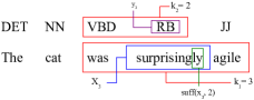
Figure 2: Example of features for a POS task.

Then, at position $s=3$, the following features $h_{1}\in{\mathcal{H}}_{3}^{\text{w}}(3)$, $h_{2}\in{\mathcal{H}}_{2}^{\text{tag}}(3)$, $h_{3}\in{\mathcal{H}}_{1}^{\text{sp}}(3)$ would activate:

$$h_{1}(x)=\mathbf{1}_{x_{2}=\text{`was'},\,x_{3}=\text{`surprisingly'},\,x_{4}=\text{`agile'}}(x)$$

$$h_{2}(y)=\mathbf{1}_{y_{2}=\text{'VBD'},\,y_{3}=\text{`RB'}}(y)$$

$$h_{3}(x)=\mathbf{1}_{\text{suff}(x_{3},2)=\text{`ly'}}(x).$$

See Figure 2 for an illustration.

Now, recall that the VCRF algorithm requires knowledge of complexities $r(H_{k_{1},k_{2},k_{3}})$. By definition of the hypothesis set and $r_{k}$s

$$r(H_{k_{1},k_{2},k_{3}})\leq\sqrt{\frac{2(k_{1}\log|V|+k_{2}\log|\Delta|+k_{3}\log|\Sigma|}{m}},$$ (18)

which is precisely the complexity penalty used in our experiments.

The impact of this added penalization can be seen in Table 3, where it is seen that the number of non-zero features for VCRF can be dramatically smaller than the number for $L_{1}$-regularized CRF.

B.3 Hyperparameter tuning and cross-validation

Recall that the VCRF algorithm admits two hyperparameters $\lambda$ and $\beta$. In our experiments, we optimized over $\lambda,\beta\in\{1,0.5,10^{-1},\ldots,10^{-5},0\}$. We compared VCRF against $L_{1}$-regularized CRF, which is the special case of VCRF with $\lambda=0$. For gradient computation, we used the procedure in Section D.2.1, which is agnostic to the choice of the underlying loss function. While our algorithms can be used with very general families of loss functions this choice allows an easy direct comparison with the CRF algorithm. We ran each algorithm for 50 full passes over the entire training set or until convergence.

Table 2: Experimental results for both VCRF and CRF. VCRF refers to the conditional random field objective with both VRM-style regularization and $L_{1}$ regularization while CRF refers to the objective with only $L_{1}$ regularization. Boldfaced results are statistically significant at a 5% confidence level.

	VCRF error (%)		CRF error(%)
Dataset	Token	Sentence	Token	Sentence
Basque	7.26 $\pm$ 0.13	57.67 $\pm$ 0.82	17.68 $\pm$ 0.20	59.78 $\pm$ 1.39
Chinese	7.38 $\pm$ 0.15	67.73 $\pm$ 0.46	17.67 $\pm$ 0.12	68.88 $\pm$ 0.49
Dutch	5.97 $\pm$ 0.08	49.27 $\pm$ 0.71	16.01 $\pm$ 0.92	49.48 $\pm$ 1.02
English	5.51 $\pm$ 0.04	44.40 $\pm$ 1.30	15.51 $\pm$ 0.06	44.32 $\pm$ 1.31
Finnish	7.48 $\pm$ 0.05	55.96 $\pm$ 0.64	17.86 $\pm$ 0.13	57.17 $\pm$ 1.36
Finnish-FTB	9.79 $\pm$ 0.22	51.23 $\pm$ 1.21	10.55 $\pm$ 0.22	52.98 $\pm$ 0.75
Hindi	4.84 $\pm$ 0.10	51.69 $\pm$ 1.07	14.93 $\pm$ 0.08	53.18 $\pm$ 0.75
Tamil	19.82 $\pm$ 0.69	89.83 $\pm$ 2.13	22.50 $\pm$ 1.57	92.00 $\pm$ 1.54
Turkish	11.28 $\pm$ 0.40	59.63 $\pm$ 1.55	11.69 $\pm$ 0.37	61.15 $\pm$ 1.01
Twitter	17.98 $\pm$ 1.25	75.57 $\pm$ 1.25	19.81 $\pm$ 1.09	76.96 $\pm$ 1.37

In each of the experiments, we used 5-fold cross-validation for model selection and performance evaluation. Each dataset was randomly partitioned into $5$ folds, and each algorithm was run $5$ times, with a different assignment of folds to the training set, validation set and test set for each run. For each run $i\in\{0,\ldots,4\}$, fold $i$ was used for validation, fold $i+1(\text{ mod }5)$ was used for testing, and the remaining folds were used for training. In each run, we selected the parameters that had the lowest token error on the validation set and then measured the token and sentence error of those parameters on the test set. The average error and the standard deviation of the errors are reported in Table 2 for each data set.

B.4 More experiments

In this section, we present our results for a POS tagging task when noise is artificially injected into the labels. Specifically, for tokens corresponding to features that commonly appear in the dataset (at least five times in our experiments), we flip their associated POS label to some other arbitrary label with 20% probability.

The results of these experiments are given in Table 4. They demonstrate that VCRF outperforms $L_{1}$-CRF in the majority of cases. Moreover, these differences can be magnified from the original scenario, as can be seen on the English and Twitter datasets.

Table 3: Average number of features for VCRF and $L_{1}$-CRF.

Dataset	VCRF	CRF	Ratio
Basque	7028	94712653	0.00007
Chinese	219736	552918817	0.00040
Dutch	2646231	2646231	1.00000
English	4378177	357011992	0.01226
Finnish	32316	89333413	0.00036
Finnish-FTB	53337	5735210	0.00930
Hindi	108800	448714379	0.00024
Tamil	1583	668545	0.00237
Turkish	498796	3314941	0.15047
Twitter	18371	26660216	0.000689

Table 4: Experimental results of both VCRF and CRF with 20% random noise added to the training set. Labels of tokens are flipped uniformly at random with 20% probability. Boldfaced results are statistically significant at a 5% confidence level.

	VCRF error (%)		CRF error(%)
Dataset	Token	Sentence	Token	Sentence
Basque	9.13 $\pm$ 0.18	67.43 $\pm$ 0.93	9.42 $\pm$ 0.31	68.61 $\pm$ 1.08
Chinese	96.43 $\pm$ 0.33	100.00 $\pm$ 0.01	96.81 $\pm$ 0.43	100.00 $\pm$ 0.01
Dutch	8.16 $\pm$ 0.52	62.15 $\pm$ 1.77	8.57 $\pm$ 0.30	63.55 $\pm$ 0.87
English	8.79 $\pm$ 0.23	61.27 $\pm$ 1.21	9.20 $\pm$ 0.11	63.60 $\pm$ 1.18
Finnish	9.38 $\pm$ 0.27	64.96 $\pm$ 0.89	9.62 $\pm$ 0.18	65.91 $\pm$ 0.93
Finnish-FTB	11.39 $\pm$ 0.29	72.56 $\pm$ 1.30	11.76 $\pm$ 0.25	73.63 $\pm$ 1.19
Hindi	6.63 $\pm$ 0.51	63.84 $\pm$ 2.86	7.85 $\pm$ 0.33	71.93 $\pm$ 1.20
Tamil	20.77 $\pm$ 0.70	93.00 $\pm$ 1.35	21.36 $\pm$ 0.86	93.50 $\pm$ 1.78
Turkish	14.28 $\pm$ 0.46	69.72 $\pm$ 1.51	14.31 $\pm$ 0.53	69.62 $\pm$ 2.04
Twitter	90.92 $\pm$ 1.67	100.00 $\pm$ 0.00	92.27 $\pm$ 0.71	100.00 $\pm$ 0.00

Appendix C Voted Structured Boosting (VStructBoost)

In this section, we consider algorithms based on the StructBoost surrogate loss, where we choose $\Phi_{u}(v)=ue^{-v}$. Let $\delta{\mathbf{\Psi}}(x,y,y^{\prime})={\mathbf{\Psi}}(x,y)-{\mathbf{\Psi}}(x,y^{\prime})$. This then leads to the following optimization problem:

$$\min_{{\mathbf{w}}}\frac{1}{m}\sum_{i=1}^{m}\max_{y\neq y_{i}}{\mathsf{L}}(y,y_{i})e^{-{\mathbf{w}}\cdot\delta{\mathbf{\Psi}}(x_{i},y_{i},y)}+\sum_{k=1}^{p}(\lambda r_{k}+\beta)\|{\mathbf{w}}_{k}\|_{1}.$$ (19)

One disadvantage of this formulation is that the first term of the objective is not differentiable. Upper bounding the maximum by a sum leads to the following optimization problem:

$$\min_{{\mathbf{w}}}\frac{1}{m}\sum_{i=1}^{m}\sum_{y\neq y_{i}}{\mathsf{L}}(y,y_{i})e^{-{\mathbf{w}}\cdot\delta{\mathbf{\Psi}}(x_{i},y_{i},y)}+\sum_{k=1}^{p}(\lambda r_{k}+\beta)\|{\mathbf{w}}_{k}\|_{1}.$$ (20)

We refer to the learning algorithm based on the optimization problem (20) as VStructBoost. To the best of our knowledge, the formulations (19) and (20) are new, even with the standard $L_{1}$- or $L_{2}$-regularization.

Appendix D Optimization solutions

Here, we show how the optimization problems in (10) and (20) can be solved efficiently when the feature vectors admit a particular factor graph decomposition that we refer to as Markov property.

D.1 Markovian features

We will consider in what follows the common case where ${\mathcal{Y}}$ is a set of sequences of length $l$ over a finite alphabet $\Delta$ of size $r$. Other structured problems can be treated in similar ways. We will denote by $\varepsilon$ the empty string and for any sequence $y=(y_{1},\ldots,y_{l})\in{\mathcal{Y}}$, we will denote by $y_{s}^{s^{\prime}}=(y_{s},\ldots,y_{s^{\prime}})$ the substring of $y$ starting at index $s$ and ending at $s^{\prime}$. For convenience, for $s\leq 0$, we define $y_{s}$ by $y_{s}=\varepsilon$.

One common assumption that we shall adopt here is that the feature vector ${\mathbf{\Psi}}$ admits a Markovian property of order $q$. By this, we mean that it can be decomposed as follows for any $(x,y)\in{\mathcal{X}}\times{\mathcal{Y}}$:

$${\mathbf{\Psi}}(x,y)=\sum_{s=1}^{l}{\boldsymbol{\psi}}(x,y_{s-q+1}^{s},s).$$ (21)

for some position-dependent feature vector function ${\boldsymbol{\psi}}$ defined over ${\mathcal{X}}\times\Delta^{q}\times[l]$. This also suggests a natural decomposition of the family of feature vectors ${\mathbf{\Psi}}=({\mathbf{\Psi}}_{1},\ldots,{\mathbf{\Psi}}_{p})$ for the application of VRM principle where ${\mathbf{\Psi}}_{k}$ is a Markovian feature vector of order $k$. Thus, ${\mathcal{F}}_{k}$ then consists of the family of Markovian feature functions of order $k$. We note that we can write ${\mathbf{\Psi}}=\sum_{k=1}^{p}\tilde{\mathbf{\Psi}}_{k}$ with $\tilde{\mathbf{\Psi}}_{k}=(0,\ldots,{\mathbf{\Psi}}_{k},\ldots,0)$. In the following, abusing the notation, we will simply write ${\mathbf{\Psi}}_{k}$ instead of $\tilde{\mathbf{\Psi}}_{k}$. Thus, for any $x\in{\mathcal{X}}$ and $y\in{\mathcal{Y}}$,

$${\mathbf{\Psi}}({\mathbf{x}},y)=\sum_{k=1}^{p}{\mathbf{\Psi}}_{k}(x,y).$$ (22)

For any $k\in[1,p]$, let ${\boldsymbol{\psi}}_{k}$ denote the position-dependent feature vector function corresponding to ${\mathbf{\Psi}}_{k}$. Also, for any $x\in{\mathcal{X}}$ and $y\in\Delta^{l}$, define $\widetilde{\boldsymbol{\psi}}$ by $\widetilde{\boldsymbol{\psi}}(x,y_{s-p+1}^{s},s)=\sum_{k=1}^{p}{\boldsymbol{\psi}}_{k}(x,y_{s-k+1}^{s},s)$. Observe then that we can write

$${\mathbf{\Psi}}(x,y)=\sum_{k=1}^{p}{\mathbf{\Psi}}_{k}(x,y) =\sum_{k=1}^{p}\sum_{s=1}^{l}{\boldsymbol{\psi}}_{k}(x,y_{s-k+1}^{s},s)$$

$$=\sum_{s=1}^{l}\sum_{k=1}^{p}{\boldsymbol{\psi}}_{k}(x,y_{s-k+1}^{s},s)$$

$$=\sum_{s=1}^{l}\widetilde{\boldsymbol{\psi}}(x_{i},y_{s-p+1}^{s},s).$$ (23)

In Sections D.2 and D.3, we describe algorithms for efficiently computing the gradient by leveraging the underlying graph structure of the problem.

D.2 Efficient gradient computation for VCRF

In this section, we show how Gradient Descent (GD) and Stochastic Gradient Descent (SGD) can be used to solve the optimization problem of VCRF. To do so, we will show how the subgradient of the contribution to the objective function of a given point $x_{i}$ can be computed efficiently. Since the computation of the subgradient of the regularization term presents no difficulty, it suffices to show that the gradient of $F_{i}$, the contribution of point $x_{i}$ to the empirical loss term for an arbitrary $i\in[m]$, can be computed efficiently. In the special case of the Hamming loss or when loss is omitted from the objective altogether, this coincides with the standard CRF training procedure. We extend this to more general families of loss function.

Fix $i\in[m]$. For the VCRF objective, $F_{i}$ can be rewritten as follows:

$$F_{i}({\mathbf{w}})=\frac{1}{m}\log\bigg{(}\sum_{y\in{\mathcal{Y}}}e^{{\mathsf{L}}(y,y_{i})-{\mathbf{w}}\cdot\delta{\mathbf{\Psi}}(x_{i},y_{i},y)}\bigg{)}=\frac{1}{m}\log\bigg{(}\sum_{y\in{\mathcal{Y}}}e^{{\mathsf{L}}(y,y_{i})+{\mathbf{w}}\cdot{\mathbf{\Psi}}(x_{i},y)}\bigg{)}-\frac{{\mathbf{w}}\cdot{\mathbf{\Psi}}(x_{i},y_{i})}{m}.$$

The following lemma gives the expression of the gradient of $F_{i}$ and helps identify the key computationally challenging terms ${\mathsf{q}}_{\mathbf{w}}$.

Lemma 15.

The gradient of $F_{i}$ at any ${\mathbf{w}}$ can be expressed as follows:

$$\nabla F_{i}({\mathbf{w}})=\frac{1}{m}\sum_{s=1}^{l}\sum_{{\mathbf{z}}\in\Delta^{p}}\Bigg{[}\sum_{y\colon y_{s-p+1}^{s}={\mathbf{z}}}{\mathsf{q}}_{\mathbf{w}}(y)\Bigg{]}\widetilde{\boldsymbol{\psi}}(x_{i},{\mathbf{z}},s)-\frac{{\mathbf{\Psi}}(x_{i},y_{i})}{m},$$

where, for all $y\in{\mathcal{Y}}$,

$${\mathsf{q}}_{\mathbf{w}}(y)=\frac{e^{{\mathsf{L}}(y,y_{i})+{\mathbf{w}}\cdot{\mathbf{\Psi}}(x_{i},y)}}{Z_{\mathbf{w}}},$$

$$Z_{\mathbf{w}}=\sum_{y\in{\mathcal{Y}}}e^{{\mathsf{L}}(y,y_{i})+{\mathbf{w}}\cdot{\mathbf{\Psi}}(x_{i},y)}.$$

Proof.

In view of the expression of $F_{i}$ given above, the gradient of $F_{i}$ at any ${\mathbf{w}}$ is given by

$$\nabla F_{i}({\mathbf{w}}) =\frac{1}{m}\sum_{y\in{\mathcal{Y}}}\frac{e^{{\mathsf{L}}(y,y_{i})+{\mathbf{w}}\cdot{\mathbf{\Psi}}(x_{i},y)}}{\sum_{\tilde{y}\in{\mathcal{Y}}}e^{{\mathsf{L}}(\tilde{y},y_{i})+{\mathbf{w}}\cdot{\mathbf{\Psi}}(x_{i},\tilde{y})}}{\mathbf{\Psi}}(x_{i},y)-\frac{{\mathbf{\Psi}}(x_{i},y_{i})}{m}$$

$$=\frac{1}{m}\operatorname*{\mathbb{E}}_{y\sim{\mathsf{q}}_{\mathbf{w}}}[{\mathbf{\Psi}}(x_{i},y)]-\frac{{\mathbf{\Psi}}(x_{i},y_{i})}{m}.$$

By (23), we can write

$$\operatorname*{\mathbb{E}}_{y\sim{\mathsf{q}}_{\mathbf{w}}}[{\mathbf{\Psi}}(x_{i},y)]=\sum_{y\in\Delta^{l}}{\mathsf{q}}_{\mathbf{w}}(y)\sum_{s=1}^{l}\widetilde{\boldsymbol{\psi}}(x_{i},y_{s-p+1}^{s},s)=\sum_{s=1}^{l}\sum_{{\mathbf{z}}\in\Delta^{p}}\Bigg{[}\sum_{y\colon y_{s-p+1}^{s}={\mathbf{z}}}{\mathsf{q}}_{\mathbf{w}}(y)\Bigg{]}\widetilde{\boldsymbol{\psi}}(x_{i},{\mathbf{z}},s),$$

which completes the proof. ∎

The lemma implies that the key computation in the gradient is

$${\mathsf{Q}}_{\mathbf{w}}({\mathbf{z}},s)=\sum_{y\colon y_{s-p+1}^{s}={\mathbf{z}}}{\mathsf{q}}_{\mathbf{w}}(y)=\sum_{y\colon y_{s-p+1}^{s}={\mathbf{z}}}\frac{e^{{\mathsf{L}}(y,y_{i})}\,\prod_{t=1}^{l}e^{{\mathbf{w}}\cdot\widetilde{\boldsymbol{\psi}}(x_{i},y_{t-p+1}^{t},t)}}{Z_{\mathbf{w}}},$$ (24)

for all $s\in[l]$ and ${\mathbf{z}}\in\Delta^{p}$. The sum defining these terms is over a number of sequences $y$ that is exponential in $|\Delta|$. However, we will show in the following sections how to efficiently compute ${\mathsf{Q}}_{\mathbf{w}}({\mathbf{z}},s)$ for any $s\in[l]$ and ${\mathbf{z}}\in\Delta^{p}$ in several important cases: (0) in the absence of a loss; (1) when ${\mathsf{L}}$ is Markovian; (2) when ${\mathsf{L}}$ is a rational loss; and (3) when ${\mathsf{L}}$ is the edit-distance or any other tropical loss.

D.2.1 Gradient computation in the absence of a loss

In that case, it suffices to show how to compute $Z^{\prime}_{\mathbf{w}}=\sum_{y\in{\mathcal{Y}}}e^{{\mathbf{w}}\cdot{\mathbf{\Psi}}(x_{i},y)}$ and the following term, ignoring the loss factors:

$${\mathsf{Q}}^{\prime}_{\mathbf{w}}({\mathbf{z}},s)=\sum_{y\colon y_{s-p+1}^{s}={\mathbf{z}}}\prod_{t=1}^{l}e^{{\mathbf{w}}\cdot\widetilde{\boldsymbol{\psi}}(x_{i},y_{t-p+1}^{t},t)},$$ (25)

for all $s\in[l]$ and ${\mathbf{z}}\in\Delta^{p}$. We will show that ${\mathsf{Q}}^{\prime}_{\mathbf{w}}({\mathbf{z}},s)$ coincides with the flow through an edge of a weighted graph we will define, which leads to an efficient computation. We will use for any $y\in\Delta^{l}$, the convention $y_{s}=\varepsilon$ if $s\leq 0$. Now, let ${\mathscr{A}}$ be the weighted finite automaton (WFA) with the following set of states:

$$Q_{\mathscr{A}}=\Big{\{}(y_{t-p+1}^{t},t)\colon y\in\Delta^{l},t=0,\ldots,l\Big{\}},$$

with $I_{\mathscr{A}}=(\varepsilon,0)$ its single initial state, $F_{\mathscr{A}}=\{(y_{l-p+1}^{l},l)\colon y\in\Delta^{l}\}$ its set of final states, and a transition from state $(y_{t-p+1}^{t-1},t-1)$ to state $(y_{t-p+2}^{t-1}\,b,t)$ with label $b$ and weight $\omega(y_{t-p+1}^{t-1}\,b,t)=e^{{\mathbf{w}}\cdot\widetilde{\boldsymbol{\psi}}(x_{i},y_{t-p+1}^{t-1}b,t)}$, that is the following set of transitions:

$$E_{\mathscr{A}}=\Big{\{} \Big{(}(y_{t-p+1}^{t-1},t-1),b,\omega(y_{t-p+1}^{t-1}\,b,t),(y_{t-p+2}^{t-1}\,b,t)\Big{)}\colon y\in\Delta^{l},b\in\Delta,t\in[l]\Big{\}}.$$

Figure 3 illustrates this construction in the case $p=2$. The WFA ${\mathscr{A}}$ is deterministic by construction. The weight of a path in ${\mathscr{A}}$ is obtained by multiplying the weights of its constituent transitions. In view of that, ${\mathsf{Q}}^{\prime}_{\mathbf{w}}({\mathbf{z}},s)$ can be seen as the sum of the weights of all paths in ${\mathscr{A}}$ going through the transition from state $({\mathbf{z}}_{1}^{p-1},s-1)$ to $({\mathbf{z}}_{2}^{p},s)$ with label $z_{p}$.

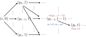
Figure 3: Illustration of WFA ${\mathscr{A}}$ for $p=2$.

For any state $(y_{t-p+1}^{t},t)\in Q_{\mathscr{A}}$, let $\alpha((y_{t-p+1}^{t},t))$ denote the sum of the weights of all paths in ${\mathscr{A}}$ from $I_{\mathscr{A}}$ to $(y_{t-p+1}^{t},t)$ and $\beta((y_{t-p+1}^{t},t))$ the sum of the weights of all paths from $(y_{t-p+1}^{t},t)$ to a final state. Then, ${\mathsf{Q}}^{\prime}_{\mathbf{w}}({\mathbf{z}},s)$ is given by

$${\mathsf{Q}}^{\prime}_{\mathbf{w}}({\mathbf{z}},s)=\alpha\big{(}({\mathbf{z}}_{1}^{p-1},s-1)\big{)}\times\omega({\mathbf{z}},s)\times\beta\big{(}({\mathbf{z}}_{2}^{p},s)\big{)}.$$

Note also that $Z^{\prime}_{\mathbf{w}}$ is simply the sum of the weights of all paths in ${\mathscr{A}}$, that is $Z^{\prime}_{\mathbf{w}}=\beta((\varepsilon,0))$.

Since ${\mathscr{A}}$ is acyclic, $\alpha$ and $\beta$ can be computed for all states in linear time in the size of ${\mathscr{A}}$ using a single-source shortest-distance algorithm over the $(+,\times)$ semiring or the so-called forward-backward algorithm. Thus, since ${\mathscr{A}}$ admits $O(l|\Delta|^{p})$ transitions, we can compute all of the quantities ${\mathsf{Q}}^{\prime}_{\mathbf{w}}({\mathbf{z}},s)$, $s\in[l]$ and $z\in\Delta^{p}$ and $Z^{\prime}_{\mathbf{w}}$, in time $O(l|\Delta|^{p})$.

D.2.2 Gradient computation with a Markovian loss

We will say that a loss function ${\mathsf{L}}$ is Markovian if it admits a decomposition similar to the features, that is for all $y,y^{\prime}\in{\mathcal{Y}}$,

$${\mathsf{L}}(y,y^{\prime})=\sum_{t=1}^{l}{\mathsf{L}}_{t}(y_{t-p+1}^{t},{y^{\prime}}_{t-p+1}^{t}).$$

In that case, we can absorb the losses in the transition weights and define new transition weights $\omega^{\prime}$ as follows:

$$\omega^{\prime}(t,y_{t-p+1}^{t-1}\,b)=e^{L_{t}(y_{t-p+1}^{t-1}\,b,{(y_{i})}_{t-p+1}^{t-1}\,b)}\omega(y_{t-p+1}^{t-1}\,b,t).$$

Using the resulting WFA ${\mathscr{A}}^{\prime}$ and precisely the same techniques as those described in the previous section, we can compute all ${\mathsf{Q}}_{\mathbf{w}}({\mathbf{z}},s)$ in time $O(l|\Delta|^{p})$. In particular, we can compute efficiently these quantities in the case of the Hamming loss which is a Markovian loss for $p=1$.

D.3 Efficient gradient computation for VStructBoost

In this section, we briefly describe the gradient computation for VStructBoost, which follows along similar lines as the discussion for VCRF.

Fix $i\in[m]$ and let $F_{i}$ denote the contribution of point $x_{i}$ to the empirical loss in VStructBoost. Using the equality ${\mathsf{L}}(y_{i},y_{i})=0$, $F_{i}$ can be rewritten as

$$F_{i}({\mathbf{w}}) =\frac{1}{m}\sum_{y\neq y_{i}}{\mathsf{L}}(y,y_{i})e^{-{\mathbf{w}}\cdot\delta{\mathbf{\Psi}}(x_{i},y_{i},y)}=\frac{1}{m}e^{-{\mathbf{w}}\cdot{\mathbf{\Psi}}(x_{i},y_{i})}\sum_{y\in\Delta^{l}}{\mathsf{L}}(y,y_{i})e^{{\mathbf{w}}\cdot{\mathbf{\Psi}}(x_{i},y)}.$$

The gradient of $F_{i}$ can therefore be expressed as follows:

$$\nabla F_{i}({\mathbf{w}}) =\frac{1}{m}e^{-{\mathbf{w}}\cdot{\mathbf{\Psi}}(x_{i},y_{i})}\sum_{y\in\Delta^{l}}{\mathsf{L}}(y,y_{i})e^{{\mathbf{w}}\cdot{\mathbf{\Psi}}(x_{i},y)}{\mathbf{\Psi}}(x_{i},y)$$ (26)

$$\quad-\frac{1}{m}e^{-{\mathbf{w}}\cdot{\mathbf{\Psi}}(x_{i},y_{i})}{\mathbf{\Psi}}(x_{i},y_{i})\sum_{y\in\Delta^{l}}{\mathsf{L}}(y,y_{i})e^{{\mathbf{w}}\cdot{\mathbf{\Psi}}(x_{i},y)}.$$

Efficient computation of these terms is not straightforward, since the sums run over exponentially many sequences $y$. However, by leveraging the Markovian property of the features, we can reduce the calculation to flow computations over a weighted directed graph, in a manner analogous to what we demonstrated for VCRF.

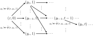
Figure 4: Illustration of the WFA ${\mathscr{A}}^{\prime}$ for $p=2$.

D.4 Inference

In this section, we describe an efficient algorithm for inference when using Markovian features. The algorithm consists of a standard single-source shortest-path algorithm applied to a WFA ${\mathscr{A}}^{\prime}$ differs from the WFA ${\mathscr{A}}$ only by the weight of each transition, defined as follows:

$$E_{{\mathscr{A}}^{\prime}}=\Big{\{}\Big{(} (\bar{y}_{t-p+1}^{t-1},t-1),b,{\mathbf{w}}\cdot\widetilde{\boldsymbol{\psi}}(x,y_{t-p+1}^{t-1}b,t),(\bar{y}_{t-p+2}^{t-1}\,b,t)\Big{)}\colon y\in\Delta^{l},b\in\Delta,t\in[l]\Big{\}}.$$

Furthermore, here, the weight of a path is obtained by adding the weights of its constituent transitions. Figure 4 shows ${\mathscr{A}}^{\prime}$ in the special case of $p=2$. By construction, the weight of the unique accepting path in ${\mathscr{A}}^{\prime}$ labeled with $y\in\Delta^{l}$ is $\sum_{t=1}^{l}{\mathbf{w}}\cdot\widetilde{\boldsymbol{\psi}}(x,y_{t-p+1}^{t-1}b,t)={\mathbf{w}}\cdot{\mathbf{\Psi}}(x,y)$.

Thus, the label of the single-source shortest path, $\operatorname*{argmin}_{y\in\Delta^{l}}{\mathbf{w}}\cdot{\mathbf{\Psi}}(x,y)$, is the desired predicted label. Since ${\mathscr{A}}^{\prime}$ is acyclic, the running-time complexity of the algorithm is linear in the size of ${\mathscr{A}}^{\prime}$, that is $O(l|\Delta|^{l})$.

References

- Bakir et al. [2007] G. H. Bakir, T. Hofmann, B. Schölkopf, A. J. Smola, B. Taskar, and S. V. N. Vishwanathan. Predicting Structured Data (Neural Information Processing). The MIT Press, 2007.
- Chang et al. [2015] K. Chang, A. Krishnamurthy, A. Agarwal, H. Daumé III, and J. Langford. Learning to search better than your teacher. In ICML, 2015.
- Collins [2001] M. Collins. Parameter estimation for statistical parsing models: Theory and practice of distribution-free methods. In Proceedings of IWPT, 2001.
- Cortes et al. [2007] C. Cortes, M. Mohri, and J. Weston. A General Regression Framework for Learning String-to-String Mappings. In Predicting Structured Data. MIT Press, 2007.
- Cortes et al. [2014] C. Cortes, V. Kuznetsov, and M. Mohri. Ensemble methods for structured prediction. In ICML, 2014.
- Cortes et al. [2015] C. Cortes, P. Goyal, V. Kuznetsov, and M. Mohri. Kernel extraction via voted risk minimization. JMLR, 2015.
- Daumé III et al. [2009] H. Daumé III, J. Langford, and D. Marcu. Search-based structured prediction. Machine Learning, 75(3):297–325, 2009.
- Doppa et al. [2014] J. R. Doppa, A. Fern, and P. Tadepalli. Structured prediction via output space search. JMLR, 15(1):1317–1350, 2014.
- Jurafsky and Martin [2009] D. Jurafsky and J. H. Martin. Speech and Language Processing (2nd Edition). Prentice-Hall, Inc., 2009.
- Kuznetsov et al. [2014] V. Kuznetsov, M. Mohri, and U. Syed. Multi-class deep boosting. In NIPS, 2014.
- Lafferty et al. [2001] J. Lafferty, A. McCallum, and F. Pereira. Conditional random fields: Probabilistic models for segmenting and labeling sequence data. In ICML, 2001.
- Lam et al. [2015] M. Lam, J. R. Doppa, S. Todorovic, and T. G. Dietterich. c-search for structured prediction in computer vision. In CVPR, 2015.
- Lei et al. [2015] Y. Lei, Ü. D. Dogan, A. Binder, and M. Kloft. Multi-class svms: From tighter data-dependent generalization bounds to novel algorithms. In NIPS, 2015.
- Lucchi et al. [2013] A. Lucchi, L. Yunpeng, and P. Fua. Learning for structured prediction using approximate subgradient descent with working sets. In CVPR, 2013.
- Maurer [2016] A. Maurer. A vector-contraction inequality for rademacher complexities. In ALT, 2016.
- McAllester [2007] D. McAllester. Generalization bounds and consistency for structured labeling. In Predicting Structured Data. MIT Press, 2007.
- Mohri et al. [2012] M. Mohri, A. Rostamizadeh, and A. Talwalkar. Foundations of Machine Learning. The MIT Press, 2012.
- Nadeau and Sekine [2007] D. Nadeau and S. Sekine. A survey of named entity recognition and classification. Linguisticae Investigationes, 30(1):3–26, January 2007.
- Ross et al. [2011] S. Ross, G. J. Gordon, and D. Bagnell. A reduction of imitation learning and structured prediction to no-regret online learning. In AISTATS, 2011.
- Taskar et al. [2003] B. Taskar, C. Guestrin, and D. Koller. Max-margin Markov networks. In NIPS, 2003.
- Tsochantaridis et al. [2005] I. Tsochantaridis, T. Joachims, T. Hofmann, and Y. Altun. Large margin methods for structured and interdependent output variables. JMLR, 6:1453–1484, Dec. 2005.
- Vinyals et al. [2015a] O. Vinyals, L. Kaiser, T. Koo, S. Petrov, I. Sutskever, and G. Hinton. Grammar as a foreign language. In NIPS, 2015a.
- Vinyals et al. [2015b] O. Vinyals, A. Toshev, S. Bengio, and D. Erhan. Show and tell: A neural image caption generator. In CVPR, 2015b.
- Zhang et al. [2008] D. Zhang, L. Sun, and W. Li. A structured prediction approach for statistical machine translation. In IJCNLP, 2008.