Universality of (2+1)-dimensional restricted solid-on-solid models
Abstract
Extensive dynamical simulations of restricted solid on solid models in dimensions have been done using parallel multisurface algorithms implemented on graphics cards. Numerical evidence is presented that these models exhibit Kardar–Parisi–Zhang surface growth scaling, irrespective of the step heights . We show that by increasing the corrections to scaling increase, thus smaller step sized models describe better the asymptotic, long-wave-scaling behavior.
pacs:
05.70.Ln, 05.70.Np, 82.20.WtI Introduction
The Kardar–Parisi–Zhang (KPZ) equation Kardar et al. (1986) describes the evolution of a fundamental, non-equilibrium surface growth model by a Langevin equation
| (1) |
The scalar field is the height, progressing in the dimensional space relative to its mean position, that moves linearly with time . A smoothing surface tension is represented by the coefficient , which competes a curvature-driven propagation, described by the nonlinear coefficient and a zero-average Gaussian stochastic noise. This noise field exhibits the variance , with an amplitude, related to the temperature in the equilibrium system, and denotes a distribution average. Besides describing the dynamics of simple growth processes Halpin-Healy (1990) KPZ was inspired in part by the stochastic Burgers equation Burgers (1974) and is applicable for randomly stirred fluids Forster et al. (1977), for directed polymers in random media Kardar (1985) for dissipative transport van Beijeren et al. (1985); Janssen and Schmittmann (1986) and for the magnetic flux lines in superconductors Hwa (1992).
Discretized versions have been studied frequently over the past few decades Meakin et al. (1986); Barabási and Stanley (1995); Krug (1997). The morphology of a surface of linear size can be described by the squared interface width
| (2) |
In the absence of any characteristic length simple growth processes are expected to be scale-invariant
| (3) |
with the universal scaling function
| (4) |
Here is the roughness exponent in the stationary regime, when the correlation length has exceeded and is the growth exponent, describing the intermediate time behavior. The dynamical exponent can be expressed as the ratio of the growth exponents
| (5) |
and due to the Galilean invariance the relation holds as well.
While in exact solutions are known, due to the Galilean symmetry Forster et al. (1977) and an incidental fluctuation-dissipation symmetry Kardar (1987), in higher dimensions KPZ has been investigated by various analytical Kloss et al. (2012); Schwartz and Edwards (1992); Frey and Täuber (1994); Lässig (1995); Fogedby (2005); Canet et al. (2011) and numerical methods Forrest and Tang (1990); Halpin-Healy (2012); Marinari et al. (2000); Aarão Reis (2005), still debated issues remain. For example, there is a controversy on the surface growth exponents of the KPZ, obtained by recent simulations Kelling and Ódor (2011); Alves et al. (2014a) and a field theoretical study Lässig (1998). Assuming that the height correlations do not exhibit multi-scaling and satisfy an operator product expansion Ref. Lässig (1998) concluded that growth exponents are rational numbers in two and three dimensions Lässig (1998). This was in accordance with some earlier restricted solid-on-solid (RSOS) model simulation results Kim and Kosterlitz (1989); Kim et al. (1991). Recent high precision simulations Halpin-Healy (2013); Alves et al. (2014b); Kelling and Ódor (2011); Alves et al. (2014a); Pagnani and Parisi (2015) all excluded this and concluded Kelling and Ódor (2011); Pagnani and Parisi (2015); Alves et al. (2014a) and Kelling and Ódor (2011). RSOS models are defined by deposition at random sites if the local height difference satisfies
| (6) |
Very recently Kim Kim (2015) investigated RSOS models with maximum step sizes . As he increased the roughness exponent seemed to converge to and the growth exponent to in agreement with Kim and Kosterlitz (1989); Kim et al. (1991); Lässig (1998). This issue is important, because one may speculate that discretized simulations cannot describe the local singularities of continuum models, i.e. finite slopes may cause corrections, responsible for the longstanding debate between field theory and discrete model simulations.
In this paper we show that the converse is true. By performing very careful corrections-to-scaling analysis on the model of Ref. Kim et al. (1991); Kim (2015) we show that even in case of the rational numbers of Kim and Kosterlitz (1989); Kim et al. (1991); Lässig (1998) can be excluded in the limit. Local slopes analysis shows, that the case has the smallest corrections and describes the KPZ universality scaling the best. For corrections corresponding shorter wavelengths are introduced. Our findings are in full agreement with the scaling results obtained for ballistic growth models Alves et al. (2014a); Alves and Ferreira (2016); Alves .
II Models and simulation algorithms
In order to enable long time surface growth simulations of large systems, a multisurface-like parallel implementation of the RSOS model has been created for graphics processing units (GPUs). Two parallelization approaches have been combined as follows:
Since GPUs feature a number of vector processors, multiples of realizations of the model were simulated simultaneously. This creates a data-parallel workload, which can straightforwardly be vectorized. Each single instruction multiple thread (SIMT) unit of the GPU updates realizations, in which the sequence of randomly selected coordinates for update is the same. This correlation was broken by updating only half of the selected lattice sites in each attempt. If more realizations were simulated, different sets of realizations evolved completely independently.
In order to handle large systems effectively a domain decomposition (DD) was also used to distribute the work of realizations among multiple SIMT elements. A double-tiling scheme was applied by splitting up the simulation cells into tiles, split further into two sub-tiles along each spatial direction Kelling et al. (2012). In the present two-dimensional problem this yields sets of sub-tiles, each of which can be updated by multiple independent workers. After each lattice sweep the origin of the DD was moved randomly to eliminate correlations. Implementation details will be published elsewhere Kelling et al. (2016).
Roughening of -dimensional RSOS surfaces was studied for restriction parameters , by starting from flat initial conditions. To obtain estimates for the exponent , the growth of surfaces was followed up to Monte-Carlo steps (MCS), which is well before the correlation length approaches the system sizes: , and studied here (throughout this paper the time is measured in MCS). The largest system size was bounded by memory constraints, filling up \SI12GB of the NVIDIA K40 GPU, and leaving some memory for the random number generator (RNG) states. The results were averaged over and realizations, respectively, where the latter two correspond to only one multisurface run.
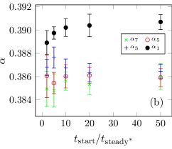
The exponent was determined by a finite-size scaling analysis of the saturation roughness of system sizes between and . To keep the noise amplitude constant we used domain sizes of lattice sites. We determined the interface width by averaging over for times and for all samples. We checked whether the averaged values belong to the steady state: by varying , the onset times of the measurements. We estimated via the relation
| (7) |
using the parameters and , deduced from fitting in small systems.
In order to estimate the asymptotic values of and for and , respectively, a local slopes analysis of the scaling laws was performed Ódor (2008). We calculated the effective exponents
| (8) | ||||
| (9) |
In our studies the simulation time between two measurements is increased exponentially
| (10) |
using and , while statistical uncertainties are provided as –standard errors, defined as .
III Surface growth results
III.1 The growth regime
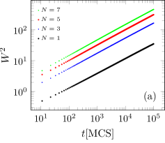
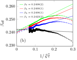
The growth of the surface roughness follows apparently the same, clear, power law (PL) for all considered (Fig. 1(a)). The local slopes plots (Fig. 1(b)), using (9), show an effective growth exponent for for (), in agreement with Kim’s results Kim (2015). Later, the effective growth exponent decreases for all , followed over two orders of magnitude in time in Fig. 1.
Expecting independence of from , it follows that the asymptotic estimates should be the same. By assuming PL corrections to the asymptotic scaling , we obtained a minimal variance of the estimates in case of . Therefore, we plotted our results on the scales, which makes the tails of the curves straight in the limit. Logarithmic corrections to scaling were also tested, but they did not improve the extrapolations.
Table 1 lists the obtained estimates for for the considered system sizes. Results for different are practically identical and are thus averaged to give a common value. The case is listed separately, due to the different corrections to scaling. For , can be best extrapolated by a PL fit with . This is in good agreement with the results of Oliveira et al. (2013), where is reported, based on the KPZ ansatz hypothesis. This motivated us testing more general scaling forms, with correction exponents multiple of . When we combined the effective exponent forms of and ,
| (11) |
with free parameters , fitting for resulted in good agreement for most of the growth region. This is shown for by the dashed lines in Fig. 1(b). From these extrapolations we obtained the estimates: and .
As we can observe in Fig. 1, the effective exponents suffer from stronger corrections for , than in the case. Furthermore, our data suggest a possible oscillating convergence of for , as reported in simulations of the ballistic deposition model (BD) Alves et al. (2014a). Extrapolations based on the form (11), while in good agreement within the observed region, are prone to over-fitting, where they can not cover all possible corrections. The values for are thus underestimated, if the effective exponents do indeed show oscillating convergence.
The estimates show no clear dependence on system size, thus it can be safely assumed that all simulations are well within the scaling regime and do not suffer from finite-size effects. All results are within the margin of error of the octahedron model Kelling and Ódor (2011). Most notably this is also the case for the estimates for . Statistical error measures for single extrapolations do not account for systematic contributions such as from the choice of the extrapolation form or the interval used for a fit. This can be clearly seen by the fact, that many extrapolated values listed above do not agree with each other within such a margin. The spread of these different estimates itself provides a more useful estimate of the margin of error. Overall, the presented data support .
Since the curves in Fig. 1 correspond to the same and sample size , one can observe that the signal-to-noise ratio (S/N), the ratio between the interface width and the sample variance, increases with . For this is higher by a factor of , while for the S/N is about bigger than that of the result. Presumably, the decrease of relative noise level is the consequence of a kind of self-averaging, since systems with larger allowed accommodate more surface information than smaller ones. It is tempting to exploit this property by choosing larger height differences in the simulations, even if this can be implemented less efficiently.
| 4096 | 8192 | 9605 | |
|---|---|---|---|
| 0.2412(1) | 0.2418(1) | 0.2415(1) | |
| 0.2404(3) | 0.2405(3) | 0.2410(3) |
III.2 The steady state
Direct fitting of the finite size scaling form
| (12) |
for and yields the following estimates
For comparison, Kim’s results Kim (2015) are shown in the second column. When we decrease our values decrease slightly but fall inside the error margins if . So, direct fits match perfectly those of Kim (2015), obtained by sequential Monte Carlo updates.
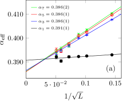
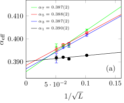
However, if the data are excluded, our estimates become significantly lower, warning for strong corrections to scaling. This can also be seen with the help of the effective exponents in Fig. 2 calculated by (8). There is a clear tendency for to decrease as we increase the system size for the cases. The approach to is nonlinear, but the number of points is insufficient for PL extrapolations to produce consistent estimates. We plotted the results on the scale, resulting in points that can be settled on straight lines. Linear extrapolation to asymptotically large sizes yields:
Corrections to finite-size scaling (12) in case of are small, explaining the good agreement between local slopes analysis and the direct fit. The slight difference between the results for and may be attributed to the fact that our data points are not from deep enough in the steady state. This might also explain the disagreement with the results of a recent study Pagnani and Parisi (2015), which reported for . There is a further uncertainty of the extrapolation to , which is not accounted for by the fit errors. With the assumption of an intrinsic width: Alves and Ferreira (2016), the local slopes analysis shows stronger corrections to scaling, therefore we did not apply this in our study.
The observation of stronger corrections for larger s is consistent with a recent analysis of the BD. Alves et al. (2014a) This study found that corrections to scaling, for both and , are reduced, when the BD surface is smoothened by binning of the surface positions before analysis, thereby decreasing the height differences between neighboring sites. Binning of the surface did not change the universal behavior; it only decreased non-universal corrections. The corrections produced even an oscillatory approach to the asymptotic values of the exponents. This can explain why our simple extrapolations of (Fig. 2) and (Fig. 1) for undershoot those of .
All of our estimates up to , obtained by the local slopes analysis, are in the range , which clearly excludes . Plugging our and results into the scaling relation (5) we get the dynamical exponent estimates and , respectively. The scaling law following from the Galilean invariance is satisfied with these exponents both for : and : within error margins.
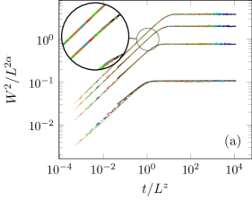
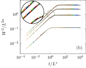
We have also tested the scaling form (3) numerically by using our and values. As Fig. 3 shows, good data collapses can be obtained for and even a perfectly looking one for . For in the growth regime a perfect one can also be achieved assuming the values suggested by Kim and Kosterlitz Kim and Kosterlitz (1989) (Fig. 3(a)). This can be understood by taking into account the corrections to scaling we explored above. Effective exponents for early times and small systems agree with the conjecture by Kim and Kosterlitz (1989) and indeed the most strongly outlying curves in Fig. 3(a), correspond to smaller systems.
Moments of the width and height distributions are defined as:
| (13) | ||||
| where denotes the probability distribution corresponding to the interface observable . We calculated some standard measures of the shape, the skewness | ||||
| (14) | ||||
| and the kurtosis | ||||
| (15) | ||||
in the steady state. These measures were shown to be universal in KPZ models Marinari et al. (2002); Foltin et al. (1994).
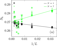
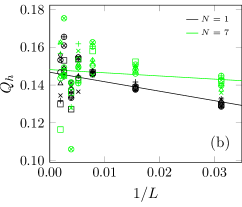
The obtained values for the width-distribution show no significant dependence on nor , our best results are and , in good agreement with those of Aarão Reis (2005).
For the distribution of surface heights, a weak correlation with the system size can be observed in Fig. 4. Heights were averaged in the steady state starting at different times (indicated by different symbols in the figure), but no dependence can be observed. Our results and are in agreement with the ranges given in Paiva and Aarão Reis (2007) and especially with the values and reported in references Marinari et al. (2000); Aarão Reis (2004). Thus all cumlant values are within error margins of the KPZ universality class irrespectively of .
III.3 Consistency of fine-size scaling with respect to DD
Since we used a parallel DD in our simulations we have also checked for dependence of the results on the applied scheme. We performed additional finite-size scaling studies with domains of and lattice sites. The figures in the parentheses refer to irregular tiling of the system. This is the consequence of the fact, that lattices cannot be divided into domains with a lateral size of six (or ten) sites without remainder, thus a subset of domains have larger lateral size to compensate it. This configuration results from dividing the system into multiples of tiles, in order to achieve optimal load balancing on NVIDIA GTX Titan Black GPUs. In both cases the smallest considered system size was to avoid unreasonable DD. Another test was done using sized domains. These tiles turned out to be too small to give correct results, expressed by failing data collapses, thus we do not consider them in the following discussion.
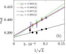
The differences among the results of the considered DD configurations were significant neither in the data collapses nor in the finite-size scaling fits. The most sensitive quantity proved to be the effective roughness exponent, shown in Fig. 5. Sample sizes of this test were smaller than those of Sec. III.2, making the extrapolations less reliable. Still, all estimates derived from this data are consistent with the estimate . Even the results of irregular, non-square DDs do not deviate significantly, although small systematic errors might be present.
IV Conclusions
Extensive numerical simulations have been performed for -dimensional RSOS models with variable height difference restrictions. Careful correction to scaling analysis has provided numerical evidence that the universal surface growth exponents agree with the most precise values known for the -dimensional KPZ class. These estimates, and , exclude the rational values and , conjectured by Kim and Kosterlitz (1989); Kim et al. (1991); Lässig (1998); Kim (2015). Our results support the generalized KPZ ansatz, which takes finite-time corrections into account and predicts exponents that are multiples of Oliveira et al. (2013). We found for and for .
We have shown that by increasing the local height differences we obtain better S/N in the simulations, but stronger corrections to scaling, which can confuse numerical analysis based on simple PL fitting. Therefore, smaller step-sized models, like the octahedron model Kelling and Ódor (2011) describe better the asymptotic, long-wave-scaling behavior of the KPZ universality class. Our conclusions for scaling corrections are in agreement with those obtained for ballistic growth models Alves et al. (2014a); Alves and Ferreira (2016). According to our knowledge oscillating convergence of effective exponents has not yet been observed in RSOS models, necessitating further investigations. We also provided estimates for the skewness and the kurtosis of the surface width distributions as well as and for the height distributions, both in the steady state. Our simulations have been performed using multisurface GPU SIMT algorithms with origin moving domain decomposition. The results have been justified by varying the tile sizes. A sustained performance of deposition attempts per second could be achieved running on a single NIVIDIA GTX Titan Black GPU. This opens up the possibility for precise RSOS simulations in higher dimensions.
Acknowledgments:
We thank S. Alves for sending us the correction-to-scaling plot of exponent of the three-dimensional ballistic growth and S. C. Ferreira and T. Halpin-Healy for useful comments. Support from the Hungarian research fund OTKA (Grant No. K109577), the Initiative and Networking Fund of the Helmholtz Association via the W2/W3 Programm (W2/W3-026) and the International Helmholtz Research School NanoNet (VH-KO-606) is acknowledged. We gratefully acknowledge computational resources provided by the HZDR computing center, NIIF Hungary and the Center for Information Services and High Performance Computing (ZIH) at TU Dresden. We acknowledge support by the GCoE Dresden. J. K. thanks M. Weigel from Coventry University for providing a guest position, co-funded through the Erasmus+ program via the Leonardo-Büro Sachsen.
References
- Kardar et al. (1986) M. Kardar, G. Parisi, and Y.-C. Zhang, Phys. Rev. Lett. 56, 889 (1986), URL http://link.aps.org/doi/10.1103/PhysRevLett.56.889.
- Halpin-Healy (1990) T. Halpin-Healy, Phys. Rev. A 42, 711 (1990), URL http://link.aps.org/doi/10.1103/PhysRevA.42.711.
- Burgers (1974) J. M. Burgers, The nonlinear diffusion equation : asymptotic solutions and statistical problems (Dordrecht-Holland ; Boston : D. Reidel Pub. Co, 1974), ISBN 9027704945, first published in 1973 under title: Statistical problems connected with asymptotic solutions of the one-dimensional nonlinear diffusion equation.
- Forster et al. (1977) D. Forster, D. R. Nelson, and M. J. Stephen, Phys. Rev. A 16, 732 (1977), URL http://link.aps.org/doi/10.1103/PhysRevA.16.732.
- Kardar (1985) M. Kardar, Phys. Rev. Lett. 55, 2923 (1985), URL http://link.aps.org/doi/10.1103/PhysRevLett.55.2923.
- van Beijeren et al. (1985) H. van Beijeren, R. Kutner, and H. Spohn, Phys. Rev. Lett. 54, 2026 (1985), URL http://link.aps.org/doi/10.1103/PhysRevLett.54.2026.
- Janssen and Schmittmann (1986) H. Janssen and B. Schmittmann, Zeitschrift für Physik B Condensed Matter 63, 517 (1986), ISSN 0722-3277, URL http://dx.doi.org/10.1007/BF01726201.
- Hwa (1992) T. Hwa, Phys. Rev. Lett. 69, 1552 (1992), URL http://link.aps.org/doi/10.1103/PhysRevLett.69.1552.
- Meakin et al. (1986) P. Meakin, P. Ramanlal, L. M. Sander, and R. C. Ball, Phys. Rev. A 34, 5091 (1986), URL http://link.aps.org/doi/10.1103/PhysRevA.34.5091.
- Barabási and Stanley (1995) A. Barabási and H. Stanley, Fractal Concepts in Surface Growth (Cambridge University Press, 1995), ISBN 9780521483186, URL https://books.google.de/books?id=W4SqcNr8PLYC.
- Krug (1997) J. Krug, Adv. Phys. 46, 139 (1997), URL http://dx.doi.org/10.1080/00018739700101498.
- Kardar (1987) M. Kardar, Nucl. Phys. B 290, 582 (1987), ISSN 0550-3213, URL http://www.sciencedirect.com/science/article/pii/0550321387902033.
- Kloss et al. (2012) T. Kloss, L. Canet, and N. Wschebor, Phys. Rev. E 86, 051124 (2012), URL http://link.aps.org/doi/10.1103/PhysRevE.86.051124.
- Schwartz and Edwards (1992) M. Schwartz and S. F. Edwards, EPL 20, 301 (1992), URL http://stacks.iop.org/0295-5075/20/i=4/a=003.
- Frey and Täuber (1994) E. Frey and U. C. Täuber, Phys. Rev. E 50, 1024 (1994), URL http://link.aps.org/doi/10.1103/PhysRevE.50.1024.
- Lässig (1995) M. Lässig, Nucl. Phys. B 448, 559 (1995), ISSN 0550-3213, URL http://www.sciencedirect.com/science/article/pii/055032139500268W.
- Fogedby (2005) H. C. Fogedby, Phys. Rev. Lett. 94, 195702 (2005), URL http://link.aps.org/doi/10.1103/PhysRevLett.94.195702.
- Canet et al. (2011) L. Canet, H. Chaté, B. Delamotte, and N. Wschebor, Phys. Rev. E 84, 061128 (2011), URL http://link.aps.org/doi/10.1103/PhysRevE.84.061128.
- Forrest and Tang (1990) B. M. Forrest and L.-H. Tang, Phys. Rev. Lett. 64, 1405 (1990), URL http://link.aps.org/doi/10.1103/PhysRevLett.64.1405.
- Halpin-Healy (2012) T. Halpin-Healy, Phys. Rev. Lett. 109, 170602 (2012), URL http://link.aps.org/doi/10.1103/PhysRevLett.109.170602.
- Marinari et al. (2000) E. Marinari, A. Pagnani, and G. Parisi, J. Phys. A 33, 8181 (2000), URL http://stacks.iop.org/0305-4470/33/i=46/a=303.
- Aarão Reis (2005) F. D. A. Aarão Reis, Phys. Rev. E 72, 032601 (2005), URL http://link.aps.org/doi/10.1103/PhysRevE.72.032601.
- Kelling and Ódor (2011) J. Kelling and G. Ódor, Phys. Rev. E 84, 061150 (2011), URL http://link.aps.org/doi/10.1103/PhysRevE.84.061150.
- Alves et al. (2014a) S. G. Alves, T. J. Oliveira, and S. C. Ferreira, Phys. Rev. E 90, 052405 (2014a), URL http://link.aps.org/doi/10.1103/PhysRevE.90.052405.
- Lässig (1998) M. Lässig, Phys. Rev. Lett. 80, 2366 (1998), URL http://link.aps.org/doi/10.1103/PhysRevLett.80.2366.
- Kim and Kosterlitz (1989) J. M. Kim and J. M. Kosterlitz, Phys. Rev. Lett. 62, 2289 (1989), URL http://link.aps.org/doi/10.1103/PhysRevLett.62.2289.
- Kim et al. (1991) J. M. Kim, J. M. Kosterlitz, and T. Ala-Nissila, J. Phys. A 24, 5569 (1991), URL http://stacks.iop.org/0305-4470/24/i=23/a=022.
- Halpin-Healy (2013) T. Halpin-Healy, Phys. Rev. E 88, 042118 (2013), URL http://link.aps.org/doi/10.1103/PhysRevE.88.042118.
- Alves et al. (2014b) S. G. Alves, T. J. Oliveira, and S. C. Ferreira, Phys. Rev. E 90, 020103 (2014b), URL http://link.aps.org/doi/10.1103/PhysRevE.90.020103.
- Pagnani and Parisi (2015) A. Pagnani and G. Parisi, Phys. Rev. E 92, 010101 (2015), URL http://link.aps.org/doi/10.1103/PhysRevE.92.010101.
- Kim (2015) J. M. Kim, J. Korean Phys. Soc. 67, 1529 (2015), ISSN 0374-4884, URL http://dx.doi.org/10.3938/jkps.67.1529.
- Alves and Ferreira (2016) S. G. Alves and S. C. Ferreira, Phys. Rev. E 93, 052131 (2016), URL http://link.aps.org/doi/10.1103/PhysRevE.93.052131.
- (33) S. Alves, private communication.
- Kelling et al. (2012) J. Kelling, G. Ódor, M. F. Nagy, H. Schulz, and K. Heinig, Eur. Phys. J.: Spec. Top. 210, 175 (2012), ISSN 1951-6355, URL http://dx.doi.org/10.1140/epjst/e2012-01645-8.
- Kelling et al. (2016) J. Kelling, M. Weigel, G. Ódor, and S. Gemming (2016), to be published.
- Ódor (2008) G. Ódor, Universality in Nonequilibrium Lattice Systems (World Scientific, 2008).
- Oliveira et al. (2013) T. J. Oliveira, S. G. Alves, and S. C. Ferreira, Phys. Rev. E 87, 040102 (2013), URL http://link.aps.org/doi/10.1103/PhysRevE.87.040102.
- Marinari et al. (2002) E. Marinari, A. Pagnani, G. Parisi, and Z. Rácz, Phys. Rev. E 65, 026136 (2002), URL http://link.aps.org/doi/10.1103/PhysRevE.65.026136.
- Foltin et al. (1994) G. Foltin, K. Oerding, Z. Rácz, R. L. Workman, and R. K. P. Zia, Phys. Rev. E 50, R639 (1994), URL http://link.aps.org/doi/10.1103/PhysRevE.50.R639.
- Paiva and Aarão Reis (2007) T. Paiva and F. Aarão Reis, Surf. Sci. 601, 419 (2007), ISSN 0039-6028, URL http://www.sciencedirect.com/science/article/pii/S0039602806010661.
- Aarão Reis (2004) F. D. A. Aarão Reis, Phys. Rev. E 69, 021610 (2004), URL http://link.aps.org/doi/10.1103/PhysRevE.69.021610.