A smooth particle hydrodynamics code to model collisions between solid, self-gravitating objects
Abstract
Context. Modern graphics processing units (GPUs) lead to a major increase in the performance of the computation of astrophysical simulations. Owing to the different nature of GPU architecture compared to traditional central processing units (CPUs) such as x86 architecture, existing numerical codes cannot be easily migrated to run on GPU. Here, we present a new implementation of the numerical method smooth particle hydrodynamics (SPH) using CUDA™ and the first astrophysical application of the new code: the collision between Ceres-sized objects.
Aims. The new code allows for a tremendous increase in speed of astrophysical simulations with SPH and self-gravity at low costs for new hardware.
Methods. We have implemented the SPH equations to model gas, liquids and elastic, and plastic solid bodies and added a fragmentation model for brittle materials. Self-gravity may be optionally included in the simulations and is treated by the use of a Barnes-Hut tree.
Results. We find an impressive performance gain using NVIDIA consumer devices compared to our existing OpenMP code. The new code is freely available to the community upon request.
Key Words.:
Methods: numerical, Planets and satellites: formation1 Introduction
Since the introduction of the first CUDA (formerly known as Compute Unified Device Architecture) development kit by the NVIDIA Corporation and even more since the support of double precision by modern GPU hardware (i.e., NVIDIA GT200 chip with compute capability of and higher), many astrophysical applications that make use of the acceleration by general-purpose computing on graphics processing units have been developed (e.g. Bédorf et al. 2012; Kulikov 2014). The modern GPUs allow for a significant performance gain compared to serial codes for central processing units (CPUs). The lower cost of GPUs compared to high performance computing clusters of CPUs leads to higher performance per cost in favor of the GPU. Moreover, GPUs are inherently more energy efficient than CPUs because they are optimized for throughput and performance per watt rather than for absolute performance (Tingxing et al., 2014). Henceforth, astrophysical problems that in general demand cluster hardware may even be addressed on workstations with NVIDIA hardware.
We decided to implement a CUDA port of our parallelized OpenMP SPH code to benefit from these modern GPUs. In this publication, we present the physical models, their CUDA implementation, the validation simulations of our new code, and we show a first glimpse at possible applications. The SPH code may be used for hydrodynamical simulations and to model solid bodies, including ductile and brittle materials. The code uses a tree code algorithm for the additional treatment of self-gravity. We show several validation simulations: the simulation of elastic rubber cylinders, the gravitational collapse of a molecular cloud, the impact of an aluminium bullet into an aluminium cube and the impact of a nylon bullet in a basaltic rock.
Extended hydrocodes have been applied to model large deformation and strong shock wave physics using different numerical schemes. The Eulerian grid code CTH has several models that are useful for simulating strong shock, large deformation events, and this code can be used to model elastic-plastic behavior and fracture (McGlaun et al., 1990). The iSALE grid code is a comprehensive tool to study impacts (Wünnemann et al., 2006; Elbeshausen et al., 2009). Apart from grid codes, there are also particle-based numerical schemes. Several SPH codes for modern cluster hardware are available to the community. The well-known Gadget-2 code by Springel (2005) may be the most sophisticated and most widely applied SPH code for the simulation of astrophysical flows. The SPH code by Benz & Asphaug (1994) with fundamental improvements of the physical models later by Jutzi et al. (2008) has been successfully applied to simulate impacts and collisions of astrophysical objects. However, there is no freely available SPH code for the simulation of solid and brittle material including the treatment of self-gravity at hand. Our new code bridges this gap and high resolution SPH simulations become feasible and may be performed even on a standard workstation with a GPU from the consumer price range.
The outline is as follows. In the next section we present the physical models and the governing equations that are solved by the code. In sect. 3 we describe the smooth particle hydrodynamics numerical model for the simulation of solid bodies, the Grady-Kipp damage model for the formation of cracks and stress weakening, and the Barnes-Hut tree algorithm for gravitational forces. We give a detailed description of our implementation of these algorithms in the new CUDA code. We present the results of three standards tests for the code in sect. 4: the collision of two perfect elastic rubber cylinders, the high-velocity impact of a bullet into an aluminium cube, and the collapse of an isothermal molecular cloud. Our first application of the new code s described in sect. 5 and we present its results in sect. 6 where we additionally discuss the limitations of the current code version in regard to numerical issues as well as in terms of the physical models. Eventually, we conclude in sect. 7.
2 Physical model
In this section, we present the set of partial differential equations from continuum mechanics in Cartesian coordinates that we apply to model gas and solid bodies. Throughout this paper, the Einstein summation rule is used, Greek indices denote spatial coordinates and run from 1 to 3.
2.1 Mass conservation
The equation of continuity is the equation of the conservation of mass. It is given in Lagrangian form by
| (1) |
where denotes the density and the velocity of the solid body or fluid.
2.2 Conservation of momentum
The equation of the conservation of momentum in continuum mechanics for a solid body reads in Lagrangian formulation
| (2) |
where is the stress tensor given by the pressure and the deviatoric stress tensor
| (3) |
with the Kronecker delta . For a liquid or gas, the deviatoric stress tensor vanishes and the conservation of momentum is given by the Euler equation
| (4) |
2.3 Conservation of internal energy
The equation of the conservation of the specific internal energy for an elastic body is given in Lagrangian formulation by
| (5) |
with the strain rate tensor given by eq. (8).
2.4 Constitutive equations
In contrast to fluid dynamics, the set (1;2;5) of partial differential equations is not sufficient to describe the dynamics of an elastic solid body, since the time evolution of the deviatoric stress tensor is not yet specified. For the elastic behavior of a solid body, the constitutive equation is based on Hooke’s law. Extended to three dimensional deformations, it reads
| (6) |
Here, denotes the material dependent shear modulus and is the strain tensor. For the time evolution, it follows (for small deformations)
| (7) | ||||
where denotes the strain rate tensor, given by
| (8) |
The rotation terms in eq. (7) are needed since the constitutive equations have to be independent from the material frame of reference. There are various possibilities to achieve this. The usual approach for particle codes is the Jaumann rate form (see, e.g., Gray et al. 2001 and references therein). The rotation terms of the Jaumann rate form are
| (9) |
with the rotation rate tensor
| (10) |
Together, eqs. (7) and (9) determine the change of deviatoric stress due to deformation of the solid body.
2.5 Equation of state
The equation of state relates the thermodynamic variables density , pressure , and specific internal energy . We provide a short description about the equation of states that are implemented in the code.
2.5.1 Liquid equation of state
For small compressions and expansions of a liquid, the pressure depends linearly on the change of density. Assume is the initial density of the uncompressed liquid. Then, the liquid equation of state reads
| (11) |
Here, denotes the bulk sound speed of the liquid, which is related to the bulk modulus and the initial density by
| (12) |
If the density falls strongly beyond the value of the initial density , the liquid equation of state fails because the liquid forms droplets and attracting forces vanish. To account for this behavior, the pressure is set to zero as soon as the ratio drops below (Melosh, 1996).
2.5.2 Murnaghan equation of state
The Murnaghan equation of state is an extension of the liquid equation of state (see, e.g., Melosh 1996). In contrast to the liquid equation of state, the pressure now depends nonlinearly on the density
| (13) |
with the zero pressure bulk modulus and the constant . The Murnaghan equation of state is limited to isothermal compression. Parameters for various materials can be found in the literature, e.g., Melosh (1996).
2.5.3 Tillotson equation of state
The Tillotson equation of state was originally derived for high-velocity impact simulations (Tillotson, 1962). There are two domains depending upon the material specific energy density . In the case of compressed regions () and lower than the energy of incipient vaporization the equation of state reads
| (14) |
with and . In case of expanded material ( greater than the energy of complete vaporization ) the equation of state takes the form
| (15) |
The symbols , , , , , , , and are material dependent parameters.
In the partial vaporization , is linearly interpolated between the pressures obtained via (14) and (2.5.3), respectively. For a more detailed description see Melosh (1996).
The Tillotson equation of state has the advantage of being computational very simple, while sophisticated enough for the application over a wide regime of physical conditions, such as high-velocity collisions and impact cratering.
2.6 Plastic material equations
Together with the equation of state, the set of equations (1;2;5) can be used to describe the dynamics of a solid body in the elastic regime. We apply the von Mises yield criterion (von Mises, 1913) to model plasticity. The deviatoric stress is limited by
| (16) |
where the factor is computed from
| (17) |
with the second invariant of the deviatoric stress tensor given by
| (18) |
and the material dependent yield stress is .
2.7 Damage model for brittle material
Since one major application of the newly developed code includes the simulation of the collision between brittle planetesimals, we included a fragmentation model. Physically, fracture is related to the failure of atomic or molecular bonds. If an applied force on a solid brittle body is large enough to break the atomic bonds, the material begins to fracture and develop cracks. A successful continuum model for fragmentation was derived by Grady & Kipp (1980) and first implemented in a SPH code by Benz & Asphaug (1995). The model is based on two assumptions: brittle materials contain so-called flaws that are sources of weakness leading to activation and growth under tensile loading, and dynamic fracture depends on the rate of tensile loading. In other words, material that is slowly pulled apart develops fewer cracks than material that experiences higher strain rates, since one single crack cannot relieve the higher tensile stress, and hence more flaws get activated leading to more cracks and consequently more damage.
The scalar parameter damage parametrizes the influence of cracks on a given volume
| (19) |
and is defined in a way that represents an undamaged, intact material and a fully damaged material that cannot undergo any tension or deviatoric stress. In this manner, a material with experiences half the stress and tension of undamaged material with .
Damage reduces the strength under tensile loading and the elastic stress is decreased by the factor , or in more detail
| (20) |
with
| (21) |
The number of flaws per unit volume in a brittle body with failure strains that are lower than , is given by the Weibull distribution (Weibull, 1939)
| (22) |
with the two Weibull parameters and . Typical values for basalt are , (Nakamura et al., 2007).
As soon as a spherical volume undergoes a strain greater than its lowest activation threshold strain, damage starts to grow according to
| (23) |
with the constant crack growth velocity . The crack growth velocity is chosen to be 40% of the velocity of a longitudinal elastic wave in the damaged material
| (24) |
The fracture model requires the distribution of activation threshold strains over the brittle body as a preprocessing step to the simulations. We show how we achieve this in sect. 3.2.
3 Numerical model and implementation
In this section, we describe the numerical models that are implemented in the CUDA code.
3.1 Smooth particle hydrodynamics
Smooth particle hydrodynamics is a meshless Lagrangian particle method that was first introduced by Lucy (1977) and Gingold & Monaghan (1977) for the solution of hydrodynamic equations for compressible flows in astrophysical applications. The SPH method was extended to model solid bodies at the Los Alamos National Laboratory. This work was pioneered by Libersky & Petschek (1991) with various improvements from the same source later on (Randles & Libersky, 1996; Libersky et al., 1997). The first astrophysical application of SPH with strength of material was by Benz & Asphaug (1994). Our implementation of the SPH equations in the code mainly follows their work.
For a comprehensive introduction to the basic SPH idea and algorithm, we refer to the excellent publications by Benz (1990) and Monaghan (1992). In this section, we present the SPH equations that we have implemented in the CUDA code, since more than one equivalent SPH representation exists for the partial differential equations considered in this work.
In the following, roman indices , denote particle indices and the sum in a SPH equation runs over all of the interaction partners.
3.1.1 Kernel function
The standard kernel, which is widely used in the astrophysical SPH community and in our CUDA code, is the cubic B-spline function introduced by Monaghan & Lattanzio (1985). This function is written as
| (25) |
where is the distance between two interacting particles, denotes the smoothing length, and is a normalization constant depending on the dimension
| (26) |
The first derivative of the kernel is given by
| (27) |
3.1.2 SPH equations
In most astrophysical applications of SPH to hydrodynamical problems, the continuity equation (1) is not solved. The density of one particle is given directly by the kernel sum
| (28) |
We use eq. (28) for purely hydrodynamical problems as well and to calculate the densities during the gravitational collapse of a molecular cloud in sect. 4.2.
To model solid bodies, however, it is often more convenient to integrate the continuity equation using the following SPH representation: the change of the density of particle is given by (Gray et al., 2001)
| (29) |
In order to calculate the acceleration for particle , we use the SPH representation of the equation of motion (2)
| (30) |
We add some additional artificial terms to eq. (30) in the following sections to avoid some numerical issues of the algorithm.
Finally, the equation for the time evolution of the specific internal energy reads in SPH representation
| (31) |
3.1.3 Artificial viscosity
An important issue is the artificial viscosity. In order to treat shock waves in an ideal fluid, dissipation is needed to dissipate kinetic energy in the shock front. In SPH, it is necessary to prevent the particles from unphysical mutual penetration. The artificial viscosity terms were introduced by Monaghan & Gingold (1983). They can be regarded as an additional artificial pressure term in the equations for the conservation of momentum and energy. The additional pressure is calculated for each interaction pair and as follows:
| (32) |
where and are free parameters that determine the strength of the viscosity, and and are the averaged quantities for density and sound speed for the two interacting particles, and .
The term is an approximation for the divergence and is calculated accordingly
| (33) |
Here, is the average of the smoothing length of particle and . The term in the denominator prevents divergence of for particles with small separations.
The artificial pressure is added to the acceleration of the particle
| (34) |
with for and elsewhere. This means, the artificial viscosity leads to a repellent force only for approaching particles.
3.1.4 Artificial stress: Tensile instability
The tensile instability can occur in SPH simulations that include materials with equation of states that allow negative pressure or tension. In the worst case, the instability leads to artificial numerical clumping of particles and in the end to unnatural fragmentation. There are several different approaches to overcome the tensile instability. In our code, we have implemented an additional artificial stress. To avoid artificial clumping of particles due to the tensile instability of the SPH method, Monaghan (2000) added a small repulsive artificial stress to the SPH equation (30)
| (35) |
The artificial stress is given by the sum of the artificial stress for particle and , respectively,
| (36) |
with for tension
| (37) |
whereas for compression. The factor is typically around . The repulsive force that results from the artificial stress is scaled with , with , where is given by the ratio between the kernel for the interaction of particles and and , the mean particle distance in the vicinity of particle ,
| (38) |
The usual approach is to take the mean particle distance of the initial particle distribution for . The artificial stress leads to an additional repulsive force whenever tension would trigger the tensile instability. The effect of artificial stress is shown in an illustrative example in sect. 4.1.
3.1.5 XSPH — The Velocity
The time derivative of the location of particle is given by the velocity of particle
| (39) |
However, the velocity of the continuum cannot necessarily be identified with the particle velocity. The XSPH algorithm (Monaghan, 1989) moves the particles at an averaged speed smoothed by the velocity of the interaction partners
| (40) |
Here, the factor is called the XSPH factor, . Throughout our simulations performed for this paper, we set when we use XSPH.
3.1.6 A note on linear consistency
In standard SPH, the velocity derivatives in eq. (8) for the determination of the strain rate tensor for particle are given by
| (41) |
This approach, however, leads to erroneous results and does not conserve angular momentum due to the discretization error by particle disorder in simulations of solid bodies. This error can be avoided by constructing and applying a correction tensor (Schäfer et al., 2007)
| (42) |
where the correction tensor is given by the inverse of
| (43) |
and it holds
| (44) |
We apply the correction tensor according to eq. (42) in all our simulations that demand for derivatives of the velocity to force first order consistency.
3.2 Damage model
As a preprocessing step to a simulation containing brittle materials, we have to distribute activation threshold strains or flaws among the SPH particles. We apply the algorithm introduced by Benz & Asphaug (1995) with the following approach: Flaws are distributed randomly among the brittle particles until each particle has been assigned with at least one activation threshold. We let be the number of totally distributed activation flaws. For each flaw , , a particle is chosen randomly and assigned with the activation threshold strain derived from the Weibull distribution ,
| (45) |
where is the volume of the brittle material and and are the material dependent Weibull parameters. Using this procedure, each particle gets at least one flaw and on average a total of flaws are distributed. This number of flaws has to be stored in the memory during the simulation and is the main memory consumer in simulations with brittle materials.
During the simulation, once a particle undergoes a strain greater than its lowest activation threshold strain, damage grows according to a modified version of eq. (23)
| (46) |
where is the number of activated flaws of the particle. This modification accounts for the accumulation of cracks.
Additionally, a damage limiter is included in the model. Since a particle has in general more than only one activation threshold, its behavior under tensile loading would be given by the flaw with the lowest activation threshold. To prevent this, the damage of the particle is limited by the ratio between the number of activated flaws and the number of total flaws of this particle
| (47) |
In other words, a particle can only be totally damaged if all of its flaws are activated.
In order to determine if a particle exceeds one of its threshold strains during the simulation, we need to derive the local scalar strain from the three-dimensional stress. Benz & Asphaug (1995) suggest computing the local scalar strain from the maximum tensile stress , where are the principal stresses determined by a principal axis transformation of the stress tensor , which is already reduced by damage and yield strength
| (48) |
The Young’s modulus of the intact material given by the bulk and shear moduli is written as
| (49) |
3.3 Barnes-Hut tree
We have implemented the efficient routines for Barnes-Hut tree builds and calculation of the gravitational forces for GPUs introduced by Burtscher (2011). The algorithm for the tree generation is explained in sect. 3.5.1.
Barnes & Hut (1986) were the first to use a hierarchical tree to calculate the gravitational forces between N bodies. Their approximation algorithm uses a tree-structured hierarchical subdivision of space into cubic cells, each of which is divided into subcells. The algorithm has the order compared to the algorithm of the direct sum. The basic idea is that only nearby particles have to be treated individually during the calculation of the gravitational force on a specific particle. Distant nodes of the tree can be seen as one single particle sitting at the center of mass of the specific tree node and carrying the mass of all the particles that reside in this node. Although different algorithms for the computation of self-gravitational forces exist, the hierarchical tree method is specially suited for the use in combination with SPH. As a side product of the computation of the gravitational forces, the hierarchical tree is constructed for each individual time step and hence, a geometrical hierarchy of the SPH particles (leaves of the tree) is available at all time of the computation. It can be used to determine the interaction partners for the SPH algorithm by performing a tree walk for each individual particle (Hernquist & Katz, 1989). Although the tree walks may take longer than the search through a helping grid, the interaction partner search may be faster because, in any case the tree build needs to be carried out in simulations with self-gravity.
We calculate the center of mass and total mass of every node in the tree to calculate the gravitational force exerted on the SPH particles. We call these objects pseudo-particles in the following. Now, for each SPH particle, we perform a tree walk over all nodes. With the use of the criterion, we identify whether a pseudo-particle sitting in the node may be used for the calculation of the gravitational force acting on our particle or whether we have to descend further down in the tree. The criterion is given by
| (50) |
where denotes the edge length of the tree node containing the pseudo-particle and is the distance between the SPH particle and the pseudo-particle. The gravitational force from the pseudo-particle acting on the particle is then given by
| (51) |
where and denote the location and the mass of the pseudo-particle, respectively. To avoid numerical instabilities, the distance between the pseudo-particle and the particle is smoothed.
Barnes & Hut (1989) present a detailed error analysis for their tree algorithm. They find consistent accuracies of the algorithm for with the consideration of the monopoles of the tree compared to and the additional calculation of the quadrupoles for each tree node. The error scales with and . For the sake of memory saving, we calculate only the monopoles of the tree and use in our simulations including self-gravity instead of the usual value of .
3.4 Time integration
An important subset of every SPH code is the time integration function. We have implemented two different time integrators for the code: a predictor-corrector algorithm following the publication by Monaghan (1989) and a Runge-Kutta 3rd order integrator with adaptive time step control. In the following, we present the basic algorithm for the integrators and the time step control mechanisms.
3.4.1 Predictor-corrector
A simple predictor-corrector integration scheme is implemented in the code as follows. We let be a quantity that is integrated in time and its derivative. At first we perform a prediction integration step and calculate the value after half the time step ,
| (52) |
Now, we use the predicted values to calculate the time derivatives for the correction step and based on them the new values ,
| (53) |
Obviously, the time step has to be limited. To set an upper limit to the time step we use the following condition from the acceleration:
| (54) |
and the Courant condition
| (55) |
The maximum time step for this integration step is then given by
| (56) |
Additionally, we allow only a maximum change for all other quantities that are integrated. This may be necessary for quantities, such as the density, stress, internal energy, and damage, and is written as
| (57) |
3.4.2 Embedded Runge-Kutta integrator
In addition to the predictor-corrector scheme, we also implemented a more sophisticated Runge-Kutta integration scheme that features an adaptive step size control. The basic algorithm is based on a Runge-Kutta 3rd order scheme where the third step that is used to give an error estimate about the quality of integration step; see Abramowitz & Stegun (1964) and especially Butcher (1987) for a more detailed description. The great advantage of this scheme lies in the possibility of setting a maximum relative error for the quantities since the Courant condition, in principle, is only applicable in hydrodynamical simulations.
The standard 3rd order Runge-Kutta integration scheme for a quantity , which is integrated in time from to , is written as
| (58) |
with and .
Writing the three substeps are given by
| (59) | ||||
| (60) | ||||
| (61) |
The quantity can also be integrated using the Euler midpoint method. There, the value at time is given by
| (62) |
Now, we use the difference between and to give an estimate for the local error of the scheme by comparison to the value resulting from an Euler step
| (63) |
If is smaller than the desired relative error defined in the configuration file , the integration step is accepted and the time step size is increased to
| (64) |
If the error is too large, the time step size is decreased accordingly to
| (65) |
3.5 Implementation in CUDA
In this section, we present how we have implemented the numerical algorithms from the last section for the NVIDIA GPUs with CUDA. Depending on the problem, the information about the particles is stored in one-dimensional arrays, e.g., posx[], posy[], posz[], velx[], vely[], velz[], and stress[]. The bottleneck for GPU computation is the slow memory bandwidth between host and device. Therefore, we initially copy all particle data to the GPU and perform all calculations with the SPH particles there. After certain time frames the data is written to the hard disk in an additional POSIX thread to avoid that the computation time depends on disk i/o for simulations with high output.
3.5.1 Barnes-Hut tree
We have implemented the Barnes-Hut tree strictly following the efficient implementation for N-body calculations with CUDA by Burtscher (2011). The hierarchical decomposition is recorded in an octree. Since CUDA does not allow the use of pointers, which is convenient for the handling of trees, e.g., allows for recursive programming of tree walks, we use one large index array for all SPH particles and all tree nodes, which we call childList. This memory is allocated dynamically at the start of the simulation run. The maximum number of tree nodes is given by , where is the number of SPH particles in the simulation. For each tree node there are entries in childList, where is simply given by the dimension
| (66) |
The tree is constructed in a way that the particles reside in leaves in the end. At first, the root of the tree is constructed from the geometry of the particle distribution. The computational domain (in three dimensions) is given by the cube, which encloses all SPH particles. This cube has the edge length
| (67) |
and defines the edge length of the root node. The edge length of a tree node of depth is given by
| (68) |
Starting from the root node, the particles are inserted into the tree in the following way. In the beginning, all but one (the root node) entry in childList are , corresponding to the status ”no kid”. All particles are distributed among the threads on the GPU. Now threads on the GPU start to compare the locations of their SPH particles with the position of the root node to determine the childindex. Since there are many more threads than children (especially in the beginning of the algorithm), we need to avoid race conditions actively. To accomplish this, we add the status or ”locked” to the childList and use the CUDAfunction ”atomic compare and save” atomicCAS to lock an entry in the childList. This functions checks first if the specific index is already locked. If the index in childList is already locked, the thread waits for the other threads to finish and restarts its attempt. If the index is not locked, the threads read the index value, which may be in the beginning or a different node index, and saves it. Now, the second round starts and the children of the root node are already filled with SPH particles that were sorted there. Since leaves or particles cannot have children by definition, new inner tree nodes have to be generated. A new inner tree node has half of the edge length from its parent. New inner tree nodes are added until both particles, the new particle and the particle in the parent node, can be sorted into two different leaves. As soon as both particles reside in different leaves, the thread writes and cancels the lock.
When we want to calculate the gravitational forces between the SPH particles, we have to calculate the positions and locations of the pseudo-particles in the tree. We use the algorithm presented by Burtscher (2011) in the following manner to determine the pseudo-particle in a specific node: For each inner node, we start in parallel for a CUDA kernel that picks the last added inner nodes, for which we calculate the center of mass and total mass at first. If the inner nodes are not leaves, the thread looking at these nodes and has to wait for all other threads to end beforce continuing because it needs the location and mass of the pseudo-particles in these nodes. This is again done by the use of as the initial mass of a pseudo-particle. When the thread finishes the calculation for its node, it moves up one tree depth and continues with the next node. The implementation of Burtscher is especially designed for CUDA, regarding memory access and parallelization.
3.5.2 Neighbor search
One major task in a SPH code is to find an efficient way to determine the interaction partners for each SPH particle for the kernel sums. Normally, the fastest way to obtain the interaction partner list in a SPH simulation with one fixed smoothing length is via an additional helping grid with a grid size of the smoothing length. Then all particles are sorted into the grid, and only the neighboring grid cells have to be searched for interaction partners. There are numerous publications about the best way to implement a searching grid in SPH, and we refer to the nice overview given in Speith (1998).
Since we already computed the Barnes-Hut tree for the calculation of self-gravity, we can easily benefit and use the tree to determine the interaction partners without any additional helping grid. The tree search is implemented in the following way: Corresponding to the childList for the tree, we also have an index array that stores the information about the interaction partners, interactionsList. In contrast to the tree generation algorithm, there are no race conditions in the interaction partner search algorithm, since we can search for the interaction partners of particle independently from the search of particle . Each thread searches for its particles and starts the search for each particle at the root node. If the particle lies within the cube of edge length
| (69) |
we descend into the children and continue searching. As soon as a leaf, that is a different particle, is encountered, we check whether the distance between the leaf and particle is smaller than the smoothing length, and if so, the index of the leaf is added to the interactionsList accordingly.
Since all threads are independent in this algorithm, it is very efficient and fast.
3.5.3 Smooth particle hydrodynamics equations
The CUDA implementation of the SPH sums for the equation of motion and conservation of energy is straightforward, since as soon as the interaction partners for each particle are known, the computation of these quantities can be performed independently.
4 Numerical tests and code validation
In this section, we present some of our numerical tests that we performed for code validation. We chose three standard cases to test the different aspects of the code.
4.1 Colliding rubber cylinders
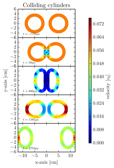
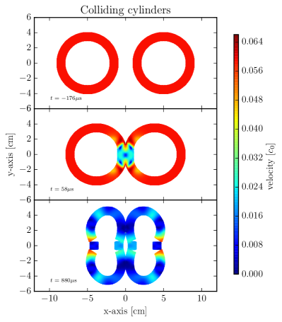
A suitable test for the correct implementation of the tensile instability fix is the simulation of two colliding rubber cylinders. As first presented by Swegle (1992), the collision results in fragmentation, especially when the particles are initially placed on a squared grid. We use the setup by Monaghan (2000) and Gray et al. (2001), and use following material parameters and units: The unit of density is , the unit of length is , the unit of velocity is ( ), and the unit of stress is . The value of the shear modulus is set to . We use two rubber cylinders with inner radius and outer radius , moving initially in one direction with , so that the collision velocity is . In order to test the implementation of artificial stress, we perform two different simulations: We set the parameters for the artificial stress to and in one simulation, while we do not add any artificial stress in the other run. Additionally, XSPH is applied with and the artificial viscosity coefficient is set to in both setups.
The results of the simulations with and without artificial stress are shown in fig. 1 and 2, respectively. In the case without any artificial stress, the cylinders fracture shortly after maximum compression. In the simulation with artificial stress, the cylinders bounce off each other without fracturing and begin to swing. The timescale is chosen according to Monaghan (2000) for best comparison. The cylinders touch at .
4.2 Gravitational Collapse of a Molecular Cloud
In order to test the gravitational tree algorithm in the code, we run the standard test case for self-gravitating objects presented by Boss & Bodenheimer (1979). These authors investigated the collapse of a self-gravitating, initially spherical, and uniformly rotating gas cloud. Internal pressure is included, but viscous and magnetic forces are neglected. The collapse of the cloud is considered to be isothermal. The equation of state is that of an ideal gas of pure molecular hydrogen with constant temperature . The initial conditions are as follows: the total mass of the molecular cloud is , the mean density is given by , the molecular cloud rotates uniformly with the angular velocity , and the initial radius of the spherical cloud is .
A nonaxisymmetric perturbation of mode and amplitude depending on the azimuthal angle is superposed on the initially uniform density
| (70) |
The free-fall time is given by
| (71) |
We performed several simulations with different number of particles, ranging from to . We varied the type of smoothing of the gravitational forces. Since the mean particle distance rapidly shrinks during the simulation, it is convenient to use a variable smoothing length and a constant number of interaction partners. The kernel value for the interaction of particle and is then calculated with the mean smoothing length
| (72) |
To enforce a constant number of interaction partners per particle, we start with the smoothing length of the last time step and iterate using the new smoothing length (Hernquist & Katz, 1989)
| (73) |
where is the desired number of interaction partners and the actual number of interaction partners gained with the smoothing length .
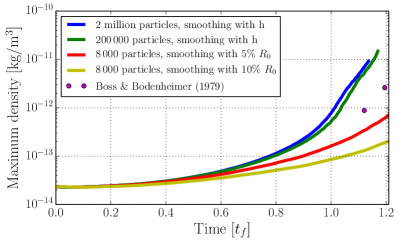
The results of our simulations are in very good agreement to previous calculations by Boss & Bodenheimer (1979). Moreover, in accord with Bate & Burkert (1997) we find differing collapse speeds depending on the smoothing of the gravitational potential.
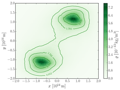
Figure 3 shows a color-coded plot of the density in the midplane after a simulation time of approximately the free fall time for the simulation with two million SPH particles. There is already an increase of density of almost two orders in magnitude at the location of the initial perturbation, where the two protostars are about to form.
Figure 4 shows the evolution of the maximum density during the collapse for different setups and smoothing of the gravitational force. In order to estimate the maximum density, we mapped the SPH particles on a cubic grid to compare our results to the grid code results by Boss & Bodenheimer (1979). Since our spatial resolution is much better than the resolution from the coarse simulations 30 years ago, we obtain a higher maximum density. Accordingly, we find a slower evolution of the maximum density in our (very) low resolution simulations including particles. Another major influence on the density evolution is found in the smoothing of the gravitational forces. In order to avoid numerical instabilities due to close encounters of two particles, eq. (51) has to be modified and the distance between two bodies is smoothed. We applied three different smoothing schemes for best comparison to the former publications. The first smoothing algorithm sets the smoothing length as the lowest possible distance between two particles. This algorithm was used in the simulation with two million particles. Another ansatz is to add an additional tiny distance to in (51) regardless of the separation between two gravitational objects. The values for this tiny distance employed by Bate & Burkert (1997) are % and % of the initial radius of the molecular cloud. Using these different smoothing methods, we receive the density evolutions presented in figure 4.
4.3 Impact cratering: Comparison to experiment
Prater (1970) performed several experiments of high-velocity impacts in different aluminium alloys. To validate our code for the use of impact modeling, we simulated the impact of an aluminium alloy 6061 bullet with radius in an aluminium alloy 6061 cube with an impact speed of . We then compared our results to Pierazzo et al. (2008). Since aluminium is not a geological material, this simulation was performed without the use of the Grady-Kipp damage model, solely with the von Mises plasticity model. The three-dimensional simulation has the following initial setup: We use SPH particles for the cube and particles for the impacting bullet, the numerical parameters are , , and the material parameters are , , , and . The parameters for the Tillotson equation of state , , , , , , , , are , , , , , , , and , respectively. The surface of the cube with the crater after the impact is shown in figure 5.
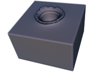
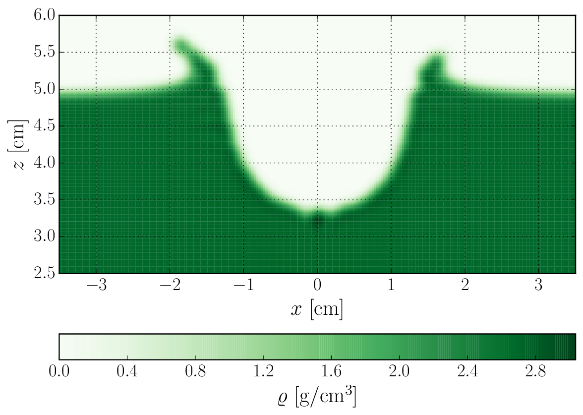
The dimensions of the final crater can be seen in figure 6. They are in good agreement with the numerical results by Pierazzo et al. (2008) and the experimental results by Prater (1970).
4.4 Damage model: Comparison to experiment
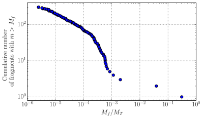
We simulated a laboratory impact experiment into a basaltic rock performed by Nakamura & Fujiwara (1991) to test the implementation of the damage model. In their experiment, a small nylon bullet impacts with an impact speed of into a basaltic rocky sphere with a diameter of . We chose to simulate an off-axis impact with an impact angle of (see fig. 9 for the definition of the impact angle), which corresponds to an impact parameter of 25% of the diameter. We modeled the basalt target with particles and applied the Tillotson equation of state. Owing to the lack of parameters for nylon, we used lucite for the projectile material (values were taken from (Benz & Asphaug, 1994)). The basalt target was modeled with the additional damage model and activation threshold strains were distributed following the Weibull distribution statistically as a preprocessing step (see sect. 3.2 for a detailed description of the algorithm). Following Benz & Asphaug (1994), we performed several simulations with varying Weibull parameter pairs and . Figure 7 shows the damage pattern in the target after for the simulation that matched the experimental outcome best. The damage in the region around the impact point is the largest and all particles close to the impact point were immediately damaged upon impact. The damage pattern is radially symmetric around the impact point. Another source of damage is found near the surface of the target. There, damage grows due to spallation stresses that occur when compressive waves get reflected at the free surface. As a result of this nature, the inner core of the target remains intact while the surface is coated with cracks. After simulation time, the damage pattern in the target remains unchanged. We identified single fragments using a friend-of-friend algorithm in the following way: First, we removed all fully damaged particles. Then, we clustered all remaining particles that are closer than of the original smoothing length to their neighboring particles. Fragments consisting of less than three particles were neglected. Figure 8 shows the fragment mass spectrum obtained with this friend-of-friend clustering algorithm.
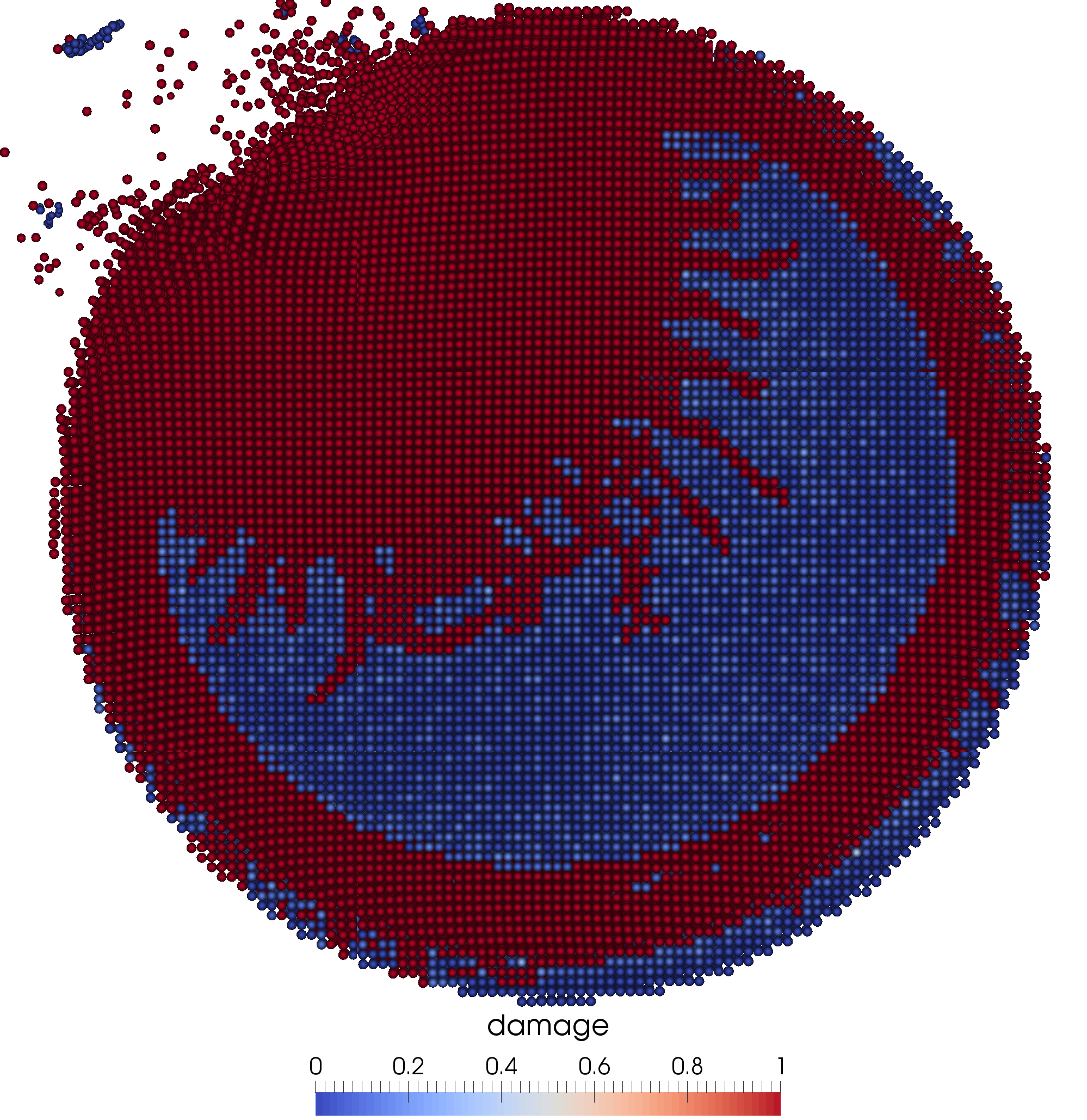
We find best agreement of the remaining target core size to the experimental data for and , which is close to the values and found by Benz & Asphaug (1994). The intact core incorporates of the initial target mass, which has to be compared to the experimental value of .
5 Collision between Ceres-sized objects and water transport
In a forthcoming paper, we study the transfer of water during collisions of Ceres-sized bodies based on preliminary results obtained with our previously presented OpenMP SPH code (Maindl et al., 2013, 2014) and new, higher resolution simulation results gained from the code described here. While Marcus et al. (2010) show that water contents cannot increase from giant impacts involving bodies with masses between 0.5 M and 5 M, we are interested in possible water delivery by impacts in early planetary systems and hence collision events of smaller bodies, typically involving lower energy and the possibility of water (ice) being transferred between the impactors. Many existing planet formation studies (e.g., Dvorak et al., 2012; Raymond et al., 2004; Izidoro et al., 2013) assume perfect merging and complete delivery of the asteroids’ and planetesimals’ water contents to the impact target. As this assumption does not hold, we need to closely investigate the impact process itself to define conditions under which water is actually transferred rather than lost during a smaller scale collision. By including a realistic water transfer and loss model in planet formation studies the actual amount of water on the final stages of terrestrial planets may be smaller by a factor of 5–10 (Haghighipour & Raymond, 2007). Most simulations of giant impacts use a strengthless material model (e.g., Canup et al., 2013) based on self-gravity dominating the material’s tensile strength beyond a certain size of the colliding bodies (400 m in radius; Melosh & Ryan, 1997). We study collisions of Ceres-sized objects the size of which is just about on the verge of gravity domination and we expect more realistic results from including solid body dynamics as put forth in sect. 2.
In this section we present first results from the mentioned higher resolution simulations using the subject CUDA code.
5.1 Scenario setup
The collision scenarios include two spherical objects composed of basaltic rock and water ice. Target and projectile have one Ceres mass () each. The target has a basaltic core with a 30 wt-% water ice mantle and the projectile consists of solid basalt. Owing to the different densities, this configuration results in target and projectile radii of and , respectively. Upon contact, the mutual escape velocity of the two bodies is . Neither of the bodies is rotating at the start of the simulation.
For modeling the materials we use the Tillotson equation of state (see sect. 2.5.3) with material parameters as listed in Benz & Asphaug (1999) and our table 1. The damage model (cf. sect. 3.2) is implemented with Weibull parameters, which were measured for basalt by Nakamura et al. (2007), and for water ice we adopt values mentioned in Lange et al. (1984); see table 2.
| Material | ||||||||||||
|---|---|---|---|---|---|---|---|---|---|---|---|---|
| [] | [GPa] | [GPa] | [] | [] | [] | [] | [] | |||||
| Basalt | 2700 | 26.7 | 26.7 | 487 | 4.72 | 18.2 | 0.5 | 1.50 | 5.0 | 5.0 | 22.7 | 3.5 |
| Ice | 917 | 9.47 | 9.47 | 10 | 0.773 | 3.04 | 0.3 | 0.1 | 10.0 | 5.0 | 2.8 | 1 |
| Material | [] | Reference | |
|---|---|---|---|
| Basalt | 16 | Nakamura et al. (2007) | |
| Ice | 9.1 | Lange et al. (1984) |
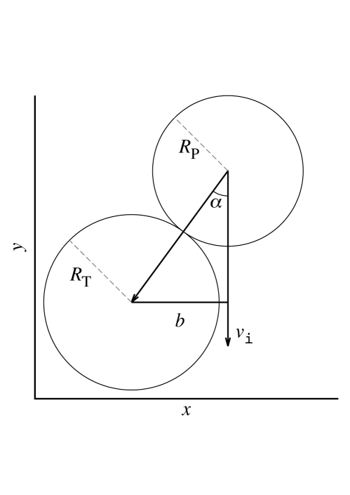
Here we present results for a specific hit-and-run collision simulated with a resolution of SPH particles. The projectile and target start apart with an initial impact parameter of and a relative velocity of . While the individual bodies’ SPH particle distributions were relaxed and in equilibrium before the simulation, we chose this relatively large initial separation of the bodies to allow for a realistic modeling of tidal effects during their mutual approach. Under the influence of the initial momenta and self-gravity the actual collision happens into the simulation. The impact velocity is and the impact angle . The latter is measured such that a head-on collision corresponds to ; figure 9 illustrates the collision geometry. These impact characteristics are definitely in the hit-and-run domain of the collision outcome map (see e.g., Leinhardt & Stewart 2012), hence we expect two major survivors that escape each other. In order to be able to clearly identify the surviving bodies and to cover the complete collision process, we simulate for system time.
5.2 Results
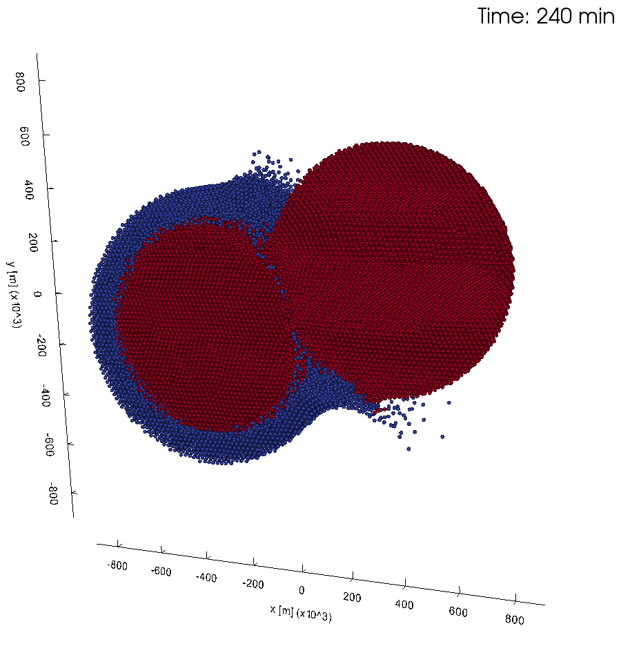
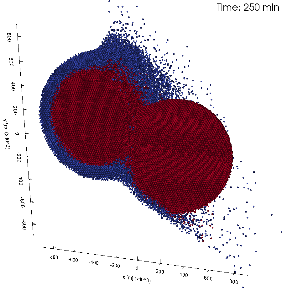
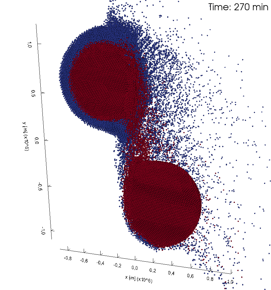
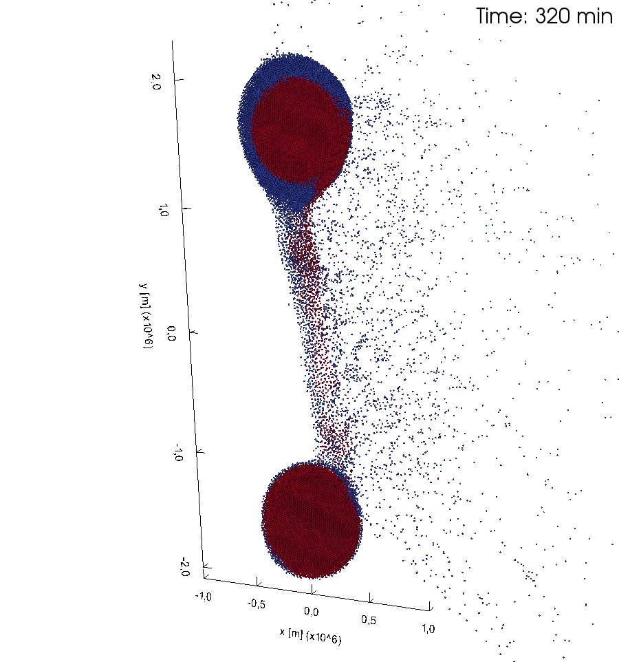
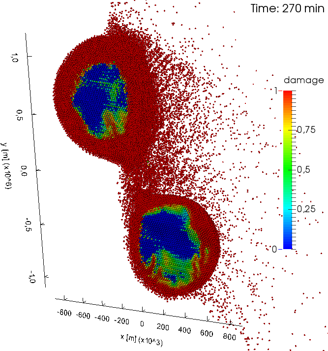
The simulation results in two surviving bodies of about equal mass that escape each other, as expected for a hit-and-run scenario. Figure 10 shows snapshots from the collision until about after, a time when the two bodies are clearly separated again, but still connected by a debris bridge. At the collision site, the icy mantle of the target is stripped and exposes the rocky core. Is it also notable that the initially dry projectile accretes some of the water originally in the target’s mantle. The spread-out debris is either reaccreted by one of the two major survivors or it forms fragments.
After the simulation timespan of , the two big objects reach a mutual distance of more than . At this point, we identify the surviving fragments using a friends-of-friends algorithm with the smoothing length as the linking length and find a sharp decrease in mass beyond the two main survivors and . In total there are 2503 fragments, most of them consisting of one to few SPH particles. In order for to qualify as a “significant fragment”, we require that it consists of at least 20 SPH particles. Table 3 lists the surviving six significant fragments and illustrates the sharp decline in their size beyond the two major survivors. Given the differing mass of icy and rocky SPH particles by a factor of about three, the number of particles in a fragment is not necessarily proportional to its mass. Beyond the two main bodies, the clumps consist of just barely over 20 SPH particles so that their properties are not well defined.
Given the - mutual escape velocity at their final separation of the collision outcome is clearly hit-and-run. For the smaller fragments we determined their escape velocities at their distance from the system’s barycenter via
| (74) |
where is the aggregated mass of all fragments that are closer to the barycenter than . For all the values are much smaller than (between 5.2 and ) so that all of these fragments escape. Further analysis (details not shown) reveals, however, that the two main survivors accrete some of the smaller fragments: accretes , accretes , and and escape to space.
The small fragments are originating from debris that is accreted after being ejected by the collision. Hence, they consist of fully fractured material and are gravitationally bound. The two main survivors’ material strength suffers from the impact but a significant part stays intact; is 61 % damaged and the originally wet body suffers 70 % fracture. Compared to the situation right after the collision, as illustrated in fig. 11 (average damage of the two survivors is 64.5 %), tidal forces and reaccretion do not significantly add to the degree of overall damage.
| Mass | |||||
|---|---|---|---|---|---|
| [ ] | [] | [] | [wt-%] | ||
| 278 | 2 | ||||
| 289 | 27 | ||||
| 255 | 29 | ||||
| 62 | 30 | ||||
| 219 | 66 | ||||
| 120 | 39 |
Concerning the water content, we observe a tendency toward higher values for smaller fragments, but we also notice that the projectile, which is initially dry, gets a 2 wt-% water fraction after colliding with the wet target. There is also a tendency of the smaller fragments to contain more water than the two main survivors. In total, the surviving significant fragments have an aggregated mass of and hold ice, which computes to a water fraction of 14.6 wt-%.
In summary, we get a big picture result that is consistent with predictions from Leinhardt & Stewart (2012) (hit-and-run outcome), and especially the expected sharply decreasing fragment sizes beyond . Also, the aggregated water fraction of the significant fragments is in accordance with values obtained via our OpenMP CPU code, which we used to simulate similar impacts with a resolution one order of magnitude lower ( SPH particles in Maindl et al., 2014).
5.3 Performance
We presented a , collision of two Ceres-mass bodies. Using a resolution of SPH particles it takes wall-time to simulate of the process, consisting of the mutual approach, collision, and subsequent escape of the survivors. Our test was run on a NVIDIA GeForce GTX 770 GPU.
Previously (Maindl et al., 2014), we simulated similar collisions with our OpenMP CPU code using a resolution of only SPH particles and experienced runtimes of the same order of magnitude for comparable collisions: wall-time for a , collision on a dual Intel Xeon E5410 node and wall-time for a , collision on a dual Intel Xeon E5440 node, respectively.
Given the rather similar computing power of the two mentioned CPUs and also given that both the and scenarios result in a hit-and-run collision outcome, the obvious runtime difference might be surprising. It originates from the slower scenario, which is closer to the merging domain, showing more complex behavior before the two major survivors actually separate.
Even considering these variations from one particular scenario to another, we think there is a clear case for GPU-based code development as we experience a tenfold increase of resolution with about equal processing time when comparing CPU and GPU codes.
6 Results
We have successfully developed a new SPH code that makes use of modern NVIDIA GPUs and includes various different numerical models. The code uses libconfig (Lindner, 2015) and requires CUDA™ or higher (the simulations for this work were performed with CUDA ). We run the code successfully on various consumer GPUs from NVIDIA, such as the GeForce GTX 570, GeForce GTX 680, GeForce GTX 770, GeForce GTX Titan, GeForce GTX TITAN X, and on NVIDIA High Performance Computing Devices such as the Tesla C2050 / C2070, Tesla K40, and Tesla K80.
6.1 Experience with CUDA simulations
One disadvantage of CUDA is that it is not quite obvious which number of threads should be used to call a certain kernel. Often, it is necessary to adapt this number to the physical problem or number of particles. Moreover, these values differ between different GPUs. Hence, sometimes it is more efficient to try a different number of threads for several kernels before starting a long-time simulation. In our code, the number of threads per kernel may be specified for the most important kernels during compile time.
6.2 Runtime comparison: Speed increase
Figure 12 shows the main motivation to write a CUDA port of our SPH code: the performance gain of the implemented algorithms of the GPU compared to a single core CPU.
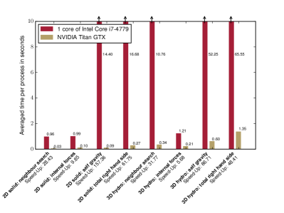
We compared the averaged time per substep for different test cases and particle numbers. Of course, these numbers change with different particle numbers and applications. However, we achieve a tremendous increase in speed for the two most time consuming processes in a SPH simulation including self-gravity: the neighbor search that is used to determine the interaction partners for all particles and the calculation of the gravitational forces with the Barnes-Hut algorithm. These two processes add up to more than 80% of the total computation time. The different subprocesses that are shown in the plot include the following steps: First, the neighbor search determines the interaction partners for all particles. Second, the internal forces calculates all SPH sums and accelerations from the equation of momentum conservation. Third, self-gravity includes all computations that are necessary to determine the gravitational forces between the particles. Fourth, the total right-hand side shows all computations that are necessary to determine the acceleration of all particles.
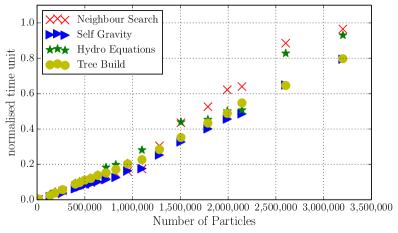
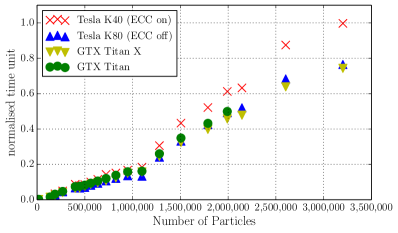
Figure 14 shows the scaling of the code on different GPUs for different number of SPH particles. The time has been normalized to the time used on the NVIDIA Tesla K40 with the device error-correcting code (ECC) enabled. Interestingly, the new consumer devices (Maxwell generation) are as fast as the Kepler generation HPC hardware. However, the consumer GPUs do not provide an ECC mode. The more sophisticated HPC hardware enables the use of ECC for the cost of 20-30% performance. We have not found any differences in the simulation results that would demand the adoption of an automatic error correction code. Since we perform all calculations on the GPU and transfer data to the host only for input/output procedures, the other features of the HPC hardware such as bilateral transfer between host and device are not extensively relevant.
We additionally analyzed the individual scaling for each subprocess of the numerical scheme. Fig. 13 shows the scaling on the NVIDIA Tesla K40 for different number of SPH particles for the simulation of the collapse of the molecular cloud. The scheme for the calculation of the self-gravity of the particle distribution and the scheme for the build of the Barnes-Hut tree show the best scaling.
The increase in speed of the new CUDA version in comparison to our OpenMP implementation is shown in fig. 15. We ran the Prater impact experiment (see sect. 4.3) with both codes for different numbers of SPH particles. The two codes show similar scaling behavior for the number of particles with a constant increase in speed of the GPU version. We intentionally used only one core in the OpenMP version runs for better comparison.
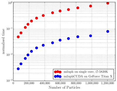
In our first astrophysical application of the code, we were able to increase the resolution by a factor of ten for about equal processing time (see sect. 5.3).
6.3 Numerical limitations
Modern GPUs currently offer fast memory in the range up to 12 Gigabytes (e.g., Tesla K40 and K80, GeForce Titan X) and up to 2880 streaming processors. The size of the memory is the limiting factor for our code. The memory usage strongly depends on the physical model that is applied. Depending on the specific model and dimension, the code holds different information for each particle in the memory. For example, the simplest hydro model only demands information about the location of the particles, their velocities and their masses, that is eight variables in double precision in 3D and only six variables in 2D per particle. For the simulation of solid bodies, the number of variables per particle in the memory increases, since the density, internal energy and deviatoric stress tensor have to be kept available. We additionally store the tree and information about the interactions in the memory. The most expensive model in regard to memory consumption is the damage model, since we need to save the activation thresholds for each individual particle in the memory. Hence, the number of required values per particle grows extensively. The mean number of activation flaws per particle is given by , where denotes the total number of SPH particles. Additionally, the memory demand is related to the choice of the integrator; the Runge-Kutta integrator requires more substeps as the predictor-corrector scheme to store the additional derivatives at the time of the substeps in memory. We allocated about four gigabytes of memory on the Geforce Titan X for the most demanding simulation in regard to memory consumption, the Nakamura experiment in sect. 4.4 with million particles. As can be seen in fig. 12, the most expensive interaction in terms of computation time is self-gravity. The wall clock time of all simulations including self-gravity is dominated by the tree algorithm. For some applications it might be helpful to decouple the hydro timescale from the gravitational timescale, since the code resolves shock waves in the solid bodies while the locations of the particles hardly change. This allows for reusage of already computed pseudo-particles for the calculation of the accelerations due to self-gravity, as long as the tree properties remain unchanged. We added a command line switch for self-gravity simulations that enables this feature. However, we have not used the decoupling for our test simulations presented here.
6.4 Limitations in terms of physical models
As was pointed out by Holsapple (2009), the von Mises yield criterion does not perfectly describe the behavior of geologic materials. The fully damaged material after an impact or a collision should not be treated as a pure fluid, since it behaves more like a granular medium. Hence, the post-impact material flow cannot be modeled realistically with the von Mises criterion. This has already been investigated by Jutzi (2015). To overcome this limitation, we will implement a proper material model for granular media. Another limitation is the lack of a porosity model. Numerous astrophysical objects such as comets and asteroids show high porosities. We would like to apply our newly developed code to simulate collisions between porous objects and plan to include two porosity models to the code: a strain based model (Wünnemann et al., 2006; Collins et al., 2011) and a pressure based model (Jutzi et al., 2008). In the current version of the code, the yield criterion does not depend on the temperature. The change of temperature because of plastic deformation is not calculated. However, these features have been already implemented in the CPU version of the code and will be migrated to the CUDA version soon. This will add more material models to the code, such as the Johnson-Cook plasticity model, where the yield strength depends on temperature and plastic strain and strain rate.
7 Conclusions and future work
We presented a new SPH code for NVIDIA GPUs using the CUDA framework. The code can be applied to various different applications in astrophysics and geophysics. It may be used to model hydrodynamics and solid bodies, including ductile and brittle materials, such as aluminium or basalt. Additionally, the code implements a Barnes-Hut tree that allows for treatment of self-gravity. The code is freely available to the astrophysical and geophysical community upon request by email to the authors.
One main advantage of the CUDA implementation is the enormous increase in speed compared to our existing OpenMP SPH code. The performance of the CUDA code allows for high spatial resolution without the need for cluster hardware. This may enable researchers without access to HPC hardware to perform sophisticated SPH simulations on workstations. Although the code runs faster and more efficient on NVIDIA’s HPC GPUs such as the Kepler GPUs, a large increase in speed compared to the CPU version already exists with the use of cheaper consumer graphics cards. We plan to include more physics in the CUDA version of our SPH code. Currently, we add a porosity model and a more refined plasticity model to the code. One major future step will be to add the support for more than one GPU.
Acknowledgements
We thank the anonymous referee for the thorough review, positive comments, constructive remarks, and
suggestions on the first
manuscript. Christoph Schäfer wants to thank Daniel Thun for various helpful comments about the mysteries of CUDA.
Most plots in this publication have been made by the use of the matplotlib (Hunter, 2007). Thomas Maindl appreciates support by the FWF Austrian Science Fund project S 11603-N16.
Xeon is a trademark from Intel Corporation.
GeForce, Tesla, CUDA are trademarks from NVIDIA Corporation.
longtablell
Glossary of symbols.
\endfirstheadGlossary of symbols continued.
\endhead\endfoot
Parameters for Tillotson EoS
Parameters for artificial viscosity
Crack growth speed
Sound speed
Correction tensor
Dimension
Depth of tree node
Dimension
Parameter for Tillotson EoS
Energy of complete vaporization
Energy of incipient vaporization
Scalar strain
Parameter for artificial stress
Parameter for artificial viscosity
Strain rate tensor
Artificial stress
Gravitational constant
Smoothing length
Second invariant of
Parameter for Weibull distribution
Bulk modulus at zero pressure
Parameter for Weibull distribution
Mass of particle
Shear modulus
Solar mass
Weibull distribution
Parameter for artificial stress
Number of activated flaws
Parameter for Murnaghan EoS
Number of total flaws of a particle
Number of children of a tree node,
Number of total flaws
Number of threads on GPU
Number of SPH particles
Pressure
Artificial pressure for particle and
Distance between particle and
Initial radius of cloud sphere
Rotation rate tensor
Density
Initial density
Parameter for kernel function
Edge length of root node
Edge length of node of depth
Deviatoric stress tensor
Stress tensor
Time
Free-fall time
Temperature
Parameter for Barnes-Hut tree
Internal Energy
Escape velocity
Kernel function
Coordinates of particle
Factor for XSPH algorithm
Velocity of particle
Von Mises yield stress
Angular velocity
References
- Abramowitz & Stegun (1964) Abramowitz, M. & Stegun, I. 1964, Handbook of Mathematical Functions: With Formulas, Graphs, and Mathematical Tables, Applied mathematics series (Dover Publications)
- Barnes & Hut (1986) Barnes, J. & Hut, P. 1986, Nature, 324, 446
- Barnes & Hut (1989) Barnes, J. E. & Hut, P. 1989, ApJS, 70, 389
- Bate & Burkert (1997) Bate, M. R. & Burkert, A. 1997, MNRAS, 288, 1060
- Bédorf et al. (2012) Bédorf, J., Gaburov, E., & Portegies Zwart, S. 2012, Journal of Computational Physics, 231, 2825
- Benz (1990) Benz, W. 1990, in Numerical Modelling of Nonlinear Stellar Pulsations Problems and Prospects, ed. J. R. Buchler, 269
- Benz & Asphaug (1994) Benz, W. & Asphaug, E. 1994, Icarus, 107, 98
- Benz & Asphaug (1995) Benz, W. & Asphaug, E. 1995, Computer Physics Communications, 87, 253
- Benz & Asphaug (1999) Benz, W. & Asphaug, E. 1999, Icarus, 142, 5
- Boss & Bodenheimer (1979) Boss, A. P. & Bodenheimer, P. 1979, ApJ, 234, 289
- Burtscher (2011) Burtscher, M. 2011, GPU Computing Gems Emerald Edition, ed. W. Hwu
- Butcher (1987) Butcher, J. C. 1987, The Numerical Analysis of Ordinary Differential Equations: Runge-Kutta and General Linear Methods (New York, NY, USA: Wiley-Interscience)
- Canup et al. (2013) Canup, R. M., Barr, A. C., & Crawford, D. A. 2013, Icarus, 222, 200
- Collins et al. (2011) Collins, G., Melosh, H., & Wünnemann, K. 2011, International Journal of Impact Engineering, 38, 434
- Dvorak et al. (2012) Dvorak, R., Eggl, S., Süli, Á., et al. 2012, in American Institute of Physics Conference Series, Vol. 1468, American Institute of Physics Conference Series, ed. M. Robnik & V. G. Romanovski, 137–147
- Elbeshausen et al. (2009) Elbeshausen, D., Wünnemann, K., & Collins, G. S. 2009, Icarus, 204, 716
- Gingold & Monaghan (1977) Gingold, R. A. & Monaghan, J. J. 1977, MNRAS, 181, 375
- Grady & Kipp (1980) Grady, D. E. & Kipp, M. E. 1980, Int. J. Rock Mech. Min. Sci. Geomech. Abstr., 17, 147
- Gray et al. (2001) Gray, J. P., Monaghan, J. J., & Swift, R. P. 2001, Comp. Methods Appl. Mech. Engrg., 190, 6641
- Haghighipour & Raymond (2007) Haghighipour, N. & Raymond, S. N. 2007, ApJ, 666, 436
- Hernquist & Katz (1989) Hernquist, L. & Katz, N. 1989, ApJS, 70, 419
- Holsapple (2009) Holsapple, K. A. 2009, Planet. Space Sci., 57, 127
- Hunter (2007) Hunter, J. D. 2007, Computing In Science & Engineering, 9, 90
- Izidoro et al. (2013) Izidoro, A., de Souza Torres, K., Winter, O. C., & Haghighipour, N. 2013, ApJ, 767, 54
- Jutzi (2015) Jutzi, M. 2015, Planet. Space Sci., 107, 3
- Jutzi et al. (2008) Jutzi, M., Benz, W., & Michel, P. 2008, Icarus, 198, 242
- Kulikov (2014) Kulikov, I. 2014, ApJS, 214, 12
- Lange et al. (1984) Lange, M. A., Ahrens, T. J., & Boslough, M. B. 1984, Icarus, 58, 383
- Leinhardt & Stewart (2012) Leinhardt, Z. M. & Stewart, S. T. 2012, ApJ, 745, 79
- Libersky & Petschek (1991) Libersky, L. D. & Petschek, A. 1991, in Lecture Notes in Physics, Vol. 395, Advances in the Free-Lagrange Method Including Contributions on Adaptive Gridding and the Smooth Particle Hydrodynamics Method, ed. H. Trease, M. Fritts, & W. Crowley, 248–257
- Libersky et al. (1997) Libersky, L. D., Randles, P. W., Carney, T. C., & Dickinson, D. L. 1997, Int. J. Impact Eng., 20, 525
- Lindner (2015) Lindner, M. 2015, libconfig@ONLINE
- Lucy (1977) Lucy, L. B. 1977, Astron. Journal, 82, 10134
- Maindl et al. (2014) Maindl, T. I., Dvorak, R., Schäfer, C., & Speith, R. 2014, in IAU Symposium, Vol. 310, IAU Symposium, 138–141
- Maindl et al. (2013) Maindl, T. I., Schäfer, C., Speith, R., et al. 2013, Astronomische Nachrichten, 334, 996
- Marcus et al. (2010) Marcus, R. A., Sasselov, D., Stewart, S. T., & Hernquist, L. 2010, ApJ, 719, L45
- McGlaun et al. (1990) McGlaun, J., Thompson, S., & Elrick, M. 1990, International Journal of Impact Engineering, 10, 351
- Melosh (1996) Melosh, H. 1996, Impact Cratering: A Geologic Process, Oxford monographs on geology and geophysics (Oxford University Press)
- Melosh & Ryan (1997) Melosh, H. J. & Ryan, E. V. 1997, Icarus, 129, 562
- Monaghan & Lattanzio (1985) Monaghan, J. & Lattanzio, J. 1985, A&A, 149, 135
- Monaghan (1989) Monaghan, J. J. 1989, Journal of Computational Physics, 82, 1
- Monaghan (1992) Monaghan, J. J. 1992, ARA&A, 30, 543
- Monaghan (2000) Monaghan, J. J. 2000, Journal of Computational Physics, 159, 290
- Monaghan & Gingold (1983) Monaghan, J. J. & Gingold, R. A. 1983, Journal of Computational Physics, 52, 374
- Nakamura & Fujiwara (1991) Nakamura, A. & Fujiwara, A. 1991, Icarus, 92, 132
- Nakamura et al. (2007) Nakamura, A. M., Michel, P., & Setoh, M. 2007, Journal of Geophysical Research (Planets), 112, 2001
- Pierazzo et al. (2008) Pierazzo, E., Artemieva, N., Asphaug, E., et al. 2008, Meteoritics and Planetary Science, 43, 1917
- Prater (1970) Prater, R. 1970, Hypervelocity Impact: Material Strength Effects on Crater Formation and Shock Propagation in Three Aluminum Alloys (Air Force Institute of Technology.)
- Randles & Libersky (1996) Randles, P. W. & Libersky, L. D. 1996, Comp. Methods Appl. Mech. Engrg., 139, 375
- Raymond et al. (2004) Raymond, S. N., Quinn, T., & Lunine, J. I. 2004, Icarus, 168, 1
- Schäfer et al. (2007) Schäfer, C., Speith, R., & Kley, W. 2007, A&A, 470, 733
- Speith (1998) Speith, R. 1998, PhD thesis, Eberhard-Karls Universität Tübingen
- Springel (2005) Springel, V. 2005, MNRAS, 364, 1105
- Swegle (1992) Swegle, J. W. 1992, Memo, Sandia National Laboratory
- Tillotson (1962) Tillotson, J. H. 1962, Metallic Equations of State for Hypervelocity Impact, Tech. Rep. General Atomic Report GA-3216, General Dynamics, San Diego, CA
- Tingxing et al. (2014) Tingxing, D., Dobrev, V., Kolev, T., et al. 2014, in Parallel and Distributed Processing Symposium, IEEE 28th International
- von Mises (1913) von Mises, R. 1913, Göttin. Nachr. Math. Phys., 1, 582
- Weibull (1939) Weibull, W. A. 1939, Ingvetensk. Akad. Handl., 151, 5
- Wünnemann et al. (2006) Wünnemann, K., Collins, G. S., & Melosh, H. J. 2006, Icarus, 180, 514