A critical reassessment of particle Dark Matter limits from dwarf satellites
Abstract
Dwarf satellite galaxies are ideal laboratories for identifying particle Dark Matter signals. When setting limits on particle Dark Matter properties from null searches, it becomes however crucial the level at which the Dark Matter density profile within these systems is constrained by observations. In the limit in which the spherical Jeans equation is assumed to be valid for a given tracer stellar population, we study the solution of this equation having the Dark Matter mass profile as an output rather than as a trial parametric input. Within our new formulation, we address to what level dwarf spheroidal galaxies feature a reliable mass estimator. We assess then possible extrapolation of the density profiles in the inner regions and – keeping explicit the dependence on the orbital anisotropy profile of the tracer population – we derive general trends on the line-of-sight integral of the density profile squared, a quantity commonly dubbed -factor and crucial to estimate fluxes from prompt Dark Matter pair annihilations.
Taking Ursa Minor as a study case among Milky Way satellites, we perform Bayesian inference using the available kinematical data for this galaxy. Contrary to all previous studies, we avoid marginalization over quantities poorly constrained by observations or by theoretical arguments. We find minimal -factors to be about 2 to 4 times smaller than commonly quoted estimates, approximately relaxing by the same amount the limit on Dark Matter pair annihilation cross section from gamma-ray surveys of Ursa Minor. At the same time, if one goes back to a fixed trial parametric form for the density, e.g. using a NFW or Burkert profile, we show that the minimal can hardly be reduced by more than a factor of 1.5.
1 Introduction
The dwarf spheroidal satellites (dSphs) of the Milky Way are a prime target for Dark Matter (DM) indirect detection searches [1, 2]. First of all, they are relatively close to us and have fairly large DM densities [3, 4, 5], and hence are expected to be among the brightest DM-induced emission. From the point of view of background contaminants, they seem to be ideal objects as well: Intrinsic emission from standard astrophysical sources can generally be neglected (they host old low-luminosity stellar populations and tiny – most often below detection sensitivities – amounts of gas [6]); at the same time, most dwarfs are located at intermediate or high galactic latitudes where Galactic foregrounds are suppressed. Multi-wavelength campaigns have therefore been promoted to search for DM signals, with some of the most impressive results obtained with -ray telescopes: e.g., the Fermi collaboration has recently published updated limits on weakly interacting massive particles (WIMPs), excluding pair annihilating cross sections at the level of WIMP thermal relic cross sections for DM masses lighter than about 100 GeV [7, 8]. Limits from these searches can be meaningfully translated into Particle Physics constraints (see e.g. [9, 10, 11]). Moreover, the compelling DM content of dwarf spheroidals has also triggered general interest from the community in order to assess the nature of the DM particle (see for example the pioneer work in [12] and the more recent [13, 14] and [15, 16]).
A few of the proposed signals (including the -ray flux from WIMP pair annihilations just mentioned or, e.g., the X-ray signal from sterile neutrino decays [17]) are connected to prompt emission from DM particles [18]. In these cases the flux predictions can be conveniently factorized into a term depending on the DM particle physics embedding (specifying, e.g., for a WIMP: the mass, the annihilation cross section and the emission yields), and a term depending on the distribution of DM in the dwarf. For DM pair annihilation signals, the latter – usually dubbed -factor – is defined as an angular and line-of-sight (l.o.s.) integral of the square of the DM density profile:
| (1.1) |
The tight constraints on particle DM properties claimed from dwarf surveys reflect the assumption that fairly small observational and theoretical uncertainties affect these astrophysical factors: e.g. in the analysis of [7] mentioned above, limits are derived exploiting the full ensemble of known dwarfs and introducing a likelihood in which the -factor dependence for each dwarf follows a log-normal distribution of given central value and width . For most of the so-called classical dwarfs – namely the only 8 dwarfs known before the first discoveries of ultra-faint ones as a byproduct in large scale structure surveys [19] – the assumed values of are of the order of 0.2 [20, 21, 7]. This translates into an uncertainty on of about a factor of 1.5. At a superficial level, looking at Eq. (1.1) and assuming as known the distance of the object as well as – most crucially – the shape of the DM density profile, one would deduce that the normalization of the density profile can be inferred from observations with an uncertainty at the 20-25% level.
Indeed, once a specific approach has been adopted in determining such normalization, it is in general true that, in case of the classical dwarfs, the quality of kinematical data is adequate to provide fairly small statistical errors [22]. On the other hand, it is a much more delicate issue to address intrinsic systematic errors of the theoretical models and their impact on parameter determinations, including the normalization and more critically the -factor itself. Analyses in the literature give contradictory results: e.g. [23] presents a comprehensive discussion of the impact of different theoretical assumptions on interpreting kinematical data within the framework of the Jeans equation (a moment projection of the collision-less Boltzmann equation) in the spherical symmetric limit; they conclude that systematic biases and uncertainties on the -factor for classical dwarfs are up to a factor of 3 to 4, including a rather mild impact of a factor of 2.5 from the effect of the dwarf being a triaxial system rather than a spherical one. On the other hand, the authors in [24] (see also Ref. [25]) show that the impact of axisymmetric models for non-spherical DM structures can be much more dramatic on the mass at a reference radius, and hence the normalization of the profile, yielding uncertainties of factors as large as 10 even for the classical dwarfs (Ref. [24] does not discuss the impact on the -factors, but, roughly speaking, the scaling should go as the square of the normalization of the profile).
In this work, while still assuming as theoretical playground the Jeans equation for a spherically symmetric system, we aim to discuss the impact of the method that has been adopted in its solution by the vast majority of recent analyses. This goes into two steps: The first is to introduce parametric forms for the quantities appearing in the equation, namely the DM mass profile and the number density and velocity anisotropy profiles of the stellar populations used as dynamical tracers; The second is to sample the relative parameter space via Monte Carlo techniques in order to perform Bayesian inference, despite some loose theoretical and observational guidance. In particular, it is well known that the stellar anisotropy profile introduces patterns of degeneracies in the result and is unfortunately scarcely constrained by observations. Several recent studies seem to indicate a minor impact on the -factor estimates [26, 27, 28, 29, 22, 30, 31, 32], however they mostly refer to blind analyses involving a marginalization over a parameter space and integration measure which, not being driven by observations or by theory, are essentially an arbitrary choice.
We propose here instead to examine the problem under a different perspective, exploiting an approach in which the Jeans equation is so-to-speak “inverted”, rewriting the DM mass profile in a form in which its dependence on the stellar anisotropy profile becomes explicit. This method was originally outlined in two parallel analyses, see [33, 34]. In this work we re-derive the inversion formula in a new compact form, suitable for numerical analyses, and use it for the first time to discuss -factor estimates. After showing some general trends, we examine, as study case, Ursa Minor, the closest among the classical dwarfs and hence one of those entering critically in the limits concerning the DM particle properties. Results for the -factor are given without the need to marginalize over unknown parameters.
2 Mass models from the spherical Jeans equation
Mass models for dwarf satellites of the Milky Way are most commonly derived exploiting a stellar population as a dynamical tracer of the underlying gravitational potential well (and hence of the dominant mass component, namely the DM mass profile). Supposing that the tracers belong to a non-rotating pressure-supported population in dynamical equilibrium, one can assume that the stellar density function obeys a time-independent collision-less Boltzmann equation, to be solved projecting out velocity moments. Going to the limit in which the stellar and DM components are spherically symmetric, the second moment projection reduces to a single Jeans equation [35, 36], usually recast in the form:
| (2.1) |
This equation shows that the radial dynamical pressure , the product of the tracer number density profile and the radial component of the velocity dispersion tensor , can be expressed in function of itself, as well as of the total mass profile and the orbital velocity dispersion anisotropy . The latter involves also the other two diagonal components of the velocity dispersion tensor and , being defined as:
| (2.2) |
parametrizes the deviation of the velocity ellipsoid from a sphere of radius squared [36, 37]. By definition, can cover the range , where the lower (upper) extreme corresponds to tracers moving on purely circular (radial) orbits. The formal solution of Eq. (2.1) is:
| (2.3) |
The difficulty in fully exploiting this approach is that, despite the assumption of dynamical equilibrium and spherical symmetry at the bases of Eq. (2.1), the problem still involves three unknown functions: , and , to be inferred from only two quantities connected to observations: The first is the stellar surface density:
| (2.4) |
(here and everywhere in the following “” refers to the l.o.s. projected radius, while “” is the radius in the spherical coordinate system centered on the dwarf) which, assuming constant stellar luminosity over the whole system, is proportional to the surface brightness as mapped in photometric surveys (see, e.g., [38]). The second quantity one can derive from observations is the l.o.s. velocity dispersion , which traces the only velocity component accessible to spectroscopic measurements [4, 5]. The l.o.s. velocity dispersion profile can be expressed in terms of the radial dynamical pressure [39]:
| (2.5) |
The mapping of the three unknowns into two observables is usually done by introducing parametric forms for the three unknowns: The template for is typically related to a supported in stellar photometric studies, such as the Plummer [40], the King [41] and the Sersic [42] profiles. usually stems from DM density profile motivated by:
- -
- -
Finally for what regards the stellar anisotropy profile , templates assumed in the literature (see e.g. [48, 49, 50]) reflect more simplicity arguments rather than profound physical motivations, ranging from some constant value to functions connecting two asymptotic values at large and small radii, eventually with some parameter setting the sharpness of the transition.
Attempts to break the degeneracy in Eq. (2.1) between and using higher velocity moments [51, 3, 52, 53, 54, 55] or the determination of multiple tracer populations [56, 57, 58], together with the progress of N-body simulations [59, 60, 61], may represent a promising future opportunity to fully overcome current study limitations due to the l.o.s. measurements available for these systems [62]. Given the large parameter space at hand, one needs an efficient scanning technique and careful addressing of error propagation: For (or directly for )) a frequentist fit of data is usually implemented, in case of the classical dwarfs most often referring to the data compilation in [38]. On the other hand, all recent analyses explore the parameter space connected to and introducing a likelihood addressing the matching of the theoretical model for with data, and employ a Markov Chain Monte Carlo (MCMC) sampling in the context of Bayesian inference. After a choice of priors and integration measures – which in case of the anisotropy function, as for the choice of the functional form, seem essentially arbitrary – one derives posteriors for the parameters defining or , as well as for derived quantities such as the -factor introduced in Eq. (1.1) above. While this procedure gives for the classical dwarfs posteriors on with small error bars, it is not transparent what is the impact of having selected given parametric forms, priors and integration measures, especially in the case of for which a robust physical guidance is still missing. This is one of the issues we wish to investigate in this paper, exploring an alternative approach in which is a derived quantity and the dependance of the result on the assumed form for is kept explicit.
3 General trends from an inversion formula
The method we build on here has been already outlined in two parallel analyses, see [33, 34]. The starting point relies on the observation that the two available observables, namely Eqs. (2.4) and (2.5) above, correspond to the Abel transform of a function :
| (3.1) |
In fact, looking back at Eq. (2.4) the surface density is the Abel transform of the number density profile (everywhere in the following we will use to indicate the number density profile instead of ). In a similar fashion, introducing the projected dynamical pressure, , this expression can be manipulated (see Appendix A for a detailed derivation) inverting it into a formula for the radial dynamical pressure:
| (3.2) |
where is the inverse Abel transform of and we defined:
| (3.3) |
Inserting this result into the Jeans equation [36], Eq. (2.1), one can find the mass profile:
| (3.4) |
with
| (3.5) |
An expression equivalent to Eq. (3.4) can be extracted from Ref. [34], while Ref. [33] gives explicit formulas for several simple anisotropy models; it is however the first time such a compact form in terms of observables is given, showing that the mass profile depends on the anisotropy profile only through the function as defined above. The expression in Eq.f(3.5) shows that, at given , the mass profile can be properly reconstructed if the projected dynamical pressure can be efficiently constrained from data. From the expression just derived one can read out the behaviour of the mass function in some special limits that will be useful in the discussion below. First of all, in case of isotropic stellar orbits, namely for any (and hence ):
| (3.6) |
For circular orbits instead, i.e. for any (and hence , ):
| (3.7) |
Eq. (3.4) is derived under the hypothesis . To take the exact radial orbit limit it is simpler to notice that the radial pressure for (i.e. ) takes the form:
| (3.8) |
and replacing this into the Jeans equation, Eq. (2.1), one finds:
| (3.9) |
3.1 A mass estimator for dwarf galaxies?
As first noticed in MCMC analyses, regardless of what is assumed for the stellar velocity anisotropy , all models fitting the l.o.s. velocity dispersion profile tend to have approximately the same mass at a scale corresponding to about the surface brightness half-light radius [63, 64, 65, 66, 67, 68, 69, 70]. In Ref. [34] a rationale for the existence of such a mass estimator is provided through an analytic manipulation of the solution of the Jeans equation. Briefly recapping their argument, it is useful to consider the difference between the mass profile for a generic anisotropy profile and ; after some algebra one finds:
| (3.10) |
Among the terms within brackets on the r.h.s., towards the outskirts of the dwarf, the logarithmic derivative of the stellar number density rapidly varies from close to zero to a negative number. In the same region, the l.o.s. velocity dispersion is generally close to being flat and also is arguably not too rapidly varying. If one now assumes that also does not have a sharp change in that region, the difference in Eq. (3.10) is approximately zero at the radius defined as:
| (3.11) |
Since this condition does not depend on , almost matches at regardless of the stellar anisotropy:
| (3.12) |
where in the second step the symbol stands for a weighted average on the stellar number density, and has been factorized out in computing and implementing it in Eq. (3.6).
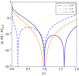
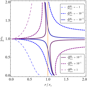
We can check here this result with the formulas derived at the beginning of this Section. We start from a simple model where is assumed to be just a constant , and the stellar profile is described by a Plummer model [40], a case in which the Abel transform can be performed analytically:
| (3.13) |
Under these two working hypotheses, the mass profile in the isotropic case has also a simple analytical form:
| (3.14) |
while Eq. (3.11) gives . Assuming also a constant anisotropy profile, , in the left panel of Fig. 1 we show the relative difference in mass versus the quantity , useful to have circular and radial stellar anisotropies equally spaced in the segment (i.e. corresponds to radial, to isotropic and to circular orbits). The solid orange line corresponds to and shows that in the specific simple model under consideration the goodness of and as mass estimator is within a level of about going to circular orbits, while it degrades to and larger towards radial orbits (in the purely radial limit derived in Eq. (3.9) the discrepancy reaches the value of ). Also shown in the plot is the relative mass difference at and for which there is a better match, respectively, in the radial and circular regimes, as well as a larger discrepancy in the opposite regimes. In the right panel of Fig. 1 we show the isolevels for fixed relative mass difference in the plane versus ; one can see that – still in the same model introduced above – the mass difference is minimized along a curve that is slightly tilted with respect to the estimator proposed in Eq. (3.12), . On the other hand moving away from the match rapidly diminishes in one of the two regimes; for example, taking as estimator radius is in our example a significantly worse choice, with relative mass differences at the level of for purely circular orbits and raising up to the level of 150% in the radial regime. The D half-light radius proposed in [34], namely for the Plummer case, is a better choice.
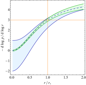
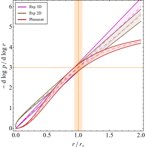
The failure of as an exact estimator stems from the fact that even assuming that is constant, for there is still a non-negligible radial dependence in (for one trivially gets ). This is shown in Fig. 2 where we plot the logarithmic derivative of the radial dynamical pressure versus . This quantity is related to via:
| (3.15) |
and hence, for and constant , it coincides with the logarithmic derivative of the stellar number density . In Fig. 2 is plotted with a dashed line; by definition it crosses the value of at . The blue band on the left panel shows the span in the logarithmic derivative for when varying in the whole range of (respectively, upper and lower boundary of the band). The intersection of the band with the horizontal line at the value of gives the shift on needed to get ; the one with the vertical line at gives instead the magnitude of the departure of from being an exact mass estimator. Although the assumptions in the model we considered may appear rather drastic, the trends displayed are actually general. First, the hypothesis of constant is not critical. Taking into account that available kinematical informations (see, for example, the binned data in [67]) suggest l.o.s. velocity dispersions to be nearly flat in the region around , we can parametrize via the linear expression and vary the slope in a generous range encompassing trends usually reported in literature, as e.g. those in [67] (note however that the error associated to an overall normalization, while propagating on , does not enter in relative mass differences). As can be seen in the left panel of Fig. 2 the impact of this uncertainty is marginal with respect to the one due to the orbital anisotropy. The same conclusion holds when considering also the second ingredient at hand, the modeling of the stellar distribution. As alternatives to the Plummer model, we introduce the two following exponential templates:
| (3.16) |
for which , and:
| (3.17) |
for which ( is the modified Bessel function of the second kind). The functions above qualitatively reproduce typical realizations of a multi-parameter template like the Sersic profile, while differing substantially in the inner region from the Plummer model (the King model is instead qualitatively equivalent to the Plummer). Back to the working hypothesis of constant and , we plot in the right panel of Fig. 2 the logarithmic derivative of as a function of for the three stellar profiles. The uncertainty bands displayed are obtained by the generation of a set of surface brightness mock data with binning and associated errors matching typical photometric maps of the 8 classical dSphs as in [38]. Although within a given stellar profile the impact on from our estimated uncertainty on is negligible as shown in Fig. 2, a higher impact derives from the mis-reconstruction of the stellar profile within a wrongly assumed parametric form, see the shift in with respect to the observable radius between the Plummer model and the two exponential profiles.
To summarize this part of the discussion, we find that the uncertainty on the dwarf mass estimator is dominated by the kinematical determination of the normalization on as long as models with radial-like tracer orbits are not included in the analysis. While general criteria hinting for unphysical phase-space densities in connection to radial-like tracer orbits are present in literature (see e.g. [71, 72]), a rigorous theorem for the exclusion of these scenarios holds only at the center of the system [73].
3.2 Extrapolating to inner radii: densities profiles
While in the standard approach to solve the Jeans equation, Eq. (2.1), physical mass profiles are automatically obtained imposing a “physical” parametric ansatz, there is no a priori guarantee that the procedure proposed here gives physical outputs.
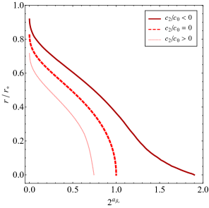
A first basic check is on the positivity of the solution of Eq. (3.4) at any radius. E.g. in the simplified model introduced above one finds a non-trivial constraint on the allowed range of orbital anisotropies. This is shown in Fig. 3 in the plane -, where isolevels for are displaced in the limit of constant orbital anisotropy, marking the minimum radius at which a solution of Eq. (3.4) is positive. In particular, the red dashed line corresponds to the case of constant and Plummer surface brightness. One can see that, within this setup, positive mass solutions can be extrapolated down to only when . On the other hand, the extrapolation to critically depends on what is assumed for the extrapolation of for . To sketch this effect we introduce as sample parametrization for the l.o.s. velocity dispersion the form: iff , constant iff . Fig. 3 shows that an inner concave tilt of forces to restrain to progressively more negative values of (with approaching 1), while a concave one allows for radially anisotropic stellar velocity profiles.
In general, the positivity of the mass is not the only condition we would like to supplement the Jeans inversion with: e.g. the mass profile should not decrease going to larger radii (i.e., up to the cutoff of the profile). In the following, we will be actually more restrictive and define as a physical outcome of our inversion the model satisfying the following requirements:
| (3.18) |
Assuming that the density of the DM profile provides the dominant component to the dSph potential well, the third condition ensures the potential well to be monotonic and hence provides a necessary condition of stability for the model.
Checking a posteriori these conditions, is simply obtained taking the derivative of the mass function, Eq. (3.4):
| (3.19) | |||||
Among the three terms on the r.h.s., only the first contributes in the limit of isotropic motion of the tracers ( or equivalently ); assuming also that the l.o.s. velocity dispersion is constant, one simply finds:
| (3.20) |
For such profile to have a core (namely: for ), the logarithmic slope of the stellar density profile needs to scale as towards the center of the system. E.g., considering a multi-parameter stellar template like the Zhao profile [74]:
| (3.21) |
where and represent the inner and outer slope of the profile, and and the scale radius and the smoothness of the transition between the inner and outer scaling, the logarithmic slope is:
| (3.22) |
and a cored profile is obtained only in case and . For any the scaling of the DM profiles jumps to , as in the isothermal sphere model.
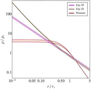
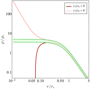
Looking back at Eq. (3.13), one sees that the Plummer model belongs exactly to the class of the Zhao profiles providing a core in if is constant. This is also shown in the left panel of Fig. 4, where we plot the result for the inversion within the assumptions of constant and . In the same plot we show also the resulting case of the two exponential stellar templates introduced in Eq.(3.16)-(3.17). Note that an exponential surface brightness implies a logarithmically divergent stellar number density and hence a scaling of the inner density of , while the (cored) exponential stellar density gives a inner density scaling, standing in between the cored case and singular isothermal sphere. Indeed, the Plummer model is the simplest stellar template we can consider which provides a core in the density profile. Since cored profiles are of particular importance when estimating minimal values for the l.o.s. integral of squared densities (the -factor defined in the Introduction), it is the case we will concentrate on in the following.
Before discussing the case of , it is interesting to assess how the density profile is affected by a mild departure from the approximation of constant . The green band in the right panel of Fig. 4 shows the very mild impact on when we implement the linear scaling of the l.o.s. velocity dispersion already introduced in Fig. 2. For the quadratic scalings already implemented in Fig. 4 – even using much milder concave and convex tilts for – one sees instead a rather drastic change in , with a sharp enhancement of the inner density for a convex perturbation and an unphysical solution induced by the concave tilt. Associating the trends seen in the left and right panels of the figure, one can deduce that a cored profile, standing also at the border with unphysical solutions, is obtained in the inversion procedure only via a fine adjustment between the trend imposed by the choice of stellar number density profile and that from the scaling of .
We are now in the position to address the implications on of a non-vanishing orbital anisotropy, considering first of all the case in which it does not depend on the radial coordinate, i.e. . Looking back at Eq. (3.19), also the second and the third term on the r.h.s. give a contribution to ; the second term however has the same scaling as the first, hence does not alter the discussion just presented for . The third term instead introduces a non-trivial dependence on of the inner radial slope. Assuming , the scaling can be read out from the corresponding logarithmic derivative diminished by 2 (taking into account the factorized on the l.h.s. of Eq. (3.19)):
| (3.23) |
In general the term is the most relevant, driving to a scaling that is even more singular than the singular isothermal sphere in case of circularly anisotropic profiles; the term in the logarithmic derivative of can at most mitigate the singularity in case itself is singular. The last term on the r.h.s. of Eq. (3.23) is in general less relevant; for constant and a Plummer , in the limit it is equal to 0 if , and to for . In this last case, one would apparently get a cored profile; note however that is obtained by summing this contribution to the first two terms in Eq. (3.19), and, in the same limit, these drive to an unphysical result, with the negative mass solution already discussed above. Analogously to what is shown in Fig. 4, a proper readjustment of the inner radial scaling of would be needed, requiring however a even more severe tuning to get physical solutions with a core [75], since impacts also on the scaling in Eq. (3.23).
A further subtle point regards the limit of . When approaches extreme negative values, the logarithmic derivative of appears as an extra multiplicative factor in the third term on the r.h.s. of Eq. (3.19) and hence its radial scaling (the logarithmic derivative of the logarithmic derivative of ) should be added to Eq. (3.23). Referring again to the Zhao profile in Eq. (3.22), this contribution is 0 if , it is equal to if . Back to the Plummer model and constant one would then find a scaling of the density profile that goes like , as opposed to valid for .
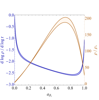
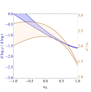
In the left panel of Fig. 5 we show the slope of the density at the fixed value as a function of all the set of that provide a physical solution (see Eq. (3.18)) in our Jeans inversion approach. The resulting blue band in the plot highlights qualitatively the trend analyzed so far: Exploring even smaller ratios of , one would retrieve the linear scaling with sudden transition of to at and to at .
Once we leave the center of the dSph to move towards its outskirts, such a behaviour related to the allowed physical solutions gets relaxed: e.g. at , within the uncertainty of the Plummer profile, physical densities are allowed up to , scaling with a power law index between and , as represented by the blue band in the right panel of Fig. 5.
Also shown in the same figure is the value of the profile at the two chosen radii normalized to . In the central region of the system there is a smooth, but sharp, variation of the density varying , spanning roughly two orders of magnitude. On the other hand, at large radii the variation in is within .
The subtle limit could have been inferred also looking at the behaviour of the mass profile in the case of purely circular stellar motion. In fact, for the model implementing a constant and Plummer surface brightness Eq. (3.7) goes as:
| (3.24) |
and in the limit of going to 0 becomes
| (3.25) |
We observe that the case of constant orbital anisotropy going to is the only case when the condition of is not met in this model, mimicking the scenario of a black hole at the center of the dwarf supporting the velocity dispersion. With the logarithmic slope of approaching , the mass profile gets larger and larger contribution close to . The logarithmic divergence is avoided via the appearance of the black hole-like feature and hence a discontinuity in the density profile:
| (3.26) |
holding a logarithmic slope equal to at the center, as anticipated.
We summarize the results of this section, briefly recapping what we have achieved so far with our method. First, we have highlighted the existence of possible unphysical solutions encoded in the general master formula, Eq. (3.4), derived by inverting Eq. (2.1). Physical solution within this approach require the following two conditions:
-
i)
-
ii)
Then, we have made a step forward deriving Eq. (3.19) to study the density of non-rotating pressure-supported systems like dSphs. In order to deal with a physical density, we have supplemented the latter with the following third condition:
-
iii)
We have primarily focussed our attention on the trends of the inner density profile of the system for several tracer density templates and l.o.s. velocity dispersion profiles, see Fig. 4, under the assumption of an isotropic tracer motion. Eventually, we have analyzed in details the benchmark scenario of and stellar Plummer model, varying the orbital anisotropy , as reported in Fig. 5.
3.3 -factor scalings
The simple form of derived in the circular anisotropy limit may be taken as a good starting point to discuss -factor trends in the inversion approach considered here. Indeed, integrating the square of the profile in Eq. (3.26) following the definition in Eq. (1.1), we can get an analytic form for the . In Appendix B we provide an expression for the -factor, see Eq. (B.10), which is valid in the limit of distance of the dwarf much larger with respect to the typical transverse size of these galaxies (note that the optimal angular aperture is usually considered in literature, see e.g. [26, 20, 23]). In the case at hand it gives:
| (3.27) | |||||
where the quantity in the last brackets is an energy density and the dimensionless ratio is introduced to take into account a possible finite size of the spherical halo density .
Plugging in Eq. (3.27) typical values for dSphs, namely km s-1, kpc and kpc, one gets a -factor of about GeV2 cm-5.
Notice that this is not a totally realistic case since the black hole mass one would infer from Eq. (3.25) would be , possibly consistent with kinematical observables, but likely too high to be found at the center of these galaxies [76, 77] .
Even in case of perfect isotropic motion of the stellar tracers an analytic expression for the density profile, Eq. (3.20), and the -factor can be provided. For the latter we have:
| (3.28) |
that is a factor of larger than the case.
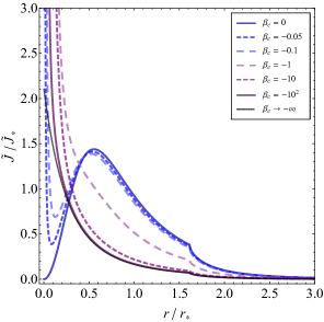
The picture for constant orbital anisotropies related to physical solutions (still taking constant and Plummer profile) is shown in Fig. 6:
we plot a function appearing as a linear measure in the -factor computation (the area under each curve represents the J-factor, up to the normalization factor ), see Eq. (B.9).
Then, the general trend for the -factor at constant can be drawn: Starting from the minimum -value corresponding to the case of , the -factor increases going to smaller values of , with an inner cusp appearing and at the same time a reduction of the contribution at larger radii, up to the exact circular limit, when the central cusp is suddenly reduced in correspondence to the discontinuity of .
As anticipated, the picture above is expected to provide a rather conservative estimate of the -factor: leaving a cored stellar template in favor of a more general Zhao profile, Eq. (3.21), with , or an exponential template, like the Sersic one, would enhance the inner density profile and hence the -value; moreover, an inner convex tilt in the profile of the l.o.s. velocity dispersion would go in the same direction. A concave perturbation to a flat would offer a way out to lower the -value, but would apply only to the cases of circular-like stellar orbits, where the density is relatively cuspy, to not generate unphysical outputs like the one previously encountered in Fig. 4. Therefore, discarding the “extreme” solution of the Jeans inversion at , the lowest -factor emerging from a physical model in Fig. 6 corresponds to the case of perfectly isotropic stellar motion, Eq. (3.28).
Within the same framework, this conclusion can be modified once we follow a more conservative approach in extrapolating the inner density of .
Indeed, one may question whether the basic assumptions involved in the derivation of Eq. (2.1) itself, most importantly the spherical symmetry of the system, should be trusted down to exceedingly small radii, imposing by construction a choice of coordinates which are singular in the origin and also extrapolating in a region which is simply not accessible with data. An alternative is to introduce a saturation scale so that ; in Fig. 6 one sees that a relatively small inner cutoff, i.e. , has an important impact on the inner density profiles with and hence on the corresponding -factors.
Focussing on the area below each curve of Fig. 6 one can easily visualize that in the case of , the -factor is almost insensitive to an inner cutoff,
while for a negative orbital anisotropy, a very small can significantly enhance the -value with respect to what can be obtained with a more conservative cut on the inner density.
In the exact circular orbit limit the -factor is again quite insensitive to the choice of .
Note that with the implementation of , the density related to very negative orbital anisotropies is now smoothly tracking the – previously discontinuous – case of circular orbits. Therefore, the flattening of the density due to the a non-vanishing inner cut allows for lower -factors than the one obtained at .
At the same time, one should not forget that lower orbital anisotropies in this context would imply growing black-hole-like features up to the questionable point that an important contribution to the total mass of the system comes from the center.
Eventually, note that – in contrast to the approach followed in this work – a physical black hole at the center of the dSph may be instead modeled so to strengthen the DM annihilation signal from the galaxy. This possibility has been explored in, e.g., [78, 79].
Focussing on the minimum -value one can obtain, we can now address the impact of a radial dependence in the orbital anisotropy function. In what follows we will assume the orbital anisotropy profile to be well described by the rather general form provided in [50]:
| (3.29) |
offering an interpolation between the tracer behaviour at the center of the system, set by , and the one towards the outer
part, set by , with characteristic scale and sharpness between the two regimes respectively determined by and .
Note that, on general grounds, for solution to be physical satisfying the conditions in Eq. (3.18), a sharp radial dependence in (such that its derivatives would even impact on the scalings discussed looking at Eq. (3.23)) can be implemented only together equally sharp variations of in ; we will provide an explicit example in the next Section, enlightening also the level of tuning involved. Here we will consider instead smoother behaviour for , assuming then, without loss of generality, a constant and referring to the trends illustrated in Fig. 4 for its extensions.
We have seen in Section 3.1 that a notion of a mass estimator for the system is to some extent available thorough the mass enclosed in . We can exploit this information to find the density profile that minimizes the -factor. This can be done introducing a simple broken power-law ansatz for :
| (3.30) |
with being the logarithmic derivative of the profile within the radial interval , the Heaviside step function, and the normalization is derived from the condition . For a given (as following from the approximate relation in Eq. (3.12)), -factor can be minimized as a function of the and .
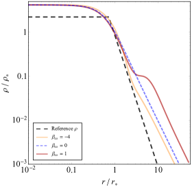
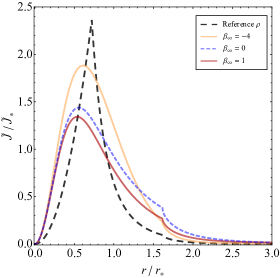
In Fig. 7 we show the outcome of this procedure in the sample case of 4 power laws indices; we imposed as constraints 111Here we are also assuming the mass profile to grow at least logarithmically with the radius, as e.g. for a NFW profile. and : Not too surprisingly the result is that the profile minimizing the -factor at given , drawn with a black dashed line, is cored for and it drops to as fast as possible for larger ; we checked explicitly that such result is independent of number of power laws assumed to model .
This result provides an independent check about our findings at constant orbital anisotropy: as long as the volume integral of the density profile at encloses the whole mass in , i.e. no black-hole-like feature is present, the physical configuration that has the minimum -factor happens to be at , namely when features an inner core.
In Fig. 7 we report with a dashed blue curve the density profile obtained from the Jeans inversion procedure with , constant , Plummer stellar profile and same of the reference density. The good agreement with the latter in the innermost part of the profile does not leave so much room for improvements. Indeed, exploiting the orbital anisotropy form of Eq. (3.29), a good match to the black dashed line requires to generate an inner core. Moreover, one needs to have such a core as extended as in the reference case. Consequently, one ends up to require (but not too large in order to not invalidate conditions in Eq. (3.18)) to get an appreciable departure from isotropy with .
We display this set of results in the left and right panel of Fig. 7:
-
•
In the left panel we show two different configurations of the density profile with in the outskirts of the dSph, through a mildly circular-like or a purely radial value assigned to . Both profiles do not provide a dramatic improvement in matching the reference density.
-
•
In the right panel we see that the -value corresponding to the case of has slightly increased, while the radial case gives slightly lower values of (an effect anyhow at the per mille level). Note however that in the limit of the density is almost turning to an unphysical profile, since an unphysical ripple is starting to appear.
We can then conclude this Section stating that in the search for density profiles that minimize the -factor – within a given mass at the radius , as constrained by kinematical data – a radial dependence in the unknown orbital anisotropy profile does not significantly alter the picture previously outlined assuming constant .
4 The study case of Ursa Minor
4.1 A few generalities on the dwarf
Ursa Minor is most often referred to as the target for which both signal and background are most reliably estimated, providing a very competitive limit on annihilating DM models. As discussed in the first analysis on Milky Way satellites by the Fermi collaboration [20] (assuming NFW DM profiles and a fixed angular acceptance of solid angle sr), and in agreement with previous analyses [1], Draco and Ursa Minor are the prime targets among the classical dSphs. Ref. [80], assuming instead a Burkert profile and performing an optimization of the angular acceptance, discussed uncertainties in the gamma-ray background determination, concluding that Ursa Minor is the favorite target from this point of view, followed by Sextans which however provides less stringent constraints, while large uncertainties lie in Draco and Sculptor.
All this motivated us to consider Ursa Minor as a suitable sample object for the purpose of our study.
We briefly summarize here the main characteristics of this satellite, specifying some of the choices for the data set considered in the phenomenological analysis that follows.
The wide field photometry study in [81] finds that Ursa Minor hosts a predominantly old stellar population, with virtually all the stars formed before
10 Gyr ago, and 90% of them formed before 13 Gyr ago, making it the only dSph Milky Way satellite hosting a pure old stellar population. Using the magnitude
of the horizontal branch stars and comparing with Hipparcos data on globular clusters the authors determined the distance of Ursa Minor from the Sun to be
kpc, in agreement with the determination from [82], but larger than the mid 1980’s value of kpc quoted in
[83, 84]. As pointed out in [85], the difference is mainly due to the absolute magnitude calibration of the horizontal branch;
standing in between are the values of kpc [86] and kpc [87]. Here we choose to adopt the mean value kpc from the old determination of [83, 84], since most often the same has been done in the most recent literature discussing J-factor uncertainties, see, e.g., [32].
Note that, while we will be mostly concerned about relative shifts on J-factor determinations connected to the solution of the Jeans equation, switching from 66 kpc to 76 kpc would imply an overall decrease in values quoted below of about 25%.
Regarding the stellar surface brightness, the one of Ursa Minor shows the largest ellipticity among all classical dwarfs (excluding Sagittarius that is suffering heavy
tidal disruption), with mean value of (where is the minor over major axis ratio) estimated in [38] to be .
Nevertheless, most analyses treat Ursa Minor as a spherically symmetric system, with stellar surface brightness to be fitted with a template,
most often via the Plummer, the King or the Sersic model. We will follow [67, 68] which suggest to adopt the Plummer model, also in view of the discussion on stellar number density profiles in the previous Section. While the value of the normalization parameter in Eq. (3.13) does not need to be specified in the Jeans analysis as well as in its inversion,
as projected half-light radius we assume kpc, estimate originally obtained in [38] from a geometric average of the corresponding half-brightness radii along the semi-major and semi-minor axis of the projected stellar profile.
In what follows, the computation of the l.o.s. integral of of Ursa Minor will always refers to pointing to the center of the system with the optimal angular aperture , as most often adopted in literature (see e.g. [7, 32]). J-factors will be computed according to Eq. (B.8), integrating up to an estimated outer radius kpc (changing this to an arbitrarily larger value, as
a negligible numerical impact, generally at the per mille level).
4.2 Jeans inversion with Ursa Minor data
The starting point of our phenomenological analysis on Ursa Minor is a fit of the binned l.o.s. velocity dispersion data from [67]. We consider two possibilities for the fit: i) The standard approach in which is computed solving the Jeans equation, see Eq. (2.3)-(2.5), for given parametric forms of the DM density and of the orbital anisotropy (in the following we will refer to this procedure as parametric fit); ii) A direct fit of the data within a given functional form for (in the following: -driven fit).
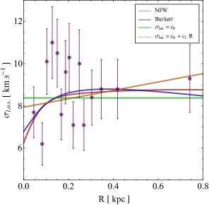
The result of the fit according to four different benchmark cases is shown in Fig. 8. The two parametric fits correspond to a cuspy and a cored , namely a NFW and Burkert halo density together with the assumption of constant orbital anisotropy. The other two cases considered are of the two simplest of the -driven kind, namely constant and a linear regression in . The best-fit parameters and the corresponding are given in Table 1; as it can be seen all the four benchmarks provide fairly good fits and comparable .
| Benchmark | Parameters | Mean value | 68% C.L. | |||||||||||
|---|---|---|---|---|---|---|---|---|---|---|---|---|---|---|
| NFW |
|
|
|
|
||||||||||
| Burkert |
|
|
|
|
||||||||||
|
|
|
|
|||||||||||
|
|
|
|
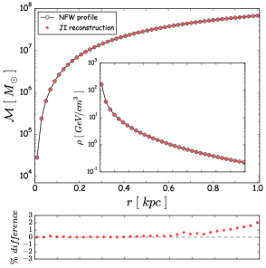
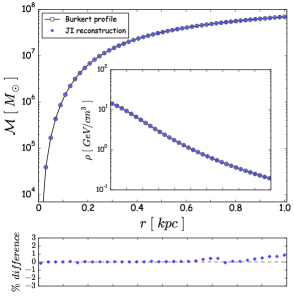
Fits of the l.o.s. velocity dispersion data are taken as an input for the procedure of inversion of the Jeans equation, to reconstruct – at given – the DM mass and density profiles, and hence study how the minimal -factor of Ursa Minor, i.e. the 2 lower-limit of the posterior distribution of , depends on the assumed . The different choices of have been considered to check whether the parametric fit from an a priori physical model and/or the -driven fit (agnostic, but non-necessarily corresponding to a physical model) may be introducing a bias in the analysis. Incidentally, the parametric fits also allow for a cross-check on the accuracy of our numerical implementation of the inversion procedure. In Fig. 9 we show profiles reconstructed via Eq. (3.4) compared against the initial NFW and Burkert parametric forms. The latter are given as an input to derive the parametric fits for , which are displayed in Fig. 8. To perform this exercise we used the best-fit values specified in Table 1. The displayed reconstruction of the mass profile for both cuspy and cored cases comes with a level of accuracy better than the per mille in the whole range of the binned dispersion data of Ursa Minor, i.e. pc; relative differences above few percent arise only at inner radii much smaller than pc. A similar level of accuracy is found for the reconstruction of the inner density profile, for which we also show the relative percentage difference in the insets below the two plots. The density profile of parametric fits can be conveniently evaluated via an iterative difference quotient algorithm [89] applied to the mass profile.
4.3 Inversion and MCMC with constant anisotropies
When investigating the impact of orbital anisotropy on density profiles and -factors the emphasis will be on discussing minimum values consistent with kinematical observables. In fact, since the DM velocity-averaged pair annihilation cross section accessible to gamma-ray observations scales with the measured flux as
| (4.1) |
the lowest -value allowed by Ursa Minor data can be directly linked to how much the upper-bound on , reported e.g. in [21] for this galaxy, can be relaxed. As shown in Section 3, the minimum -value turns out to be weakly affected by a radial dependence of the anisotropy profile as long as is mildly varying in as well. Thus we can restrict our phenomenological analysis to the simple case of without loss of generality in the conclusions.
Starting with the four benchmark cases for shown in Fig. 8, in the left panel of Fig. 10 we show results for as a function of the value assumed for and in the range corresponding to models satisfying the set of conditions for a physical model, see Eq. (3.18): for the parametric fits only values of lower or equal than the one assumed for computing are allowed; for the -driven fits, the Jeans inversion procedure gives physical models up to . Note that the exclusion for all the four benchmarks of constant radial-like anisotropy profiles, matches with the requirement of to obtain a positive stellar phase-space density at the center of the system [73]. The behavior of as a function of is qualitatively the same for all the four scenarios: For a given stellar surface density and when starting from close to 0 and going to progressively larger circular anisotropy the density profiles becomes progressively more concentrated and hence the -factor grows, up to the level one starts to see the turnaround in logarithmic slope already seen the left panel of Fig. 5 when getting close to the pure circular orbit limit. The decrease in -factor at this turning point becomes even more pronounced since we are taking here the conservative view of not extrapolating the profile obtained from the inversion procedure all the way to . We rather introduce a inner density cutoff , with pc as sample value avoiding an extrapolation to radii smaller than the order of magnitude of the radius in the innermost bin of data. The two benchmark obtained from parametric fits are both characterized by a concave inner tilt; this makes the density profile shallower than those for the -driven cases at small negative values of and hence we find lower -factors. On the other hand the same concave tilt partially washes out the cancellation we discussed for purely circular orbits, as well as makes the effect of the internal cutoff less severe, and hence drives a less pronounced decrease of the -factor at very large negative . In the left panel of Fig. 10 we show also the band for the Ursa Minor -factor adopted in the Fermi-LAT analysis of Ref. [7] (scaled to the same dwarf distance adopted here): the minimum -values for the parametric fit cases are obtained for the same implemented to generate the profiles and are within with respect to Fermi quoted values (we take the Fermi band as visual guide only and do not intend to make any statistical statement at this point). For the case of -driven fits, i.e. when assuming a constant or a linear regression, the minimum turns out to correspond to the circular orbit limit; in particular to the sample benchmark with constant the minimum is roughly away from the nominal value in [7] for Ursa Minor, driving – as naive estimate – a relaxation of the extrapolated limit on of a factor of few. On the other hand these correspond to rather extreme configurations, with, as explained in the previous Section, extreme cusps which would be developing in the very inner region of the system (even below the cutoff radius we are considering), finally shrinking to a profile and a central black hole. The black hole mass for would be of the order of or larger, and while it could be physically motivated that to have a flat density around them, see, e.g., scenarios in Ref. [90], such masses are at the edge of observational limit for this system [91, 92].
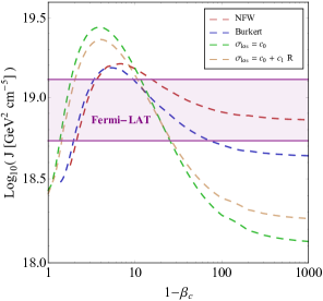
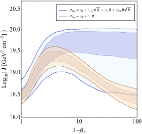
In order to provide a more robust statistical assessment of these findings, we also present here the results of a Bayesian fit of Ursa Minor binned data, computing the -factor through the inversion formula for a finite grid of constant orbital anisotropies. We have exploited for the purpose two different parameterizations of , namely the same linear expression in already introduced, and the following polynomial form (recall that is the outer radius and we picked as reference value 1 kpc):
| (4.2) |
This form has been chosen since it can nicely interpolate among the four benchmarks in Fig. 8 within a broader set of behaviours, including,
eventually convex tilts at small .
To perform our MCMC analysis we use the Bayesian Analysis Toolkit library [93], assigning generous flat priors to the coefficients defining ,
namely , , and , and performing a total of iterations distributed in chains.
In each iteration of the MCMC we invert the Jeans equation for all the set of considered, computing the density profiles via Eq. (3.19) and the -factor when the physical
conditions in Eq. (3.18) are met.
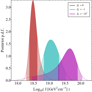
As a result of this involved procedure, we obtain in the end the posterior probability density function of for each of the selected constant anisotropies, i.e.
without any marginalization procedure over unknown parameters unrelated to observable quantities.
| [GeV2 cm-5] | [GeV2 cm-5] | |||||
|---|---|---|---|---|---|---|
|
|
|
|
||||
| Eq. (4.2) |
|
|
|
In the right panel of Fig. 10, we plot the and probability region of for orbital anisotropies in the range , finding again for the linear parametrization of that the minimum value of happens in the circular orbit limit, with precise value sensitive to the choice of inner cutoff radius at pc. While the more general parametrization in Eq. (4.2) encodes the linear behaviour as well, the latter becomes now only a special realization of it, and consequently populate the tail of the distribution in when one probes lower ad lower stellar anisotropies. This trend of the posteriors of is summerized in Fig. 11, where we show three illustrative cases, highlighting with the color code their and probability area (defined from the local mode of the distribution). Eventually, we can conclude that the lowest -value is again found in correspondence to the isotropic stellar motion when considering the case of Eq. (4.2), while it is provided by the limit of circular-like orbits in case a linear form for is implemented (together with the caveats of the related black hole feature discussed above). For what concerns the bounds on the cross section of a DM annihilating pair, in Table 2 we report the naive maximum relaxation one can apply to these limits for the study case of Ursa Minor: We remark that at one can naively relax the Ursa Minor upper-bound on by a factor roughly ranging from 2 to 4.
4.4 -factors and from NFW and Burkert profiles
While the general impact on for spatially dependent orbital anisotropies has been qualitatively discussed in Section 3, we try to address here a slightly different, though related issue: within a physically motivated ansatz for the DM density profile of the system, what is the orbital anisotropy profile compatible with the velocity dispersion data that, at the same time, provides the smallest -factor possible for the galaxy?
Assuming a rather general form for the profile of , we can answer to this question quantitatively taking again Ursa Minor as our study case.
Taking as reference parametric forms the NFW or Burkert profiles, these are completely determined by only two parameters, namely a characteristic scale radius and a normalization . As discussed in Section 3.1, in case of nearly flat projected l.o.s. velocity dispersion profile in the outskirts of galaxy – a condition fulfilled by Ursa Minor, see Fig. 8 – the mass enclosed within the radius (close to the half-light radius of the stellar profile and defined as the radius at which its logarithmic slope is equal to -3, see Eq. (3.11)) is nearly independent of the assumed orbital anisotropy profile. To a good approximation, we can then trade the normalization of the DM profile by :
| (4.3) |
This expression then sets the normalization of to be a function of and , with in turn the latter being set in terms of the normalization of . At fixed , the -factor for the profile becomes only a function of and selecting the minimum fixes this parameter as well, fully determining the density profile. Eventually, assuming a definite form for the stellar anisotropy, one is able to read the profile from a fit of the dispersion data.
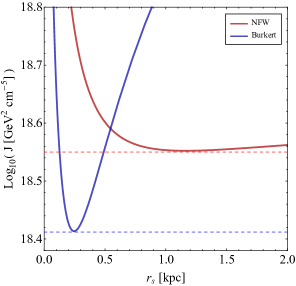
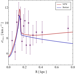
In Fig. 12 we show the logarithm of as a function of the scale radius for both the NFW and Burkert cases fixing , as follows from applying Eq. (3.12) to the Ursa Minor binned data. Analogously to the results in Section 3, for both the NFW and Burkert profiles, the minimum of corresponds to an intermediate value for the scale radius such that the density profile flattens as much as possible in the inner part, and falls off rapidly in the outskirts. Comparing the two cases, the lowest -value corresponds once again to the most cored of the two density profiles. The radius that minimizes at fixed is reported in Table 3. Having selected within this approach one NFW and one Burkert profile, we search for a compatible orbital anisotropy profile through Eq. (2.3)-(2.5), using Ursa Minor velocity dispersions data and the parameter function in Eq. (3.29) for . The corresponding best-fit are plotted in the right panel of Fig. 12 and are generated in both cases by a making, in correspondence to the deep in , a violent transition between a mild circular orbit regime to a purely isotropic tracer motion. The nominal best-fit values of the anisotropy parameters are collected in Table 3, together with the of the fit related only to the stellar anisotropy degrees of freedom.
| [kpc] | [kpc] | |||||||||||||
|---|---|---|---|---|---|---|---|---|---|---|---|---|---|---|
| NFW |
|
|
|
|
|
|
|
|||||||
| Burkert |
|
|
|
|
|
|
|
Since the value of [GeV2 cm-5] for Ursa Minor reported by the Fermi collaboration in [21] is respectively and for an assumed NFW and Burkert density (considering a distance of kpc), according to our findings in Table 3, the minimum possible compatible with a mass estimator of and a NFW or Burkert profile is essentially within the range of the corresponding Fermi-LAT quoted value. An uncertainty to can be naively associated from a simple constant fit of the dispersion data, namely . Then, at we find that the minimum mass estimator is and the corresponding -factor in Table 3 shits to the value of GeV2 cm-5 for the NFW profile, GeV2 cm-5 for the Burkert case. It follows that relaxation of the DM particle physics limits results only in a factor of or , respectively for the cuspy or cored cases. Hence we conclude that, when assuming a definite functional form for the DM density profile, the Fermi-LAT bounds result to be quite robust even against the extreme case of a dramatic radial dependence in the tracer orbital anisotropy.
5 Conclusions
We have considered the spherical Jeans equation for a non-rotating pressure-supported tracer population, and reexamined a method to solve it in which the Dark Matter mass profile – accounting for the underlying potential well – appears as an output rather than a trial parametric input as required in the standard approach. We obtained a very compact form for such explicit expression for the mass profile, showing that it depends just on the derivative of the inverse Abel transform of the radial dynamical pressure, and on the tracer orbital anisotropy profile , to be rewritten in terms of the function . We have exploited this new formulation to discuss, on general grounds, to what level dwarf spheroidal galaxies feature a reliable mass estimator – the total mass enclosed within the radius at which the logarithmic derivative of tracer number density profile is equal to -3 (in the outskirts of the dwarf, at about 1.3 to 1.5 times the half-light radius of the projected surface brightness) – regardless of the assumptions on the (unknown) orbital anisotropy profile. We have then turned to discuss the Dark Matter mass and density profiles in the inner region of the system, enlightening connections with assumptions on the inner scaling of the tracer number density profile and the shape of the tracer line-of-sight projected velocity dispersion. Having kept explicit the dependence on , we have illustrated the induced scalings on the density profile and hence on the angular and line-of-sight integral of the density squared, the quantity usually dubbed -factor and entering the predictions of prompt Dark Matter pair annihilation signals, including the prompt gamma-ray signals the Fermi-LAT instrument has searched for and put constraints on.
We applied the method to one sample case, the Ursa Minor Milky Way satellite. After discussing general trends on a few benchmarks, we have performed a Bayesian fit via an appropriate parametrization of the tracer line-of-sight projected velocity dispersion without involving a marginalization over unknown quantities. We compared -factor at given assumed orbital anisotropy with values quoted in the literature; in particular, the emphasis has been to extract information about minimal -factor compatible with Ursa Minor kinematical data. In this respect we conclude: In a blind analysis, assuming no prior knowledge of the Dark Matter density profile, minimal -factor can be a factor of 2 to 4 smaller than commonly quoted estimates, relaxing by the same amount the limit on Dark Matter pair annihilation cross section deduced from gamma-ray surveys of Ursa Minor. At the same time if one goes back to a fixed trial parametric form for the density profile, such as the NFW or Burkert profiles, the shift in minimal is just a factor of about 1.4 to 1.5.
The method illustrated here is applicable to any dwarf with adequate kinematical data, in particular to any of the so-called classical dwarfs. We expect it to be particularly valuable for those cases in which two distinct populations of dynamical tracers have been singled out, as well as plan to extend it to include higher velocity moments.
Acknowledgements
P.U. and M.V. acknowledge partial support from the European Union FP7 ITN INVISIBLES (Marie Curie Actions, PITN-GA-2011-289442), and partial support by the research grant “Theoretical Astroparticle Physics” number 2012CPPYP7 under the program PRIN 2012 funded by the Ministero dell’Istruzione, Università e della Ricerca (MIUR). The work of M.V. has also received funding from the European Research Council under the European Union s Seventh Framework Programme (FP/2007-2013) / ERC Grant Agreements n. 279972 NPFlavour .
We acknowledge Eric Carlson, Daniele Gaggero, Manoj Kaplinghat, Stefano Profumo, Paolo Salucci, Louis Strigari, Tommaso Treu and Alfredo Urbano for valuable discussions. We wish to thank the anonymous referee for the improvements in the revised version. M.V. is also grateful to Federico Bianchini, Alejandro Castedo Echeverri and Serena Perrotta for comments and suggestions during the completion of the work.
Appendix A Jeans inversion in spherical systems: the details
In this appendix we review the “inversion” of the Jeans equation for spherical systems. We start following the procedure outlined in [34], and we end with a general expression for the inverted mass profile that holds for any generic l.o.s. velocity dispersion and surface brightness profile. Our derivation is valid for a generic orbital velocity anisotropy, requiring only . Inversion formulas for specific anisotropy models can be also found in [33].
A good starting point to derive the inversion formula is the definition of the projected dynamical pressure, , see Eq. (2.5), split into two integrals with integrand modified by adding and subtracting the term :
| (A.1) |
the second contribution on the r.h.s. can be rewritten as:
| (A.2) |
and integrated by parts obtaining:
| (A.3) |
with the boundary term at in the integration by parts vanishing under the assumption that drops to faster than , i.e. the same assumption which had already to be valid for Eq. (2.5). Then, the projected dynamical pressure reads:
| (A.4) |
making it explicit that the quantity in the curly brackets is the inverse Abel transform of . Indeed, assuming that vanishes at large faster than , one is formally allowed to invert this expression to find:
| (A.5) |
and performing another integration by parts,
| (A.6) |
We can now differentiate the equation above in the log measure to get:
| (A.7) |
i.e. a first order differential equation for analogous to Eq. (2.1), where the substantial difference lies on the presence of the second derivative of in place of the first derivative of the gravitational potential. The formal solution for a physical radial pressure vanishing at infinity is:
| (A.8) |
and, exchanging the order of integration, it can be rewritten as:
| (A.9) |
where was defined in Eq. (3.3). Finally, plugging this result in Eq. (2.1) we get:
| (A.10) |
Taking into account that: i) is the inverse Abel transform of the surface brightness ;
ii) the Abel integral transform satisfies the property that, if , then ; iii) it is convenient to introduce using the definition given in Eq. (3.3);
it is then easy to rewrite the above inversion formula for the mass in the compact form given in Eq. (3.4).
In case the computation of the inverse Abel transform and its derivative becomes numerically challenging, alternatively the mass profile can be calculated as a single integral of the
second derivative in of the projected dynamical pressure over a kernel depending on . In this form Eq. (A.10) just reads:
| (A.11) |
with the kernel being:
| (A.12) |
Eq. (A.11) is the form which has been used to compute mass profiles corresponding to projected line-of-sight velocity dispersions derived from a trial parametric form of the DM density profiles, the “parametric fit” cases we introduced at the beginning of Section 4.2. To reach the exquisite precision level displayed in Fig. 9, rather than computing alone, it was actually useful to implement the analytic expression for one finds taking the definition Eq. (2.5), supplemented by Eq. (2.3), and performing a few manipulations:
| (A.13) |
where and label, respectively, the mass and orbital anisotropy profiles taken as trial initial step, while the five integral kernels just introduced are the following dimensionless functions:
| (A.14) |
with the auxiliary function given by:
| (A.15) |
Appendix B Computing -factors: the easy-peasy pieces
The angular + line-of-sight integral of a spherically symmetric source takes a simple form when the observer looks at the center of the source. In such a case, introducing a change of coordinates that fully exploits the symmetry of the problem, the -factor computation reduces to a single radial integration over the DM density squared times an appropriate radial window function. We briefly resume here the steps to perform this convenient mapping.
Consider an observer pointing towards the center of the astrophysical system under study, located at the distance , with an angular acceptance . In the coordinate system centered on – see Fig. 13 – Eq. (1.1) can be written as:
| (B.1) |
where is obtained from and is the radial boundary for the spherical system. In Eq. (B.1) the explicit expression for is given by the geometrical relation:
| (B.2) |
and the extremes of integration and are the solutions of the equation above:
| (B.3) |
The values of , and correspond to the set of data needed to determine the -factor. Note that one can also trade line-of-sight angles for line-of-sight projected radii, replacing with as given by .

In light of the axial symmetry along the line of sight of , it is sufficient to perform a two-dimensional mapping in order to move to the coordinate system centered on the halo density. Following Fig. 13, the new set of coordinates we want to introduce is related to the starting pair by:
| (B.4) |
Thus, we can easily rewrite Eq. (B.1) in the new coordinate system as:
| (B.5) |
and exchanging the order of integration we get:
| (B.6) |
where now the integral can be performed analytically in both terms. Introducing the dimensionless radial function:
| (B.7) |
we obtain then that the -factor can be evaluated by a single integral formula:
| (B.8) |
where the integrand is a function of the radial coordinate and carries the dimension of :
| (B.9) |
with being the Heaviside step function.
In case of and , the function is very well approximated by , while for greater radii rapidly decreases towards the limit .
Thus, choosing an angular aperture so that , since usually rapidly approaches 0 with increasing radius, Eq. (B.8) can be numerically approximated as:
| (B.10) |
In Section 4 we presented all the results for the computation of the J-factor making use of the full expression in Eq. (B.8)-(B.9). However, the approximation above performs better than the per mille level already for kpc, . Note that if we would have studied the case of decaying DM particles (see e.g. [94]) rather than DM pair annihilation, the analogous of Eq. (B.10) would have allowed us to focus directly on the mass profile, Eq. (3.4), without the need to compute the density profile and to argue the validity of its extrapolation to inner radii.
References
- [1] L. E. Strigari, S. M. Koushiappas, J. S. Bullock and M. Kaplinghat, Precise constraints on the dark matter content of Milky Way dwarf galaxies for gamma-ray experiments, Phys. Rev. D75 (2007) 083526, [astro-ph/0611925].
- [2] L. E. Strigari, S. M. Koushiappas, J. S. Bullock, M. Kaplinghat, J. D. Simon et al., The Most Dark Matter Dominated Galaxies: Predicted Gamma-ray Signals from the Faintest Milky Way Dwarfs, 0709.1510.
- [3] E. L. Łokas, Dark matter distribution in dwarf spheroidal galaxies, MNRAS 333 (July, 2002) 697–708, [astro-ph/0112023].
- [4] G. Battaglia, A. Helmi and M. Breddels, Internal kinematics and dynamical models of dwarf spheroidal galaxies around the Milky Way, New Astron. Rev. 57 (2013) 52–79, [1305.5965].
- [5] M. Walker, Dark Matter in the Galactic Dwarf Spheroidal Satellites, p. 1039. 2013. 10.1007/978-94-007-5612-020.
- [6] A. W. McConnachie, The Observed Properties of Dwarf Galaxies in and around the Local Group, Astronomic. J. 144 (July, 2012) 4, [1204.1562].
- [7] Fermi-LAT collaboration, M. Ackermann et al., Searching for Dark Matter Annihilation from Milky Way Dwarf Spheroidal Galaxies with Six Years of Fermi-LAT Data, 1503.02641.
- [8] Fermi-LAT, MAGIC collaboration, M. L. Ahnen et al., Limits to dark matter annihilation cross-section from a combined analysis of MAGIC and Fermi-LAT observations of dwarf satellite galaxies, JCAP 1602 (2016) 039, [1601.06590].
- [9] G. D. Martinez, J. S. Bullock, M. Kaplinghat, L. E. Strigari and R. Trotta, Indirect Dark Matter Detection from Dwarf Satellites: Joint Expectations from Astrophysics and Supersymmetry, JCAP 0906 (2009) 014, [0902.4715].
- [10] M. Cirelli, T. Hambye, P. Panci, F. Sala and M. Taoso, Gamma ray tests of Minimal Dark Matter, JCAP 1510 (2015) 026, [1507.05519].
- [11] S. Liem, G. Bertone, F. Calore, R. R. de Austri, T. M. P. Tait, R. Trotta et al., Effective Field Theory of Dark Matter: a Global Analysis, 1603.05994.
- [12] D. N. C. Lin and S. M. Faber, Some implications of nonluminous matter in dwarf spheroidal galaxies, The Astrophysical Journal Letters 266 (Mar., 1983) L21–L25.
- [13] A. Diez-Tejedor, A. X. Gonzalez-Morales and S. Profumo, Dwarf spheroidal galaxies and Bose-Einstein condensate dark matter, Phys. Rev. D90 (2014) 043517, [1404.1054].
- [14] V. Domcke and A. Urbano, Dwarf spheroidal galaxies as degenerate gas of free fermions, JCAP 1501 (2015) 002, [1409.3167].
- [15] J. Zavala, M. Vogelsberger and M. G. Walker, Constraining Self-Interacting Dark Matter with the Milky Way’s dwarf spheroidals, Monthly Notices of the Royal Astronomical Society: Letters 431 (2013) L20–L24, [1211.6426].
- [16] M. Kaplinghat, S. Tulin and H.-B. Yu, Dark Matter Halos as Particle Colliders: Unified Solution to Small-Scale Structure Puzzles from Dwarfs to Clusters, Phys. Rev. Lett. 116 (2016) 041302, [1508.03339].
- [17] R. Adhikari et al., A White Paper on keV Sterile Neutrino Dark Matter, 1602.04816.
- [18] M. Cirelli, G. Corcella, A. Hektor, G. Hutsi, M. Kadastik, P. Panci et al., PPPC 4 DM ID: A Poor Particle Physicist Cookbook for Dark Matter Indirect Detection, JCAP 1103 (2011) 051, [1012.4515].
- [19] K. Bechtol, A. Drlica-Wagner, E. Balbinot, A. Pieres, J. D. Simon, B. Yanny et al., Eight New Milky Way Companions Discovered in First-year Dark Energy Survey Data, The Astrophysical Journal 807 (July, 2015) 50, [1503.02584].
- [20] Fermi-LAT collaboration collaboration, M. Ackermann et al., Constraining Dark Matter Models from a Combined Analysis of Milky Way Satellites with the Fermi Large Area Telescope, Phys.Rev.Lett. 107 (2011) 241302, [1108.3546].
- [21] Fermi-LAT collaboration, M. Ackermann et al., Dark matter constraints from observations of 25 Milky Way satellite galaxies with the Fermi Large Area Telescope, Phys. Rev. D89 (2014) 042001, [1310.0828].
- [22] G. D. Martinez, A Robust Determination of Milky Way Satellite Properties using Hierarchical Mass Modeling, 1309.2641.
- [23] V. Bonnivard, C. Combet, D. Maurin and M. G. Walker, Spherical Jeans analysis for dark matter indirect detection in dwarf spheroidal galaxies - Impact of physical parameters and triaxiality, Mon. Not. Roy. Astron. Soc. 446 (2015) 3002–3021, [1407.7822].
- [24] K. Hayashi and M. Chiba, Probing non-spherical dark halos in the Galactic dwarf galaxies, Astrophys.J. 755 (2012) 145, [1206.3888].
- [25] K. Hayashi and M. Chiba, Structural properties of non-spherical dark halos in Milky Way and Andromeda dwarf spheroidal galaxies, Astrophys. J. 810 (2015) 22, [1507.07620].
- [26] M. G. Walker, C. Combet, J. A. Hinton, D. Maurin and M. I. Wilkinson, Dark matter in the classical dwarf spheroidal galaxies: a robust constraint on the astrophysical factor for gamma-ray flux calculations, Astrophys. J. 733 (2011) L46, [1104.0411].
- [27] A. Charbonnier et al., Dark matter profiles and annihilation in dwarf spheroidal galaxies: prospectives for present and future gamma-ray observatories - I. The classical dSphs, Mon. Not. Roy. Astron. Soc. 418 (2011) 1526–1556, [1104.0412].
- [28] A. Geringer-Sameth and S. M. Koushiappas, Exclusion of canonical WIMPs by the joint analysis of Milky Way dwarfs with Fermi, Phys. Rev. Lett. 107 (2011) 241303, [1108.2914].
- [29] M. N. Mazziotta, F. Loparco, F. de Palma and N. Giglietto, A model-independent analysis of the Fermi Large Area Telescope gamma-ray data from the Milky Way dwarf galaxies and halo to constrain dark matter scenarios, Astropart. Phys. 37 (2012) 26–39, [1203.6731].
- [30] A. Geringer-Sameth, S. M. Koushiappas and M. Walker, Dwarf galaxy annihilation and decay emission profiles for dark matter experiments, Astrophys.J. 801 (2015) 74, [1408.0002].
- [31] A. Geringer-Sameth, S. M. Koushiappas and M. G. Walker, Comprehensive search for dark matter annihilation in dwarf galaxies, Phys. Rev. D91 (2015) 083535, [1410.2242].
- [32] V. Bonnivard et al., Dark matter annihilation and decay in dwarf spheroidal galaxies: The classical and ultrafaint dSphs, Mon. Not. Roy. Astron. Soc. 453 (2015) 849, [1504.02048].
- [33] G. A. Mamon and G. Boué, Kinematic deprojection and mass inversion of spherical systems of known velocity anisotropy, MNRAS 401 (Feb., 2010) 2433–2450, [0906.4971].
- [34] J. Wolf, G. D. Martinez, J. S. Bullock, M. Kaplinghat, M. Geha et al., Accurate Masses for Dispersion-supported Galaxies, Mon.Not.Roy.Astron.Soc. 406 (2010) 1220, [0908.2995].
- [35] H. Dejonghe and D. Merritt, Inferring the mass of spherical stellar systems from velocity moments, The Astrophysical Journal 391 (June, 1992) 531–549.
- [36] J. Binney and S. Tremaine, Galactic Dynamics: Second Edition. Princeton University Press, 2008.
- [37] L. E. Strigari, Galactic Searches for Dark Matter, Phys. Rept. 531 (2013) 1–88, [1211.7090].
- [38] M. Irwin and D. Hatzidimitriou, Structural parameters for the Galactic dwarf spheroidals, MNRAS 277 (Dec., 1995) 1354–1378.
- [39] J. Binney and G. A. Mamon, M/L and velocity anisotropy from observations of spherical galaxies, or must M87 have a massive black hole, MNRAS 200 (July, 1982) 361–375.
- [40] H. C. Plummer, On the problem of distribution in globular star clusters, MNRAS 71 (Mar., 1911) 460–470.
- [41] I. King, The structure of star clusters. I. an empirical density law, Astronomic. J. 67 (Oct., 1962) 471.
- [42] J. L. Sersic, Atlas de galaxias australes. 1968.
- [43] J. F. Navarro, C. S. Frenk and S. D. M. White, The Structure of cold dark matter halos, Astrophys. J. 462 (1996) 563–575, [astro-ph/9508025].
- [44] J. F. Navarro, C. S. Frenk and S. D. M. White, A Universal density profile from hierarchical clustering, Astrophys. J. 490 (1997) 493–508, [astro-ph/9611107].
- [45] P. Salucci and A. Burkert, Dark matter scaling relations, Astrophys. J. 537 (2000) L9–L12, [astro-ph/0004397].
- [46] P. Salucci, M. I. Wilkinson, M. G. Walker, G. F. Gilmore, E. K. Grebel, A. Koch et al., Dwarf spheroidal galaxy kinematics and spiral galaxy scaling laws, Mon. Not. Roy. Astron. Soc. 420 (2012) 2034, [1111.1165].
- [47] A. Burkert, The Structure of Dark Matter Halos in Dwarf Galaxies, The Astrophysical Journal Letters 447 (July, 1995) L25, [astro-ph/9504041].
- [48] L. P. Osipkov, Spherical systems of gravitating bodies with an ellipsoidal velocity distribution, Pisma v Astronomicheskii Zhurnal 5 (Feb., 1979) 77–80.
- [49] D. Merritt, Spherical stellar systems with spheroidal velocity distributions, Astronomic. J. 90 (June, 1985) 1027–1037.
- [50] M. Baes and E. Van Hese, Dynamical models with a general anisotropy profile, Astron. Astrophys. 471 (2007) 419, [0705.4109].
- [51] M. R. Merrifield and S. M. Kent, Fourth moments and the dynamics of spherical systems, Astronomic. J. 99 (May, 1990) 1548–1557.
- [52] E. L. Lokas, G. A. Mamon and F. Prada, Dark matter distribution in the Draco dwarf from velocity moments, Mon. Not. Roy. Astron. Soc. 363 (2005) 918, [astro-ph/0411694].
- [53] E. L. Łokas, The mass and velocity anisotropy of the Carina, Fornax, Sculptor and Sextans dwarf spheroidal galaxies, MNRAS 394 (Mar., 2009) L102–L106, [0901.0715].
- [54] T. Richardson and M. Fairbairn, Analytical Solutions to the Mass-Anisotropy Degeneracy with Higher Order Jeans Analysis: A General Method, Mon. Not. Roy. Astron. Soc. 432 (2013) 3361–3380, [1207.1709].
- [55] T. Richardson and M. Fairbairn, Cores in Classical Dwarf Spheroidal Galaxies? A Dispersion-Kurtosis Jeans Analysis Without Restricted Anisotropy, 1305.0670.
- [56] M. G. Walker and J. Penarrubia, A Method for Measuring (Slopes of) the Mass Profiles of Dwarf Spheroidal Galaxies, Astrophys. J. 742 (2011) 20, [1108.2404].
- [57] N. C. Amorisco and N. W. Evans, Dark Matter Cores and Cusps: The Case of Multiple Stellar Populations in Dwarf Spheroidals, Mon. Not. Roy. Astron. Soc. 419 (2012) 184–196, [1106.1062].
- [58] L. E. Strigari, C. S. Frenk and S. D. M. White, Dynamical models for the Sculptor dwarf spheroidal in a Lambda CDM universe, 1406.6079.
- [59] A. Fattahi, J. F. Navarro, T. Sawala, C. S. Frenk, K. A. Oman, R. A. Crain et al., The APOSTLE project: Local Group kinematic mass constraints and simulation candidate selection, MNRAS 457 (Mar., 2016) 844–856, [1507.03643].
- [60] T. Sawala, C. S. Frenk, A. Fattahi, J. F. Navarro, R. G. Bower, R. A. Crain et al., The APOSTLE simulations: solutions to the Local Group’s cosmic puzzles, MNRAS 457 (Apr., 2016) 1931–1943, [1511.01098].
- [61] A. R. Wetzel, P. F. Hopkins, J.-h. Kim, C.-A. Faucher-Giguere, D. Keres and E. Quataert, Reconciling dwarf galaxies with LCDM cosmology: Simulating a realistic population of satellites around a Milky Way-mass galaxy, ArXiv e-prints (Feb., 2016) , [1602.05957].
- [62] T. Richardson, D. Spolyar and M. Lehnert, Plan : Core or Cusp?, Mon.Not.Roy.Astron.Soc. 440 (2014) 1680–1689, [1311.1522].
- [63] L. E. Strigari, J. S. Bullock, M. Kaplinghat, J. Diemand, M. Kuhlen and P. Madau, Redefining the Missing Satellites Problem, The Astrophysical Journal 669 (Nov., 2007) 676–683, [0704.1817].
- [64] L. E. Strigari, J. S. Bullock, M. Kaplinghat, J. D. Simon, M. Geha, B. Willman et al., A common mass scale for satellite galaxies of the Milky Way, Nature 454 (2008) 1096–1097, [0808.3772].
- [65] J. Peñarrubia, A. W. McConnachie and J. F. Navarro, The Cold Dark Matter Halos of Local Group Dwarf Spheroidals, The Astrophysical Journal 672 (Jan., 2008) 904–913, [astro-ph/0701780].
- [66] J. Peñarrubia, A. W. McConnachie and J. F. Navarro, Erratum: ”The Cold Dark Matter Halos of Local Group Dwarf Spheroidals” (ApJ, 672, 904 [2008]), The Astrophysical Journal 687 (Nov., 2008) 1460.
- [67] M. G. Walker, M. Mateo, E. W. Olszewski, J. Peñarrubia, N. Wyn Evans and G. Gilmore, A Universal Mass Profile for Dwarf Spheroidal Galaxies?, The Astrophysical Journal 704 (Oct., 2009) 1274–1287, [0906.0341].
- [68] M. G. Walker, M. Mateo, E. W. Olszewski, J. Peñarrubia, N. Wyn Evans and G. Gilmore, Erratum:“A Universal Mass Profile For Dwarf Spheroidal Galaxies?”, The Astrophysical Journal 710 (Feb., 2010) 886–890.
- [69] N. C. Amorisco and N. W. Evans, Phase-space models of the dwarf spheroidals, Mon. Not. Roy. Astron. Soc. 411 (2011) 2118–2136, [1009.1813].
- [70] D. J. R. Campbell, C. S. Frenk, A. Jenkins, V. R. Eke, J. F. Navarro, T. Sawala et al., Knowing the unknowns: uncertainties in simple estimators of dynamical masses, 1603.04443.
- [71] L. Ciotti and L. Morganti, How general is the global density slope-anisotropy inequality?, MNRAS 408 (Oct., 2010) 1070–1074, [1006.2344].
- [72] E. Van Hese, M. Baes and H. Dejonghe, On the Universality of the Global Density Slope-Anisotropy Inequality, The Astrophysical Journal 726 (Jan., 2011) 80, [1010.4301].
- [73] J. H. An and N. W. Evans, A cusp slope-central anisotropy theorem, Astrophys. J. 642 (2006) 752–758, [astro-ph/0511686].
- [74] H. Zhao, Analytical models for galactic nuclei, Mon. Not. Roy. Astron. Soc. 278 (1996) 488–496, [astro-ph/9509122].
- [75] N. W. Evans, J. An and M. G. Walker, Cores and Cusps in the Dwarf Spheroidals, Mon. Not. Roy. Astron. Soc. 393 (2009) 50, [0811.1488].
- [76] E. C. Moran, K. Shahinyan, H. R. Sugarman, D. O. Vélez and M. Eracleous, Black Holes At the Centers of Nearby Dwarf Galaxies, Astronomic. J. 148 (Dec., 2014) 136, [1408.4451].
- [77] A. A. Nucita, L. Manni, F. De Paolis, G. Ingrosso and D. Vetrugno, The high energy search for IMBHs in close dSph Milky Way satellites., Memorie della Societa Astronomica Italiana 84 (2013) 645.
- [78] A. X. Gonzalez-Morales, S. Profumo and F. S. Queiroz, Effect of Black Holes in Local Dwarf Spheroidal Galaxies on Gamma-Ray Constraints on Dark Matter Annihilation, Phys. Rev. D90 (2014) 103508, [1406.2424].
- [79] M. Wanders, G. Bertone, M. Volonteri and C. Weniger, No WIMP Mini-Spikes in Dwarf Spheroidal Galaxies, JCAP 1504 (2015) 004, [1409.5797].
- [80] I. Cholis and P. Salucci, Extracting limits on Dark Matter annihilation from gamma-ray observations towards dwarf spheroidal galaxies, Phys.Rev. D86 (2012) 023528, [1203.2954].
- [81] R. Carrera, A. Aparicio, D. Martínez-Delgado and J. Alonso-García, The Star Formation History and Spatial Distribution of Stellar Populations in the Ursa Minor Dwarf Spheroidal Galaxy, Astronomic. J. 123 (June, 2002) 3199–3209, [astro-ph/0203300].
- [82] M. Bellazzini, F. R. Ferraro, L. Origlia, E. Pancino, L. Monaco and E. Oliva, The Draco and Ursa Minor Dwarf Spheroidal Galaxies: A Comparative Study, Astronomic. J. 124 (Dec., 2002) 3222–3240, [astro-ph/0209391].
- [83] E. W. Olszewski and M. Aaronson, The URSA Minor dwarf galaxy - Still an old stellar system, Astronomic. J. 90 (Nov., 1985) 2221–2238.
- [84] K. M. Cudworth, E. W. Olszewski and R. A. Schommer, Proper motions and bright-star photometry in the Ursa Minor dwarf galaxy, Astronomic. J. 92 (Oct., 1986) 766–776.
- [85] S. Piatek, C. Pryor, P. Bristow, E. W. Olszewski, H. C. Harris, M. Mateo et al., Proper Motions of Dwarf Spheroidal Galaxies from Hubble Space Telescope Imaging. III. Measurement for Ursa Minor, Astronomic. J. 130 (July, 2005) 95–115, [astro-ph/0503620].
- [86] J. M. Nemec, A. Wehlau and C. Mendes de Oliveira, Variable stars in the Ursa Minor dwarf galaxy, Astronomic. J. 96 (Aug., 1988) 528–559.
- [87] K. J. Mighell and C. J. Burke, WFPC2 Observations of the Ursa Minor Dwarf Spheroidal Galaxy, Astronomic. J. 118 (July, 1999) 366–380, [astro-ph/9903065].
- [88] F. James and M. Roos, Minuit: A System for Function Minimization and Analysis of the Parameter Errors and Correlations, Comput. Phys. Commun. 10 (1975) 343–367.
- [89] W. H. Press, S. A. Teukolsky, W. T. Vetterling and B. P. Flannery, Numerical Recipes in FORTRAN: The Art of Scientific Computing. 1992.
- [90] P. Ullio, H. Zhao and M. Kamionkowski, A Dark matter spike at the galactic center?, Phys. Rev. D64 (2001) 043504, [astro-ph/0101481].
- [91] V. Lora, F. J. Sánchez-Salcedo, A. C. Raga and A. Esquivel, An Upper Limit on the Mass of the Black Hole in Ursa Minor Dwarf Galaxy, The Astrophysical Journal Letters 699 (July, 2009) L113–L117, [0906.0951].
- [92] A. A. Nucita, F. De Paolis, L. Manni and G. Ingrosso, Hint for a faint intermediate mass black hole in the Ursa Minor dwarf galaxy, New Astronomy 23 (Oct., 2013) 107–112.
- [93] A. Caldwell, D. Kollar and K. Kroninger, BAT: The Bayesian Analysis Toolkit, Comput. Phys. Commun. 180 (2009) 2197–2209, [0808.2552].
- [94] M. G. Baring, T. Ghosh, F. S. Queiroz and K. Sinha, New Limits on the Dark Matter Lifetime from Dwarf Spheroidal Galaxies using Fermi-LAT, 1510.00389.