Information Theoretic-Learning Auto-Encoder

Abstract

We propose Information Theoretic-Learning (ITL) divergence measures for variational regularization of neural networks. We also explore ITL-regularized autoencoders as an alternative to variational autoencoding bayes, adversarial autoencoders and generative adversarial networks for randomly generating sample data without explicitly defining a partition function. This paper also formalizes, generative moment matching networks under the ITL framework.

1 Introduction

Deep, regularized neural networks work better in practice than shallow unconstrained neural networks [1]. This regularization takes classic forms such as L2-norm ridge regression, L1-norm LASSO, architectural constraints such as convolutional layers [2], but also uses modern techniques such as dropout [3]. Recently, especially in the subfield of autoencoding neural networks, regularization has been accomplished with variational methods [4][5]. In this paper we propose Information Theoretic-Learning [6] divergence measures for variational regularization.

In deep learning, variational regularization forces the function implemented by a neural network to be as close as possible to an imposed prior, which is a stronger restriction than that imposed by point-wise regularization methods such as L1 or L2 norms. Variational methods for deep learning were popularized by the variational autoencoder (VAE) framework proposed by [4] and [5] which also brought the attention of deep learning researchers to the reparametrization trick. The Gaussian reparametrization trick works as follows: the encoder (deep) network outputs a mean $\mu$ and a standard deviation $\sigma$, from which we sample a latent factor $z=\mu+\sigma\cdot\epsilon$, where $\epsilon\sim N(0,1)$. This latent factor is then fed forward to the decoder network and the parameters $\mu$ and $\sigma$ are regularized using the KL-divergence $KL(N(\mu,\sigma)\|N(0,1))$ between the inferred distribution and the imposed prior, which has a simple form [4]. After training, one can generate data from a VAE by first sampling from the Gaussian prior distribution and feeding it to the VAE’s decoder. This is an approach similar to the inverse cumulative distribution method and does not involve estimation of the partition function, rejection sampling, or other complicated approaches [7]. VAE’s methodology has been successfully extended to convolutional autoencoders [8] and more elaborate architectures such as Laplacian pyramids for image generation [9].

Unfortunately, VAE cannot be used when there does not exist a simple closed form solution for the KL-divergence. To cope with that, generative adversarial networks (GAN) were proposed [10]. GAN uses two neural networks that are trained competitively—a generator network $G$ for sampling data and a discriminator network $D$ for discerning the outputs of $G$ from real data. Unfortunately, training $G$ to match a high dimensional dataset distribution using only $D$’s binary “fake” or “legit” outputs is not a stable or simple process.

Makhzani et. al. proposed adversarial autoencoders [11] which use an adversarial discriminator $D$ to tell the low dimensional codes in the output of the encoder from data sampled from a desired distribution. In this way adversarial autoencoders can approximate variational regularization as long as it is possible to sample from the desired distribution. We note that although this partially solves the problem of generalized functional regularization for neural networks , adversarial autoencoders require us to train a third network, the discriminator, in addition to the encoder and decoder already being trained.

Here we observe that, assuming we can sample from the desired distribution, we can use empirical distribution divergence measures proposed by Information Theoretic-Learning (ITL) as a measure of how close the function implemented by an encoder network is to a desired prior distribution. Thus, we propose Information Theoretic-Learning Autoencoders (ITL-AE).

In the next section of this paper we review ITL’s Euclidean and Cauchy-Schwarz divergence measures [12]. In Section 3 we propose the ITL-AE and run experiments to illustrate the proposed method in Section 4. We conclude the paper afterwards.

2 Information Theoretic-Learning

Information-theoretic learning (ITL) is a field at the intersection of machine learning and information theory [6] which encompasses a family of algorithms that compute and optimize information-theoretic descriptors such as entropy, divergence, and mutual information. ITL objectives are computed directly from samples (non-parametrically) using Parzen windowing and Renyi’s entropy [13].

2.1 Parzen density estimation

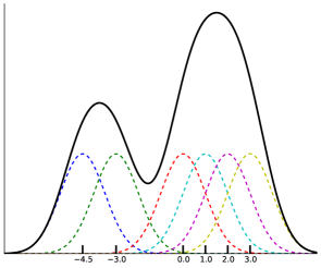
Parzen density estimation is a nonparametric method for estimating the pdf of a distribution empirically from data. For samples $x_{i}$ drawn from a distribution $p$, the parzen window estimate of $p$ can be computed nonparametrically as

$$\hat{p}(x)=\frac{1}{N}\sum_{i=1}^{N}G_{\sigma}(x-x_{i}).$$ (1)

Figure 1: One-dimensional Parzen windowing example with Gaussian kernel functions. A small Gaussian (colored dashed lines) is placed at each sample, the sum of which (solid black line) is used to estimate the pdf from which samples (vertical tick marks) were drawn.

Intuitively, as shown in Fig 1, parzen estimation corresponds to centering a Gaussian kernel at each sample $x_{i}$ drawn from $p$, and then summing to estimate the pdf. The optimal kernel size [14] depends on the density of samples, which approaches zero as the number of samples approaches infinity.

2.2 ITL descriptors

Renyi’s $\alpha$-order entropy for probability density function (pdf) $p$ is given by:

$$H_{\alpha}(X)=\frac{1}{1-\alpha}\log\int p^{\alpha}(x)dx$$ (2)

where $p\in L^{\alpha}$. Renyi’s $\alpha$-order entropy can be considered a generalization of Shannon entropy since $\lim_{\alpha\to 1}H_{\alpha}=\int-\log p(x)dx$, which is Shannon entropy. For the case of $\alpha=2$, equation (2) simplifies to $H_{2}=-\log\int p^{2}(x)dx$ which is known as Renyi’s quadratic entropy.

Plugging (1) into (2), for $\alpha=2$, we obtain:

$$\hat{H}_{2}(X) =-\log\int\left(\frac{1}{N}\sum_{i=1}^{N}G_{\sigma}(x-x_{i})\right)^{2}dx$$ (3)

$$=-\log\left(\frac{1}{N^{2}}\sum_{i=1}^{N}\sum_{j=1}^{N}G_{\sigma\sqrt{2}}(x_{j}-x_{i})\right)$$ (4)

where $G_{\sigma}(x,y)=\frac{1}{\sqrt{2\pi}\sigma}\exp\left(\frac{\|x-y\|^{2}}{2\sigma^{2}}\right)$ is the Gaussian kernel, and $\sigma$ is the kernel size. The argument of the logarithm in equation (4) is called the information potential by analogy with potential fields from physics and is denoted by $\hat{V}_{\sigma}(X)$.

Another important ITL descriptor is Renyi’s cross-entropy which is given by:

$$H_{2}(X,Y)=-\log\int p_{X}(z)p_{Y}(z)dz$$ (5)

Similarly to equation (2), cross-entropy can be estimated by

$$\hat{H}_{2}(X,Y)=-\log\frac{1}{N_{X}N_{Y}}\sum_{i=1}^{N_{X}}\sum_{j=1}^{N_{Y}}G_{\sqrt{2}\sigma}(x_{i}-y_{j})$$ (6)

The argument of the logarithm in equation (5) is called cross-information potential and is denoted $\hat{V}_{\sigma}(X,Y)$. Cross-information potential can be viewed as the average sum of interactions of samples drawn from $p_{X}$ with the estimated pdf $\hat{p}_{Y}$ (or vice-versa).

ITL has also described a number of divergences connected with Renyi’s entropy. In particular, the Euclidean and Cauchy-Schwarz divergences are given by:

$$D {}_{ED}(p_{X}\|p_{Y})=\int\left(p_{X}(z)-p_{Y}(z)\right)^{2}dz$$ (7)

$$=\int p_{X}^{2}(z)dz+\int p_{Y}^{2}(z)dz-2\int p_{X}(z)p_{Y}(z)dz$$ (8)

and

$$D_{CS}(p_{X}\|p_{Y})=-\log\frac{\left(\int p_{X}(z)p_{Y}(z)dz\right)^{2}}{\int p_{X}^{2}(z)dz\int p_{Y}^{2}(z)dz},$$ (9)

respectively. Equations (7) and (9) can be put in terms of information potentials:

$$D_{ED}(p_{X}||p_{Y}) =V(X)+V(Y)-2V(X,Y)$$ (10)

$$D_{CS}(p_{X}||p_{Y}) =\log\frac{V(X)V(Y)}{V^{2}(X,Y)}$$ (11)

Euclidean divergence is so named because it is equivalent to the Euclidean distance between pdfs. Furthermore, it is equivalent to maximum mean discrepancy [15] (MMD) statistical test. Cauchy-Schwarz divergence is named for the Cauchy-Schwarz inequality, which guarantees the divergence is only equal to zero when the pdfs are equal almost everywhere. $D_{CS}$ is symmetric but, unlike $D_{ED}$, does not obey the triangle equality.

Minimizing either divergence over $p_{X}$, i.e., $\min_{p_{X}}D(p_{X}\|p_{Y})$, is a tradeoff between minimizing the information potential (maximizing entropy) of $p_{X}$ and maximizing the cross-information potential (minimizing cross-entropy) of $p_{X}$ with respect to $p_{Y}$. Intuitively, minimizing the information potential encourages samples from $p_{X}$ to spread out, while maximizing the cross-information potential encourages samples from $p_{X}$ to move toward samples from $p_{Y}$.

3 ITL Autoencoders

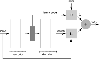
Let us define autoencoders as a 4-tuple $AE=\{E,D,L,R\}$. Where $E$ and $D$ are the encoder and the decoder functions, here parameterized as neural networks. $L$ is the reconstruction cost function that measures the difference between original data samples $x$ and their respective reconstructions $\tilde{x}=D(E(x))$. A typical reconstruction cost is mean-squared error. $R$ is a functional regularization. Here this functional regularization will only be applied to the encoder $E$. Nonetheless, although we are only regularizing the encoder $E$, the interested investigator could also regularize another intermediate layer of the autoencoder .

The general cost function for the ITL-AE can be summarized by the following equation:

$$\text{cost}=L\left(x,\tilde{x}\right)+\lambda R(E,P),$$ (12)

where the strength of regularization is controlled by the scale parameter $\lambda$, and $P$ is the imposed prior.

Figure 2: Block diagram for ITL autoencoder. L is the reconstruction cost function while R is the functional regularization that uses information theoretic measures.

The functional regularization costs investigated in this paper are the ITL Euclidean and Cauchy-Schwarz divergences. Both types of divergence encourage a smooth manifold similar to the imposed prior. That is, maximizing latent code distribution entropy encourages code samples to spread out, while minimizing the cross-entropy between the latent code and the prior distributions encourages code samples to be similar to prior samples.

Note that if the data dimensionality is too high, ITL divergence measures require larger batch sizes to be reliably estimated, this explains why Li et. al. [16] used batches of 1000 samples in their experiments and also why they reduced the data dimensionality with autoencoders. In our own experiments (not shown), the Cauchy-Schwarz divergence worked better than Euclidean for high-dimensional data.

4 Relation to other work

Generative Moment Matching Networks (GMMNs) [16] correspond to the specific case where the input of the decoder $D$ comes from a multidimensional uniform distribution and the reconstruction function $L$ is given by the Euclidean divergence measure. GMMNs could be applied to generate samples from the original input space itself or from a lower dimensional previously trained stacked autoencoder (SCA) [17] hidden space. An advantage of our approach compared to GMMNs is that we can train all the elements in the 4-tuple $AE$ together without the elaborate process of training layerwise stacked autoencoders for dimensionality reduction.

Variational Autoencoders (VAE) [4] adapt a lower bound of the variational regularization, $R$, using parametric, closed form solutions for the KL-divergence. That divergence can be defined using Shannon’s entropy or $H_{\alpha=1}$. Thus, we can also interpret ITL-AE as nonparametric variational autoencoders, where the likelihood of the latent distribution is estimated empirically using Parzen windows. Note that since we can estimate that distribution directly, we do not use the reparametrization trick. Here the reparametrization trick could possibly be used for imposing extra regularization, just like how adding dropout noise regularizes neural networks.

Adversarial autoencoders (AA) [11] have the architecture that inspired our method the most. Instead of using the adversarial trick to impose regularization on the encoder, we defined that regularization from first principles, which allowed us to train a competing method with much fewer trainable parameters. Our most recent experiments show that AA scales better than ITL-AE for high dimensional latent codes. We leave investigation into high dimensional ITL-AE for future work.

Figure 3: Effect of different priors on the function defined by the encoder neural network. a) Swiss-roll, b) Laplacian, b) Gaussian.

5 Experiments

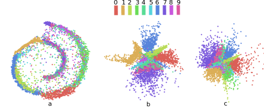
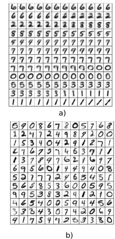
In this section we show experiments using the ITL-AE architecture described in the previous section. First, for a visual interpretation of the effects of variational regularization we trained autoencoders with 2-dimensional latent codes. We used as desired priors a Gaussian, a Laplacian, and a 2D swiss-roll distribution. The resulting codes are shown in Fig. 3. Note that in all of these examples the autoencoder was trained in a completely unsupervised manner. However, given the simplicity of the data and the imposed reconstruction cost, some of the numbers were clustered in separate regions of the latent space. Fig. 4 shows some images obtained by sampling from a linear path on the swiss-roll and random samples from the Gaussian manifold.

For easier comparisons and to avoid extensive hyperparameter search, we constrained our encoder and decoders, $E$ and $D$, to have the same architecture as those used in [11] i.e., each network is a two hidden layer fully connected network with 1000 hidden neurons. Thus, the only hyperparameters investigated in this paper were kernel size $\sigma$ and scale parameter $\lambda$. For the MNIST dataset, the Euclidean distance worked better with smaller kernels, such as $\sigma=1$ or $\sigma=5$, while the Cauchy-Schwarz divergence required larger kernel, $\sigma=10$ for example. Nevertheless, here we will focus in regularizing the low dimensional latent codes and leave experiments using Cauchy-Schwarz divergence for future work.

Our best results for small batch sizes common in deep learning had 3-dimensional latent codes in the output of the encoder, euclidean divergence as the regularization $R$ and mean-squared error as the reconstruction cost $L$. As we will show in the next section, we were able to obtain competitive results and reproduce behaviors obtained by methods trained with larger networks or extra adversarial networks.

Figure 4: Samples from the embedded manifolds. a) samples from a linear walk over the swiss-roll manifold, b) random samples from a zero mean, std 5 Gaussian distribution.

5.1 Log-likelihood analysis

We followed the log-likelihood analysis on the MNIST dataset reported on the literature [18][17][19]. After training ITL-AE on the training set, we generated $10^{4}$ images by inputting $10^{4}$ samples from a $N(0,5)$ distribution to the decoder. Those generated MNIST images were used estimate a distribution using Parzen windows on the high dimensional image space. We calculated the log-likelihood of separate 10k samples from the test set and report the results on Table 1. The kernel size of that Parzen estimator was chose using the best results on a held-out cross-validation dataset. That kernel size was $\sigma=0.16$. Note that our method obtained the second best results between all the compared fully connected generative models. Remember that this was obtained with about $10^{6}$ less adaptive parameters than the best method Adversarial autoencoders.

Table 1: Log-likelihood of MNIST test dataset. Higher the values are better.

Methods	Log-likelihood
Stacked CAE [17]	$121\pm 1.6$
DBN [18]	$138\pm 2$
Deep GSN [19]	$214\pm 1.1$
GAN [10]	$225\pm 2$
GMMN + AE [16]	$282\pm 2$
ITL-AE∗	$300\pm 0.5$
Adversarial Autoencoder [11]	$340\pm 2$
∗ Proposed method.

6 Conclusions

Here we derived and validated the Information Theoretic-Learning Autoencoders, a non-parametric and (optionally) deterministic alternative to Variational Autoencoders. We also revisited ITL for neural networks, but this time, instead of focusing on nonparametric cost functions for non-Gaussian signal processing, we focused on distribution divergences for regularizing deep architectures.

Our results using relatively small, for deep learning standards, 4 layer networks with 3-dimensional latent codes obtained competitive results on the log-likelihood analysis of the MNIST dataset.

Although our results were competitive for fully connected architectures, future work should address the scalability of the ITL estimators for large dimensional latent spaces, which is common on large neural networks and convolutional architectures as well.

References

- [1] Ian Goodfellow, Aaron Courville, and Yoshua Bengio, “Deep learning,” Book in preparation for MIT Press.(Cited on page 159), 2015.
- [2] Yann LeCun, Léon Bottou, Yoshua Bengio, and Patrick Haffner, “Gradient-based learning applied to document recognition,” Proceedings of the IEEE, vol. 86, no. 11, pp. 2278–2324, 1998.
- [3] Nitish Srivastava, Geoffrey Hinton, Alex Krizhevsky, Ilya Sutskever, and Ruslan Salakhutdinov, “Dropout: A simple way to prevent neural networks from overfitting,” The Journal of Machine Learning Research, vol. 15, no. 1, pp. 1929–1958, 2014.
- [4] Diederik P Kingma and Max Welling, “Auto-encoding variational bayes,” arXiv preprint arXiv:1312.6114, 2013.
- [5] Danilo Jimenez Rezende, Shakir Mohamed, and Daan Wierstra, “Stochastic backpropagation and approximate inference in deep generative models,” arXiv preprint arXiv:1401.4082, 2014.
- [6] Jose C Principe, Information theoretic learning: Renyi’s entropy and kernel perspectives, Springer Science & Business Media, 2010.
- [7] W Keith Hastings, “Monte carlo sampling methods using markov chains and their applications,” Biometrika, vol. 57, no. 1, pp. 97–109, 1970.
- [8] Tejas D Kulkarni, Will Whitney, Pushmeet Kohli, and Joshua B Tenenbaum, “Deep convolutional inverse graphics network,” arXiv preprint arXiv:1503.03167, 2015.
- [9] Emily L Denton, Soumith Chintala, Rob Fergus, et al., “Deep generative image models using a? laplacian pyramid of adversarial networks,” in Advances in Neural Information Processing Systems, 2015, pp. 1486–1494.
- [10] Ian Goodfellow, Jean Pouget-Abadie, Mehdi Mirza, Bing Xu, David Warde-Farley, Sherjil Ozair, Aaron Courville, and Yoshua Bengio, “Generative adversarial nets,” in Advances in Neural Information Processing Systems, 2014, pp. 2672–2680.
- [11] Alireza Makhzani, Jonathon Shlens, Navdeep Jaitly, and Ian Goodfellow, “Adversarial autoencoders,” arXiv preprint arXiv:1511.05644, 2015.
- [12] Jose C Principe, Dongxin Xu, and John Fisher, “Information theoretic learning,” Unsupervised adaptive filtering, vol. 1, pp. 265–319, 2000.
- [13] ALFRPED Rrnyi, “On measures of entropy and information,” in Fourth Berkeley symposium on mathematical statistics and probability, 1961, vol. 1, pp. 547–561.
- [14] Bernard W Silverman, Density estimation for statistics and data analysis, vol. 26, CRC press, 1986.
- [15] Arthur Gretton, Karsten M Borgwardt, Malte Rasch, Bernhard Schölkopf, and Alex J Smola, “A kernel method for the two-sample-problem,” in Advances in neural information processing systems, 2006, pp. 513–520.
- [16] Yujia Li, Kevin Swersky, and Richard Zemel, “Generative moment matching networks,” arXiv preprint arXiv:1502.02761, 2015.
- [17] Yoshua Bengio, Grégoire Mesnil, Yann Dauphin, and Salah Rifai, “Better mixing via deep representations,” arXiv preprint arXiv:1207.4404, 2012.
- [18] Geoffrey E Hinton, Simon Osindero, and Yee-Whye Teh, “A fast learning algorithm for deep belief nets,” Neural computation, vol. 18, no. 7, pp. 1527–1554, 2006.
- [19] Yoshua Bengio, Eric Thibodeau-Laufer, Guillaume Alain, and Jason Yosinski, “Deep generative stochastic networks trainable by backprop,” arXiv preprint arXiv:1306.1091, 2013.