A Two-Stage Shape Retrieval (TSR) Method with Global and Local Features
Abstract
A robust two-stage shape retrieval (TSR) method is proposed to address the 2D shape retrieval problem. Most state-of-the-art shape retrieval methods are based on local features matching and ranking. Their retrieval performance is not robust since they may retrieve globally dissimilar shapes in high ranks. To overcome this challenge, we decompose the decision process into two stages. In the first irrelevant cluster filtering (ICF) stage, we consider both global and local features and use them to predict the relevance of gallery shapes with respect to the query. Irrelevant shapes are removed from the candidate shape set. After that, a local-features-based matching and ranking (LMR) method follows in the second stage. We apply the proposed TSR system to MPEG-7, Kimia99 and Tari1000 three datasets and show that it outperforms all other existing methods. The robust retrieval performance of the TSR system is demonstrated.
keywords:
2D shape retrieval , shape representation , MPEG-7 shape dataset , Kimia99 dataset , Tari1000 dataset1 Introduction
2D shapes, also known as silhouette images, are often encountered in computer vision tasks such as manufacture components recognition and retrieval, sketch-based shape retrieval, medical image analysis, etc. Given a 2D shape as the query, a shape retrieval system retrieves ranked shapes from a gallery set according to a certain similarity measure between the query shape and shapes in the retrieval dataset, called gallery shapes. The performance is evaluated by consistency between ranked shapes and human interpretation. The 2D shape retrieval problem is challenging due to a wide range of shape variations, including articulation, noise, contour deformation, topological transformation and multiple projection angles. It is worthwhile to emphasize that our research addresses a retrieval problem with no labeled data at all. It is very different from the deep learning architecture, such as that in [1], that relies on a huge amount of labeled data for training.
Traditionally, the similarity between two shapes is measured using global or local features that capture shape properties such as contours and regions. Global features include the Zernike moment [2] and the Fourier descriptor [3]. They are however not effective in capturing local details of shape contours, resulting in low discriminative performance. Recent research efforts have focused on the development of more powerful local features and post-processing techniques (e.g., diffusion). A substantial progress has been made in this area and will be briefly reviewed below.
The shape context (SC) method [4] describes a contour point by its relationship to other contour points in a local log polar coordination. However, the Euclidian distance used to construct a local coordination is sensitive to articulation variations. The inner-distance shape context (IDSC) method [5] attempts to resolve the articulation problem by using the inner-distance between two points on a contour. The aspect shape context (ASC) method [6] and the articulation invariant representation (AIR) method [7] extend IDSC to account for shape interior variations and projection variations, respectively. Fast computation of the elastic geodesic distance in [8] for shape retrieval is recently studied in [9]. Although local-features-based methods capture important shape properties, their locality restricts discrimination among shapes on the global scale. Consequently, their retrieval results may include globally irrelevant shapes in high ranks. To illustrate this claim, three exemplary query shapes, given in the leftmost column of each row, and their top 10-ranked retrieval results are displayed from left to right in rank order in Figs. 1(a)-(d). The results of the AIR method are shown in the first row of each subfigure. Apparently, these retrieved results are against human intuition.


Post-processing techniques such as the diffusion process (DP) [10], [11], [12], [13], [14] have been proposed to compensate for errors arising from local-features-based shape retrieval methods. The DP treats each sample as a node and the similarity between any two samples corresponds to a weighted edge. All samples form a connected graph, called a manifold, and affinities are diffused along the manifold to improve measured similarities. However, the DP has its limitations. When shapes of two classes are mixed in the feature space, it cannot separate them properly. Also, when a query is far away from the majority of samples in its class, it is difficult to retrieve shapes of the same class with high ranks. For example, AIR is confused with several classes as shown in the first row of Figs. 1(a)-(d). Even the best DP does not help retrieval results much as shown in the second row of Figs. 1 (a)-(d). Clearly, the DP is constrained by the underlying feature space.
Being motivated by the above observations, we develop a more robust shape retrieval system with two main contributions in this paper. First, we consider both global and local features. Since traditional global features are not discriminative enough, we develop more powerful and robust global features. Second, we propose a two-stage shape retrieval (TSR) system that consists of: I) the irrelevant cluster filtering (ICF) stage and II) the local-features-based matching and ranking (LMR) stage. For Stage II, we can adopt any state-of-the-art shape retrieval solution, and our focus is on the design of Stage I. The robustness of the proposed TSR system can be intuitively explained below. In the ICF stage (Stage I), we attempt to cluster gallery shapes that are similar to each other by examining global and local features simultaneously. Two contradictory cases may arise. Shapes that are close in the local feature space can be distant in the global feature space, and vice versa. Here, we resolve the contradiction with a joint cost function that strikes a balance between the two distances. It is convenient to use the ICF stage to filter out unlikely shapes. In particular, shapes that are close in the local feature space but distant in the global feature can be removed in this stage. Then, the TSR system will avoid the same mistake of traditional one-stage matching methods when it proceeds to its second LMR stage. The retrieved results of the TSR system are shown in the third row of Figs. 1 (a)-(d). All wrongly retrieved results are corrected by TSR. The novelty of our work lies in two areas: 1) identifying the cause of unreliable retrieval results in all state-of-the-art methods for the 2D shape retrieval problem, and 2) finding a new system-level framework to solve this problem.
2 Proposed TSR Method
2.1 System Overview
An overview flow chart of the proposed TSR system is given in Fig. 2. As shown in the figure, the system consists of two stages. Stage I of the TSR system is trained in an off-line process with the following three steps.
-
1.
Initial clustering. All samples in the dataset are clustered using their local features.
-
2.
Classifier Training. Samples close to the centroid of each cluster are selected as training data. Their extracted global features are used to train a random forest classifier.
-
3.
Relevant Clusters Assignment. The trained random forest classifier assigns relevant clusters to all samples in the dataset so that each sample is associated with a small set of relevant clusters.
In the on-line query process, we extract both global and local features from a query shape and, then, proceed with the following two steps:
-
1.
Predicting Relevant Clusters. Given a query sample, we assign it a set of relevant clusters based on a cost function. The cost function consists of two negative log likelihood terms. One likelihood reflects the relevant cluster distribution of the query sample itself while the other is the mean of the relevant cluster distributions of its local neighbors. The ultimate relevant clusters are obtained by thresholding the cost function.
-
2.
Local Matching and Ranking. We conduct matching and ranking for samples in the relevant clusters with a distance in the local feature space. The diffusion process can also be applied to enhance the retrieval accuracy.

A query bell shape is given in Fig. 2. The traditional shape retrieval algorithm (with Stage II only) finds birds, a bell and a beetle in the top six ranks. However, the clusters of birds and beetles are not relevant to the bell shape as predicted by the trained classifier. Since they are removed from the candidate set in Stage II, the mistake can be avoided. After the processing of Stage I, the retrieved top 6 samples are all bell shapes. We will describe the processing in Stages I and II in detail below.
2.2 The ICF Stage (Stage I)
Shape Normalization. Each shape is normalized so that it is invariant against translation, scaling and rotation. Translational invariance is achieved by aligning the shape centroid and the image center. For rotational invariance, we align the dominant reflection symmetry axis, which passes through the shape centroid and has the maximum symmetry value, vertically. After rotational normalization, we set the larger side (width or height) of the shape to unity for scale invariance. Examples of shape normalization are given in Fig. 3, where the first and third rows are the original shapes while the second and forth rows are their corresponding normalized results. Although normalization based on the dominant reflection symmetry axis works well in general in our experiments, it is worthwhile to point out that, if samples of a class do not contain a clear dominant reflection axis, their normalized poses may not be well aligned (e.g., the three running men in the third row of Fig. 3). However, there still exist rotational invariant global features in TSR to compensate for the articulational variation. After shape normalization, we perform hole-filling and contour smoothing to remove the interior holes and contour noise, respectively.
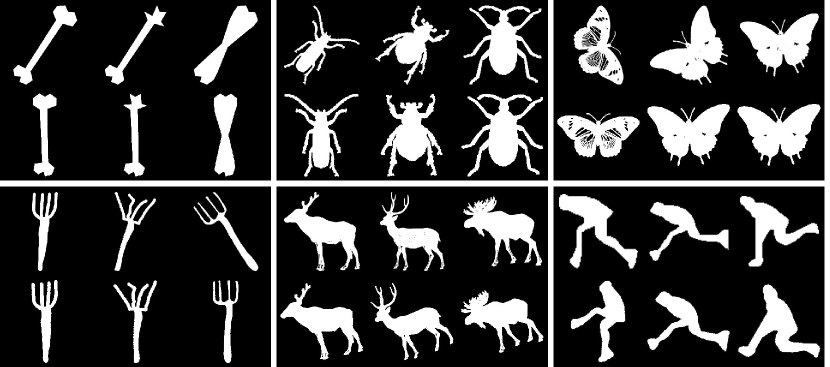
Global Features. To capture the global layout of a shape, we consider three feature types: 1) skeleton features, 2) wavelet features, and 3) geometrical features.
For skeleton features, we extract the basic structural information of a shape while ignoring minor details due to contour variations. We first apply the thinning algorithm [15] to obtain the initial skeleton. Then, a pruning process is developed to extract its clean skeleton without over-simplification. We show several input shapes and their initial and pruned skeletons in Fig. 4. After getting a clean skeleton, we consider four types of salient points: 1) turning points (that have a sharp curvature change), 2) end points, 3) T-junction points and 4) cross-junction points. The numbers of these four salient points form a 4D skeleton feature vector denoted by . Skeleton features of the six shapes in Fig. 4 are given in Table 1. They are rotational, translational and scaling invariant.
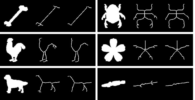
| Nos. of Salient pts | bone | beetle | chicken | device0 | dog | fish |
|---|---|---|---|---|---|---|
| turning pts | 2 | 4 | 3 | 0 | 1 | 0 |
| end pts | 2 | 6 | 4 | 5 | 5 | 2 |
| T-junction pts | 0 | 2 | 2 | 0 | 3 | 0 |
| cross-junction pts | 0 | 1 | 0 | 1 | 0 | 0 |
For wavelet features, Haar-like filters were adopted for face detection in [16]. Being motivated by this idea, we adopt five Haar-like filters as shown in Fig. 5 to extract wavelet features. For a normalized shape, the first two filters are used to capture the 2-band symmetry while the middle two filters are used to capture the 3-band symmetry horizontally and vertically. The last one is used to capture the cross diagonal symmetry. The responses of the five filters form a 5D wavelet feature vector denoted by .

Furthermore, we incorporate the following four geometrical features [15]: 1) aspect ratio, 2) circularity, 3) symmetry and 4) solidity. The aspect ratio is the ratio of the width and height of the bounding box of a shape. The circularity is set to , where is the area and is the perimeter of the shape. The aspect ratio and circularity are closer to one, if a shape is closer to a square or a circle. If a shape is closer a long bar, its aspect ratio and circularity are closer to zero. The symmetry is computed based on the dominant reflection symmetry axis of a shape. The solidity of a shape is the ratio of its area and the area of its convex hull. If a shape is a convex set, its solidity is unity. Otherwise, it will be less than one. These four geometric features form a 4D geometrical feature vector denoted by .
Shape Clustering. In the traditional 2D shape retrieval formulation, all shapes in the dataset are not labeled. Under this extreme case, we use the spectral clustering algorithm [17] to reveal the underlying relationship between gallery shapes based on local features. For the MPEG-7 dataset, shapes in several clusters using the AIR feature are shown in Fig. 6. Some clusters look reasonable while others do not. Actually, any unsupervised clustering method will encounter the following two challenges. First, uncertainty occurs near cluster boundaries so that samples near boundaries have a higher probability of being wrongly clustered. Second, the total number of shape classes is unknown. When the cluster number is larger than the class number in the database, the clustering algorithm creates sub-classes or even mixed classes. The relationship between them has to be investigated.
To address the first challenge, we extract samples closest to the centroid of the th cluster and assign them a cluster label. Clearly, samples sharing the same cluster label are close to each other in the feature space. There is a trade-off in choosing a proper value of . A smaller value guarantees higher clustering accuracy but fewer gallery samples will be assigned cluster labels. Empirically, we set the value of to one half of the size of the th cluster. To address the second challenge, we use local features to conduct clustering and assign cluster labels to a subset of samples. These labeled samples are used to train a random forest classifier [18] with their global features. Finally, all gallery shapes are treated as testing samples. The random forest classifier is used to predict the probability of each cluster type for them by voting. In this way, samples that are clustered in the local feature space can be linked to multiple clusters probabilistically due to similarities in the global feature space.
Typically, a random forest classifier reduces the influence of outliers by bootstrapping. When the training data size is small, it is difficult to predict outliers in testing samples accurately. It is possible for the classifier to terminate a decision process in an early stage due to a shared dominating feature between the testing sample and the training samples. One example is shown in Fig. 7, where the “sword-like” fish sample in the red box is clearly an outlier with respect to other fish samples. If all fish samples except for the outlying sample are used as training samples, the aspect ratio is an important feature for the fish class since its value is consistent among all training fish samples. When we use the sword-like fish as a testing sample, this feature will dominate and terminate the decision process early with a wrong predicted result. Namely, it would be a sword rather than a fish. To overcome this problem, we train multiple random forest classifiers using different feature subsets to suppress the impact from a dominating feature. Finally, we combine the results of these classifiers by the sum rule to obtain the final prediction.

Cluster Relevance Assignment. The output of the ICF stage includes: 1) a set of indexed clusters and 2) soft classification (or multi-labeling) of all gallery samples. For item #1, we use the unsupervised spectral clustering algorithm to generate clusters as described above. If the class number is known (or can be estimated), it is desired that the cluster number is larger than the class number. Each of these clusters is indexed by a cluster ID. For item #2, we adopt soft classification so that each sample can be associated with multiple clusters. This is done for two reasons. If two sub-classes belong to the same ground truth class, we need a mechanism to regroup them together. Clearly, a hard classification process does not allow this to happen. Second, a hard classification error cannot be easily compensated while a soft classification error is not as fatal and it is likely to be fixed in the LMR stage (stage II) of the TSR system.
We consider two relevant clusters assignment schemes below.
1) Direct Assignment
We apply the random forest classifier to both training and testing
samples based on their global features. Then, the probability for the
th shape sample (denoted by ) belongs to the th cluster
denoted by can be estimated by the following normalized voting
result:
| (1) |
where is the number of votes claiming that belongs to . Eq. (1) associates to its relevant clusters directly.
2) Indirect Assignment
Intuitively, a good cluster relevance assignment scheme should take both
global and local features into account. This can be achieved as follows.
For query sample , we find its nearest neighbors (denoted by
) using a certain distance function in a local feature space (e.g.
the same feature space used in IDSC or AIR). Then, the probability of
belonging to can be estimated by the weighted sum of the
probability in Eq. (1) in form of
| (2) |
Eq. (2) associates to its relevant clusters indirectly. That is, the assignment is obtained by averaging the relevant clusters assignment of its nearest neighbors. Empirically, we choose K to be 1.5 times the average cluster size in the experiments.
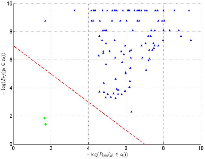
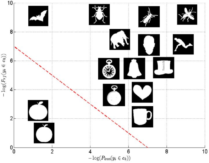
We show an example that assigns a query apple shape to its relevant clusters in Fig. 8(a), whose x-axis and y-axis are the negative log functions of Eqs. (1) and (2), respectively. Every dot in Fig. 8(a) represents a cluster after the shape clustering process. To visualize shapes represented by a dot, we plot a representative sample of each cluster in Fig. 8(b).
We see that the distance between the bat cluster and the apple cluster is short in the x-axis but long in the y-axis. This is because that samples of the apple and bat clusters are interleaved in the local feature space. This is evidenced in the retrieval results of AIR in Fig. 1(a). However, the apple and bat clusters have little intersection in the global feature space. On the other hand, the cup and apple clusters have large intersection in the global feature space. Yet, their distance is far in the local feature space. It is apparent that Eqs. (1) and (2) provide complementary relevance assignment strategies for query sample . It is best to integrate the two into one assignment scheme. For example, we can draw a line to separate relevant and irrelevant clusters with respect to the query apple shape in this plot.
Mathematically, we define a cost function as follows
| (3) |
We compute for all clusters . If
| (4) |
where is a pre-selected threshold, we say that cluster is a relevant cluster for query . Otherwise, it is irrelevant.
2.3 The LMR Stage (Stage II)
In the LMS stage, we rank the similarity of shapes in the retrieved relevant clusters by using a local-features-based matching scheme (e.g., AIR) including a diffusion process. We adopt the Local Constrained Diffusion Process (LCDP) from [10] in the TSR system. The diffusion process is slightly modified with the availability of relevant clusters in the TSR system since the diffusion process can be conducted on a more reasonable manifold due to the processing in Stage I.
3 Experimental Results
We demonstrate the retrieval performance of the proposed TSR system by conducting experiments on three shape datasets: MPEG-7, Kimia99 and Tari1000. We set the threshold of the cost function in Eq. (4) to 7 empirically for all experiments. We also consider the incorporation of two diffusion processes in various schemes. They are denoted by:
MPEG-7 Shape Dataset. The MPEG-7 shape dataset [19], which remains to be the largest and most challenging, contains 1400 shape samples in 70 independent classes. Samples are uniformly distributed so that each class has shape samples. The retrieval performance is measured by the bull’s eye score, which means the percentage of shapes sharing the same class with a query in the top retrieved shapes. AIR and DP1 are used as the local feature space and the diffusion process in the TSR method, respectively.
| Cluster Numbers (M) | 16 | 32 | 48 | 64 | 80 | 96 | 112 | 128 |
|---|---|---|---|---|---|---|---|---|
| TSR (ICF+AIR) | 96.00% | 97.54% | 98.81% | 99.51% | 99.62% | 99.85% | 99.92% | 99.90% |
| TSR (ICF+AIR+DP1) | 98.32% | 98.90% | 99.72% | 99.99% | 99.99% | 99.99% | 100.00% | 99.99% |
We first show the bull’s eye scores of two TSR schemes using a different cluster number in the shape clustering step in Table 2. Both TSR methods adopt the AIR features for the distance computation. However, one of them uses DP1 while the other does not. Since TSR(ICF+AIR+DP1) offers better performance, we choose it as the default TSR configuration for the MPEG-7 shape dataset. Generally speaking, the performance degrades when is small due to the loss of discriminability in larger cluster sizes. The retrieval performance improves as the cluster number increases up to 112. After that, the performance saturates and could even drop slightly. That means that we lose the advantage of clustering when the cluster size is too small. For the remaining MPEG-7 dataset experimental results, we choose .
The bull’s eye scores of the TSR method and several state-of-the-art methods are compared in Table 3. Both TSR and AIR+DP2 reach 100%. The bull’s eye score is one of the popular retrieval performance measures for the 2D shape retrieval problem.
| Method | Bull’s eye score |
|---|---|
| CSS [20] | 75.44% |
| IDSC [5] | 85.40% |
| ASC [6] | 88.30% |
| HF [21] | 89.66% |
| AIR [7] | 93.67% |
| IDSC+DP1 [13] | 93.32% |
| ASC+DP1 [6] | 95.96% |
| IDSC+SC+Co-Transduction [22] | 97.72% |
| AIR+TPG [14] | 99.90% |
| AIR+DP2 [10] | 100.00% |
| Proposed TSR (ICF+AIR+DP1) | 100.00% |
| N | 20 | 25 | 30 | 35 | 40 |
|---|---|---|---|---|---|
| IDSC | 77.21% | 80.44% | 82.61% | 84.16% | 85.40% |
| IDSC+DP1 | 88.53% | 90.78% | 92.03% | 92.73% | 93.32% |
| AIR | 88.17% | 89.99% | 91.28% | 92.64% | 93.67% |
| AIR+DP2 | 94.42% | 97.92% | 98.66% | 99.38% | 100% |
| Proposed TSR | 98.46% | 99.09% | 99.40% | 99.71% | 100% |
However, since each MPEG-7 shape class contains 20 shape samples, the measure of correctly retrieved samples from the top 40 ranks cannot reflect the true power of the proposed TSR method. To push the retrieval performance further, we compare the accuracy of retrieved results from the top 20, 25, 30, 35 and 40 ranks of TSR and several state-of-the-art methods in Table 4 whose last column corresponds the bull’s eye scores reported in Table 3. The superiority of TSR stands out clearly in this table.
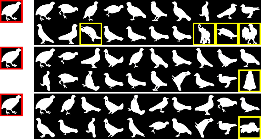
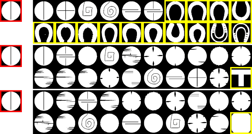
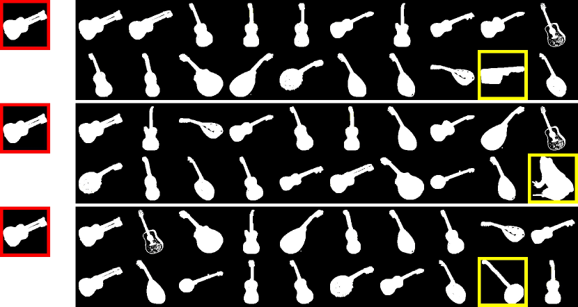
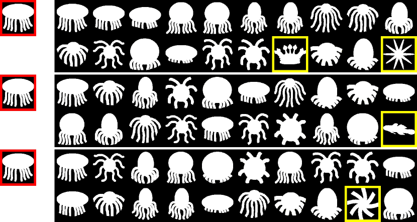
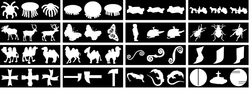
When , TSR can retrieve 20 shapes of the entire class correctly with respect to most query samples. However, it still makes mistakes occasionally. It is worthwhile to show these erroneous cases to have further insights. For this reason, we conduct error analysis in Figs. 9(a)-(d). The performance of IDSC+DP1 is clearly worse than that of AIR+DP2 and TSR. AIR+DP2 makes mistakes between bird/bell, circle/device8, guitar/frog and octopus/fish as shown in the second black stripes of all subfigures. This type of mistakes is not consistent with human visual experience. In contrast, TSR makes mistakes between bird/truck , device9/device3, guitar/spoon, octopus/device2 as shown in the third black stripes of all subfigures. These mistakes are closer to human visual experience. Actually, these wrongly retrieved shapes are similar to the query shape in their global attributes as a result of the special design of the TSR system.
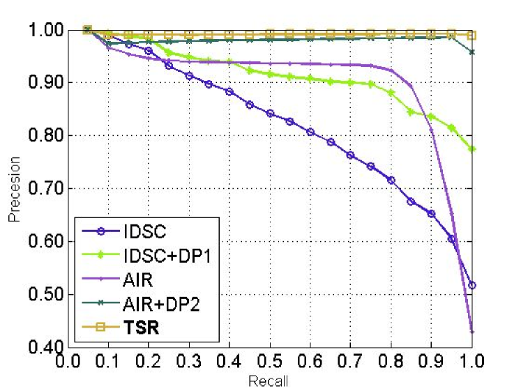
For further performance benchmarking, we show the precision-and-recall curves of TSR and several methods in Fig. 10. We see from the figure that TSR outperforms all other methods by a significant margin except for AIR+DP2.
Kimia99 Shape Dataset. The MPEG-7 shape dataset contains primarily articulation and contour deformation variations. We also conduct experiments on the Kimia99 shape dataset [23] that contains other variations such as occlusions and distorted parts. However, this dataset is relatively small. It contains 99 shapes in total, which are classified into 9 classes. Each class has 11 shapes. For this dataset, we choose IDSC as the local feature extraction and ranking method and DP1 as the diffusion process in the LMR stage as the default TSR method. The number of clusters is set to 15.
| Method | 1st | 2nd | 3rd | 4th | 5th | 6th | 7th | 8th | 9th | 10th |
|---|---|---|---|---|---|---|---|---|---|---|
| SC[4] | 97 | 91 | 88 | 85 | 84 | 77 | 75 | 66 | 56 | 37 |
| Gen. Model [24] | 99 | 97 | 99 | 98 | 96 | 96 | 94 | 83 | 75 | 48 |
| Path Similarity [25] | 99 | 99 | 99 | 99 | 96 | 97 | 95 | 93 | 89 | 73 |
| Shock Edit [23] | 99 | 99 | 99 | 98 | 98 | 97 | 96 | 95 | 93 | 82 |
| Triangle Area [26] | 99 | 99 | 99 | 98 | 98 | 97 | 97 | 98 | 94 | 79 |
| Shape Tree [27] | 99 | 99 | 99 | 99 | 99 | 99 | 99 | 97 | 93 | 86 |
| IDSC[5] | 99 | 99 | 99 | 98 | 98 | 97 | 97 | 98 | 94 | 79 |
| IDSC+GT[28] | 99 | 99 | 99 | 99 | 99 | 99 | 99 | 99 | 97 | 99 |
| Proposed TSR | 99 | 99 | 99 | 99 | 99 | 99 | 99 | 99 | 99 | 99 |
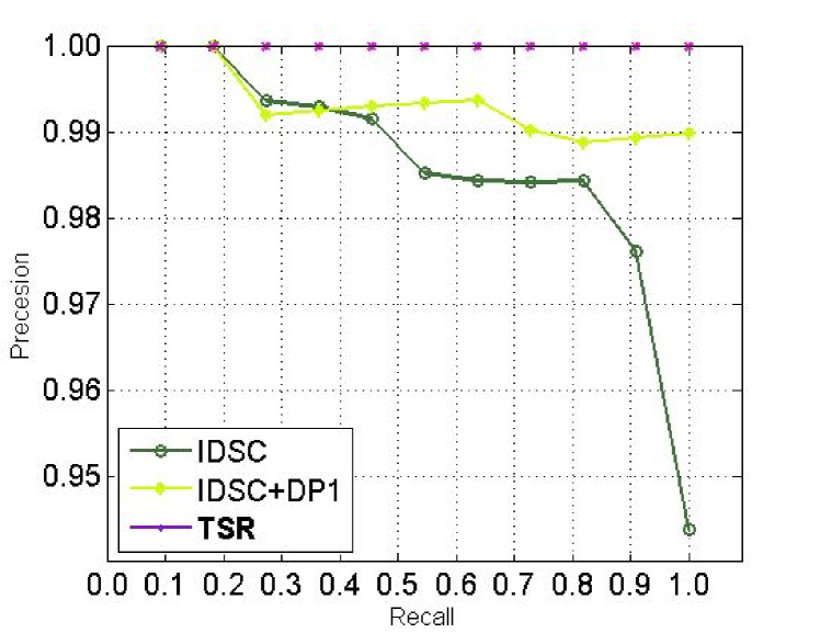
The common evaluation criterion for this dataset is top (with ) consistency, which measures consistency at the top retrieved shapes against each query. Note that the best possible value is 99, which is summed up by consistency of all 99 query samples. The top consistency results of several methods are compared in Table 5. The TSR method can exclude round 75% irrelevant shapes for each query and effectively improve the IDSC result. The TSR method can achieve the highest consistency, namely, 99, for all possible values. The precision-and-recall curves of IDSC, IDSC+DP1 and TSR are shown in Fig. 11. We conclude that the TSR method does not make any mistake in shape retrieval against the Kimia99 Shape Dataset as supported by data in Table 5 and Fig. 11.
| Method | Bull’s eye score |
|---|---|
| SC [4] | 94.17% |
| IDSC [5] | 95.33% |
| ASC [6] | 95.44% |
| IDSC+GT [28] | 99.35% |
| IDSC+LCDP [22] | 99.70% |
| IDSC+DDGM+Co-Transduction [22] | 99.995% |
| Proposed TSR | 100.00% |
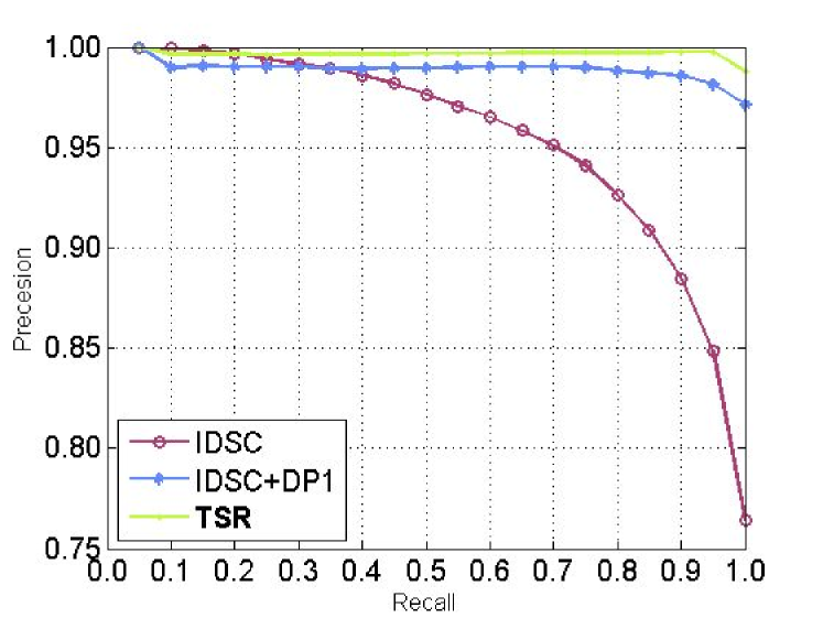
Tari1000 Shape Dataset. We test the TSR method on a new dataset called Tari1000 [29]. Tari1000 consists 1000 shapes classified into 50 classes. Each class has 20 shapes. As compared to the MPEG-7 dataset, Tari1000 contains more deformation and articulation variations. Here, we adopt IDSC as the local feature extraction and ranking method and DP1 as the diffusion process in the LMR stage as the default TSR method. The number of clusters is set to 75. The bull’s eye scores of several methods are compared in Table 6 and the Precision and Recall curves are shown in Fig. 12. We see that TSR can achieve the perfect Bull’s eye score (100%) which proves its robustness against severe articulations.
4 Conclusion
A robust two-stage shape retrieval (TSR) method was proposed to solve the 2D shape retrieval problem. In the ICF stage, the TSR method explores the underlying global properties of 2D shapes. Irrelevant shape clusters are removed for each query shape. In the LMR stage, the TSR method only need to focus on the matching and ranking in a much smaller subset of shapes. We conducted thorough retrieval performance evaluation on three popular datasets - MPEG7, Kimia99 and Tari1000. The TSR method retrieves more globally similar shapes and achieves the highest retrieval accuracy as compared with its benchmarking methods.
Acknowledgment
Computation for the work described in this paper was supported by the University of Southern California’s Center for High-Performance Computing (hpc.usc.edu).
References
- [1] A. Krizhevsky, I. Sutskever, G. E. Hinton, Imagenet classification with deep convolutional neural networks, in: Advances in neural information processing systems, 2012, pp. 1097–1105.
- [2] A. Khotanzad, Y. H. Hong, Invariant image recognition by zernike moments, Pattern Analysis and Machine Intelligence, IEEE Transactions on 12 (5) (1990) 489–497.
- [3] D. Zhang, G. Lu, Shape-based image retrieval using generic fourier descriptor, Signal Processing: Image Communication 17 (10) (2002) 825–848.
- [4] S. Belongie, J. Malik, J. Puzicha, Shape matching and object recognition using shape contexts, Pattern Analysis and Machine Intelligence, IEEE Transactions on 24 (4) (2002) 509–522.
- [5] H. Ling, D. W. Jacobs, Shape classification using the inner-distance, Pattern Analysis and Machine Intelligence, IEEE Transactions on 29 (2) (2007) 286–299.
- [6] H. Ling, X. Yang, L. J. Latecki, Balancing deformability and discriminability for shape matching, in: Computer Vision–ECCV 2010, Springer, 2010, pp. 411–424.
- [7] R. Gopalan, P. Turaga, R. Chellappa, Articulation-invariant representation of non-planar shapes, in: Computer Vision–ECCV 2010, Springer, 2010, pp. 286–299.
- [8] A. Srivastava, E. Klassen, S. H. Joshi, I. H. Jermyn, Shape analysis of elastic curves in euclidean spaces, Pattern Analysis and Machine Intelligence, IEEE Transactions on 33 (7) (2011) 1415–1428.
- [9] G. Dogan, J. Bernal, C. R. Hagwood, A fast algorithm for elastic shape distances between closed planar curves, in: Proceedings of the IEEE Conference on Computer Vision and Pattern Recognition, 2015, pp. 4222–4230.
- [10] M. Donoser, H. Bischof, Diffusion processes for retrieval revisited, in: Computer Vision and Pattern Recognition (CVPR), 2013 IEEE Conference on, IEEE, 2013, pp. 1320–1327.
- [11] V. Premachandran, R. Kakarala, Consensus of k-nns for robust neighborhood selection on graph-based manifolds, in: Computer Vision and Pattern Recognition (CVPR), 2013 IEEE Conference on, IEEE, 2013, pp. 1594–1601.
- [12] N. Qadeer, D. Hu, X. Liu, S. Anwar, M. S. Sultan, Improving shape retrieval by integrating air and modified mutual nn graph, Advances in Multimedia 2015.
- [13] X. Yang, S. Koknar-Tezel, L. J. Latecki, Locally constrained diffusion process on locally densified distance spaces with applications to shape retrieval, in: Computer Vision and Pattern Recognition, 2009. CVPR 2009. IEEE Conference on, IEEE, 2009, pp. 357–364.
- [14] X. Yang, L. Prasad, L. J. Latecki, Affinity learning with diffusion on tensor product graph, Pattern Analysis and Machine Intelligence, IEEE Transactions on 35 (1) (2013) 28–38.
- [15] W. K. Pratt, Digital Image Processing: PIKS Scientific Inside, Wiley-Interscience, 2007.
- [16] P. Viola, M. J. Jones, D. Snow, Detecting pedestrians using patterns of motion and appearance, International Journal of Computer Vision 63 (2) (2005) 153–161.
- [17] A. Y. Ng, M. I. Jordan, Y. Weiss, et al., On spectral clustering: Analysis and an algorithm, Advances in neural information processing systems 2 (2002) 849–856.
- [18] L. Breiman, Random forests, Machine learning 45 (1) (2001) 5–32.
- [19] L. J. Latecki, R. Lakämper, U. Eckhardt, Shape descriptors for non-rigid shapes with a single closed contour, in: Computer Vision and Pattern Recognition, 2000. Proceedings. IEEE Conference on, Vol. 1, IEEE, 2000, pp. 424–429.
- [20] F. Mokhtarian, S. Abbasi, J. Kittler, et al., Efficient and robust retrieval by shape content through curvature scale space, Series on Software Engineering and Knowledge Engineering 8 (1997) 51–58.
- [21] J. Wang, X. Bai, X. You, W. Liu, L. J. Latecki, Shape matching and classification using height functions, Pattern Recognition Letters 33 (2) (2012) 134–143.
- [22] X. Bai, B. Wang, C. Yao, W. Liu, Z. Tu, Co-transduction for shape retrieval, Image Processing, IEEE Transactions on 21 (5) (2012) 2747–2757.
- [23] T. B. Sebastian, P. N. Klein, B. B. Kimia, Recognition of shapes by editing their shock graphs, Pattern Analysis and Machine Intelligence, IEEE Transactions on 26 (5) (2004) 550–571.
- [24] Z. Tu, A. L. Yuille, Shape matching and recognition–using generative models and informative features, in: Computer Vision-ECCV 2004, Springer, 2004, pp. 195–209.
- [25] X. Bai, L. J. Latecki, Path similarity skeleton graph matching, Pattern Analysis and Machine Intelligence, IEEE Transactions on 30 (7) (2008) 1282–1292.
- [26] N. Alajlan, M. S. Kamel, G. H. Freeman, Geometry-based image retrieval in binary image databases, Pattern Analysis and Machine Intelligence, IEEE Transactions on 30 (6) (2008) 1003–1013.
- [27] P. F. Felzenszwalb, J. D. Schwartz, Hierarchical matching of deformable shapes, in: Computer Vision and Pattern Recognition, 2007. CVPR’07. IEEE Conference on, IEEE, 2007, pp. 1–8.
- [28] X. Bai, X. Yang, L. J. Latecki, W. Liu, Z. Tu, Learning context-sensitive shape similarity by graph transduction, Pattern Analysis and Machine Intelligence, IEEE Transactions on 32 (5) (2010) 861–874.
- [29] C. Aslan, A. Erdem, E. Erdem, S. Tari, Disconnected skeleton: Shape at its absolute scale, Pattern Analysis and Machine Intelligence, IEEE Transactions on 30 (12) (2008) 2188–2203.