Subdiffusion in a system consisting of two different media separated by a thin membrane

Tadeusz Kosztołowicz
(Institute of Physics, Jan Kochanowski University,
ul. Świȩtokrzyska 15, 25-406 Kielce, Poland
e-mail: tadeusz.kosztolowicz@ujk.edu.pl
)
Abstract

We consider subdiffusion in a system which consists of two media separated by a thin membrane. The subdiffusion parameters may be different in each of the medium. Using the new method presented in this paper we derive the probabilities (the Green’s functions) describing a particle’s random walk in the system. Within this method we firstly consider the particle’s random walk in a system with both discrete time and space variables in which a particle can vanish due to reactions with constant probabilities R1subscript𝑅1R_{1} and R2subscript𝑅2R_{2} defined separately for each medium. Then, we move from discrete to continuous variables. The reactions included in the model play a supporting role. We link the reaction probabilities with the other subdiffusion parameters which characterize the media by means of the formulae presented in this paper. Calculating the generating functions for the difference equations describing the random walk in the composite membrane system with reactions, which depend explicitly on R1subscript𝑅1R_{1} and R2subscript𝑅2R_{2}, we are able to correctly incorporate the subdiffusion parameters of both the media into the Green’s functions. Finally, placing R1=R2=0subscript𝑅1subscript𝑅20R_{1}=R_{2}=0 into the obtained functions we get the Green’s functions for the composite membrane system without any reactions. From the obtained Green’s functions, we derive the boundary conditions at the thin membrane. One of the boundary conditions contains the Riemann–Liouville fractional time derivatives, which show that the additional ‘memory effect’ is created by a discontinuoity of the system. The second boundary condition demands continuity of a flux at the membrane.

keywords: subdiffusion, diffusion in composite systems with a thin membrane, random walk model

1 Introduction

In the many processes considered in biological, engineering or physical sciences normal diffusion or subdiffusion occurs in a system composed of two media, separated by a partially permeable thin membrane; in each part of the system different parameters characterizing diffusion may occur. As an example, we mention the transport of various substances (glucose, pyruvate, lactate, alanine) between blood and a cell [1], diffusion of various substances (medications, cosmetics) through the skin [2], diffusion of various substances in the brain [3], diffusion between extracellular brain space and cells [4], diffusion of large molecular drugs into the brain [5], nisin diffusion into agarose gel [6, 7]. A list of similar examples can be significantly expanded, see also the problems discussed in [8, 9, 10].

Subdiffusion is usually defined as a random walk process in which [11]

(Δx)2=2DtαΓ(1+α),delimited-⟨⟩superscriptΔ𝑥22𝐷superscript𝑡𝛼Γ1𝛼\left\langle(\Delta x)^{2}\right\rangle=\frac{2Dt^{\alpha}}{\Gamma(1+\alpha)}\;, (1)

where (Δx)2delimited-⟨⟩superscriptΔ𝑥2\left\langle(\Delta x)^{2}\right\rangle is the mean square displacement of a random walker, α𝛼\alpha is a subdiffusion parameter (0<α<10𝛼10<\alpha<1), D𝐷D is a subdiffusion coefficient, measured in units m2/sαsuperscript𝑚2superscript𝑠𝛼m^{2}/s^{\alpha}, and ΓΓ\Gamma denotes the Gamma function. The process of subdiffusion can occur in media in which particles’ movement is greatly hindered due to the internal structure of a medium such as, for example, in gels [12, 13, 14]. Subdiffusion is usually described by the following subdiffusion equation with the Riemann–Liouville fractional time derivative (here 0<α<10𝛼10<\alpha<1) [11]

C(x,t)t=D1αt1α2C(x,t)x2.𝐶𝑥𝑡𝑡𝐷superscript1𝛼superscript𝑡1𝛼superscript2𝐶𝑥𝑡superscript𝑥2\frac{\partial C(x,t)}{\partial t}=D\frac{\partial^{1-\alpha}}{\partial t^{1-\alpha}}\frac{\partial^{2}C(x,t)}{\partial x^{2}}\;. (2)

The Riemann–Liouville fractional derivative is defined as being valid for δ>0𝛿0\delta>0 (here k𝑘k is a natural number which fulfils k1δ<k𝑘1𝛿𝑘k-1\leq\delta<k)

dδf(t)dtδ=1Γ(kδ)dkdtk0t(tt)kδ1f(t)𝑑t.superscript𝑑𝛿𝑓𝑡𝑑superscript𝑡𝛿1Γ𝑘𝛿superscript𝑑𝑘𝑑superscript𝑡𝑘superscriptsubscript0𝑡superscript𝑡superscript𝑡𝑘𝛿1𝑓superscript𝑡differential-dsuperscript𝑡\frac{d^{\delta}f(t)}{dt^{\delta}}=\frac{1}{\Gamma(k-\delta)}\frac{d^{k}}{dt^{k}}\int_{0}^{t}{(t-t^{\prime})^{k-\delta-1}f(t^{\prime})dt^{\prime}}\;. (3)

For α=1𝛼1\alpha=1 one obtains a normal diffusion equation.

We consider subdiffusion in a system which consists of two media separated by a thin partially permeable membrane. In each part of the system, bounded by the membrane, there may be different subdiffusion parameters. We assume that the system is homogeneous in a plane perpendicular to the x𝑥x axis, thus the system is effectively one–dimensional. The thin membrane is treated here as a partially permeable wall. A diffusing particle which tries to pass through the membrane can be stopped by the membrane with some probability or can jump through the membrane to another part of the system. The membrane is assumed to be so thin that the particle’s random walk inside the membrane is not considered. To solve the subdiffusion equation in a membrane system, two boundary conditions at the membrane are needed. However, until now, various boundary conditions which are not equivalent to one another have been assumed at the membrane, see for example [15, 16, 17, 18, 19, 20, 21, 22, 23, 24, 25, 26, 27, 28, 29, 30, 31, 32, 33, 34, 35, 36, 37].

We present the method of deriving the probability P(x,t;x0)𝑃𝑥𝑡subscript𝑥0P(x,t;x_{0}) (the Green’s function) of finding a particle at point x𝑥x at time t𝑡t, x0subscript𝑥0x_{0} is the initial position of a particle in the composite system with a thin membrane. We derive the Green’s functions using a simple random walk model with both discrete time and spatial variables. Next we move to the continuous variables by means of the procedure presented in this paper. From the Green’s functions we derive boundary conditions at a thin membrane. In the paper [24] the method based on the random walk model on a lattice was used to determine the Green’s functions for a system with a thin membrane in which the homogeneous medium is divided by a thin membrane into two parts. However, this method is not applicable to the system in which the subdiffusion parameters are different at each part of the system. In this paper we present a new method of deriving the Green’s functions for the composite system with a thin membrane.

A random walk model with a discrete time and space variable appears to be a useful tool in modeling anomalous or normal diffusion [38, 39, 40, 41, 42, 43]. This model is particularly conducive in determining the Green’s function for a system in which the uniformity of a system is disturbed at one point [43, 44, 45, 46, 47]; in this paper the point represents a membrane which is located perpendicularly to the x𝑥x axis in a one–dimensional system. In order to move from discrete to continuous time in a homogeneous system one assumes that the time which is needed for a particle to take its next step is ruled by the distribution ω(t)𝜔𝑡\omega(t). However, the situation is more complicated in a system which consists of two parts with different transport properties since the two distributions ω1(t)subscript𝜔1𝑡\omega_{1}(t) and ω2(t)subscript𝜔2𝑡\omega_{2}(t), which describe the time which a particle needs to take its next step in the regions x<xN𝑥subscript𝑥𝑁x<x_{N} and x>xN𝑥subscript𝑥𝑁x>x_{N} (xNsubscript𝑥𝑁x_{N} denotes the position of a membrane), respectively, are required.

In order to incorporate correctly these distributions into the Green’s function obtained for a discrete time, it is desirable to know how many particle’s steps are performed in each region. In this paper we will show the new method of calculating the Green’s functions for a membrane system, which omits the difficulties described above and is relatively simple to use. This method is based on the ‘mathematical trick’, which consists of considering the random walk of a particle Q𝑄Q in a system with two kinds of reactions with static particles QAsubscript𝑄𝐴Q_{A} and QBsubscript𝑄𝐵Q_{B}. The first reaction, Q+QAQA𝑄subscript𝑄𝐴subscript𝑄𝐴Q+Q_{A}\longrightarrow Q_{A}, can occur with probability R1subscript𝑅1R_{1} in the region x<xN𝑥subscript𝑥𝑁x<x_{N}, the second reaction, Q+QBQB𝑄subscript𝑄𝐵subscript𝑄𝐵Q+Q_{B}\longrightarrow Q_{B}, can occur with probability R2subscript𝑅2R_{2}, in the region x>xN𝑥subscript𝑥𝑁x>x_{N}. Supposing that the particles QAsubscript𝑄𝐴Q_{A} and QBsubscript𝑄𝐵Q_{B} are distributed homogeneously in the appropriate parts of the system, the reaction probabilities do not depend on a space variable. Solving the difference equations describing the random walk with reactions (more specifically finding the generating functions for these equations) and connecting the functions ω1(t)subscript𝜔1𝑡\omega_{1}(t) and ω2(t)subscript𝜔2𝑡\omega_{2}(t) with the reaction probabilities R1subscript𝑅1R_{1} and R2subscript𝑅2R_{2}, respectively, we finally obtain the Green’s functions in which the functions ω1(t)subscript𝜔1𝑡\omega_{1}(t) and ω2(t)subscript𝜔2𝑡\omega_{2}(t) are correctly incorporate in the model. Following this, in order to obtain the Green’s functions for the system without recations, we place R1=R2=0subscript𝑅1subscript𝑅20R_{1}=R_{2}=0. In the last step, we move from a discrete to continuous space variable.

The organization of the paper is as follows. In Sec. 2, we present the model and we find the general form of the Green’s functions for the system under consideration. Using the Green’s functions, we derive the general form of boundary conditions at the membrane. In Sec. 3, we derive the Laplace transforms of Green’s functions. From these functions we derive the boundary conditions at the membrane in terms of the Laplace transform. In Sec. 4, we find the Green’s functions and boundary conditions in time domain for the following cases. The first one, when a particle starts its random walk in a ‘faster’ medium, the second one in which a particle starts its random walk in a ‘slower’ medium, and the third one in which both media have the same subdiffusion parameters but different subdiffusion coefficients. The ‘faster’ medium is defined as a medium having a larger parameter α𝛼\alpha. The properties of the Green’s functions and boundary conditions at the membrane are also discussed. The final remarks are presented in Sec. 5. Some details of the calculations are presented in the two Appendixes.

2 Model

We suppose that a thin membrane located at the point xNsubscript𝑥𝑁x_{N} separates the region x<xN𝑥subscript𝑥𝑁x<x_{N} (in the following, denoted as A𝐴A) with subdiffusion parameters D1subscript𝐷1D_{1}, α1subscript𝛼1\alpha_{1} and the region x>xN𝑥subscript𝑥𝑁x>x_{N} (denoted as B𝐵B) with the parameters D2subscript𝐷2D_{2}, α2subscript𝛼2\alpha_{2}, 0<α1,α21formulae-sequence0subscript𝛼1subscript𝛼210<\alpha_{1},\alpha_{2}\leq 1. The Green’s function, a generating function, and a flux defined for x<xN𝑥subscript𝑥𝑁x<x_{N} and mN𝑚𝑁m\leq N are all labelled by the index A𝐴A, whereas the functions defined for x>xN𝑥subscript𝑥𝑁x>x_{N} and mN+1𝑚𝑁1m\geq N+1 are labelled by the index B𝐵B.

Refer to caption
Figure 1: A composite system with a thin membrane represented by the vertical dashed line, A𝐴A and B𝐵B denote the regions mN𝑚𝑁m\leq N (with parameters α1subscript𝛼1\alpha_{1} and D1subscript𝐷1D_{1}) and mN+1𝑚𝑁1m\geq N+1 (with parameters α2subscript𝛼2\alpha_{2} and D2subscript𝐷2D_{2}), respectively, a more detailed description is in the text.

2.1 Discrete time and space variable

Firstly, we consider a particle’s random walk in a system in which time n𝑛n and spatial variable m𝑚m are discrete; the thin membrane is located between the N𝑁N and N+1𝑁1N+1 site (see Fig. 1). The particle can be absorbed due to the reaction with probability R1subscript𝑅1R_{1} in the region mN𝑚𝑁m\leq N, and with probability R2subscript𝑅2R_{2} in the region mN+1𝑚𝑁1m\geq N+1. In the following, Pi,n(m;m0)subscript𝑃𝑖𝑛𝑚subscript𝑚0P_{i,n}(m;m_{0}) is the probability of finding the particle at site m𝑚m, after n𝑛n steps, in the region i=A,B𝑖𝐴𝐵i=A,B, and m0subscript𝑚0m_{0} denotes the initial position of the particle.

A particle performs its single jump to the neighboring site only if the particle is not stopped by the wall with a certain probability. The particle which tries to pass through the membrane moves from the N𝑁N to N+1𝑁1N+1 site and can pass the membrane with probability (1q1)/21subscript𝑞12(1-q_{1})/2 or can be stopped by the membrane with probability q1/2subscript𝑞12q_{1}/2. When a particle is located at the N+1𝑁1N+1 site, then its jump to the N𝑁N site can be performed with probability (1q2)/21subscript𝑞22(1-q_{2})/2. The probability that a particle can be stopped by the wall equals q2/2subscript𝑞22q_{2}/2. In this paper we assume that q1,q20subscript𝑞1subscript𝑞20q_{1},q_{2}\neq 0. The difference equations describing the random walk in a membrane system with reactions read as follows

PA,n+1(m;m0)=12PA,n(m1;m0)+12PA,n(m+1;m0)subscript𝑃𝐴𝑛1𝑚subscript𝑚012subscript𝑃𝐴𝑛𝑚1subscript𝑚012subscript𝑃𝐴𝑛𝑚1subscript𝑚0\displaystyle P_{A,n+1}(m;m_{0})=\frac{1}{2}P_{A,n}(m-1;m_{0})+\frac{1}{2}P_{A,n}(m+1;m_{0})
R1PA,n(m;m0),mN1,subscript𝑅1subscript𝑃𝐴𝑛𝑚subscript𝑚0𝑚𝑁1\displaystyle-R_{1}P_{A,n}(m;m_{0}),\;\;m\leq N-1, (4)
PA,n+1(N;m0)=12PA,n(N1;m0)+1q22PB,n(N+1;m0)subscript𝑃𝐴𝑛1𝑁subscript𝑚012subscript𝑃𝐴𝑛𝑁1subscript𝑚01subscript𝑞22subscript𝑃𝐵𝑛𝑁1subscript𝑚0\displaystyle P_{A,n+1}(N;m_{0})=\frac{1}{2}P_{A,n}(N-1;m_{0})+\frac{1-q_{2}}{2}P_{B,n}(N+1;m_{0})
+q12PA,n(N;m0)R1PA,n(N;m0),subscript𝑞12subscript𝑃𝐴𝑛𝑁subscript𝑚0subscript𝑅1subscript𝑃𝐴𝑛𝑁subscript𝑚0\displaystyle+\frac{q_{1}}{2}P_{A,n}(N;m_{0})-R_{1}P_{A,n}(N;m_{0})\;, (5)
PB,n+1(N+1;m0)=1q12PA,n(N;m0)+12PB,n(N+2;m0)subscript𝑃𝐵𝑛1𝑁1subscript𝑚01subscript𝑞12subscript𝑃𝐴𝑛𝑁subscript𝑚012subscript𝑃𝐵𝑛𝑁2subscript𝑚0\displaystyle P_{B,n+1}(N+1;m_{0})=\frac{1-q_{1}}{2}P_{A,n}(N;m_{0})+\frac{1}{2}P_{B,n}(N+2;m_{0})
+q22PB,n(N+1;m0)R2PB,n(N+1;m0),subscript𝑞22subscript𝑃𝐵𝑛𝑁1subscript𝑚0subscript𝑅2subscript𝑃𝐵𝑛𝑁1subscript𝑚0\displaystyle+\frac{q_{2}}{2}P_{B,n}(N+1;m_{0})-R_{2}P_{B,n}(N+1;m_{0})\;, (6)
PB,n+1(m;m0)=12PB,n(m1;m0)+12PB,n(m+1;m0)subscript𝑃𝐵𝑛1𝑚subscript𝑚012subscript𝑃𝐵𝑛𝑚1subscript𝑚012subscript𝑃𝐵𝑛𝑚1subscript𝑚0\displaystyle P_{B,n+1}(m;m_{0})=\frac{1}{2}P_{B,n}(m-1;m_{0})+\frac{1}{2}P_{B,n}(m+1;m_{0})
R2PB,n(m;m0),mN+2,subscript𝑅2subscript𝑃𝐵𝑛𝑚subscript𝑚0𝑚𝑁2\displaystyle-R_{2}P_{B,n}(m;m_{0}),\;\;m\geq N+2, (7)

the initial condition is

Pi,0(m;m0)=δm,m0,subscript𝑃𝑖0𝑚subscript𝑚0subscript𝛿𝑚subscript𝑚0P_{i,0}(m;m_{0})=\delta_{m,m_{0}}\;, (8)

i=A,B𝑖𝐴𝐵i=A,B. In the following, we assume that m0Nsubscript𝑚0𝑁m_{0}\leq N. The generating functions are defined as

Si(m,z;m0)=n=0znPi,n(m,m0),subscript𝑆𝑖𝑚𝑧subscript𝑚0superscriptsubscript𝑛0superscript𝑧𝑛subscript𝑃𝑖𝑛𝑚subscript𝑚0S_{i}(m,z;m_{0})=\sum_{n=0}^{\infty}z^{n}P_{i,n}(m,m_{0})\;, (9)

i=A,B𝑖𝐴𝐵i=A,B. After calculations, we obtain (the details of the calculations are presented in Appendix I)

SA(m,z;m0)=[η1(z)]|mm0|(1+zR1)2z2+ΛA(z)[η1(z)]2Nmm0(1+zR1)2z2,subscript𝑆𝐴𝑚𝑧subscript𝑚0superscriptdelimited-[]subscript𝜂1𝑧𝑚subscript𝑚0superscript1𝑧subscript𝑅12superscript𝑧2subscriptΛ𝐴𝑧superscriptdelimited-[]subscript𝜂1𝑧2𝑁𝑚subscript𝑚0superscript1𝑧subscript𝑅12superscript𝑧2S_{A}(m,z;m_{0})=\frac{[\eta_{1}(z)]^{|m-m_{0}|}}{\sqrt{(1+zR_{1})^{2}-z^{2}}}+\Lambda_{A}(z)\frac{[\eta_{1}(z)]^{2N-m-m_{0}}}{\sqrt{(1+zR_{1})^{2}-z^{2}}}\;, (10)
SB(m,z;m0)=[η1(z)]Nm0[η2(z)]mN1(1+zR2)2z2ΛB(z),subscript𝑆𝐵𝑚𝑧subscript𝑚0superscriptdelimited-[]subscript𝜂1𝑧𝑁subscript𝑚0superscriptdelimited-[]subscript𝜂2𝑧𝑚𝑁1superscript1𝑧subscript𝑅22superscript𝑧2subscriptΛ𝐵𝑧S_{B}(m,z;m_{0})=\frac{[\eta_{1}(z)]^{N-m_{0}}[\eta_{2}(z)]^{m-N-1}}{\sqrt{(1+zR_{2})^{2}-z^{2}}}\Lambda_{B}(z)\;, (11)

where

ΛA(z)=(1η2(z)q2)(q1η1(z))+(1q1)(1q2)(1η1(z)q1)(1η2(z)q2)(1q1)(1q2),subscriptΛ𝐴𝑧1subscript𝜂2𝑧subscript𝑞2subscript𝑞1subscript𝜂1𝑧1subscript𝑞11subscript𝑞21subscript𝜂1𝑧subscript𝑞11subscript𝜂2𝑧subscript𝑞21subscript𝑞11subscript𝑞2\Lambda_{A}(z)=\frac{\Big{(}\frac{1}{\eta_{2}(z)}-q_{2}\Big{)}\Big{(}q_{1}-\eta_{1}(z)\Big{)}+(1-q_{1})(1-q_{2})}{\Big{(}\frac{1}{\eta_{1}(z)}-q_{1}\Big{)}\Big{(}\frac{1}{\eta_{2}(z)}-q_{2}\Big{)}-(1-q_{1})(1-q_{2})}\;, (12)
ΛB(z)=(1q1)(1η2(z)η2(z))(1η1(z)q1)(1η2(z)q2)(1q1)(1q2),subscriptΛ𝐵𝑧1subscript𝑞11subscript𝜂2𝑧subscript𝜂2𝑧1subscript𝜂1𝑧subscript𝑞11subscript𝜂2𝑧subscript𝑞21subscript𝑞11subscript𝑞2\Lambda_{B}(z)=\frac{(1-q_{1})\Big{(}\frac{1}{\eta_{2}(z)}-\eta_{2}(z)\Big{)}}{\Big{(}\frac{1}{\eta_{1}(z)}-q_{1}\Big{)}\Big{(}\frac{1}{\eta_{2}(z)}-q_{2}\Big{)}-(1-q_{1})(1-q_{2})}\;, (13)
ηi(z)=1+Riz(1+Riz)2z2z.subscript𝜂𝑖𝑧1subscript𝑅𝑖𝑧superscript1subscript𝑅𝑖𝑧2superscript𝑧2𝑧\eta_{i}(z)=\frac{1+R_{i}z-\sqrt{(1+R_{i}z)^{2}-z^{2}}}{z}\;. (14)

2.2 From discrete to continuous time

Let ω1(t)subscript𝜔1𝑡\omega_{1}(t) denotes the probability distribution of time which is needed to the performing particle’s step in the region mN𝑚𝑁m\leq N and ω2(t)subscript𝜔2𝑡\omega_{2}(t) the similar probability distribution defined for the region mN+1𝑚𝑁1m\geq N+1. In the system in which ω1(t)ω2(t)ω(t)subscript𝜔1𝑡subscript𝜔2𝑡𝜔𝑡\omega_{1}(t)\equiv\omega_{2}(t)\equiv\omega(t) in terms of the Laplace transform, [f(t)]f^(s)=0estf(t)𝑑tdelimited-[]𝑓𝑡^𝑓𝑠superscriptsubscript0superscripte𝑠𝑡𝑓𝑡differential-d𝑡\mathcal{L}[f(t)]\equiv\hat{f}(s)=\int_{0}^{\infty}{\rm e}^{-st}f(t)dt, the Green’s function for continuous time and a discrete spatial variable are expressed by the following general formula [45] P^(m,s;m0)=U^(s)S(m,ω^(s);m0)^𝑃𝑚𝑠subscript𝑚0^𝑈𝑠𝑆𝑚^𝜔𝑠subscript𝑚0\hat{P}(m,s;m_{0})=\hat{U}(s)S(m,\hat{\omega}(s);m_{0}), where U^(s)=(1ω^(s))/s^𝑈𝑠1^𝜔𝑠𝑠\hat{U}(s)=(1-\hat{\omega}(s))/s is the Laplace transform of function U(t)=10tω(t)𝑑t𝑈𝑡1superscriptsubscript0𝑡𝜔superscript𝑡differential-dsuperscript𝑡U(t)=1-\int_{0}^{t}\omega(t^{\prime})dt^{\prime}, which means that a particle has not performed any step over the time interval (0,t)0𝑡(0,t). For the system under consideration we have

P^A(m,s;m0)=U^1(s)SA(m,{ω^1(s),ω^2(s)};m0),subscript^𝑃𝐴𝑚𝑠subscript𝑚0subscript^𝑈1𝑠subscript𝑆𝐴𝑚subscript^𝜔1𝑠subscript^𝜔2𝑠subscript𝑚0\hat{P}_{A}(m,s;m_{0})=\hat{U}_{1}(s)S_{A}(m,\{\hat{\omega}_{1}(s),\hat{\omega}_{2}(s)\};m_{0})\;, (15)
P^B(m,s;m0)=U^2(s)SB(m,{ω^1(s),ω^2(s)};m0),subscript^𝑃𝐵𝑚𝑠subscript𝑚0subscript^𝑈2𝑠subscript𝑆𝐵𝑚subscript^𝜔1𝑠subscript^𝜔2𝑠subscript𝑚0\hat{P}_{B}(m,s;m_{0})=\hat{U}_{2}(s)S_{B}(m,\{\hat{\omega}_{1}(s),\hat{\omega}_{2}(s)\};m_{0})\;, (16)

where

U^i(s)=1ω^i(s)s,subscript^𝑈𝑖𝑠1subscript^𝜔𝑖𝑠𝑠\hat{U}_{i}(s)=\frac{1-\hat{\omega}_{i}(s)}{s}\;, (17)

i=1,2𝑖12i=1,2, the symbol {ω^1(s),ω^2(s)}subscript^𝜔1𝑠subscript^𝜔2𝑠\{\hat{\omega}_{1}(s),\hat{\omega}_{2}(s)\} denotes that both of the functions ω^1(s)subscript^𝜔1𝑠\hat{\omega}_{1}(s) or ω^2(s)subscript^𝜔2𝑠\hat{\omega}_{2}(s) can be involved into the functions SAsubscript𝑆𝐴S_{A} and SBsubscript𝑆𝐵S_{B} instead of the variable z𝑧z. In order to find the rule according which such replacement should be performed we consider a distribution of the first passage time. Let Fn(m;m0)subscript𝐹𝑛𝑚subscript𝑚0F_{n}(m;m_{0}) denotes a probability that the random walker, which starts to its movement form a point m0subscript𝑚0m_{0}, arrive to point m𝑚m at first time in n𝑛nth step. The generating function, defined as SF(m,z;m0)=n=1znFn(m;m0)subscript𝑆𝐹𝑚𝑧subscript𝑚0superscriptsubscript𝑛1superscript𝑧𝑛subscript𝐹𝑛𝑚subscript𝑚0S_{F}(m,z;m_{0})=\sum_{n=1}^{\infty}z^{n}F_{n}(m;m_{0}), fulfils the following equation

SF(m,z;m0)=S(m,z;m0)δm,m0S(m,z;m).subscript𝑆𝐹𝑚𝑧subscript𝑚0𝑆𝑚𝑧subscript𝑚0subscript𝛿𝑚subscript𝑚0𝑆𝑚𝑧𝑚S_{F}(m,z;m_{0})=\frac{S(m,z;m_{0})-\delta_{m,m_{0}}}{S(m,z;m)}\;. (18)

Assuming m0<Nsubscript𝑚0𝑁m_{0}<N, from Eqs. (10), (12), and (18) we get

SF(N,z;m0)=η1Nm0(z).subscript𝑆𝐹𝑁𝑧subscript𝑚0superscriptsubscript𝜂1𝑁subscript𝑚0𝑧S_{F}(N,z;m_{0})=\eta_{1}^{N-m_{0}}(z)\;. (19)

Since all steps from m0subscript𝑚0m_{0} to N𝑁N are performed in the region A𝐴A, the first passage time distribution for continuous time reads in terms of the Laplace transform F^(N,s;m0)=n=1ω^1n(s)Fn(N+1;m0)SF(N+1,ω^1;m0)^𝐹𝑁𝑠subscript𝑚0superscriptsubscript𝑛1superscriptsubscript^𝜔1𝑛𝑠subscript𝐹𝑛𝑁1subscript𝑚0subscript𝑆𝐹𝑁1subscript^𝜔1subscript𝑚0\hat{F}(N,s;m_{0})=\sum_{n=1}^{\infty}\hat{\omega}_{1}^{n}(s)F_{n}(N+1;m_{0})\equiv S_{F}(N+1,\hat{\omega}_{1};m_{0}). Finally we obtain

F^(N,s;m0)=η1Nm0(ω^1(s)).^𝐹𝑁𝑠subscript𝑚0superscriptsubscript𝜂1𝑁subscript𝑚0subscript^𝜔1𝑠\hat{F}(N,s;m_{0})=\eta_{1}^{N-m_{0}}(\hat{\omega}_{1}(s))\;. (20)

Eq. (20) shows that the function η1subscript𝜂1\eta_{1} dependents on the function ω^1subscript^𝜔1\hat{\omega}_{1} only. In a similar way one can show that the function η2subscript𝜂2\eta_{2} dependents on the function ω^2subscript^𝜔2\hat{\omega}_{2} only. Thus, the replacement of z𝑧z by ω^1subscript^𝜔1\hat{\omega}_{1} and ω^2subscript^𝜔2\hat{\omega}_{2} in Eqs. (10)–(16) should be performed by the following rules

ηi(z)ηi(ω^i(s)),subscript𝜂𝑖𝑧subscript𝜂𝑖subscript^𝜔𝑖𝑠\eta_{i}(z)\rightarrow\eta_{i}(\hat{\omega}_{i}(s))\;, (21)

and

(1+Riz)2z2(1+Riωi(s))2ωi2(s),superscript1subscript𝑅𝑖𝑧2superscript𝑧2superscript1subscript𝑅𝑖subscript𝜔𝑖𝑠2superscriptsubscript𝜔𝑖2𝑠\sqrt{(1+R_{i}z)^{2}-z^{2}}\rightarrow\sqrt{(1+R_{i}\omega_{i}(s))^{2}-\omega_{i}^{2}(s)}\;, (22)

i=1,2𝑖12i=1,2; Eq. (22) is derived from Eqs. (14) and (21). We note that the replacement of z𝑧z by ω^1subscript^𝜔1\hat{\omega}_{1} or ω^2subscript^𝜔2\hat{\omega}_{2} in the denominator of SAsubscript𝑆𝐴S_{A} and SBsubscript𝑆𝐵S_{B}, Eqs. (10) and (11), would not be obvious if R1=R2=0subscript𝑅1subscript𝑅20R_{1}=R_{2}=0. This remark shows that the use of discrete equations describing particle’s random walk in a system with reactions allows for an unambiguous derivation of Green’s functions for the composite system.

Let us return to a membrane system without any reaction. Therefore, we place R1=R2=0subscript𝑅1subscript𝑅20R_{1}=R_{2}=0 in the above formulae. Then, Eqs. (10)–(17), (21), and (22) provide

P^A(m,s;m0)=1ω^1(s)s1ω^12(s)([η1(ω^1(s))]|mm0|\displaystyle\hat{P}_{A}(m,s;m_{0})=\frac{1-\hat{\omega}_{1}(s)}{s\sqrt{1-\hat{\omega}_{1}^{2}(s)}}\left([\eta_{1}(\hat{\omega}_{1}(s))]^{|m-m_{0}|}\right.
+Λ~A(s)[η1(ω^1(s))]2Nmm0),\displaystyle\left.+\tilde{\Lambda}_{A}(s)[\eta_{1}(\hat{\omega}_{1}(s))]^{2N-m-m_{0}}\right)\;, (23)
P^B(m,s;m0)=1ω^2(s)s1ω^22(s)Λ~B(s)[η1(ω^1(s))]Nm0[η2(ω^2(s))]mN1,subscript^𝑃𝐵𝑚𝑠subscript𝑚01subscript^𝜔2𝑠𝑠1superscriptsubscript^𝜔22𝑠subscript~Λ𝐵𝑠superscriptdelimited-[]subscript𝜂1subscript^𝜔1𝑠𝑁subscript𝑚0superscriptdelimited-[]subscript𝜂2subscript^𝜔2𝑠𝑚𝑁1\hat{P}_{B}(m,s;m_{0})=\frac{1-\hat{\omega}_{2}(s)}{s\sqrt{1-\hat{\omega}_{2}^{2}(s)}}\tilde{\Lambda}_{B}(s)[\eta_{1}(\hat{\omega}_{1}(s))]^{N-m_{0}}[\eta_{2}(\hat{\omega}_{2}(s))]^{m-N-1}\;, (24)

where

Λ~A(s)=(1η2(ω^2(s))q2)(q1η1(ω^1(s)))+(1q1)(1q2)(1η1(ω^1(s))q1)(1η2(ω^2(s))q2)(1q1)(1q2),subscript~Λ𝐴𝑠1subscript𝜂2subscript^𝜔2𝑠subscript𝑞2subscript𝑞1subscript𝜂1subscript^𝜔1𝑠1subscript𝑞11subscript𝑞21subscript𝜂1subscript^𝜔1𝑠subscript𝑞11subscript𝜂2subscript^𝜔2𝑠subscript𝑞21subscript𝑞11subscript𝑞2\tilde{\Lambda}_{A}(s)=\frac{\Big{(}\frac{1}{\eta_{2}(\hat{\omega}_{2}(s))}-q_{2}\Big{)}\Big{(}q_{1}-\eta_{1}(\hat{\omega}_{1}(s))\Big{)}+(1-q_{1})(1-q_{2})}{\Big{(}\frac{1}{\eta_{1}(\hat{\omega}_{1}(s))}-q_{1}\Big{)}\Big{(}\frac{1}{\eta_{2}(\hat{\omega}_{2}(s))}-q_{2}\Big{)}-(1-q_{1})(1-q_{2})}\;, (25)
Λ~B(s)=(1q1)(1η2(ω^2(s))η2(ω^2(s)))(1η1(ω^1(s))q1)(1η2(ω^2(s))q2)(1q1)(1q2),subscript~Λ𝐵𝑠1subscript𝑞11subscript𝜂2subscript^𝜔2𝑠subscript𝜂2subscript^𝜔2𝑠1subscript𝜂1subscript^𝜔1𝑠subscript𝑞11subscript𝜂2subscript^𝜔2𝑠subscript𝑞21subscript𝑞11subscript𝑞2\tilde{\Lambda}_{B}(s)=\frac{(1-q_{1})\Big{(}\frac{1}{\eta_{2}(\hat{\omega}_{2}(s))}-\eta_{2}(\hat{\omega}_{2}(s))\Big{)}}{\Big{(}\frac{1}{\eta_{1}(\hat{\omega}_{1}(s))}-q_{1}\Big{)}\Big{(}\frac{1}{\eta_{2}(\hat{\omega}_{2}(s))}-q_{2}\Big{)}-(1-q_{1})(1-q_{2})}\;, (26)
ηi(ω^i(s))=11ω^i2(s)ω^i(s).subscript𝜂𝑖subscript^𝜔𝑖𝑠11superscriptsubscript^𝜔𝑖2𝑠subscript^𝜔𝑖𝑠\eta_{i}(\hat{\omega}_{i}(s))=\frac{1-\sqrt{1-\hat{\omega}_{i}^{2}(s)}}{\hat{\omega}_{i}(s)}\;. (27)

2.3 From a discrete to continuous space variable

Supposing that ϵitalic-ϵ\epsilon denotes the distance between discrete sites, and that

x=ϵm,x0=ϵm0,xN=ϵN,formulae-sequence𝑥italic-ϵ𝑚formulae-sequencesubscript𝑥0italic-ϵsubscript𝑚0subscript𝑥𝑁italic-ϵ𝑁x=\epsilon m\;,\;x_{0}=\epsilon m_{0}\;,\;x_{N}=\epsilon N\;, (28)
P(x,t;x0)=P(m,t;m0)ϵ,𝑃𝑥𝑡subscript𝑥0𝑃𝑚𝑡subscript𝑚0italic-ϵP(x,t;x_{0})=\frac{P(m,t;m_{0})}{\epsilon}\;, (29)

we transfer the Green’s functions from a discrete to continuous space variable presuming ϵitalic-ϵ\epsilon to constitute only small values.

In the continuous time random walk approach, the considerations are performed supposing that s𝑠s is of small value which corresponds to the limit of long time due to the Tauberian theorem. For small values of s𝑠s, we may assume

ω^i(s)=1ταisαi,subscript^𝜔𝑖𝑠1subscript𝜏subscript𝛼𝑖superscript𝑠subscript𝛼𝑖\hat{\omega}_{i}(s)=1-\tau_{\alpha_{i}}s^{\alpha_{i}}\;, (30)

i=1,2𝑖12i=1,2, where ταisubscript𝜏subscript𝛼𝑖\tau_{\alpha_{i}} is a parameter, measured in units of time raised to the power αisubscript𝛼𝑖\alpha_{i}, which ensures the dimensionless form of the last term occurring in Eq. (30). The parameter ταisubscript𝜏subscript𝛼𝑖\tau_{\alpha_{i}} is related to the distance between discrete sites, by the subdiffusion coefficient Disubscript𝐷𝑖D_{i} which is defined as [24, 25]

Di=ϵ22ταi.subscript𝐷𝑖superscriptitalic-ϵ22subscript𝜏subscript𝛼𝑖D_{i}=\frac{\epsilon^{2}}{2\tau_{\alpha_{i}}}\;. (31)

However, in order to derive the subdiffusion equation, the limit of small values of s𝑠s is not necessary, since, for

ω^i(s)=11+ταisαisubscript^𝜔𝑖𝑠11subscript𝜏subscript𝛼𝑖superscript𝑠subscript𝛼𝑖\hat{\omega}_{i}(s)=\frac{1}{1+\tau_{\alpha_{i}}s^{\alpha_{i}}} (32)

the random walk model provides a subdiffusion equation with the Riemann–Liouville fractional time derivative (2) without any restriction of the s𝑠s variable (see the discussion presented in [48]). From Eqs. (30)–(32) we obtain for small values of ϵitalic-ϵ\epsilon

ω^i(s)=1ϵ22Disαi.subscript^𝜔𝑖𝑠1superscriptitalic-ϵ22subscript𝐷𝑖superscript𝑠subscript𝛼𝑖\hat{\omega}_{i}(s)=1-\frac{\epsilon^{2}}{2D_{i}}s^{\alpha_{i}}\;. (33)

We note that the moving form a discrete to continuous spatial variable cannot be regarded as a strict limit ϵ0italic-ϵ0\epsilon\longrightarrow 0, because then the parameter ταisubscript𝜏subscript𝛼𝑖\tau_{\alpha_{i}}, due to Eq. (31), will also go to zero and the function ωi(t)subscript𝜔𝑖𝑡\omega_{i}(t) will lose its probabilistic interpretation. Therefore, performing the transition to a continuous spatial variable, the parameter ϵitalic-ϵ\epsilon is treated as non-zero, but of a small value.

The transition from a discrete to continuous space variable in Eqs. (2.2) and (24) is done separately for the function type [η(ω^i(s))]|m|superscriptdelimited-[]𝜂subscript^𝜔𝑖𝑠𝑚[\eta(\hat{\omega}_{i}(s))]^{|m|} and for the function Λ~i(s)subscript~Λ𝑖𝑠\tilde{\Lambda}_{i}(s). We note that Eqs. (27) and (33) provide for small values of ϵitalic-ϵ\epsilon

ηi(ω^i(s))=1ϵsαiDi,subscript𝜂𝑖subscript^𝜔𝑖𝑠1italic-ϵsuperscript𝑠subscript𝛼𝑖subscript𝐷𝑖\eta_{i}\left(\hat{\omega}_{i}(s)\right)=1-\epsilon\sqrt{\frac{s^{\alpha_{i}}}{D_{i}}}\;, (34)

i=1,2𝑖12i=1,2. Taking into account Eqs. (28) and (34), we suppose that the following relation is satisfied for all functions occurring in Eqs. (2.2) and (24)

[ηi(ω^i(s))]k(1ϵsαi/2Di)|xb|/ϵe|xb|sαiDi,superscriptdelimited-[]subscript𝜂𝑖subscript^𝜔𝑖𝑠𝑘superscript1italic-ϵsuperscript𝑠subscript𝛼𝑖2subscript𝐷𝑖subscript𝑥𝑏italic-ϵsuperscriptesubscript𝑥𝑏superscript𝑠subscript𝛼𝑖subscript𝐷𝑖\left[\eta_{i}\left(\hat{\omega}_{i}(s)\right)\right]^{k}\approx\left(1-\epsilon\frac{s^{\alpha_{i}/2}}{\sqrt{D_{i}}}\right)^{|x_{b}|/\epsilon}\approx{\rm e}^{-\frac{|x_{b}|s^{\alpha_{i}}}{\sqrt{D_{i}}}}\;, (35)

where i=1,2𝑖12i=1,2 and xb=ϵksubscript𝑥𝑏italic-ϵ𝑘x_{b}=\epsilon k. The ‘limit of small values of ϵitalic-ϵ\epsilon’ can be defined as of such a small value of ϵitalic-ϵ\epsilon, that Eq. (35) is fulfilled for all the functions of this type occurring in Eqs. (2.2) and (24).

For very small ϵitalic-ϵ\epsilon, the frequency of jumps performed by a particle takes an anomalously large values [40]. A very large numbers of attempts to pass through the partially permeable membrane made over time interval (0,t)0𝑡(0,t) for arbitrarily small values of t𝑡t, means that the particle passes through the membrane with a probability equal to one. In this situation, the membrane loses its selective property. To avoid this, we suppose that the probabilities q1subscript𝑞1q_{1} and q2subscript𝑞2q_{2} are functions of ϵitalic-ϵ\epsilon, in such a way that q1(0)=q2(0)=1subscript𝑞10subscript𝑞201q_{1}(0)=q_{2}(0)=1 [24, 25]. The calculation presented in Appendix II shows that

q1(ϵ)=1ϵγ1,q2(ϵ)=1ϵγ2,formulae-sequencesubscript𝑞1italic-ϵ1italic-ϵsubscript𝛾1subscript𝑞2italic-ϵ1italic-ϵsubscript𝛾2q_{1}(\epsilon)=1-\frac{\epsilon}{\gamma_{1}}\;,\;q_{2}(\epsilon)=1-\frac{\epsilon}{\gamma_{2}}\;, (36)

where γ1subscript𝛾1\gamma_{1} and γ2subscript𝛾2\gamma_{2} are reflection membrane coefficients defined for the continuous system.

The further considerations are performed in the limit of small values of ϵitalic-ϵ\epsilon, as well as in the limit of small values of s𝑠s. The limit of small values of ϵitalic-ϵ\epsilon means that this parameter will be absent in the obtained formulae, whereas the limit of small values of s𝑠s means that only the leading terms, with respect to this variable, will be present in considered functions.

3 Laplace transforms of Green’s functions and boundary conditions

Using Eqs. (2.2), (24), (28), (29), (31), (33), (35) we obtain the Laplace transform of the Green’s functions in the limit of small values of ϵitalic-ϵ\epsilon

P^A(x,s;x0)=s1+α1/22D1[e|xx0|sα1/2D1+Λ~A(s)e(2xNxx0)sα1/2D1],subscript^𝑃𝐴𝑥𝑠subscript𝑥0superscript𝑠1subscript𝛼122subscript𝐷1delimited-[]superscripte𝑥subscript𝑥0superscript𝑠subscript𝛼12subscript𝐷1subscript~Λ𝐴𝑠superscripte2subscript𝑥𝑁𝑥subscript𝑥0superscript𝑠subscript𝛼12subscript𝐷1\hat{P}_{A}(x,s;x_{0})=\frac{s^{-1+\alpha_{1}/2}}{2\sqrt{D_{1}}}\left[{\rm e}^{-\frac{|x-x_{0}|s^{\alpha_{1}/2}}{\sqrt{D_{1}}}}+\tilde{\Lambda}_{A}(s){\rm e}^{-\frac{(2x_{N}-x-x_{0})s^{\alpha_{1}/2}}{\sqrt{D_{1}}}}\right]\;, (37)
P^B(x,s;x0)=s1+α2/22D2Λ~B(s)e(xNx0)sα1/2D1e(xxN)sα2/2D2,subscript^𝑃𝐵𝑥𝑠subscript𝑥0superscript𝑠1subscript𝛼222subscript𝐷2subscript~Λ𝐵𝑠superscriptesubscript𝑥𝑁subscript𝑥0superscript𝑠subscript𝛼12subscript𝐷1superscripte𝑥subscript𝑥𝑁superscript𝑠subscript𝛼22subscript𝐷2\hat{P}_{B}(x,s;x_{0})=\frac{s^{-1+\alpha_{2}/2}}{2\sqrt{D_{2}}}\;\tilde{\Lambda}_{B}(s){\rm e}^{-\frac{(x_{N}-x_{0})s^{\alpha_{1}/2}}{\sqrt{D_{1}}}}{\rm e}^{-\frac{(x-x_{N})s^{\alpha_{2}/2}}{\sqrt{D_{2}}}}\;, (38)

where

Λ~A(s)=γ~1sα1γ~2sα2+γ~1γ~2sα1+α2γ~1sα1+γ~2sα2+γ~1γ~2sα1+α2,subscript~Λ𝐴𝑠subscript~𝛾1superscript𝑠subscript𝛼1subscript~𝛾2superscript𝑠subscript𝛼2subscript~𝛾1subscript~𝛾2superscript𝑠subscript𝛼1subscript𝛼2subscript~𝛾1superscript𝑠subscript𝛼1subscript~𝛾2superscript𝑠subscript𝛼2subscript~𝛾1subscript~𝛾2superscript𝑠subscript𝛼1subscript𝛼2\tilde{\Lambda}_{A}(s)=\frac{\tilde{\gamma}_{1}\sqrt{s^{\alpha_{1}}}-\tilde{\gamma}_{2}\sqrt{s^{\alpha_{2}}}+\tilde{\gamma}_{1}\tilde{\gamma}_{2}\sqrt{s^{\alpha_{1}+\alpha_{2}}}}{\tilde{\gamma}_{1}\sqrt{s^{\alpha_{1}}}+\tilde{\gamma}_{2}\sqrt{s^{\alpha_{2}}}+\tilde{\gamma}_{1}\tilde{\gamma}_{2}\sqrt{s^{\alpha_{1}+\alpha_{2}}}}\;, (39)
Λ~B(s)=2γ~2sα2γ~1sα1+γ~2sα2+γ~1γ~2sα1+α2,subscript~Λ𝐵𝑠2subscript~𝛾2superscript𝑠subscript𝛼2subscript~𝛾1superscript𝑠subscript𝛼1subscript~𝛾2superscript𝑠subscript𝛼2subscript~𝛾1subscript~𝛾2superscript𝑠subscript𝛼1subscript𝛼2\tilde{\Lambda}_{B}(s)=\frac{2\tilde{\gamma}_{2}\sqrt{s^{\alpha_{2}}}}{\tilde{\gamma}_{1}\sqrt{s^{\alpha_{1}}}+\tilde{\gamma}_{2}\sqrt{s^{\alpha_{2}}}+\tilde{\gamma}_{1}\tilde{\gamma}_{2}\sqrt{s^{\alpha_{1}+\alpha_{2}}}}\;, (40)
γ~i=γiDi,subscript~𝛾𝑖subscript𝛾𝑖subscript𝐷𝑖\tilde{\gamma}_{i}=\frac{\gamma_{i}}{\sqrt{D_{i}}}\;, (41)

i=1,2𝑖12i=1,2. We note that Eqs. (39) and (40) provide Λ~A(s)+Λ~B(s)=1subscript~Λ𝐴𝑠subscript~Λ𝐵𝑠1\tilde{\Lambda}_{A}(s)+\tilde{\Lambda}_{B}(s)=1.

Functions (37) and (38) fulfil the following boundary conditions

P^A(xN,s;x0)=Φ^(s)P^B(xN,s;x0),subscript^𝑃𝐴subscript𝑥𝑁𝑠subscript𝑥0^Φ𝑠subscript^𝑃𝐵subscript𝑥𝑁𝑠subscript𝑥0\hat{P}_{A}(x_{N},s;x_{0})=\hat{\Phi}(s)\hat{P}_{B}(x_{N},s;x_{0})\;, (42)

where

Φ^(s)=D2D1s(α1α2)/21+Λ~A(s)Λ~B(s)=D1D2[γ~1γ~2sα1α2+γ~1sα1α2/2].^Φ𝑠subscript𝐷2subscript𝐷1superscript𝑠subscript𝛼1subscript𝛼221subscript~Λ𝐴𝑠subscript~Λ𝐵𝑠subscript𝐷1subscript𝐷2delimited-[]subscript~𝛾1subscript~𝛾2superscript𝑠subscript𝛼1subscript𝛼2subscript~𝛾1superscript𝑠subscript𝛼1subscript𝛼22\hat{\Phi}(s)=\sqrt{\frac{D_{2}}{D_{1}}}s^{(\alpha_{1}-\alpha_{2})/2}\frac{1+\tilde{\Lambda}_{A}(s)}{\tilde{\Lambda}_{B}(s)}=\sqrt{\frac{D_{1}}{D_{2}}}\left[\frac{\tilde{\gamma}_{1}}{\tilde{\gamma}_{2}}s^{\alpha_{1}-\alpha_{2}}+\tilde{\gamma}_{1}s^{\alpha_{1}-\alpha_{2}/2}\right]\;. (43)

The second boundary condition concerns the fluxes flowing through the membrane. The subdiffusive flux J𝐽J is defined as

J(x,t;x0)=D1αt1αxP(x,t;x0);𝐽𝑥𝑡subscript𝑥0𝐷superscript1𝛼superscript𝑡1𝛼𝑥𝑃𝑥𝑡subscript𝑥0J(x,t;x_{0})=-D\frac{\partial^{1-\alpha}}{\partial t^{1-\alpha}}\frac{\partial}{\partial x}P(x,t;x_{0})\;; (44)

combining the above equation with the continuity equation P/t=J/x𝑃𝑡𝐽𝑥\partial P/\partial t=-\partial J/\partial x, one obtains the subdiffusion equation (2). For 0<δ<10𝛿10<\delta<1 and for a bounded function f𝑓f, the Laplace transform of the Riemann–Liouville fractional derivative Eq. (3) reads

[dδdtδf(t)]=sδf^(s).delimited-[]superscript𝑑𝛿𝑑superscript𝑡𝛿𝑓𝑡superscript𝑠𝛿^𝑓𝑠\mathcal{L}\left[\frac{d^{\delta}}{dt^{\delta}}f(t)\right]=s^{\delta}\hat{f}(s)\;. (45)

From Eqs. (44) and (45) we obtain

J^A(x,s;x0)subscript^𝐽𝐴𝑥𝑠subscript𝑥0\displaystyle\hat{J}_{A}(x,s;x_{0}) =\displaystyle= D1s1α1P^A(x,s;x0)x,subscript𝐷1superscript𝑠1subscript𝛼1subscript^𝑃𝐴𝑥𝑠subscript𝑥0𝑥\displaystyle-D_{1}s^{1-\alpha_{1}}\frac{\partial\hat{P}_{A}(x,s;x_{0})}{\partial x}\;, (46)
J^B(x,s;x0)subscript^𝐽𝐵𝑥𝑠subscript𝑥0\displaystyle\hat{J}_{B}(x,s;x_{0}) =\displaystyle= D2s1α2P^B(x,s;x0)x.subscript𝐷2superscript𝑠1subscript𝛼2subscript^𝑃𝐵𝑥𝑠subscript𝑥0𝑥\displaystyle-D_{2}s^{1-\alpha_{2}}\frac{\partial\hat{P}_{B}(x,s;x_{0})}{\partial x}\;. (47)

Equations (37), (38), (46) and (47) provide the second boundary condition at the membrane

J^A(xN,s;x0)=J^B(xN,s;x0).subscript^𝐽𝐴subscript𝑥𝑁𝑠subscript𝑥0subscript^𝐽𝐵subscript𝑥𝑁𝑠subscript𝑥0\hat{J}_{A}(x_{N},s;x_{0})=\hat{J}_{B}(x_{N},s;x_{0})\;. (48)

Thus, the flux is continuous at the membrane

JA(xN,t;x0)=JB(xN,t;x0).subscript𝐽𝐴subscript𝑥𝑁𝑡subscript𝑥0subscript𝐽𝐵subscript𝑥𝑁𝑡subscript𝑥0J_{A}(x_{N},t;x_{0})=J_{B}(x_{N},t;x_{0})\;. (49)

4 Green’s functions and boundary conditions in time domain

The frequency of a particle’s jumps is greater for a higher parameter α𝛼\alpha then the movement of a particle is ‘faster’. For the case of α1α2subscript𝛼1subscript𝛼2\alpha_{1}\neq\alpha_{2}, we call the region with larger parameter α𝛼\alpha a ‘faster’ region and the other region a ‘slower’ region. Below, we consider subdiffusion in a composite system with a thin membrane for three qualitatively different cases. In the first case, a particle starts its random walk in the ‘faster’ region, in the second one, it starts in the ‘slower’ region and finally we consider subdiffusion in a system in which the parameter α𝛼\alpha is the same in both regions, but subdiffusion coefficients D1subscript𝐷1D_{1} and D2subscript𝐷2D_{2} may be different.

The following considerations will be performed in the limit of small values of parameter s𝑠s. Functions Λ~A(s)subscript~Λ𝐴𝑠\tilde{\Lambda}_{A}(s) and Λ~B(s)subscript~Λ𝐵𝑠\tilde{\Lambda}_{B}(s) play a key role in the further considerations because they contain the parameters controlling membrane permeability γ~1subscript~𝛾1\tilde{\gamma}_{1} and γ~2subscript~𝛾2\tilde{\gamma}_{2}. The approximation of functions Λ~A(s)subscript~Λ𝐴𝑠\tilde{\Lambda}_{A}(s) and Λ~B(s)subscript~Λ𝐵𝑠\tilde{\Lambda}_{B}(s), for small values of s𝑠s, provides the Green’s functions which are qualitatively different for the cases α1>α2subscript𝛼1subscript𝛼2\alpha_{1}>\alpha_{2}, α1<α2subscript𝛼1subscript𝛼2\alpha_{1}<\alpha_{2}, and α1=α2subscript𝛼1subscript𝛼2\alpha_{1}=\alpha_{2}. In order to obtain approximate forms of these functions we take two leading terms of Λ~A(s)subscript~Λ𝐴𝑠\tilde{\Lambda}_{A}(s) with respect to s𝑠s, and next we use the relation Λ~B(s)=1Λ~A(s)subscript~Λ𝐵𝑠1subscript~Λ𝐴𝑠\tilde{\Lambda}_{B}(s)=1-\tilde{\Lambda}_{A}(s).

In the following the inverse Laplace transform of the Green’s functions will be calculated with the formula [49]

1[sνeasβ]fν,β(t;a)=1tν+1k=01k!Γ(kβν)(atβ)k,superscript1delimited-[]superscript𝑠𝜈superscripte𝑎superscript𝑠𝛽subscript𝑓𝜈𝛽𝑡𝑎1superscript𝑡𝜈1superscriptsubscript𝑘01𝑘Γ𝑘𝛽𝜈superscript𝑎superscript𝑡𝛽𝑘\mathcal{L}^{-1}\left[s^{\nu}{\rm e}^{-as^{\beta}}\right]\equiv f_{\nu,\beta}(t;a)=\frac{1}{t^{\nu+1}}\sum_{k=0}^{\infty}{\frac{1}{k!\Gamma(-k\beta-\nu)}\left(-\frac{a}{t^{\beta}}\right)^{k}}\;, (50)

a,β>0𝑎𝛽0a,\beta>0; the function fν,βsubscript𝑓𝜈𝛽f_{\nu,\beta} is a special case of the H-Fox function. To roughly evaluate the time over which the approximation of small values of s𝑠s is valid, we use Eq. (50). We note that the functions sνeasβsuperscript𝑠𝜈superscripte𝑎superscript𝑠𝛽s^{\nu}{\rm e}^{-as^{\beta}} and fν,β(t;a)subscript𝑓𝜈𝛽𝑡𝑎f_{\nu,\beta}(t;a) can be approximated by their first leading terms under conditions asβ1much-less-than𝑎superscript𝑠𝛽1as^{\beta}\ll 1 and a/(Γ(βν)tβ)1/Γ(ν)much-less-than𝑎Γ𝛽𝜈superscript𝑡𝛽1Γ𝜈a/(\Gamma(-\beta-\nu)t^{\beta})\ll 1/\Gamma(-\nu), respectively. Placing ν=1𝜈1\nu=-1, we deduce that the condition s1/a1/βmuch-less-than𝑠1superscript𝑎1𝛽s\ll 1/a^{1/\beta} causes t(a/Γ(1β))1/βmuch-greater-than𝑡superscript𝑎Γ1𝛽1𝛽t\gg(a/\Gamma(1-\beta))^{1/\beta}, a>0𝑎0a>0. This condition can also be obtained through the strong Tauberian theorem [43]. We stress that the above condition should be treated as a rough estimation of the ‘long time limit’ which corresponds to the ‘limit of small values of s𝑠s’. Further calculations will be carry out on the assumption that x0<xNsubscript𝑥0subscript𝑥𝑁x_{0}<x_{N}.

4.1 From faster to slower region, α1>α2subscript𝛼1subscript𝛼2\alpha_{1}>\alpha_{2}

Let α1>α2subscript𝛼1subscript𝛼2\alpha_{1}>\alpha_{2}. We suppose that γ~1γ~2subscript~𝛾1subscript~𝛾2\tilde{\gamma}_{1}\neq\tilde{\gamma}_{2}. As we argue later in Sec. 5, in practice, this condition does not reduce the generality of the obtained results. In order to carry out calculations in a clearer manner we transform Eqs. (39) and (40) into the form

Λ~A(s)=1+(γ~1/γ~2)s(α1α2)/2+γ~1sα1/21+(γ~1/γ~2)s(α1α2)/2+γ~1sα1/2,subscript~Λ𝐴𝑠1subscript~𝛾1subscript~𝛾2superscript𝑠subscript𝛼1subscript𝛼22subscript~𝛾1superscript𝑠subscript𝛼121subscript~𝛾1subscript~𝛾2superscript𝑠subscript𝛼1subscript𝛼22subscript~𝛾1superscript𝑠subscript𝛼12\tilde{\Lambda}_{A}(s)=\frac{-1+(\tilde{\gamma}_{1}/\tilde{\gamma}_{2})s^{(\alpha_{1}-\alpha_{2})/2}+\tilde{\gamma}_{1}s^{\alpha_{1}/2}}{1+(\tilde{\gamma}_{1}/\tilde{\gamma}_{2})s^{(\alpha_{1}-\alpha_{2})/2}+\tilde{\gamma}_{1}s^{\alpha_{1}/2}}\;, (51)
Λ~B(s)=21+(γ~1/γ~2)s(α1α2)/2+γ~1sα1/2.subscript~Λ𝐵𝑠21subscript~𝛾1subscript~𝛾2superscript𝑠subscript𝛼1subscript𝛼22subscript~𝛾1superscript𝑠subscript𝛼12\tilde{\Lambda}_{B}(s)=\frac{2}{1+(\tilde{\gamma}_{1}/\tilde{\gamma}_{2})s^{(\alpha_{1}-\alpha_{2})/2}+\tilde{\gamma}_{1}s^{\alpha_{1}/2}}\;. (52)

The Laplace transform of boundary condition (42) reads

P^A(xN,s;x0)=D1D2[γ~1γ~2sα1α2+γ~1sα1α2/2]P^B(xN,s;x0).subscript^𝑃𝐴subscript𝑥𝑁𝑠subscript𝑥0subscript𝐷1subscript𝐷2delimited-[]subscript~𝛾1subscript~𝛾2superscript𝑠subscript𝛼1subscript𝛼2subscript~𝛾1superscript𝑠subscript𝛼1subscript𝛼22subscript^𝑃𝐵subscript𝑥𝑁𝑠subscript𝑥0\hat{P}_{A}(x_{N},s;x_{0})=\sqrt{\frac{D_{1}}{D_{2}}}\left[\frac{\tilde{\gamma}_{1}}{\tilde{\gamma}_{2}}s^{\alpha_{1}-\alpha_{2}}+\tilde{\gamma}_{1}s^{\alpha_{1}-\alpha_{2}/2}\right]\hat{P}_{B}(x_{N},s;x_{0})\;. (53)

Due to Eq. (45), the boundary condition in the time domain reads

PA(xN,t;x0)=D2D1γ~1γ~2α1α2PB(xN,t;x0)tα1α2subscript𝑃𝐴subscript𝑥𝑁𝑡subscript𝑥0subscript𝐷2subscript𝐷1subscript~𝛾1subscript~𝛾2superscriptsubscript𝛼1subscript𝛼2subscript𝑃𝐵subscript𝑥𝑁𝑡subscript𝑥0superscript𝑡subscript𝛼1subscript𝛼2\displaystyle P_{A}(x_{N},t;x_{0})=\sqrt{\frac{D_{2}}{D_{1}}}\frac{\tilde{\gamma}_{1}}{\tilde{\gamma}_{2}}\frac{\partial^{\alpha_{1}-\alpha_{2}}P_{B}(x_{N},t;x_{0})}{\partial t^{\alpha_{1}-\alpha_{2}}}
+D2D1γ~1α1α2/2PB(xN,t;x0)tα1α2/2.subscript𝐷2subscript𝐷1subscript~𝛾1superscriptsubscript𝛼1subscript𝛼22subscript𝑃𝐵subscript𝑥𝑁𝑡subscript𝑥0superscript𝑡subscript𝛼1subscript𝛼22\displaystyle+\sqrt{\frac{D_{2}}{D_{1}}}\tilde{\gamma}_{1}\frac{\partial^{\alpha_{1}-\alpha_{2}/2}P_{B}(x_{N},t;x_{0})}{\partial t^{\alpha_{1}-\alpha_{2}/2}}\;. (54)

For s(1/γ~2)2/α2much-less-than𝑠superscript1subscript~𝛾22subscript𝛼2s\ll\left(1/\tilde{\gamma}_{2}\right)^{2/\alpha_{2}} Eq. (53) can be approximated as follows

P^A(xN,s;x0)=D2D1γ~1γ~2sα1α2P^B(xN,s;x0).subscript^𝑃𝐴subscript𝑥𝑁𝑠subscript𝑥0subscript𝐷2subscript𝐷1subscript~𝛾1subscript~𝛾2superscript𝑠subscript𝛼1subscript𝛼2subscript^𝑃𝐵subscript𝑥𝑁𝑠subscript𝑥0\hat{P}_{A}(x_{N},s;x_{0})=\sqrt{\frac{D_{2}}{D_{1}}}\frac{\tilde{\gamma}_{1}}{\tilde{\gamma}_{2}}s^{\alpha_{1}-\alpha_{2}}\hat{P}_{B}(x_{N},s;x_{0})\;. (55)

Thus, for t(γ~2/Γ(1α2/2))2/α2much-greater-than𝑡superscriptsubscript~𝛾2Γ1subscript𝛼222subscript𝛼2t\gg\left(\tilde{\gamma}_{2}/\Gamma(1-\alpha_{2}/2)\right)^{2/\alpha_{2}} the approximate form of the boundary condition at the membrane reads

PA(xN,t;x0)=D2γ~1D1γ~2α1α2PB(xN,t;x0)tα1α2.subscript𝑃𝐴subscript𝑥𝑁𝑡subscript𝑥0subscript𝐷2subscript~𝛾1subscript𝐷1subscript~𝛾2superscriptsubscript𝛼1subscript𝛼2subscript𝑃𝐵subscript𝑥𝑁𝑡subscript𝑥0superscript𝑡subscript𝛼1subscript𝛼2\displaystyle P_{A}(x_{N},t;x_{0})=\frac{\sqrt{D_{2}}\tilde{\gamma}_{1}}{\sqrt{D_{1}}\tilde{\gamma}_{2}}\frac{\partial^{\alpha_{1}-\alpha_{2}}P_{B}(x_{N},t;x_{0})}{\partial t^{\alpha_{1}-\alpha_{2}}}\;. (56)

The Laplace transforms of the Green’s functions (37) and (38) with Λ~A(s)subscript~Λ𝐴𝑠\tilde{\Lambda}_{A}(s) and Λ~B(s)subscript~Λ𝐵𝑠\tilde{\Lambda}_{B}(s) given by Eqs. (51) and (52), respectively, take on rather complicated forms for which the inverse Laplace transform can be calculated in the limit of small values of s𝑠s. Assuming additional condition s(γ~1/γ~2)2/(α1α2)much-less-than𝑠superscriptsubscript~𝛾1subscript~𝛾22subscript𝛼1subscript𝛼2s\ll\left(\tilde{\gamma}_{1}/\tilde{\gamma}_{2}\right)^{2/(\alpha_{1}-\alpha_{2})}, we obtain the following approximate form of the functions (51) and (52) Λ~A(s)=1+2(γ~1/γ~2)s(α1α2)/2subscript~Λ𝐴𝑠12subscript~𝛾1subscript~𝛾2superscript𝑠subscript𝛼1subscript𝛼22\tilde{\Lambda}_{A}(s)=-1+2(\tilde{\gamma}_{1}/\tilde{\gamma}_{2})s^{(\alpha_{1}-\alpha_{2})/2}, Λ~B(s)=2(1(γ~1/γ~2)s(α1α2)/2)subscript~Λ𝐵𝑠21subscript~𝛾1subscript~𝛾2superscript𝑠subscript𝛼1subscript𝛼22\tilde{\Lambda}_{B}(s)=2\left(1-(\tilde{\gamma}_{1}/\tilde{\gamma}_{2})s^{(\alpha_{1}-\alpha_{2})/2}\right), which together with Eqs. (37) and (38) give

P^A(x,s;x0)=s1+α1/22D1[e|xx0|sα1/2D1\displaystyle\hat{P}_{A}(x,s;x_{0})=\frac{s^{-1+\alpha_{1}/2}}{2\sqrt{D_{1}}}\Bigg{[}{\rm e}^{-\frac{|x-x_{0}|s^{\alpha_{1}/2}}{\sqrt{D_{1}}}} (57)
(12γ~1s(α1α2)/2γ~2)e(2xNxx0)sα1/2D1],\displaystyle-\left(1-\frac{2\tilde{\gamma}_{1}s^{(\alpha_{1}-\alpha_{2})/2}}{\tilde{\gamma}_{2}}\right){\rm e}^{-\frac{(2x_{N}-x-x_{0})s^{\alpha_{1}/2}}{\sqrt{D_{1}}}}\Bigg{]}\;,
P^B(x,s;x0)=[s1+α2/2D2γ~1s1+α1/2γ~2D2]e(xNx0)sα1/2D1e(xxN)sα2/2D2.subscript^𝑃𝐵𝑥𝑠subscript𝑥0delimited-[]superscript𝑠1subscript𝛼22subscript𝐷2subscript~𝛾1superscript𝑠1subscript𝛼12subscript~𝛾2subscript𝐷2superscriptesubscript𝑥𝑁subscript𝑥0superscript𝑠subscript𝛼12subscript𝐷1superscripte𝑥subscript𝑥𝑁superscript𝑠subscript𝛼22subscript𝐷2\hat{P}_{B}(x,s;x_{0})=\left[\frac{s^{-1+\alpha_{2}/2}}{\sqrt{D_{2}}}-\frac{\tilde{\gamma}_{1}s^{-1+\alpha_{1}/2}}{\tilde{\gamma}_{2}\sqrt{D_{2}}}\right]{\rm e}^{-\frac{(x_{N}-x_{0})s^{\alpha_{1}/2}}{\sqrt{D_{1}}}}{\rm e}^{-\frac{(x-x_{N})s^{\alpha_{2}/2}}{\sqrt{D_{2}}}}\;. (58)

We expand an exponential function in Eq. (58) to a power series, eu=n=0un/n!superscripte𝑢superscriptsubscript𝑛0superscript𝑢𝑛𝑛{\rm e}^{u}=\sum_{n=0}^{\infty}u^{n}/n!. For this expansion, we have chosen to use only one of the two exponential functions in Eq. (58), which will reach 111 more rapidly for s0𝑠0s\longrightarrow 0 (i.e. a function with larger values of the parameter αisubscript𝛼𝑖\alpha_{i} which controlls the exponent of the function).

For tmax[t1,t2]much-greater-than𝑡maxsubscript𝑡1subscript𝑡2t\gg{\rm max}[t_{1},t_{2}], where t1=(γ~2/Γ(1α2/2))2/α2subscript𝑡1superscriptsubscript~𝛾2Γ1subscript𝛼222subscript𝛼2t_{1}=(\tilde{\gamma}_{2}/\Gamma(1-\alpha_{2}/2))^{2/\alpha_{2}}, t2=(γ~1/γ~2Γ(1(α1α2)/2))2/(α1α2)subscript𝑡2superscriptsubscript~𝛾1subscript~𝛾2Γ1subscript𝛼1subscript𝛼222subscript𝛼1subscript𝛼2t_{2}=\left(\tilde{\gamma}_{1}/\tilde{\gamma}_{2}\Gamma(1-(\alpha_{1}-\alpha_{2})/2)\right)^{2/(\alpha_{1}-\alpha_{2})}, due to Eq. (50), the Green’s functions read

PA(x,t;x0)=12D1[f1+α1/2,α1/2(t;|xx0|D1)\displaystyle P_{A}(x,t;x_{0})=\frac{1}{2\sqrt{D_{1}}}\Bigg{[}f_{-1+\alpha_{1}/2,\alpha_{1}/2}\left(t;\frac{|x-x_{0}|}{\sqrt{D_{1}}}\right) (59)
f1+α1/2,α1/2(t;2xNxx0D1)]\displaystyle-f_{-1+\alpha_{1}/2,\alpha_{1}/2}\left(t;\frac{2x_{N}-x-x_{0}}{\sqrt{D_{1}}}\right)\Bigg{]}
+γ~1D1γ~2f1+α1α2/2,α1/2(t;2xNxx0D1),subscript~𝛾1subscript𝐷1subscript~𝛾2subscript𝑓1subscript𝛼1subscript𝛼22subscript𝛼12𝑡2subscript𝑥𝑁𝑥subscript𝑥0subscript𝐷1\displaystyle+\frac{\tilde{\gamma}_{1}}{\sqrt{D_{1}}\tilde{\gamma}_{2}}f_{-1+\alpha_{1}-\alpha_{2}/2,\alpha_{1}/2}\left(t;\frac{2x_{N}-x-x_{0}}{\sqrt{D_{1}}}\right)\;,
PB(x,t;x0)=1D2n=01n!(x0xND1)nsubscript𝑃𝐵𝑥𝑡subscript𝑥01subscript𝐷2superscriptsubscript𝑛01𝑛superscriptsubscript𝑥0subscript𝑥𝑁subscript𝐷1𝑛\displaystyle P_{B}(x,t;x_{0})=\frac{1}{\sqrt{D_{2}}}\sum_{n=0}^{\infty}\frac{1}{n!}\left(\frac{x_{0}-x_{N}}{\sqrt{D_{1}}}\right)^{n} (60)
×[f1+α2/2+nα1/2,α2/2(t;xxND2)\displaystyle\times\Bigg{[}f_{-1+\alpha_{2}/2+n\alpha_{1}/2,\alpha_{2}/2}\left(t;\frac{x-x_{N}}{\sqrt{D_{2}}}\right)
γ~1γ~2f1+(n+1)α1/2,α2/2(t;xxND2)].\displaystyle-\frac{\tilde{\gamma}_{1}}{\tilde{\gamma}_{2}}f_{-1+(n+1)\alpha_{1}/2,\alpha_{2}/2}\left(t;\frac{x-x_{N}}{\sqrt{D_{2}}}\right)\Bigg{]}\;.

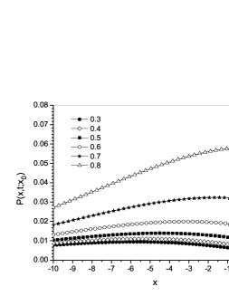
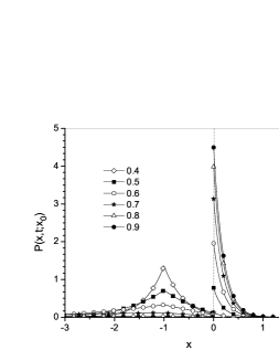
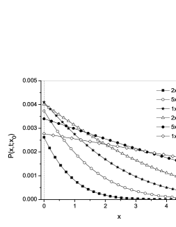
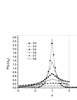
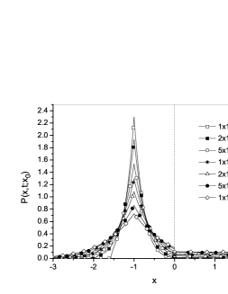
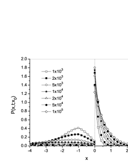
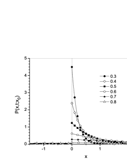
In Figs. 25, the Green’s functions are presented for the system in which the particle is located in the ‘faster’ medium at the initial moment. The calculations were performed taking 20 first terms in the function Eq. (50), and in the series in Eq. (60).
Refer to caption
Figure 2: Plots of the Green’s functions (59) and (60) for various times given in the legend, α1=0.9subscript𝛼10.9\alpha_{1}=0.9, α2=0.5subscript𝛼20.5\alpha_{2}=0.5. The values of the other parameters are D1=D2=0.001subscript𝐷1subscript𝐷20.001D_{1}=D_{2}=0.001, γ~1=0.06subscript~𝛾10.06\tilde{\gamma}_{1}=0.06, γ~2=0.05subscript~𝛾20.05\tilde{\gamma}_{2}=0.05, xN=0subscript𝑥𝑁0x_{N}=0, x0=1subscript𝑥01x_{0}=-1, all quantities are given in arbitrarily chosen units.
Refer to caption
Figure 3: The plots ot the Green’s functions (59) and (60) for various α2subscript𝛼2\alpha_{2} which are given in the legend, α1=0.9subscript𝛼10.9\alpha_{1}=0.9, t=105𝑡superscript105t=10^{5}, the other parameters are the same as in Fig. 2.
Refer to caption
Figure 4: The fragment of Fig. 3 done in the other scale.
Refer to caption
Figure 5: The plots ot the Green’s functions (59) and (60) for various α1subscript𝛼1\alpha_{1} given in the legend, α2=0.3subscript𝛼20.3\alpha_{2}=0.3, t=105𝑡superscript105t=10^{5}, the other parameters are the same as in Fig. 2.

We observe that the concentration in the region x<xN𝑥subscript𝑥𝑁x<x_{N} is similar to the plots occurring in a system with a fully absorbing wall for a sufficiently long time. Namely, in terms of the Laplace transform, the Green’s function for the system with a fully reflecting or fully absorbing wall reads

P^(x,s;x0)=P^H(x,s;x0)+ζP^H(x,s;xs),^𝑃𝑥𝑠subscript𝑥0subscript^𝑃𝐻𝑥𝑠subscript𝑥0𝜁subscript^𝑃𝐻𝑥𝑠subscript𝑥𝑠\hat{P}(x,s;x_{0})=\hat{P}_{H}(x,s;x_{0})+\zeta\hat{P}_{H}(x,s;x_{s})\;, (61)

where xssubscript𝑥𝑠x_{s} is the point located symmetrically to the point x0subscript𝑥0x_{0} with respect to the wall, ζ=1𝜁1\zeta=-1 for the system with an absorbing wall, and ζ=1𝜁1\zeta=1 for the system with a reflecting wall,

P^H(x,s;x0)=s1+α1/22D1e|xx0|sα1/2D1subscript^𝑃𝐻𝑥𝑠subscript𝑥0superscript𝑠1subscript𝛼122subscript𝐷1superscripte𝑥subscript𝑥0superscript𝑠subscript𝛼12subscript𝐷1\hat{P}_{H}(x,s;x_{0})=\frac{s^{-1+\alpha_{1}/2}}{2\sqrt{D_{1}}}{\rm e}^{-\frac{|x-x_{0}|s^{\alpha_{1}/2}}{\sqrt{D_{1}}}} (62)

is the Laplace transform of the Green’s function for a homogeneous system A𝐴A without a wall. The function (57) takes the form of the functions for the system with an absorbing wall under the condition s(2γ~1/γ~2)2/(α1α2)much-less-than𝑠superscript2subscript~𝛾1subscript~𝛾22subscript𝛼1subscript𝛼2s\ll(2\tilde{\gamma}_{1}/\tilde{\gamma}_{2})^{2/(\alpha_{1}-\alpha_{2})}. This inequality provides the condition t(γ~2/2γ~1Γ(1(α1α2)/2))2/(α1α2)much-greater-than𝑡superscriptsubscript~𝛾22subscript~𝛾1Γ1subscript𝛼1subscript𝛼222subscript𝛼1subscript𝛼2t\gg(\tilde{\gamma}_{2}/2\tilde{\gamma}_{1}\Gamma(1-(\alpha_{1}-\alpha_{2})/2))^{2/(\alpha_{1}-\alpha_{2})}.

4.2 From slower to faster region, α1<α2subscript𝛼1subscript𝛼2\alpha_{1}<\alpha_{2}

Let α1<α2subscript𝛼1subscript𝛼2\alpha_{1}<\alpha_{2} and γ~1γ~2subscript~𝛾1subscript~𝛾2\tilde{\gamma}_{1}\neq\tilde{\gamma}_{2}. We transform the functions Λ~A(s)subscript~Λ𝐴𝑠\tilde{\Lambda}_{A}(s) and Λ~B(s)subscript~Λ𝐵𝑠\tilde{\Lambda}_{B}(s), Eqs. (39) and (40), into the following form

Λ~A(s)=1(γ~2/γ~1)s(α2α1)/2+γ~2sα2/21+(γ~2/γ~1)s(α2α1)/2+γ~2sα2/2,subscript~Λ𝐴𝑠1subscript~𝛾2subscript~𝛾1superscript𝑠subscript𝛼2subscript𝛼12subscript~𝛾2superscript𝑠subscript𝛼221subscript~𝛾2subscript~𝛾1superscript𝑠subscript𝛼2subscript𝛼12subscript~𝛾2superscript𝑠subscript𝛼22\tilde{\Lambda}_{A}(s)=\frac{1-(\tilde{\gamma}_{2}/\tilde{\gamma}_{1})s^{(\alpha_{2}-\alpha_{1})/2}+\tilde{\gamma}_{2}s^{\alpha_{2}/2}}{1+(\tilde{\gamma}_{2}/\tilde{\gamma}_{1})s^{(\alpha_{2}-\alpha_{1})/2}+\tilde{\gamma}_{2}s^{\alpha_{2}/2}}\;, (63)
Λ~B(s)=2(γ~2/γ~1)s(α2α1)/21+(γ~2/γ~1)s(α2α1)/2+γ~2sα2/2.subscript~Λ𝐵𝑠2subscript~𝛾2subscript~𝛾1superscript𝑠subscript𝛼2subscript𝛼121subscript~𝛾2subscript~𝛾1superscript𝑠subscript𝛼2subscript𝛼12subscript~𝛾2superscript𝑠subscript𝛼22\tilde{\Lambda}_{B}(s)=\frac{2(\tilde{\gamma}_{2}/\tilde{\gamma}_{1})s^{(\alpha_{2}-\alpha_{1})/2}}{1+(\tilde{\gamma}_{2}/\tilde{\gamma}_{1})s^{(\alpha_{2}-\alpha_{1})/2}+\tilde{\gamma}_{2}s^{\alpha_{2}/2}}\;. (64)

It is convenient for further calculations to transform the Laplace transform of the boundary condition to the following form, which contains the positive values of the exponent of s𝑠s

D2D1γ~2γ~1sα2α1P^A(xN,s;x0)=P^B(xN,s;x0)+γ~2sα2/2P^B(xN,s;x0).subscript𝐷2subscript𝐷1subscript~𝛾2subscript~𝛾1superscript𝑠subscript𝛼2subscript𝛼1subscript^𝑃𝐴subscript𝑥𝑁𝑠subscript𝑥0subscript^𝑃𝐵subscript𝑥𝑁𝑠subscript𝑥0subscript~𝛾2superscript𝑠subscript𝛼22subscript^𝑃𝐵subscript𝑥𝑁𝑠subscript𝑥0\sqrt{\frac{D_{2}}{D_{1}}}\frac{\tilde{\gamma}_{2}}{\tilde{\gamma}_{1}}s^{\alpha_{2}-\alpha_{1}}\hat{P}_{A}(x_{N},s;x_{0})=\hat{P}_{B}(x_{N},s;x_{0})+\tilde{\gamma}_{2}s^{\alpha_{2}/2}\hat{P}_{B}(x_{N},s;x_{0})\;. (65)

The inverse Laplace transform of Eq. (65) reads

D2D1γ~2γ~1α2α1PA(xN,t;x0)tα2α1=PB(xN,t;x0)+γ~2α2/2PB(xN,t;x0)tα2/2.subscript𝐷2subscript𝐷1subscript~𝛾2subscript~𝛾1superscriptsubscript𝛼2subscript𝛼1subscript𝑃𝐴subscript𝑥𝑁𝑡subscript𝑥0superscript𝑡subscript𝛼2subscript𝛼1subscript𝑃𝐵subscript𝑥𝑁𝑡subscript𝑥0subscript~𝛾2superscriptsubscript𝛼22subscript𝑃𝐵subscript𝑥𝑁𝑡subscript𝑥0superscript𝑡subscript𝛼22\sqrt{\frac{D_{2}}{D_{1}}}\frac{\tilde{\gamma}_{2}}{\tilde{\gamma}_{1}}\frac{\partial^{\alpha_{2}-\alpha_{1}}P_{A}(x_{N},t;x_{0})}{\partial t^{\alpha_{2}-\alpha_{1}}}=P_{B}(x_{N},t;x_{0})+\tilde{\gamma}_{2}\frac{\partial^{\alpha_{2}/2}P_{B}(x_{N},t;x_{0})}{\partial t^{\alpha_{2}/2}}\;. (66)

As in the previous case, we consider the Laplace transform of the boundary condition and the Green’s functions in the limit of small values of s𝑠s. For s(1/γ~2)2/α2much-less-than𝑠superscript1subscript~𝛾22subscript𝛼2s\ll\left(1/\tilde{\gamma}_{2}\right)^{2/\alpha_{2}} we can omit the last term on the right–hand side of Eq. (65). Then, for t(γ~2/Γ(1α2/2))2/α2much-greater-than𝑡superscriptsubscript~𝛾2Γ1subscript𝛼222subscript𝛼2t\gg\left(\tilde{\gamma}_{2}/\Gamma(1-\alpha_{2}/2)\right)^{2/\alpha_{2}} the boundary condition reads

PB(xN,t;x0)=D2D1γ~2γ~1α2α1PA(xN,t;x0)tα2α1.subscript𝑃𝐵subscript𝑥𝑁𝑡subscript𝑥0subscript𝐷2subscript𝐷1subscript~𝛾2subscript~𝛾1superscriptsubscript𝛼2subscript𝛼1subscript𝑃𝐴subscript𝑥𝑁𝑡subscript𝑥0superscript𝑡subscript𝛼2subscript𝛼1P_{B}(x_{N},t;x_{0})=\sqrt{\frac{D_{2}}{D_{1}}}\frac{\tilde{\gamma}_{2}}{\tilde{\gamma}_{1}}\frac{\partial^{\alpha_{2}-\alpha_{1}}P_{A}(x_{N},t;x_{0})}{\partial t^{\alpha_{2}-\alpha_{1}}}\;. (67)

We suppose that s(γ~1/γ~2)2/(α2α1)much-less-than𝑠superscriptsubscript~𝛾1subscript~𝛾22subscript𝛼2subscript𝛼1s\ll\left(\tilde{\gamma}_{1}/\tilde{\gamma}_{2}\right)^{2/(\alpha_{2}-\alpha_{1})}. So, we have Λ~A(s)=12(γ~2/γ~1)s(α2α1)/2subscript~Λ𝐴𝑠12subscript~𝛾2subscript~𝛾1superscript𝑠subscript𝛼2subscript𝛼12\tilde{\Lambda}_{A}(s)=1-2(\tilde{\gamma}_{2}/\tilde{\gamma}_{1})s^{(\alpha_{2}-\alpha_{1})/2} and Λ~B(s)=2(γ~2/γ~1)s(α2α1)/2subscript~Λ𝐵𝑠2subscript~𝛾2subscript~𝛾1superscript𝑠subscript𝛼2subscript𝛼12\tilde{\Lambda}_{B}(s)=2(\tilde{\gamma}_{2}/\tilde{\gamma}_{1})s^{(\alpha_{2}-\alpha_{1})/2}. The above functions and Eqs. (37) and (38) provide

P^A(x,s;x0)=s1+α1/22D1[e|xx0|sα1/2D1\displaystyle\hat{P}_{A}(x,s;x_{0})=\frac{s^{-1+\alpha_{1}/2}}{2\sqrt{D_{1}}}\Bigg{[}{\rm e}^{-\frac{|x-x_{0}|s^{\alpha_{1}/2}}{\sqrt{D_{1}}}} (68)
+(12γ~2s(α2α1)/2γ~1)e(2xNxx0)sα1/2D1],\displaystyle+\left(1-\frac{2\tilde{\gamma}_{2}s^{(\alpha_{2}-\alpha_{1})/2}}{\tilde{\gamma}_{1}}\right){\rm e}^{-\frac{(2x_{N}-x-x_{0})s^{\alpha_{1}/2}}{\sqrt{D_{1}}}}\Bigg{]}\;,
P^B(x,s;x0)=γ~2s1+α2α1/2γ~1D2e(xNx0)sα1/2D1e(xxN)sα2/2D2.subscript^𝑃𝐵𝑥𝑠subscript𝑥0subscript~𝛾2superscript𝑠1subscript𝛼2subscript𝛼12subscript~𝛾1subscript𝐷2superscriptesubscript𝑥𝑁subscript𝑥0superscript𝑠subscript𝛼12subscript𝐷1superscripte𝑥subscript𝑥𝑁superscript𝑠subscript𝛼22subscript𝐷2\hat{P}_{B}(x,s;x_{0})=\frac{\tilde{\gamma}_{2}s^{-1+\alpha_{2}-\alpha_{1}/2}}{\tilde{\gamma}_{1}\sqrt{D_{2}}}{\rm e}^{-\frac{(x_{N}-x_{0})s^{\alpha_{1}/2}}{\sqrt{D_{1}}}}{\rm e}^{-\frac{(x-x_{N})s^{\alpha_{2}/2}}{\sqrt{D_{2}}}}\;. (69)

From (50), (68) and (69) we get for tmax[t1,t2]much-greater-than𝑡maxsubscript𝑡1subscript𝑡2t\gg{\rm max}[t_{1},t_{2}], where t1=(γ~2/Γ(1α2/2))2/α2subscript𝑡1superscriptsubscript~𝛾2Γ1subscript𝛼222subscript𝛼2t_{1}=(\tilde{\gamma}_{2}/\Gamma(1-\alpha_{2}/2))^{2/\alpha_{2}}, t2=(γ~2/γ~1Γ(1(α2α1)/2))2/(α2α1)subscript𝑡2superscriptsubscript~𝛾2subscript~𝛾1Γ1subscript𝛼2subscript𝛼122subscript𝛼2subscript𝛼1t_{2}=\left(\tilde{\gamma}_{2}/\tilde{\gamma}_{1}\Gamma(1-(\alpha_{2}-\alpha_{1})/2)\right)^{2/(\alpha_{2}-\alpha_{1})}

PA(x,t;x0)=12D1[f1+α1/2,α1/2(t;|xx0|D1)\displaystyle P_{A}(x,t;x_{0})=\frac{1}{2\sqrt{D_{1}}}\Bigg{[}f_{-1+\alpha_{1}/2,\alpha_{1}/2}\left(t;\frac{|x-x_{0}|}{\sqrt{D_{1}}}\right) (70)
+f1+α1/2,α1/2(t;2xNxx0D1)]\displaystyle+f_{-1+\alpha_{1}/2,\alpha_{1}/2}\left(t;\frac{2x_{N}-x-x_{0}}{\sqrt{D_{1}}}\right)\Bigg{]}
γ~2D1γ~1f1+α2,α1/2(t;2xNxx0D1),subscript~𝛾2subscript𝐷1subscript~𝛾1subscript𝑓1subscript𝛼2subscript𝛼12𝑡2subscript𝑥𝑁𝑥subscript𝑥0subscript𝐷1\displaystyle-\frac{\tilde{\gamma}_{2}}{\sqrt{D_{1}}\tilde{\gamma}_{1}}f_{-1+\alpha_{2},\alpha_{1}/2}\left(t;\frac{2x_{N}-x-x_{0}}{\sqrt{D_{1}}}\right)\;,
PB(x,t;x0)=γ~2D2γ~1n=01n!(xNxD2)nsubscript𝑃𝐵𝑥𝑡subscript𝑥0subscript~𝛾2subscript𝐷2subscript~𝛾1superscriptsubscript𝑛01𝑛superscriptsubscript𝑥𝑁𝑥subscript𝐷2𝑛\displaystyle P_{B}(x,t;x_{0})=\frac{\tilde{\gamma}_{2}}{\sqrt{D_{2}}\tilde{\gamma}_{1}}\sum_{n=0}^{\infty}\frac{1}{n!}\left(\frac{x_{N}-x}{\sqrt{D_{2}}}\right)^{n} (71)
×f1α1/2+α2(1+n/2),α1/2(t;xNx0D1).absentsubscript𝑓1subscript𝛼12subscript𝛼21𝑛2subscript𝛼12𝑡subscript𝑥𝑁subscript𝑥0subscript𝐷1\displaystyle\times f_{-1-\alpha_{1}/2+\alpha_{2}(1+n/2),\alpha_{1}/2}\left(t;\frac{x_{N}-x_{0}}{\sqrt{D_{1}}}\right)\;.
Refer to caption
Figure 6: The plots of the Green’s functions (70) and (71) for various time given in the legend, α1=0.5subscript𝛼10.5\alpha_{1}=0.5, α2=0.9subscript𝛼20.9\alpha_{2}=0.9, the other parameters are the same as in Fig. 2.
Refer to caption
Figure 7: The fragment of Fig. 6 presented in the other scale of space variable.
Refer to caption
Figure 8: The plots ot the Green’s functions (70) and (71) for various α1subscript𝛼1\alpha_{1} which are given in the legend, α2=0.9subscript𝛼20.9\alpha_{2}=0.9, t=105𝑡superscript105t=10^{5}, the other parameters are the same as in Fig. 2.

We observe that the concentration in the region x<xN𝑥subscript𝑥𝑁x<x_{N} is similar to the plots occurring in a system with a fully reflecting wall for sufficiently long times. The function (68) takes the form of the functions for the system with a reflecting wall under condition s(2γ~2/γ~1)2/(α2α1)much-less-than𝑠superscript2subscript~𝛾2subscript~𝛾12subscript𝛼2subscript𝛼1s\ll(2\tilde{\gamma}_{2}/\tilde{\gamma}_{1})^{2/(\alpha_{2}-\alpha_{1})}. This equality provides the condition t(γ~1/2γ~2Γ(1(α2α1)/2))2/(α2α1)much-greater-than𝑡superscriptsubscript~𝛾12subscript~𝛾2Γ1subscript𝛼2subscript𝛼122subscript𝛼2subscript𝛼1t\gg(\tilde{\gamma}_{1}/2\tilde{\gamma}_{2}\Gamma(1-(\alpha_{2}-\alpha_{1})/2))^{2/(\alpha_{2}-\alpha_{1})}.

4.3 The case of α1=α2subscript𝛼1subscript𝛼2\alpha_{1}=\alpha_{2}

Let α1=α2=αsubscript𝛼1subscript𝛼2𝛼\alpha_{1}=\alpha_{2}=\alpha. The functions Λ~A(s)subscript~Λ𝐴𝑠\tilde{\Lambda}_{A}(s) and Λ~B(s)subscript~Λ𝐵𝑠\tilde{\Lambda}_{B}(s) take the following form

Λ~A(s)=γ~1γ~2+γ~1γ~2sα/2γ~1+γ~2+γ~1γ~2sα/2,subscript~Λ𝐴𝑠subscript~𝛾1subscript~𝛾2subscript~𝛾1subscript~𝛾2superscript𝑠𝛼2subscript~𝛾1subscript~𝛾2subscript~𝛾1subscript~𝛾2superscript𝑠𝛼2\tilde{\Lambda}_{A}(s)=\frac{\tilde{\gamma}_{1}-\tilde{\gamma}_{2}+\tilde{\gamma}_{1}\tilde{\gamma}_{2}s^{\alpha/2}}{\tilde{\gamma}_{1}+\tilde{\gamma}_{2}+\tilde{\gamma}_{1}\tilde{\gamma}_{2}s^{\alpha/2}}\;, (72)
Λ~B(s)=2γ~1+γ~2+γ~1γ~2sα/2.subscript~Λ𝐵𝑠2subscript~𝛾1subscript~𝛾2subscript~𝛾1subscript~𝛾2superscript𝑠𝛼2\tilde{\Lambda}_{B}(s)=\frac{2}{\tilde{\gamma}_{1}+\tilde{\gamma}_{2}+\tilde{\gamma}_{1}\tilde{\gamma}_{2}s^{\alpha/2}}\;. (73)

In terms of the Laplace transform the boundary condition Eq. (42) is the following

P^A(xN,s;x0)=D2D1[γ~1γ~2+γ~1sα/2]P^B(xN,s;x0).subscript^𝑃𝐴subscript𝑥𝑁𝑠subscript𝑥0subscript𝐷2subscript𝐷1delimited-[]subscript~𝛾1subscript~𝛾2subscript~𝛾1superscript𝑠𝛼2subscript^𝑃𝐵subscript𝑥𝑁𝑠subscript𝑥0\displaystyle\hat{P}_{A}(x_{N},s;x_{0})=\sqrt{\frac{D_{2}}{D_{1}}}\left[\frac{\tilde{\gamma}_{1}}{\tilde{\gamma}_{2}}+\tilde{\gamma}_{1}s^{\alpha/2}\right]\hat{P}_{B}(x_{N},s;x_{0})\;. (74)

The inverse Laplace transform of Eq. (74) reads

PA(xN,t;x0)=D2D1γ~1γ~2PB(xN,t;x0)+D2D1γ~1α/2PB(xN,t;x0)tα/2.subscript𝑃𝐴subscript𝑥𝑁𝑡subscript𝑥0subscript𝐷2subscript𝐷1subscript~𝛾1subscript~𝛾2subscript𝑃𝐵subscript𝑥𝑁𝑡subscript𝑥0subscript𝐷2subscript𝐷1subscript~𝛾1superscript𝛼2subscript𝑃𝐵subscript𝑥𝑁𝑡subscript𝑥0superscript𝑡𝛼2P_{A}(x_{N},t;x_{0})=\sqrt{\frac{D_{2}}{D_{1}}}\frac{\tilde{\gamma}_{1}}{\tilde{\gamma}_{2}}P_{B}(x_{N},t;x_{0})+\sqrt{\frac{D_{2}}{D_{1}}}\tilde{\gamma}_{1}\frac{\partial^{\alpha/2}P_{B}(x_{N},t;x_{0})}{\partial t^{\alpha/2}}\;. (75)

In the limit of small s𝑠s, s(1/γ~2)2/αmuch-less-than𝑠superscript1subscript~𝛾22𝛼s\ll\left(1/\tilde{\gamma}_{2}\right)^{2/\alpha}, the Laplace transform of boundary condition (74) reads

P^A(xN,s;x0)=D2D1γ~1γ~2P^B(xN,s;x0).subscript^𝑃𝐴subscript𝑥𝑁𝑠subscript𝑥0subscript𝐷2subscript𝐷1subscript~𝛾1subscript~𝛾2subscript^𝑃𝐵subscript𝑥𝑁𝑠subscript𝑥0\hat{P}_{A}(x_{N},s;x_{0})=\sqrt{\frac{D_{2}}{D_{1}}}\frac{\tilde{\gamma}_{1}}{\tilde{\gamma}_{2}}\hat{P}_{B}(x_{N},s;x_{0})\;. (76)

The inverse Laplace transform of Eq. (76) is the following

PA(xN,t;x0)=D2D1γ~1γ~2PB(xN,t;x0).subscript𝑃𝐴subscript𝑥𝑁𝑡subscript𝑥0subscript𝐷2subscript𝐷1subscript~𝛾1subscript~𝛾2subscript𝑃𝐵subscript𝑥𝑁𝑡subscript𝑥0P_{A}(x_{N},t;x_{0})=\sqrt{\frac{D_{2}}{D_{1}}}\frac{\tilde{\gamma}_{1}}{\tilde{\gamma}_{2}}P_{B}(x_{N},t;x_{0})\;. (77)

Assuming additionally: s(γ~1γ~2/(γ~1+γ~2))2/αmuch-less-than𝑠superscriptsubscript~𝛾1subscript~𝛾2subscript~𝛾1subscript~𝛾22𝛼s\ll\left(\tilde{\gamma}_{1}\tilde{\gamma}_{2}/(\tilde{\gamma}_{1}+\tilde{\gamma}_{2})\right)^{2/\alpha}, from Eqs. (72) and (73) we obtain

Λ~A(s)=κ~1+κ~2sα/2,subscript~Λ𝐴𝑠subscript~𝜅1subscript~𝜅2superscript𝑠𝛼2\tilde{\Lambda}_{A}(s)=\tilde{\kappa}_{1}+\tilde{\kappa}_{2}s^{\alpha/2}\;, (78)
Λ~B(s)=1κ~1κ~2sα/2,subscript~Λ𝐵𝑠1subscript~𝜅1subscript~𝜅2superscript𝑠𝛼2\tilde{\Lambda}_{B}(s)=1-\tilde{\kappa}_{1}-\tilde{\kappa}_{2}s^{\alpha/2}\;, (79)

where

κ~1=γ~1γ~2γ~1+γ~2,κ~2=2γ~1γ~22(γ~1+γ~2)2.formulae-sequencesubscript~𝜅1subscript~𝛾1subscript~𝛾2subscript~𝛾1subscript~𝛾2subscript~𝜅22subscript~𝛾1subscriptsuperscript~𝛾22superscriptsubscript~𝛾1subscript~𝛾22\tilde{\kappa}_{1}=\frac{\tilde{\gamma}_{1}-\tilde{\gamma}_{2}}{\tilde{\gamma}_{1}+\tilde{\gamma}_{2}}\;,\;\tilde{\kappa}_{2}=\frac{2\tilde{\gamma}_{1}\tilde{\gamma}^{2}_{2}}{(\tilde{\gamma}_{1}+\tilde{\gamma}_{2})^{2}}\;. (80)

The inverse formulae to Eq. (80) are γ~1=2κ~2/(1κ~1)2subscript~𝛾12subscript~𝜅2superscript1subscript~𝜅12\tilde{\gamma}_{1}=2\tilde{\kappa}_{2}/(1-\tilde{\kappa}_{1})^{2} and γ~2=2κ~2/(1κ~22)subscript~𝛾22subscript~𝜅21superscriptsubscript~𝜅22\tilde{\gamma}_{2}=2\tilde{\kappa}_{2}/(1-\tilde{\kappa}_{2}^{2}). Taking into account Eqs. (78) and (79) we obtain

P^A(x,t;x0)=s1+α/22D1[e|xx0|sα/2D1+(κ~1+κ~2sα/2)e(2xNxx0)sα/2D1],subscript^𝑃𝐴𝑥𝑡subscript𝑥0superscript𝑠1𝛼22subscript𝐷1delimited-[]superscripte𝑥subscript𝑥0superscript𝑠𝛼2subscript𝐷1subscript~𝜅1subscript~𝜅2superscript𝑠𝛼2superscripte2subscript𝑥𝑁𝑥subscript𝑥0superscript𝑠𝛼2subscript𝐷1\hat{P}_{A}(x,t;x_{0})=\frac{s^{-1+\alpha/2}}{2\sqrt{D_{1}}}\Bigg{[}{\rm e}^{-\frac{|x-x_{0}|s^{\alpha/2}}{\sqrt{D_{1}}}}+\left(\tilde{\kappa}_{1}+\tilde{\kappa}_{2}s^{\alpha/2}\right){\rm e}^{-\frac{(2x_{N}-x-x_{0})s^{\alpha/2}}{\sqrt{D_{1}}}}\Bigg{]}\;, (81)
P^B(x,t;x0)=s1+α/22D2(1κ~1κ~2sα/2)e(xNx0)sα/2D1e(xxN)sα/2D2.subscript^𝑃𝐵𝑥𝑡subscript𝑥0superscript𝑠1𝛼22subscript𝐷21subscript~𝜅1subscript~𝜅2superscript𝑠𝛼2superscriptesubscript𝑥𝑁subscript𝑥0superscript𝑠𝛼2subscript𝐷1superscripte𝑥subscript𝑥𝑁superscript𝑠𝛼2subscript𝐷2\hat{P}_{B}(x,t;x_{0})=\frac{s^{-1+\alpha/2}}{2\sqrt{D_{2}}}\left(1-\tilde{\kappa}_{1}-\tilde{\kappa}_{2}s^{\alpha/2}\right){\rm e}^{-\frac{(x_{N}-x_{0})s^{\alpha/2}}{\sqrt{D_{1}}}}{\rm e}^{-\frac{(x-x_{N})s^{\alpha/2}}{\sqrt{D_{2}}}}\;. (82)
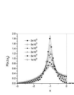
Refer to caption
Figure 9: The plots ot the Green’s functions (83) and (84) for various times which are given in the legend, α1=α2=0.5subscript𝛼1subscript𝛼20.5\alpha_{1}=\alpha_{2}=0.5, D1=0.001subscript𝐷10.001D_{1}=0.001, D2=0.002subscript𝐷20.002D_{2}=0.002, γ~1=0.06subscript~𝛾10.06\tilde{\gamma}_{1}=0.06, γ~2=0.05subscript~𝛾20.05\tilde{\gamma}_{2}=0.05, x0=1subscript𝑥01x_{0}=-1, and xN=0subscript𝑥𝑁0x_{N}=0.

The inverse Laplace transform of Eqs. (81) and (82) reads for t((γ~1+γ~2)/γ~1γ~2Γ(1α/2))2/αmuch-greater-than𝑡superscriptsubscript~𝛾1subscript~𝛾2subscript~𝛾1subscript~𝛾2Γ1𝛼22𝛼t\gg\left((\tilde{\gamma}_{1}+\tilde{\gamma}_{2})/\tilde{\gamma}_{1}\tilde{\gamma}_{2}\Gamma(1-\alpha/2)\right)^{2/\alpha}

PA(x,t;x0)=12D1[f1+α/2,α/2(t;|xx0|D1)\displaystyle P_{A}(x,t;x_{0})=\frac{1}{2\sqrt{D_{1}}}\Bigg{[}f_{-1+\alpha/2,\alpha/2}\left(t;\frac{|x-x_{0}|}{\sqrt{D_{1}}}\right) (83)
+κ~1f1+α/2,α/2(t;2xNxx0D1)subscript~𝜅1subscript𝑓1𝛼2𝛼2𝑡2subscript𝑥𝑁𝑥subscript𝑥0subscript𝐷1\displaystyle+\tilde{\kappa}_{1}f_{-1+\alpha/2,\alpha/2}\left(t;\frac{2x_{N}-x-x_{0}}{\sqrt{D_{1}}}\right)
+κ~2f1+α,α/2(t;2xNxx0D1)],\displaystyle+\tilde{\kappa}_{2}f_{-1+\alpha,\alpha/2}\left(t;\frac{2x_{N}-x-x_{0}}{\sqrt{D_{1}}}\right)\Bigg{]}\;,
PB(x,t;x0)=12D2n=01n!(xNxD2)nsubscript𝑃𝐵𝑥𝑡subscript𝑥012subscript𝐷2superscriptsubscript𝑛01𝑛superscriptsubscript𝑥𝑁𝑥subscript𝐷2𝑛\displaystyle P_{B}(x,t;x_{0})=\frac{1}{2\sqrt{D_{2}}}\sum_{n=0}^{\infty}\frac{1}{n!}\left(\frac{x_{N}-x}{\sqrt{D_{2}}}\right)^{n} (84)
×[(1κ~1)f1+α(1+n/2),α1/2(t;xNx0D1)\displaystyle\times\Big{[}(1-\tilde{\kappa}_{1})f_{-1+\alpha(1+n/2),\alpha_{1}/2}\left(t;\frac{x_{N}-x_{0}}{\sqrt{D_{1}}}\right)
κ~2f1+α(3+n)/2,α/2(t;xNx0D1)].\displaystyle-\tilde{\kappa}_{2}f_{-1+\alpha(3+n)/2,\alpha/2}\left(t;\frac{x_{N}-x_{0}}{\sqrt{D_{1}}}\right)\Big{]}\;.

In this case the plots of Green’s functions are qualitatively similar to the ones obtained for the system in which a membrane is located in a homogeneous medium, see [24]. In contrast to the case of α1α2subscript𝛼1subscript𝛼2\alpha_{1}\neq\alpha_{2}, we do not observe any Green’s function characteristic of a system with an absorbing or reflecting wall.

5 Final remarks

The main results presented in this paper are both the Green’s functions, Eqs. (37) and (38), and boundary conditions at a thin membrane, Eqs. (42) and (48), given in terms of the Laplace transform. From these equations we can derive both Green’s functions and boundary conditions at the membrane in time domain, over a limit of long time, for various relations between the subdiffusion parameters α1subscript𝛼1\alpha_{1} and α2subscript𝛼2\alpha_{2}. The examples for the calculation of the Green’s functions and the boundary conditions from their Laplace transforms are shown in Sec. 4. The boundary conditions at a thin membrane can be used to calculate particles’ concentration profiles in systems consisting of many parts separated by thin membranes, including the case of subdiffusion in a system with a thick membrane.

In this paper we also present the new method of deriving the Green’s function for a system in which two different media are separated by a thin partially permeable membrane. Within this method we first consider a particle’s random walk in a system with a discrete time and space variable in which the particle may vanish due to reactions with constant probabilities defined separately for each medium. The reactions fulfil the supporting role. Since we link the reaction parameters to subdiffusion parameters, the presence of reactions allow us to include the subdiffusion parameters of both media into the Green’s functions derived from a random walk model. So, we move from discrete to continuous variables in the obtained formulae and eliminate the reactions. Finally, we obtained the Green’s functions for the system without reactions. The functions obtained were used to determine the boundary conditions at the thin membrane. The results presented in this paper are also valid when normal diffusion occurs in the system. We obtain the Green’s functions and boundary conditions for a normal diffusion case by placing α1=1subscript𝛼11\alpha_{1}=1 and/or α2=1subscript𝛼21\alpha_{2}=1 into the obtained formulae.

The model based on the random walk model with a discrete time and space variable seems to be oversimplified. However, it provides somewhat nontrivial results which have a simple physical interpretation. We add that such models were used to model subdiffusion processes in membrane systems [24, 25], as was mentionad earlier in this paper, as well as in the system with reactions [48, 50].

The Green’s functions differ qualitatively depending on whether a particle starts its subdiffusive random walk from a faster or slower medium, which is shown in Figs. 27. If the particle starts from a ‘faster’ medium, then its random walk in this medium is performed just as in the medium with an absorbing membrane, whereas when the particle starts from a ‘slower’ medium, then its random walk in this medium is similar to subdiffusion occurring in a system with a reflecting membrane over a long time limit. In both cases, the probability of finding the particle in the ‘slower’ medium significantly increases over time.

We have considered the process in which x0<xNsubscript𝑥0subscript𝑥𝑁x_{0}<x_{N}. The Green’s functions obtained in this paper can be easily transformed for the case of x0>xNsubscript𝑥0subscript𝑥𝑁x_{0}>x_{N} using the symmetry argument, which, in practice, means that the following conversion is made: α1α2subscript𝛼1subscript𝛼2\alpha_{1}\longrightarrow\alpha_{2}, α2α1subscript𝛼2subscript𝛼1\alpha_{2}\longrightarrow\alpha_{1}, D1D2subscript𝐷1subscript𝐷2D_{1}\longrightarrow D_{2}, D2D1subscript𝐷2subscript𝐷1D_{2}\longrightarrow D_{1}, γ~1γ~2subscript~𝛾1subscript~𝛾2\tilde{\gamma}_{1}\longrightarrow\tilde{\gamma}_{2}, γ~2γ~1subscript~𝛾2subscript~𝛾1\tilde{\gamma}_{2}\longrightarrow\tilde{\gamma}_{1}, xx0x0x𝑥subscript𝑥0subscript𝑥0𝑥x-x_{0}\longrightarrow x_{0}-x, xxNxNx𝑥subscript𝑥𝑁subscript𝑥𝑁𝑥x-x_{N}\longrightarrow x_{N}-x, and xNx0x0xNsubscript𝑥𝑁subscript𝑥0subscript𝑥0subscript𝑥𝑁x_{N}-x_{0}\longrightarrow x_{0}-x_{N}. If we consider a system with many particles and if the particles move independently of each other, the concentration of particles C(x,t)𝐶𝑥𝑡C(x,t) can be calculated by means of the following formula C(x,t)=P(x,t;x0)C(x0,0)𝑑x0𝐶𝑥𝑡superscriptsubscript𝑃𝑥𝑡subscript𝑥0𝐶subscript𝑥00differential-dsubscript𝑥0C(x,t)=\int_{-\infty}^{\infty}P(x,t;x_{0})C(x_{0},0)dx_{0}. The procedure of finding the concentration profiles for the arbitrarily chosen initial condition C(x0,0)𝐶subscript𝑥00C(x_{0},0) is identical to the procedure described in [24] (see Eqs. (78)–(90) in the above cited paper), where subdiffusion in a system in which a thin membrane separates two identical media is taken into account.

The results presented in this paper agree in part with the results obtained in [26, 27, 28], in which subdiffusion in a system which consists of two different subdiffusive media are joined at point xNsubscript𝑥𝑁x_{N}. However, in these papers, only the Green’s function for the case of x0=xNsubscript𝑥0subscript𝑥𝑁x_{0}=x_{N} was found. The Laplace transforms of the Green’s functions derived in the above cited paper coincides with Eqs. (57), (58) and Eqs. (68), (69) presented in this paper, only in the case of x0=xNsubscript𝑥0subscript𝑥𝑁x_{0}=x_{N}. The boundary condition derived in [28] coincides with boundary conditions Eqs. (56) and (67) in this paper which are the approximation of more general boundary conditions, Eqs. (4.1) and (66), respectively, over a long time limit. The model presented in this paper allows us to consider the subdiffusion of a particle initially located at an arbitrarily chosen point x0subscript𝑥0x_{0}.

Below, we add the comments concerning the technical aspects of the calculations. The moving from a discrete to continuous spatial variable is interpreted slightly differently from mathematical or physical points of view. Mathematically, this moving consists of calculating the limit ϵ0italic-ϵ0\epsilon\longrightarrow 0 in the Green’s functions already obtained for a discrete spatial variable. Physically, supposing that ϵitalic-ϵ\epsilon is very small but finite, one may expand the Green’s functions in the series with respect to ϵitalic-ϵ\epsilon and then omit the terms of the order equal to or larger than 1 with respect to ϵitalic-ϵ\epsilon. The difference between both approaches is caused by the fact that in the limit ϵ0italic-ϵ0\epsilon\longrightarrow 0, the probability distribution ω(t)𝜔𝑡\omega(t) of the waiting time for a particle to take its next step loses its physical interpretation; this problem is briefly discussed just below Eq. (33). However, these two approaches lead to the same result; so, in practice, it is possible to use both in order to find the functions for a continuous spatial variable.

One of the criteria that provides the utility of the used approximation is that the Green’s functions obtained for a membrane system should depend on the parameters of membrane permeability including the case of γ~1=γ~2subscript~𝛾1subscript~𝛾2\tilde{\gamma}_{1}=\tilde{\gamma}_{2} (see the discussion presented in [24]). However, when α1α2subscript𝛼1subscript𝛼2\alpha_{1}\neq\alpha_{2}, several leading terms in the series which approximate the functions (39) and (40) with respect to s𝑠s, are dependent on the ratio γ~1/γ~2subscript~𝛾1subscript~𝛾2\tilde{\gamma}_{1}/\tilde{\gamma}_{2} alone; the number of leading terms increases when |α1α2|subscript𝛼1subscript𝛼2|\alpha_{1}-\alpha_{2}| becomes smaller. When γ~1=γ~2subscript~𝛾1subscript~𝛾2\tilde{\gamma}_{1}=\tilde{\gamma}_{2}, in order to include the membrane permeability parameters in the approximate Green’s functions, we have to include a relatively large number of terms, especially when α1α2subscript𝛼1subscript𝛼2\alpha_{1}\neq\alpha_{2} and |α1α2|1much-less-thansubscript𝛼1subscript𝛼21|\alpha_{1}-\alpha_{2}|\ll 1. We note that this problem does not occur in the system with α1=α2subscript𝛼1subscript𝛼2\alpha_{1}=\alpha_{2}. In this paper, we consider the subdiffusion in the composite membrane system for the case of α1α2subscript𝛼1subscript𝛼2\alpha_{1}\neq\alpha_{2}, assuming γ~1γ~2subscript~𝛾1subscript~𝛾2\tilde{\gamma}_{1}\neq\tilde{\gamma}_{2}. We presume that the last condition is not significantly limiting in our considerations. Although from the mathematical point of view, the cases γ~1=γ~2subscript~𝛾1subscript~𝛾2\tilde{\gamma}_{1}=\tilde{\gamma}_{2} and γ~1γ~2subscript~𝛾1subscript~𝛾2\tilde{\gamma}_{1}\neq\tilde{\gamma}_{2} should be treated ‘equitably’, from the physical point of view, the case of γ~1γ~2subscript~𝛾1subscript~𝛾2\tilde{\gamma}_{1}\neq\tilde{\gamma}_{2} is preferable. The case of γ~1=γ~2subscript~𝛾1subscript~𝛾2\tilde{\gamma}_{1}=\tilde{\gamma}_{2} naturally occurs when a symmetrical thin membrane is located in a homogeneous system in which α1=α2subscript𝛼1subscript𝛼2\alpha_{1}=\alpha_{2}. The Green’s functions for such a system are a special case of the functions obtained in Sec. IIIC. For the system in which α1α2subscript𝛼1subscript𝛼2\alpha_{1}\neq\alpha_{2}, the coefficients γ~1=γ1/D1subscript~𝛾1subscript𝛾1subscript𝐷1\tilde{\gamma}_{1}=\gamma_{1}/\sqrt{D_{1}} and γ~2=γ2/D2subscript~𝛾2subscript𝛾2subscript𝐷2\tilde{\gamma}_{2}=\gamma_{2}/\sqrt{D_{2}}, which are given in different physical units, are equal for a very particular combination of parameters which reads D1/D2=(γ1/γ2)2subscript𝐷1subscript𝐷2superscriptsubscript𝛾1subscript𝛾22D_{1}/D_{2}=\left(\gamma_{1}/\gamma_{2}\right)^{2}. We note that γisubscript𝛾𝑖\gamma_{i} is measured in the units m𝑚m, whereas Disubscript𝐷𝑖D_{i} is measured in units m2/sαisuperscript𝑚2superscript𝑠subscript𝛼𝑖m^{2}/s^{\alpha_{i}}, i=1,2𝑖12i=1,2. Changing the units of time provides a change on the left–hand side of the above relation, with its right–hand side remaining unchanged. Thus, the assumption γ~1γ~2subscript~𝛾1subscript~𝛾2\tilde{\gamma}_{1}\neq\tilde{\gamma}_{2} seems to have a good basis for the case of α1α2subscript𝛼1subscript𝛼2\alpha_{1}\neq\alpha_{2}.

Acknowledgments

The author would like to thank Dr. Katarzyna D. Lewandowska for her helpful discussions. This paper was partially supported by the Polish National Science Centre under grant No. 2014/13/D/ST2/03608.

Appendix I

We show the method of calculating the functions Eqs. (10)–(14). Using Eqs. (2.1)–(9), we obtain

1z[SA(m,z;m0)δm,m0]=12SA(m1,z;m0)+12SA(m+1,z;m0)1𝑧delimited-[]subscript𝑆𝐴𝑚𝑧subscript𝑚0subscript𝛿𝑚subscript𝑚012subscript𝑆𝐴𝑚1𝑧subscript𝑚012subscript𝑆𝐴𝑚1𝑧subscript𝑚0\displaystyle\frac{1}{z}\left[S_{A}(m,z;m_{0})-\delta_{m,m_{0}}\right]=\frac{1}{2}S_{A}(m-1,z;m_{0})+\frac{1}{2}S_{A}(m+1,z;m_{0})
R1SA(m,z;m0)mN,N+1,formulae-sequencesubscript𝑅1subscript𝑆𝐴𝑚𝑧subscript𝑚0𝑚𝑁𝑁1\displaystyle-R_{1}S_{A}(m,z;m_{0})\qquad m\neq N,N+1\;, (85)
1z[SA(N,z;m0)δN,m0]=12SA(N1,z;m0)+1q22SB(N+1,z;m0)1𝑧delimited-[]subscript𝑆𝐴𝑁𝑧subscript𝑚0subscript𝛿𝑁subscript𝑚012subscript𝑆𝐴𝑁1𝑧subscript𝑚01subscript𝑞22subscript𝑆𝐵𝑁1𝑧subscript𝑚0\displaystyle\frac{1}{z}\left[S_{A}(N,z;m_{0})-\delta_{N,m_{0}}\right]=\frac{1}{2}S_{A}(N-1,z;m_{0})+\frac{1-q_{2}}{2}S_{B}(N+1,z;m_{0})
+1q12SA(N+1,z;m0)R1SA(N,z;m0),1subscript𝑞12subscript𝑆𝐴𝑁1𝑧subscript𝑚0subscript𝑅1subscript𝑆𝐴𝑁𝑧subscript𝑚0\displaystyle+\frac{1-q_{1}}{2}S_{A}(N+1,z;m_{0})-R_{1}S_{A}(N,z;m_{0})\;, (86)
1z[SB(N+1,z;m0)δN+1,m0]=1q12SA(N,z;m0)+12SB(N+2,z;m0)1𝑧delimited-[]subscript𝑆𝐵𝑁1𝑧subscript𝑚0subscript𝛿𝑁1subscript𝑚01subscript𝑞12subscript𝑆𝐴𝑁𝑧subscript𝑚012subscript𝑆𝐵𝑁2𝑧subscript𝑚0\displaystyle\frac{1}{z}\left[S_{B}(N+1,z;m_{0})-\delta_{N+1,m_{0}}\right]=\frac{1-q_{1}}{2}S_{A}(N,z;m_{0})+\frac{1}{2}S_{B}(N+2,z;m_{0})
+q22SB(N+1,z;m0)R2SB(N+1,z;m0),subscript𝑞22subscript𝑆𝐵𝑁1𝑧subscript𝑚0subscript𝑅2subscript𝑆𝐵𝑁1𝑧subscript𝑚0\displaystyle+\frac{q_{2}}{2}S_{B}(N+1,z;m_{0})-R_{2}S_{B}(N+1,z;m_{0})\;, (87)
1z[SB(m,z;m0)δm,m0]=12SB(m1,z;m0)+12SB(m+1,z;m0)1𝑧delimited-[]subscript𝑆𝐵𝑚𝑧subscript𝑚0subscript𝛿𝑚subscript𝑚012subscript𝑆𝐵𝑚1𝑧subscript𝑚012subscript𝑆𝐵𝑚1𝑧subscript𝑚0\displaystyle\frac{1}{z}\left[S_{B}(m,z;m_{0})-\delta_{m,m_{0}}\right]=\frac{1}{2}S_{B}(m-1,z;m_{0})+\frac{1}{2}S_{B}(m+1,z;m_{0})
R2SB(m,z;m0),m>N+1.subscript𝑅2subscript𝑆𝐵𝑚𝑧subscript𝑚0𝑚𝑁1\displaystyle-R_{2}S_{B}(m,z;m_{0})\;,\qquad m>N+1\;. (88)

In order to solve Eqs. (Appendix I)–(Appendix I), we use the following generating functions with respect to the space variable

GA(u,z;m0)=m=NumSA(m,z;m0),subscript𝐺𝐴𝑢𝑧subscript𝑚0superscriptsubscript𝑚𝑁superscript𝑢𝑚subscript𝑆𝐴𝑚𝑧subscript𝑚0\displaystyle G_{A}(u,z;m_{0})=\sum_{m=-\infty}^{N}u^{m}S_{A}(m,z;m_{0})\;, (89)
GB(u,z;m0)=m=N+1umSB(m,z;m0).subscript𝐺𝐵𝑢𝑧subscript𝑚0superscriptsubscript𝑚𝑁1superscript𝑢𝑚subscript𝑆𝐵𝑚𝑧subscript𝑚0\displaystyle G_{B}(u,z;m_{0})=\sum_{m=N+1}^{\infty}u^{m}S_{B}(m,z;m_{0})\;. (90)

After calculating, we obtain

GA(u,z;m0)[1z2(u+1u+R1z)]subscript𝐺𝐴𝑢𝑧subscript𝑚0delimited-[]1𝑧2𝑢1𝑢subscript𝑅1𝑧\displaystyle G_{A}(u,z;m_{0})\left[1-\frac{z}{2}\left(u+\frac{1}{u}+R_{1}z\right)\right] (91)
=z2uN[q1SA(N,z;m0)+(1q2)SB(N+1,z;m0)]absent𝑧2superscript𝑢𝑁delimited-[]subscript𝑞1subscript𝑆𝐴𝑁𝑧subscript𝑚01subscript𝑞2subscript𝑆𝐵𝑁1𝑧subscript𝑚0\displaystyle=\frac{z}{2}u^{N}\left[q_{1}S_{A}(N,z;m_{0})+(1-q_{2})S_{B}(N+1,z;m_{0})\right]
+um0z2uN+1SA(N,z;m0),superscript𝑢subscript𝑚0𝑧2superscript𝑢𝑁1subscript𝑆𝐴𝑁𝑧subscript𝑚0\displaystyle+u^{m_{0}}-\frac{z}{2}u^{N+1}S_{A}(N,z;m_{0})\;,
GB(u,z;m0)[1z2(u+1u+R2z)]subscript𝐺𝐵𝑢𝑧subscript𝑚0delimited-[]1𝑧2𝑢1𝑢subscript𝑅2𝑧\displaystyle G_{B}(u,z;m_{0})\left[1-\frac{z}{2}\left(u+\frac{1}{u}+R_{2}z\right)\right] (92)
=z2uN+1[(1q1)SA(N,z;m0)+q2SB(N+1,z;m0)]absent𝑧2superscript𝑢𝑁1delimited-[]1subscript𝑞1subscript𝑆𝐴𝑁𝑧subscript𝑚0subscript𝑞2subscript𝑆𝐵𝑁1𝑧subscript𝑚0\displaystyle=\frac{z}{2}u^{N+1}\left[(1-q_{1})S_{A}(N,z;m_{0})+q_{2}S_{B}(N+1,z;m_{0})\right]
z2uNSB(N+1,z;m0).𝑧2superscript𝑢𝑁subscript𝑆𝐵𝑁1𝑧subscript𝑚0\displaystyle-\frac{z}{2}u^{N}S_{B}(N+1,z;m_{0})\;.

The generating function Sisubscript𝑆𝑖S_{i} can be obtained by means of the following formula

Si(m,z;m0)=12πiK(𝟎,1)Gi(u,z;m0)um+1𝑑u,subscript𝑆𝑖𝑚𝑧subscript𝑚012𝜋𝑖subscriptcontour-integral𝐾01subscript𝐺𝑖𝑢𝑧subscript𝑚0superscript𝑢𝑚1differential-d𝑢S_{i}(m,z;m_{0})=\frac{1}{2\pi i}\oint_{K({\bf 0},1)}\frac{G_{i}(u,z;m_{0})}{u^{m+1}}du\;, (93)

where i=A,B𝑖𝐴𝐵i=A,B, the integration is carried out along the unit circle K𝐾K centered at the point 𝟎=(0,0)000{\bf 0}=(0,0) to be consistent with the increasing argument of a complex number. Using the integral formula

12πiK(𝟎,1)um0um+1[1z2(u+1u)+zR]𝑑u12𝜋𝑖subscriptcontour-integral𝐾01superscript𝑢subscript𝑚0superscript𝑢𝑚1delimited-[]1𝑧2𝑢1𝑢𝑧𝑅differential-d𝑢\displaystyle\frac{1}{2\pi i}\oint_{K({\bf 0},1)}\frac{u^{m_{0}}}{u^{m+1}\left[1-\frac{z}{2}\left(u+\frac{1}{u}\right)+zR\right]}du (94)
=(1+zR(1+zR)2z2z)|mm0|1(1+zR)2z2,absentsuperscript1𝑧𝑅superscript1𝑧𝑅2superscript𝑧2𝑧𝑚subscript𝑚01superscript1𝑧𝑅2superscript𝑧2\displaystyle=\left(\frac{1+zR-\sqrt{(1+zR)^{2}-z^{2}}}{z}\right)^{|m-m_{0}|}\frac{1}{\sqrt{(1+zR)^{2}-z^{2}}}\;,

from Eqs. (91)–(93), we obtain, after calculations, Eqs. (10)–(14).

Appendix II

We suppose that

q1(ϵ)=1f1(ϵ)γ1,q2(ϵ)=1f2(ϵ)γ2,formulae-sequencesubscript𝑞1italic-ϵ1subscript𝑓1italic-ϵsubscript𝛾1subscript𝑞2italic-ϵ1subscript𝑓2italic-ϵsubscript𝛾2q_{1}(\epsilon)=1-\frac{f_{1}(\epsilon)}{\gamma_{1}}\;,\;q_{2}(\epsilon)=1-\frac{f_{2}(\epsilon)}{\gamma_{2}}\;, (95)

where f1(ϵ)subscript𝑓1italic-ϵf_{1}(\epsilon), f2(ϵ)subscript𝑓2italic-ϵf_{2}(\epsilon) are positive functions as yet to be determined, and γ1subscript𝛾1\gamma_{1} and γ2subscript𝛾2\gamma_{2} are reflection membrane coefficients defined for the continuous system. From Eqs. (25), (26), (34) and (95) we obtain

Λ~A(s)=1ϵ[f2(ϵ)sα1/2γ2D1f1(ϵ)sα2/2γ1D2]+s(α1+α2)/2D1D21ϵ[f2(ϵ)sα1/2γ2D1+f1(ϵ)sα2/2γ1D2]+s(α1+α2)/2D1D2,subscript~Λ𝐴𝑠1italic-ϵdelimited-[]subscript𝑓2italic-ϵsuperscript𝑠subscript𝛼12subscript𝛾2subscript𝐷1subscript𝑓1italic-ϵsuperscript𝑠subscript𝛼22subscript𝛾1subscript𝐷2superscript𝑠subscript𝛼1subscript𝛼22subscript𝐷1subscript𝐷21italic-ϵdelimited-[]subscript𝑓2italic-ϵsuperscript𝑠subscript𝛼12subscript𝛾2subscript𝐷1subscript𝑓1italic-ϵsuperscript𝑠subscript𝛼22subscript𝛾1subscript𝐷2superscript𝑠subscript𝛼1subscript𝛼22subscript𝐷1subscript𝐷2\tilde{\Lambda}_{A}(s)=\frac{\frac{1}{\epsilon}\left[\frac{f_{2}(\epsilon)s^{\alpha_{1}/2}}{\gamma_{2}\sqrt{D_{1}}}-\frac{f_{1}(\epsilon)s^{\alpha_{2}/2}}{\gamma_{1}\sqrt{D_{2}}}\right]+\frac{s^{(\alpha_{1}+\alpha_{2})/2}}{\sqrt{D_{1}D_{2}}}}{\frac{1}{\epsilon}\left[\frac{f_{2}(\epsilon)s^{\alpha_{1}/2}}{\gamma_{2}\sqrt{D_{1}}}+\frac{f_{1}(\epsilon)s^{\alpha_{2}/2}}{\gamma_{1}\sqrt{D_{2}}}\right]+\frac{s^{(\alpha_{1}+\alpha_{2})/2}}{D_{1}D_{2}}}\;, (96)
Λ~B(s)=2ϵf1(ϵ)sα1/2γ1D21ϵ[f2(ϵ)sα1/2γ2D1+f1(ϵ)sα2/2γ1D2]+s(α1+α2)/2D1D2.subscript~Λ𝐵𝑠2italic-ϵsubscript𝑓1italic-ϵsuperscript𝑠subscript𝛼12subscript𝛾1subscript𝐷21italic-ϵdelimited-[]subscript𝑓2italic-ϵsuperscript𝑠subscript𝛼12subscript𝛾2subscript𝐷1subscript𝑓1italic-ϵsuperscript𝑠subscript𝛼22subscript𝛾1subscript𝐷2superscript𝑠subscript𝛼1subscript𝛼22subscript𝐷1subscript𝐷2\tilde{\Lambda}_{B}(s)=\frac{\frac{2}{\epsilon}\frac{f_{1}(\epsilon)s^{\alpha_{1}/2}}{\gamma_{1}\sqrt{D_{2}}}}{\frac{1}{\epsilon}\left[\frac{f_{2}(\epsilon)s^{\alpha_{1}/2}}{\gamma_{2}\sqrt{D_{1}}}+\frac{f_{1}(\epsilon)s^{\alpha_{2}/2}}{\gamma_{1}\sqrt{D_{2}}}\right]+\frac{s^{(\alpha_{1}+\alpha_{2})/2}}{D_{1}D_{2}}}\;. (97)

The only form of the functions f1(ϵ)subscript𝑓1italic-ϵf_{1}(\epsilon) and f2(ϵ)subscript𝑓2italic-ϵf_{2}(\epsilon) which ensures that the functions Λ~A(s)subscript~Λ𝐴𝑠\tilde{\Lambda}_{A}(s) and Λ~B(s)subscript~Λ𝐵𝑠\tilde{\Lambda}_{B}(s), Eqs. (96) and (97), are finite and depend on membrane’s reflection parameters for any γ1subscript𝛾1\gamma_{1} and γ2subscript𝛾2\gamma_{2} within the limit ϵ0italic-ϵ0\epsilon\longrightarrow 0 is

f1(ϵ)f2(ϵ)ϵ.subscript𝑓1italic-ϵsubscript𝑓2italic-ϵitalic-ϵf_{1}(\epsilon)\equiv f_{2}(\epsilon)\equiv\epsilon\;. (98)

References

  • [1] J. Kim, G. M. Saidel, S. C. Kalhan, A computational model of adipose tissue metabolism: evidence for intracellular compartmentation and differential activation of lipases, J. Theor. Biol. 251 (3) (2008) 523-540.
  • [2] P. Schumm, C.M. Scoglio, D. van der Merwe, A network model of successive partitioning-limited solute diffusion through the stratum corneum, J. Theor. Biol. 262 (3) (2010) 471-477.
  • [3] W. Zhan, L. Jiang, M.H. Loew, Y. Yang, Mapping spatiotemporal diffusion inside the human brain using a numerical solution of the diffusion equation, Magn. Reson. Imaging 26 (5) (2008) 694–702.
  • [4] L. Tao, C. Nicholson, Maximum geometrical hindrance to diffusion in brain extracellular space surrounding uniformly spaced convex cells, J. Theor. Biol. 229 (1) (2004) 59-68.
  • [5] A.A. Linninger, M.R. Somayaji, M. Mekarski, L. Zhang, Prediction of convection-enhanced drug delivery to the human brain, J. Theor. Biol. 250 (1) (2008) 125-138.
  • [6] I. Sebti, D. Blanc, A. Carnet-Ripoche, R. Saurel, V. Coma, Experimental study and modeling of nisin diffusion in agarose gels, J. Food Engineering 63 (2004) 185-190.
  • [7] I. Deleris, I. Andriot, M. Gobet, C. Moreau, I. Souchon, E. Guichard, Determination of aroma compound diffusion in model food systems: Comparison of macroscopic and microscopic methodologies, J. Food Engineering 100 (3) (2010) 557-566.
  • [8] R. K. Hobbie, B. J. Roth, Intermediate Physics for Medicine and Biology, Springer, New York, 2007.
  • [9] M. Luckey, Structural Biology with Biochemical and Biophysical Foundations, Cambridge University Press, New York, 2008.
  • [10] H. P. Hsieh, Inorganic Membranes for Separation and Reaction, Elsevier, Amsterdam, 1996.
  • [11] R. Metzler, J. Klafter, The random walk’s giude to anomalous diffusion: a fractional dynamic approach, Phys. Rep. 339 (2000) 1-77.
  • [12] R. Metzler, J. Klafter, The restaurant at the end of the random walk: recent developments in the description of anomalous transport by fractional dynamics, J. Phys. A 37 (2004) R161-R208.
  • [13] T. Kosztołowicz, K. Dworecki, S. Mrówczyński, How to Measure Subdiffusion Parameters, Phys. Rev. Lett. 94 (17) (2005) 170602-1–170602-4.
  • [14] T. Kosztołowicz, K. Dworecki, S. Mrówczyński, Measuring subdiffusion parameters, Phys. Rev. E 71 (4) (2005) 041105-1–041105-11.
  • [15] T. Zhang, B. Shi, Z. Guo, Z. Chai, J. Lu, General bounce-back scheme for concentration boundary condition in the lattice-Boltzmann method, Phys. Rev. E 85 (1) (2012) 016701-1–016710-14.
  • [16] D. S. Grebenkov, Subdiffusion in a bounded domain with a partially absorbing-reflecting boundary, Phys. Rev. E 81 (2) (2010) 021128-1–021128-13.
  • [17] T. Kosztołowicz, Green’s functions for a system with a thin membrane, Phys. Rev. E 54 (1996) 3639–3642.
  • [18] T. Kosztołowicz, Continuous versus discrete description of the transport in a membrane system, Physica A 248 (1998) 44-56.
  • [19] T. Kosztołowicz, Random walk in a discrete and continuous system with a thin membrane, Physica A 298 (2001) 285–296.
  • [20] T. Kosztołowicz, Phase-space diffusion in a system with a partially permeable wall, J. Phys. A 31 (1998) 1943–1948.
  • [21] T. Kosztołowicz, Subdiffusion in a system with a thick membrane J. Membr. Sci. 320 (2008) 492–499.
  • [22] T. Kosztołowicz, K. Dworecki, K.D. Lewandowska, Subdiffusion in a system with thin membranes, Phys. Rev. E 86 (2) (2012) 021123-1–021123-7.
  • [23] K. Dworecki, T. Kosztołowicz, S. Mrówczyński, S. Wa̧sik, Time evolution of near membrane layers, Eur. J. Phys. E 3 (2000) 389-394.
  • [24] T. Kosztołowicz, Random walk model of subdiffusion in a system with a thin membrane, Phys. Rev. E 91 (2) (2015) 022102-1–022102-9.
  • [25] T. Kosztołowicz, Subdiffusive random walk in a membrane system: the generalized method of images approach, J. Stat. Mech. P10021 (2015) 1-19.
  • [26] N. Korabel, E. Barkai, Boundary conditions of normal and anomalous diffusion from thermal equilibrium, Phys. Rev. E 83 (5) (2011) 051113-1–051113-7.
  • [27] N. Korabel, E. Barkai, Paradoxes of Subdiffusive Infiltration in Disordered Systems, Phys. Rev. Lett. 104 (17) (2010) 170603-1–170603-4.
  • [28] N. Korabel, E. Barkai, Anomalous infiltration, J. Stat. Mech. P05022 (2011) 1-22.
  • [29] D.K. Singh, A.R. Ray, Controlled release of glucose through modified chitosan membranes, J. Membr. Sci. 155 (1) (1999) 107–112.
  • [30] Y.D. Kim, J. Y. Kim, H. K. Lee, S. C. Kim, A new modeling of asymmetric membrane formation in rapid mass transfer system, J. Membr. Sci. 190 (1) (2001) 69-77.
  • [31] R. Ash, Transport with time-dependent boundary conditions in a v-dimensional membrane, J. Membr. Sci. 232 (1-2) (2004) 9-18.
  • [32] S.M. Huang, M. Yang, W.-F. Zhong, Y. Xu, Conjugate transport phenomena in a counter flow hollow fiber membrane tube bank: Effects of the fiber-to-fiber interactions, J. Membr. Sci. 442 (2013) 8-17.
  • [33] A. Adrover, M. Giona, M. Grassi, R. Lapasin, S. Pricl, Controlled release of theophylline from water-swollen scleroglucan matrices, J. Membr. Sci. 113 (1) (1996) 7–20.
  • [34] M.J. Abdekhodaie, Diffusional release of a solute from a rectangular polymer reservoir into a finite external volume, J. Membr. Sci. 174 (1) (2000) 81–86.
  • [35] P. Taveira, A. Mendes, C. Costa, On the determination of diffusivity and sorption coefficients using different time-lag models, J. Membr. Sci. 221 (1-2) (2003) 123–133.
  • [36] M.I. Cabrera, J.A. Luna, R.J.A. Grau, Modeling of dissolution-diffusion controlled drug release from planar polymeric systems with finite dissolution rate and arbitrary drug loading, J. Membr. Sci. 280 (1-2) (2006) 693–704.
  • [37] M.I. Cabrera, R.J.A. Grau, A generalized integral method for solving the design equations of dissolution/diffusion-controlled drug release from planar, cylindrical and spherical matrix devices, J. Membr. Sci. 293 (1-2) (2007) 1–14.
  • [38] D.T. Gillespie, E. Seitaridou, Simple Brownian Diffusion. An Introduction to the Standard Theoretical Models, Oxford Unievrsity Press, Oxford, 2013.
  • [39] O.C. Ibe, Elements of Random Walk and Diffusion Processes, Wiley, New Jersey, 2013.
  • [40] J. Klafter, I.M. Sokolov, First Steps in Random Walks. From Tools to Applications, Oxford University Press, New York, 2011.
  • [41] J.W. Haus, K.W. Kehr, Diffusionin regular and disordered lattices, Phys. Rep. 150 (5-6) (1987) 263–406.
  • [42] S. Chandrasekhar, Stochasic problems in physics and astronomy, Rev. Mod. Phys. 15 (1) (1943) 1–89.
  • [43] B. D. Hughes, Random Walk and Random Environments. Vol. I, Random Walks, Clarendon, Oxford, 1995.
  • [44] M.N. Barber, B.W. Ninham, Random and Restricted Walks. Theory and Applications, Gordon and Breach, New York, 1970.
  • [45] E.W. Montroll, G.H. Weiss, Random walk on lattices. II, J. Math. Phys. 6 (2) (1965) 167–181.
  • [46] E.W. Montroll, Lattice statistics, in: E.F. Beckenbach (Ed.), Applied Combinatorial Mathematics, Wiley, New York, 1964, pp. 96-143.
  • [47] G.H. Weiss, Aspects and Applications of the Random Walk, North–Holland, Amsterdam, 1994.
  • [48] T. Kosztołowicz, K.D. Lewandowska, Subdiffusion-reaction processes with AB𝐴𝐵A\rightarrow B reactions versus subdiffusion-reaction processes with A+BB𝐴𝐵𝐵A+B\rightarrow B reactions, Phys. Rev. E 90 (3) (2014) 032136-1–032136-15.
  • [49] T. Kosztołowicz, From the solutions of diffusion equation to the solutions of subdiffusive one, J. Phys. A 37 (2004) 10779–10789.
  • [50] T. Kosztołowicz, Cattaneo-type subdiffusion-reaction equation, Phys. Rev. E 90 (4) (2014) 042151-1–042151-11.