Non-judgemental Dynamic Fuel Cycle Benchmarking
Abstract
This paper presents a new fuel cycle benchmarking analysis methodology by coupling Gaussian process regression, a popular technique in Machine Learning, to dynamic time warping, a mechanism widely used in speech recognition. Together they generate figures-of-merit that are applicable to any time series metric that a benchmark may study. The figures-of-merit account for uncertainty in the metric itself, utilize information across the whole time domain, and do not require that the simulators use a common time grid. Here, a distance measure is defined that can be used to compare the performance of each simulator for a given metric. Additionally, a contribution measure is derived from the distance measure that can be used to rank order the importance of fuel cycle metrics. Lastly, this paper warns against using standard signal processing techniques for error reduction. This is because it is found that error reduction is better handled by the Gaussian process regression itself.
keywords:
nuclear fuel cycle, gaussian process, dynamic time warpingAnthony M. Scopatz \submitteraddress541 Main Street, Columbia, SC 29208 \submitteremailscopatz@cec.sc.edu
1 Introduction
The act of fuel cycle benchmarking has long faced methodological issues as per what metrics to compare, how to compare them, and at what point in the fuel cycle they should be compared [1, 2, 3]. The benchmarking mechanism described here couples Gaussian process models (GP) [4] to dynamic time warping (DTW) [5]. Together these address how to generate figures-of-merit (FOM) for common nuclear fuel cycle benchmarking tasks.
Confusion in this area is partly because such activities are not in fact ‘benchmarking’ in the strictest validation sense. Most fuel cycle benchmarks are more correctly called code-to-code comparisons, or inter-code comparisons, as they compare simulator results. Importantly, there is an absence of true experimental data for a benchmark or simulator to validate against. Moreover, the number of real world, industrial scale nuclear fuel cycles that have historically been deployed is not sufficient for statistical accuracy. Even the canonical Once Through fuel cycle scenario has only been deployed a handful of times. For other advanced fuel cycles, industrial scale data is even more stark. Since fuel cycle simulation is thus effectively impossible to validate, non-judgmental methods of benchmarking must be considered. The results of any given simulator should be evaluated in reference to how it performs against other simulators in such a way that acknowledges that any and all simulators may demonstrate incorrect behavior. No simulator by fiat produces the ‘true’ or reference answer.
The other major conceptual issue with fuel cycle benchmarking is that there is no agreed upon mechanism for establishing a figure-of-merit for that is uniform across all fuel cycle metrics of interest. For example, repository heat load may be examined only at the end of the of the simulation, separated plutonium may be used as a FOM wherever it peaks, and natural uranium mined might be of concern only after 100 years from the start of the simulation. Comparing at a specific point in time fails to take into account the behavior of that metric over time and can skew decision making. Additionally, the time of comparison varies based on the metric itself. This is a necessary side effect of picking a single point in time. Furthermore, such FOMs are not useful for indicating why simulations differ, only that they do. Moreover, if such FOMs match, this does not indicate that the simulators actually agree. Their behavior could be radically different at every other simulation time and converge only where the metric is evaluated. The one caveat here is that equilibrium and quasi-static fuel cycle simulators are sometimes able to ignore these issues because all points in time are treated equally.
Some dynamic FOMs do exist. However, these typically require that the metric data be too well-behaved for generic comparison purposes. Consider the case of total power produced [GWe]. A FOM could be the sum over time of the relative error between the total power of a single simulator and the root-mean squared total power of all the simulators together. However, such an FOM fails if the total power time series have different lengths. Such differences could arise because of different time steps (1 month versus 1 year) or because of different simulation durations. Furthermore, suppose that a benchmark is posed as "until transition" in a transition scenario. It would defeat the purpose of the benchmark to force different simulators to have the same time-to-transition if they nominally would calculate distinct transition times. Therefore, a robust FOM should not impose the constraint of a uniform time grid.
The mechanisms used for benchmarking that have been discussed so far typically do not incorporate modeling uncertainty coming from the simulator itself. This is likely because most simulators do not compute uncertainty directly. Instead they rely on perturbation studies or stochastic wrappers around the simulator. Furthermore, metrics may add their own uncertainty from the data that they bring in (half-lives, cross-sections, etc.). However, even if such error bars were available for every point in a time series metric, the traditional benchmark FOM calculations would ignore them.
The method described in this paper addresses all of the above issues. It creates FOMs that a dynamic fuel cycle benchmark will be able to use on any metrics of interest. Before going further, it is important to note that most fuel cycle metrics are time series and can be derived from the mass balances. Additionally, many metrics have an associated total metric that can be computed from the linear combination of all of its constituent features. For example, total mass flows are the sum of the mass flow of each nuclide and total power generated is the sum of the power from each reactor type, such as light water reactors (LWR) and fast reactors (FR). These attributes are common to the overwhelming majority of fuel cycle metrics and so FOMs may take advantage of such structures.
Gaussian process models are proposed here as a method to incorporate metric uncertainties and make the analysis non-judgmental with respect to any particular simulator. Roughly speaking, a Gaussian process regression is a statistical technique that models the relationship between independent and dependent parameters by fitting the covariance to a nominal functional form, or kernel. The kernel may have as many or as few fit parameters (also called hyperparameters) as desired. One often used kernel is the squared exponential, or Gaussian distribution. Linear kernels and Gaussian noise kernels are also frequently used alternatives.
Using a Gaussian process is desirable because the model can be generated from as many simulators as available and it will treat the results of each simulators in the same manner. Unlike a relative error analysis, no simulator needs to be taken as the fiducial case. The Gaussian process model itself becomes the target to compare against. Moreover, the covariances do not need to be known to perform the benchmark. They are estimated by the Gaussian process. Furthermore, once the hyperparameters are known, this can be used as a representative model for any desired time grid. Additionally, the incorporation of the uncertainties in a Gaussian process are known to be more accurate (closer means) than assuming uncorrelated uncertainties. The trade off is that the model is less precise (higher standard deviations) than the uncorrelated case [6]. Such a trade off is likely desirable because no simulator is necessarily more correct than any other simulator. For example, in an inter-code comparison, an outlier simulator may be the most correct, perhaps because it is higher fidelity than the others. Thus it becomes important to quantify outliers rather than discard them.
However, a Gaussian process model of a metric for a set of simulators does not directly present itself as a FOM for that metric. Time series go into a Gaussian process and time series come out. The dynamic time warping technique is proposed as a method for deriving FOMs from the models.
Dynamic time warping computes the minimal distance and path that it would take to convert one time series curve into another. This procedure is highly leveraged in audio processing systems, and especially in speech recognition [7, 8]. This is because the two time series that are being compared need not have the same time basis. It does not matter if one time series is longer than the other or if they have different sampling frequencies. The DTW distance instead compares the shape the curves themselves.
There is nothing about the dynamic time warping algorithm that is specific to speech recognition. The method may be used in any time series analysis. For nuclear fuel cycle benchmarking, the DTW distance can be used to compare the metric from each simulator to its Gaussian process model. Using this as an FOM has the advantage of incorporating information from the whole time series, rather than just a specific point in the cycle.
Many benchmarking studies also wish to create a rank ordering of parameter importance over all simulators. Examples of such benchmark questions include, “In a transition scenario, which reactor is most important to the total generated power?” and “Which nuclides are most important to the repository heat load?” DTW distances of Gaussian process models of the constient parameters (e.g. the power from each reactor type) to a Gaussian process model of the total (e.g. total generated power) can be used as a FOM itself or to derive other FOMs. This paper proposes a novel contribution metric. Contribution is taken to be a normalized version of the DTW distance for such rank ordering activities.
The remainder of this paper takes a narrative approach that walks through a ficticious example benchmarking activity. Generated power [GWe] data from DYMOND [9, 10] and Cyclus [11, 12] is used throughout. The underlying fuel cycle being modeled is an LWR to FR transition scenario that occurs over 200 years, starting from 2010. This data should be regarded as for demonstration purposes only. No deep fuel cycle truths should be directly inferred and the data itself should be considered preliminary. However, using results from actual fuel cycle simulators shows how non-judgmental benchmarking works in practice. Completely faked data could have been used instead, but this demonstration of the method is more believable.
In §2, the problem is set up, mathematical notation is introduced, and the raw data from the simulators is presented. In §3, Gaussian process modeling is introduced. In §4, the dynamic time warping concept is discussed. In §5, the novel contribution metric is derived. §6 warns against standard time series filtering techniques. And finally, §7 contains concluding remarks and ideas for future work in fuel cycle benchmarking and for using the mechanisms presented here.
2 Benchmarking Setup
Suppose that there are simulators, indexed by . The exact order of these simulators does not matter, however a consistent ordering should be used. In the demonstration here, there are two simulators with being DYMOND and for Cyclus.
Furthermore, for any feature or metric there may be partitions, indexed by . In this example benchmark, the total generated power metric is studied and has constituent components of the power generated by LWRs () and the power generated by FRs (). Again, the ordering of these is not important, only that the ordering is consistent. An alternative example that will not be examined here is the mass flow, which may be partitioned by its individual nuclides or by chemical element.
Now, denote a metric as a function of time for a given simulator and component as . For many metrics of interest to nuclear fuel cycle analysis, the following equality holds:
| (1) |
Thus is the total metric over all constituent parts for a given simulator. This linear combination is useful when calculating contributions (as seen in §5) but is not needed to compare various simulators to a Gaussian process model (see §4).
Additionally, call the uncertainty of the metric . Note that is also a time series for each simulation for each component. If uncertainties are not known, this can be set to floating point precision (which states that the metric is as precise as possible) or some nominal fraction of the value (10%, 20%, etc). It is, of course, much preferred for the simulator to compute uncertainties directly. However, this is often not supported in the underlying simulator. Choosing a nominal uncertainty, even if it is floating point precision, must suffice in such cases.
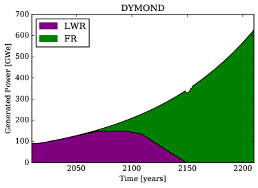
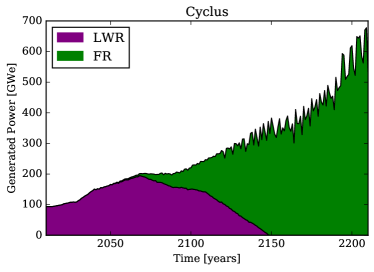
The demonstration here will use the generated power from LWRs and FRs in a transition that covers 200 years. The simulation should start with 90 GWe generated solely by LWRs and meet a 1% growth in demand over the lifetime of the simulation. Figure 1 shows the component time series curves for both DYMOND and Cyclus. From here, the benchmarking analysis may proceed.
3 Gaussian Process Modeling
The study of Gaussian processes is rich and deep and more completely covered by other resources, such as [4]. Here only the barest of introductions to this topic are given as motivated by the regression problem at hand. For nuclear fuel cycle benchmark analysis, Gaussian processes will be used to form a model of the metric time series over all simulators.
A Gaussian process is defined by mean and covariance functions. The mean function is taken to be the expectation value of the input functions, which here are the time series for all simulators. The covariance function is the expected value of the input functions to the mean. Symbolically,
| (2) |
| (3) |
The Gaussian process thus approximates the metric given information from all simulators. This is denoted either using functional or operator notation as follows:
| (4) |
Let indicate that the variable is associated with the model, rather than any of the raw simulator data.
For Gaussian process regression, a functional form for the covariance needs to be provided. This is sometimes called the kernel function and contains the free parameters for the regression, also called hyperparameters. How the hyperparameters are defined is tied to the definition of the kernel function itself. The values for the hyperparameters are determined via optimization of the maximal likelihood of the value of the metric function. While there are many possible kernels, a standard and generically applicable one is the exponential squared kernel, as seen in Equation 5:
| (5) |
Here, the length scale and the signal variance are the hyperparameters.
Now, define a matrix such that the element at the -th row and -th column is given by Equation 5. If a vector of training metric values is defined by concatenating metrics for all simulators for all times , then log likelihood of the obtaining is seen to be:
| (6) |
Here, is the modeling uncertainty as denoted in the previous section, is the identity matrix, and is the number of training points (the sum of the lengths of all of the time series). The hyperparameters and may be varied such that Equation 6 is minimized. In this way, an optimal model for the metric is obtained.
Finally, suppose we want to evaluate the Gaussian process regression at a series of time points . The covariance vector between this time grid and the training data is denoted as . The value of Gaussian process model of the metric function on the time grid is thus seen to be:
| (7) |
A full derivation of Equations 2-7 can be found in [4]. This resource also contains detailed discussions of how to optimize the hyperparameters, efficiently invert the covariance matrix, and compute the model values.
In practice, though, a number of free and open source implementations of Gaussian process regression are readily available. In the Scientific Python ecosystem, both scikit-learn v0.17 [13] and George v0.2.1 [6] implement Gaussian process regression. For the remainder of this paper, George is used for its superior performance characteristics and easier-to-use interface.
For purposes of nuclear fuel cycle benchmarking, Gaussian processes can be used to create models of each component feature (e.g. LWRs and FRs) from the results of all simulators together. Other regression techniques could also be used to create similar models. However, Gaussian processes have the advantage of incorporating modeling uncertainty, as seen above. The optimization of the hyperparameters yields the most accurate results for the model. Furthermore, the choice of kernel function can be tailored the functional form of the metric, if necessary. The exponential squared function was chosen because it is generic. If the metric is periodic, for instance, a cosine kernel may yield a more precise model. So while other regression techniques could be used, Gaussian processes encapsulate the correct behavior necessary for a non-judgmental benchmark while also remaining flexible to the particularities of the metric under examination.
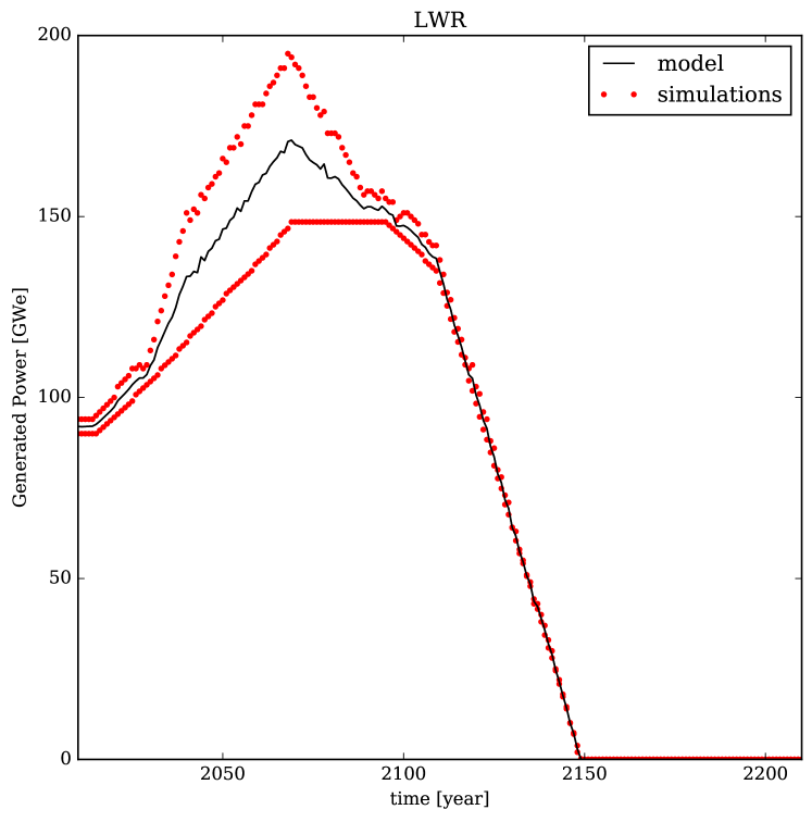
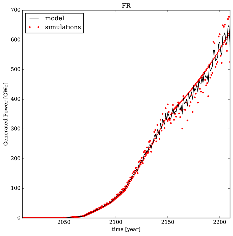
Using the sample data from §2, three models can be constructed: generated power from LWRs , generated power from FRs , and total generated power . Assuming only floating point precision as the metric uncertainty, these Gaussian process models can be seen in Figures 2 - 4 along with the original time series from the simulators that train the model. It is important to note that even though the sample data is only for two simulators, this method can handle any number of simulators, each with their own time grid, without modification.
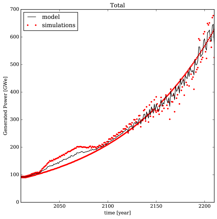
Also note that Figure 4 displays the model of the total generated power and not the total of the constituent models. Symbolically,
| (8) |
This is because the uncertainties are applied differently in these two cases. Moreover, the hyperparameter optimization would not be consistent if one were to sum up constituent models. It is thus considered safer to sum over the features for each simulator individually before applying the regression.
Thus far the metric data has had effectively zero uncertainty. But one of the desirable features of the Gaussian process regression is that it accounts for meaningful uncertainties. As a thought experiment, suppose that the time series data was much sparser and that the uncertainty associated with each value started off at zero and then grew at a rate of 1% per decade. A model of the total generated power with this uncertainty is shown in Figure 5.
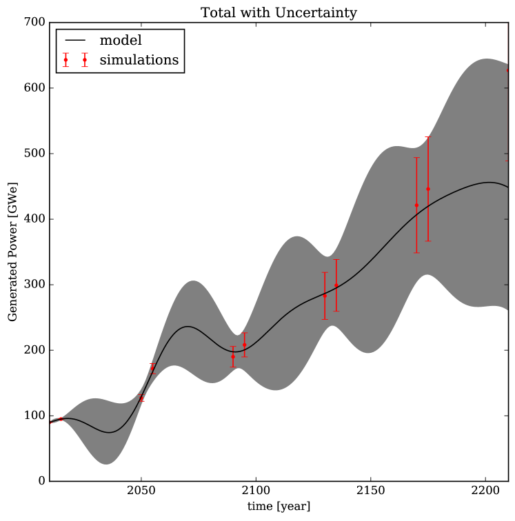
In Figure 5, note that as the model moves farther in time from the training data the standard deviation grows. Furthermore, as the uncertainty in the training data grows, the model itself degrades. Artifacts from the choice of kernel begin to be visible in model whenever the uncertainties are relatively high. Both of these match intuition about how uncertain systems should work.
Again, even though these uncertainty features are highly desirable in generic benchmarking applications, most nuclear fuel cycle simulators do not report uncertainties along with the metrics they compute. For this reason, the remainder of the examples in the paper will use the zero-uncertainty models as presented in Figures 2 - 4.
4 Dynamic Time Warping
Now that there are representative models of all time series, the issue at hand is how to compare these models. Dynamic time warping is a method for computing the distance between any two time series. The time series need not be of the same length. Furthermore, the time series may be decomposed into a set of representative spectra and the DTW may still be applied. The distance computed by DTW is a measure of the changes that would need to be made to one time series to turn it into (warp) the other time series. Thus, the DTW distance is a measure over the whole time series, and not just a single characteristic point. As with Gaussian processes, a number of more thorough resources, such as [5], cover dynamic time warping in greater detail. Here a minimal introduction is given that enables meaningful figure-of-merit calculations.
With respect to nuclear fuel cycle benchmarks, there are two main DTW applications. The first is to compute the distance between a Gaussian process model and each of the simulators that made up the training set for that model. This gives a quantitative measure of how far each simulator is from the model and can help determine which simulators are outliers. To maintain a non-judgmental benchmark, though, it is critical to not then use this information to discard outliers. Rather, outlier identification should be used as part of an inter-code comparison. If one simulator is an outlier for a given metric, the reasons for this should be investigated. For example, the outlier simulator may be at a higher fidelity level, there may be a bug in the outlier, or there may be a bug in all other simulators. Identifying outliers for many metrics could help discover the underlying cause of any discrepancies.
The second application of dynamic time warping to benchmarking is to compare the constituent feature models to the total model. Distances computed in this manner allow for a rank ordering of the components. This enables the benchmark to make claims about which features drive the fuel cycle metric most strongly, over the whole simulation time domain and for all simulators. Traditionally, the simulators have to agree within nominal error bounds () for a benchmark to make such a claim. Here, the simulators need not necessarily agree since the Gaussian process models are used as representatives. In this application, it is useful to recast the DTW distance as a measure of contribution. Contribution FOMs will be presented in §5.
For any two time series, dynamic time warping consists of three mathematical objects: the distance , a cost matrix , and a warp path . The cost matrix specifies how far a point on the first time series is from another point on the other time series. The warp path is then the minimal cost curve through this matrix from the fist point in time to the last. The distance, therefore, is the total cost of traversing the warp path.
The first step in a dynamic time warping algorithm is to compute the cost matrix. Suppose that the first time series has length indexed by and the second time series has length indexed by . It is helpful to define an matrix that is the norm of the difference of time series and :
| (9) |
The cost matrix is then an sized matrix that is defined by the following recursion relations:
| (10) |
The boundary conditions in Equation 10 are equivalent to applying an infinite cost to any or less than or equal to zero. The units of the cost matrix are the same as the units of the metric. However, the scale of the cost matrix is geometrically larger than the metric itself. This is due to the compounding nature of the recursive definition of .
Given , the warp path is thus a sequence of coordinate points that can then be computed by walking backwards through the matrix from to . For a point in the warp path, the previous point is given by where the cost is minimized among the locations one column over , one row over , and one previous diagonal element to . Symbolically,
| (11) |
The maximum possible length of is thus and the minimum length is . The warp path itself could potentially serve as a FOM. However, doing so would not take into account the cost along this path.
Therefore, the distance is defined as a FOM which does include for the cost of the warp. Due to the recursion relations used to define the cost matrix, can be stated succinctly as:
| (12) |
That is, is the final value of the cost matrix divided by the maximal length of the warp path.
For all practical purposes in nuclear fuel cycle benchmarking, and can be forced to have the same value. This is because the Gaussian process model can be used to predict a time series with whatever time grid is desired. The advantage of using a regression model is that it allows the analyst to force the same time grid. The advantage of dynamic time warping is that ensuring the same time grid is not necessary. Coupling Gaussian processes and DTW together is a more robust analysis tool than the methods individually.
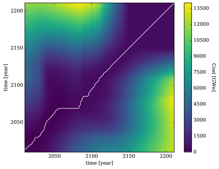
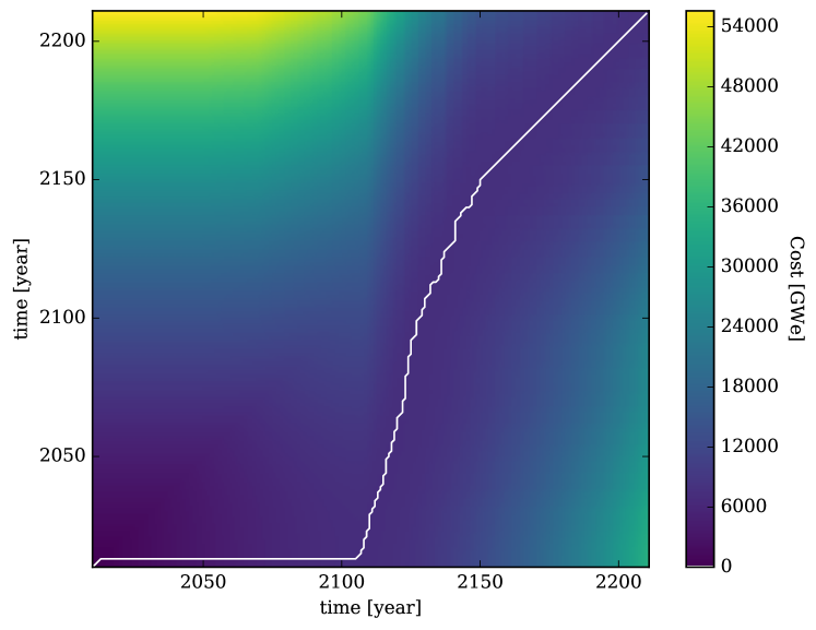
Figure 6 displays an example cost matrix as a heat map for the DTW between the LWR Gaussian process model and the original Cyclus LWR time series . Additionally, the warp path between these two is shown as the white curve on top of the heat map. Note that while is monotonic along both time axes, the path it takes minimizes the cost matrix at every step. Higher cost regions have the effect of pushing the warp path along one axis or another. The distance between these two curves is computed to be 1.053 GWe.
The process of dynamic time warping model generated data to raw simulator data can be repeated for all combinations of simulators and features. The that are computed may then directly serve as a FOM for outlier identification. Only distances between the same feature may be compared, as they share the same model. For instance, it is valid to compare and . However, it is not valid to compare and . In the situation, where the simulators have different time grids, the model can be evaluated with each time grid prior to computing the corresponding DTW distances and the comparison will remain valid.
| LWR | FR | Total | |
|---|---|---|---|
| DYMOND | 1.452 | 2.783 | 3.022 |
| Cyclus | 1.053 | 3.732 | 3.984 |
Table 1 gives the distances for all simulator and feature combinations in the sample data presented in §2. Only the differences between DYMOND and Cyclus for the same feature may be directly compared. However, Table 1 does indicate that the DYMOND is closer to the model since both the FR and Total generated power distances are closer for DYMOND than for Cyclus. As many simulators as desired could be added to the benchmark and distances could be tallied for them as well. At a sufficient number of simulators, usual statistics (mean, standard deviation) along each column may be computed. Simulators whose metrics fall outside of a typical threshold of the mean (one or two standard deviations) would then be considered outliers and subject to further inter-code comparison. The two simulators here are for demonstration purposes and neither can be said to be an outlier in a non-judgmental way. Recall, though, that outliers determined in this way may stem from the more correct simulator. The term outlier is not a condemnation on its own.
The second application of DTW to nuclear fuel cycle benchmarking is as a FOM for contribution of constituent features to a total metric. For this application, compute the distance between the model of the total and the model of the part, namely for all . This provides a measure of how much the total metric is determined by a particular part over the whole time series for all simulators. Using this measure is only reasonable if the total metric is known to be the sum of its constituents. This assumption is valid for a large percentage of nominal benchmarking metrics. In particular, mass flows and generated power both follow this rule. Metrics that are linear transformations of these basic metrics (such as decay heat or radiotoxicity) will also conform to this constraint. The distances computed here can then be used to rank order the importance of each constituent feature. Smaller distances are closer to the total and thus more important.
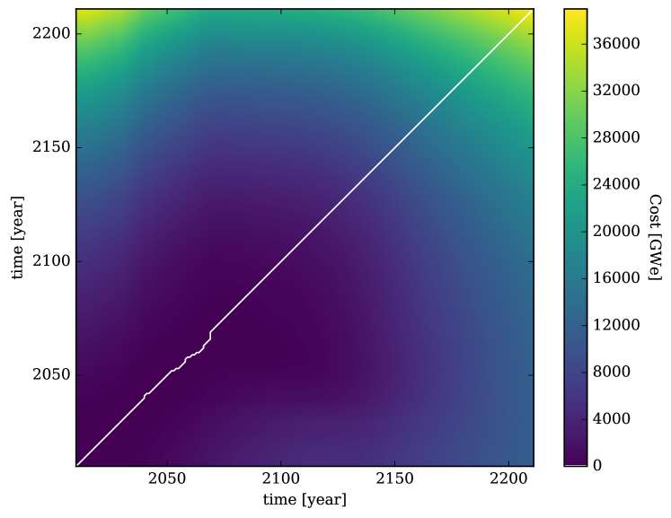
In the sample data here, the total generated power model can be compared to the models for LWR and FR generated power. The value of while . As expected, the FRs are a more important driver of the transition system than the LWRs over the time domain examined. Figures 7 & 8 show the cost matrices and warp paths for these two cases. Notice that in the FR case, the warp path is effectively flat until the FRs are deployed in significant numbers.
In summary, dynamic time warping yields a meaningful mechanism for benchmarks to compare various simulators and models. As a tool for outlier identification, it allows for each simulator to use its own native time grid. As a tool for performing rank ordering of features, the DTW distances are a perfectly functional FOM. However, lower distances implying higher importance may run counter to intuition. The potential for confusion, therefore, makes it less than ideal as a FOM on its own. A remedy for this is presented in the next section in form of a new contribution FOM.
5 Contribution
In §4, the dynamic time warping distance was presented as a FOM for measuring the similarity between time series, whether they were model-to-simulator comparisons or model-to-model comparisons. The distances alone, though, have the inverse meaning when trying to compute a FOM for contribution to a fuel cycle. For example, the question may be posed as, “Are LWRs or FRs more important to the fuel cycle as a whole?” While distances can answer this question, smaller disantances have higher impact. Preferably, a higher FOM score would yield a higher impact. Furthermore, the distances in the previous section have the same units as the cost matrix and are similarly bounded. A better FOM for contribution would be unitless and defined on the range .
Thus, let be the contribution FOM that satisfies the above constraints. To define , first define as the maximal possible distance from the model of the total. Recall that this time series has length . is, therefore, the L1 norm of the model of the total time series divided by twice its length.
| (13) |
This is the equivalent to computing the DTW distance between and the curve where the metric is zero for all time (i.e. the t-axis itself). This relies on the notion that metric is necessarily non-negative everywhere. If the metric is allowed to be negative, another baseline curve could be chosen. would then be computed as the DTW distance between the total model and this baseline. However, in most cases the metrics are not allowed to be negative, a baseline of zero is suitable, and Equation 13 applies.
The contribution figure-of-merit of a given partition to the total is thus defined as follows:
| (14) |
is seen to normalize the model-to-model distance while subtracting this ratio from unity makes higher contribution values more important. Using the sample data, and . This again shows that the FRs are more important to the total power of the whole cycle. Here though, higher contribution scores yield higher importance and the values are always between zero and one.
Note that even though is a fraction, it is not normalized across partitions. Namely, the sum of all contributions for all partitions is on the following range, which is not :
| (15) |
It is easy to imagine an alternative FOM that divides by . However, this was not done here because the choice of (the number of partitions) can be made arbitrarily large. In the sample calculations for LWRs and FRs. However, could have been set to 3 by including small modular reactor (SMRs) which are never built and produce no power. could then be increased to 4 or higher by including more non-existent reactor types. Dividing by is not stable enough for a FOM.
Furthermore, dividing the contribution by is not sufficient to normalize the sum of the , in general. This is because the contribution is inherently a cumulative measure. If a component ever had a non-zero value, it will always be seen to have contributed something. Because of this constraint on the total, can never reach unless there is only a single component or the total is zero valued everywhere (which implies that the constituents are also zero). Thus, dividing by with the aim of normalizing the sum of the is incorrect for any situation of interest to a fuel cycle benchmark.
If a truly normalized version of contribution is desired, it must use the sum of the actual contributions. Define the normalized contribution as ,
| (16) |
The disadvantage with the normalized contribution is that all of the individual component must be known prior to the normalization. Furthermore, since the sum is typically greater than 1, the difference between components is often smaller in the normalized form than in the more pronounced unnormalized contribution. The only advantages that confers over are that it is defined on the range and that . Otherwise, both versions of the FOM have the same properties.
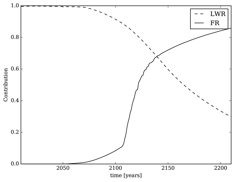
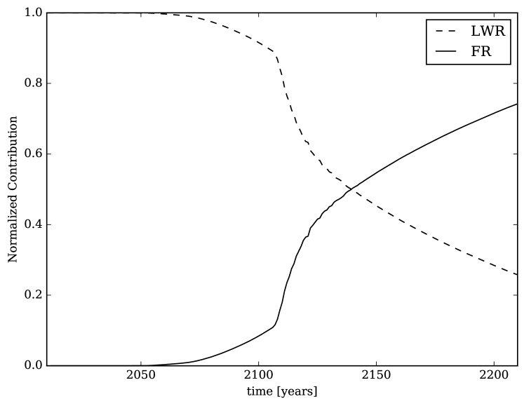
Both and can be viewed as a function of time. Doing so in a nuclear fuel cycle benchmark may help identify artifacts in the calculation that are the result of the time domain chosen for the benchmark itself. Figures 9 & 10 display the contribution and normalized contribution respectively for both LWRs and FRs over the full time domain. From these figures, the point where FRs become more important than LWRs is seen to be approximately year 2140.
6 Cautionary Tale on Filtering
It is tempting to insert standard filtering techniques from signal processing after creating a Gaussian process model but prior to any dynamic time warping calculations. A fast Fourier transform (FFT) based low-pass filter [14, 15] or Mel-frequency cepstral coefficients (MFCC) [8, 16] could be used to reduce error in the model itself, and thus make the contribution FOM more precise. Unfortunately, most fuel cycle metrics are not well-formed candidates for such filtering strategies. Including such filters as part of the analysis can easily lead to wildly unphysical models.
Consider a simple low-pass filter where a 256 channel real-valued FFT frequency transform is taken. All but lowest 32 channels are discarded prior to the applying the inverse transform. High frequency jitter in the original signal is removed, allowing for a better signal-to-noise ratio.
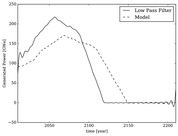
Figure 11 shows the results of applying the low-pass filter described above to the Gaussian process model of the LWR generated power, . The filtered curve demonstrates at least three major problems. The first is that the values of the curve are allowed to be negative, which is impossible for this (and many other) fuel cycle metrics. The second is that near the time boundaries ( and ), the amplitude of the filtered model is significantly higher than the unfiltered model. At , the metric should be zero but instead is 36.5 GWe. Thirdly, the shape of the curve itself is skewed to lower times. The time at which the metric goes to zero should be near year 2150 but is instead closer to year 2115. All of these issues would severely distort any DTW calculations that follow.
The reason behind these inconsistencies is that the FFT process is fundamentally periodic. However, using the annual time grid here, the LWR generated power metric is not periodic. Neither is the modeling error for most fuel cycle metrics periodic on an annual basis. Thus, while well-intentioned, a low-pass filter is not generally applicable.
Alternatively, MFCCs provide a mechanism for converting a time series into a set of power spectrum coefficient curves. Since the dynamic time warping procedure uses an L1 norm to form the cost matrix, the MFCCs of two signals can be directly compared. Each coefficient should roughly correspond in shape and amplitude to some feature in the original signal. Noisy, high frequency coefficients tend to be very similar and so their contribution to a DTW distance is correspondingly less than the contribution for lower mode coefficients. Coupling MFCC to DTW is an extremely common method employed in speech recognition systems [8, 17, 18].
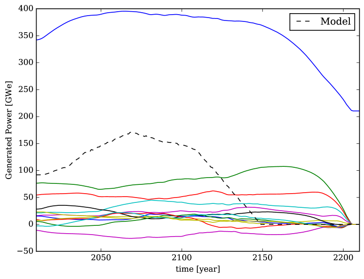
Figure 12 displays the MFCC curves of the LWR Gaussian process model as well as the model itself. None of these curves, not even the major coefficient, resembles the actual model. Rather, the cosine basis for MFCCs is clearly visible. As with the low-pass filter, the MFCCs also have uncharacteristic negative components. Moreover, the metric data is not sampled frequently enough to have meaningful time windows. For the fuel cycle metrics here, there is only one data point per year and the signal itself may change in a meaningful way each year. By comparison, in speech recognition, audio is sampled at least at 22050 Hz for characteristic signals on the order of 1 second. The data volume for fuel cycle benchmark metrics is simply too low for MFCC transformations to capture the desired features.
Proceeding anyways, suppose the contribution measure is computed for the MFCCs of LWR, FR, and total generated power models. In this case the LWR contribution is found to be 0.572 while the FR contribution is 0.899. Using the models directly as was done in §5, the contribution values were 0.298 and 0.859 respectively. This implies that using the MFCCs had the opposite effect as desired. The MFCCs added error to the FOM and made the LWR and FR contributions seem more alike than they truly are.
Therefore filtering the models prior to dynamic time warping is a dubious practice in the general case. In all likelihood, the metric does not meet the underlying assumptions of the filter. The metric may not be periodic or may not be sampled frequently enough. Sometimes it may be possible to construct a metric that does meet these qualifications. For instance, the generated power could be sampled monthly such that seasonal demand behavior is noticeable. Even in such a case, it is instead recommended to pick a different kernel for the Gaussian process model such that these periodic behaviors are captured. The regression itself then takes on the role of minimizing model uncertainty. Further filtering to this end becomes redundant and dangerous. Additionally, it is unlikely that the majority of the simulators would be able to calculate such a high-fidelity metric. That alone should disqualify such metrics or FOMs from any benchmarking study or inter-code comparison.
7 Conclusions & Future Work
This paper demonstrates a robust method for generating figures-of-merit for nuclear fuel cycle benchmarking activities by coupling Gaussian process regression to dynamic time warping. This method takes advantage of modeling uncertainties in fuel cycle metrics if they are known. It is also capable of handling the situation where different simulators output metric data on vastly different time grids. The distance computed by the dynamic time warping can itself serve as the figure-of-merit. Additionally, the distance can also be used to derive contribution and normalized contribution figures-of-merit.
Any regression method could have been used to form a model. Similarly, any mechanism for comparing two time series could have been used as a measure of distance. However, Gaussian processes and DTW were chosen because of the nature of a benchmarks and inter-code comparisons that lack experimental validation. It is not possible to build out a given fuel cycle scenario and see how it performs 200 years in the future. Furthermore, using historical data for validation provides too few cases for comparison and each simulator could simply be tuned to precisely match historical events. Thus, each simulator in a benchmark could be valid or they all could be invalid. It is therefore necessary for the FOM to not skew for or against any particular simulator. Gaussian process models as used here do not judge the simulators differently. The DTW then takes into account the cumulative effect of the whole time domain and does not preferentially select certain times.
The sample benchmark presented here was very simple and was used for motivation purposes only. It consisted of just two simulators (DYMOND and Cyclus) and one metric (generated power) with two components (LWR and FR). However, both Gaussian processes and DTW are inherently multivariate. More complex forms of analysis could therefore be performed. For example, the Gaussian process could jointly model the effect from many inputs onto the metric. Perhaps the benchmark is formulated to look at the generated power as a function of time and the power demand curve. In this case, a two dimensional GP model would be used. Alternatively, suppose that a matrix time series of the all individual nuclide mass flows are available. DTW is still able compute the distance between two such matrices. This would yield a measure of how the mass flows themselves differ - taking into account each nuclide component - without rely on a collapsed one dimensional total mass flow curve. Such cases will be considered in future work as real inter-code comparison data becomes available.
Furthermore, this work focused on the particular use case of benchmarking. However, the FOM calculations presented here could also be used to evaluate different fuel cycle scenarios. DTW distances could be computed between a business-as-usual once through scenario and an LWR-to-FR transition scenario, or any other proposed scenario. This provides a measure for comparing the relative cost (in units of the metric, not necessarily economic) for selecting one cycle over another. The work here, thus, should be seen as a stepping stone to further fuel cycle scenario evaluation work.
Lastly, dynamic time warping could itself serve a purpose as the objective function in a fuel cycle optimization. For example, suppose a power demand curve such as 1% power growth is known. The DTW distance from the total generated power to this curve could be minimized as a function of the reactor deployment schedule. Such a distance could potentially yield a more precise or faster optimization process than simply taking the sum of the differences between two time series. Such an optimization would also allow for matching on multiple time series features simultaneously while retaining a real-valued objective function.
Acknowledgements
The author would like to express deep gratitude to Dr. Bo Feng of Argonne National Lab for providing the DYMOND data used throughout this paper.
References
- [1] P. P. WILSON, “Comparing nuclear fuel cycle options,” Observation and Challenges (2011).
- [2] L. GUÉRIN et al., “A benchmark study of computer codes for system analysis of the nuclear fuel cycle,” , Massachusetts Institute of Technology. Center for Advanced Nuclear Energy Systems. Nuclear Fuel Cycle Program (2009).
- [3] S. J. PIET and N. R. SOELBERG, “Assessment of Tools and Data for System-Level Dynamic Analyse,” , INL/EXT-11 (2011).
- [4] C. E. RASMUSSEN and C. K. WILLIAMS, Gaussian processes for machine learning, The MIT Press (2006).
- [5] M. MÜLLER, “Dynamic Time Warping,” in Information Retrieval for Music and Motion, pages 69–84, Springer Berlin Heidelberg, 2007.
- [6] S. Ambikasaran, D. Foreman-Mackey, L. Greengard, D. W. Hogg, and M. O’Neil, “Fast Direct Methods for Gaussian Processes and the Analysis of NASA Kepler Mission Data,” (2014).
- [7] C. MYERS, L. R. RABINER, and A. E. ROSENBERG, “Performance tradeoffs in dynamic time warping algorithms for isolated word recognition,” Acoustics, Speech and Signal Processing, IEEE Transactions on, 28, 623 (1980).
- [8] L. MUDA, M. BEGAM, and I. ELAMVAZUTHI, “Voice recognition algorithms using mel frequency cepstral coefficient (MFCC) and dynamic time warping (DTW) techniques,” arXiv preprint arXiv:1003.4083 (2010).
- [9] A. YACOUT, J. JACOBSON, G. MATTHERN, S. PIET, and A. MOISSEYTSEV, “Modeling the Nuclear Fuel Cycle,” Proc. The 23rd International Conference of the System Dynamics Society," Boston, 2005.
- [10] B. FENG, “DYMOND EG01 to EG23 data,” private communication.
- [11] K. D. HUFF et al., “Fundamental Concepts in the Cyclus Fuel Cycle Simulator Framework,” CoRR, abs/1509.03604 (2015).
- [12] R. W. CARLSEN et al., “Cyclus v1.0.0,” (2014), http://dx.doi.org/10.6084/m9.figshare.1041745.
- [13] F. PEDREGOSA et al., “Scikit-learn: Machine Learning in Python,” Journal of Machine Learning Research, 12, 2825 (2011).
- [14] R. MERLETTI and P. DI TORINO, “Standards for reporting EMG data,” J Electromyogr Kinesiol, 9, 3 (1999).
- [15] K. MORELAND and E. ANGEL, “The FFT on a GPU,” Proc. Proceedings of the ACM SIGGRAPH/EUROGRAPHICS conference on Graphics hardware, pages 112–119, Eurographics Association, 2003.
- [16] S. IMAI, “Cepstral analysis synthesis on the mel frequency scale,” Proc. Acoustics, Speech, and Signal Processing, IEEE International Conference on ICASSP’83., volume 8, pages 93–96, IEEE, 1983.
- [17] B. MILNER and X. SHAO, “Speech reconstruction from mel-frequency cepstral coefficients using a source-filter model.,” Proc. INTERSPEECH, Citeseer, 2002.
- [18] N. SATO and Y. OBUCHI, “Emotion recognition using mel-frequency cepstral coefficients,” Information and Media Technologies, 2, 835 (2007).