A publicly available simulation of an enhanced network region of the Sun

Abstract

Context. The solar chromosphere is the interface between the solar surface and the solar corona. Modelling of this region is difficult because it represents the transition from optically thick to thin radiation escape, from gas-pressure domination to magnetic-pressure domination, from a neutral to an ionised state, from MHD to plasma physics, and from near-equilibrium (LTE) to non-equilibrium conditions.

Aims. Our aim is to provide the community with realistic simulations of the magnetic solar outer atmosphere. This will enable detailed comparison of existing and upcoming observations with synthetic observables from the simulations, thereby elucidating the complex interactions of magnetic fields and plasma that are crucial for our understanding of the dynamic outer atmosphere.

Methods. We used the radiation magnetohydrodynamics code Bifrost to perform simulations of a computational volume with a magnetic field topology similar to an enhanced network area on the Sun.

Results. The full simulation cubes are made available online. The general properties of the simulation are discussed, and limitations are discussed.

1 Introduction

The structure and dynamics of the outer solar atmosphere are set by magnetism. In the convection zone, the gas pressure exceeds the magnetic pressure in all but the strongest magnetic flux concentrations and the field is moved around by the plasma. These motions drive flows of energy and mass through the chromosphere into the corona. Most of the energy that is transported to the outer solar atmosphere through work done on the magnetic fields is radiated away in the chromosphere. It is also in the chromosphere that the dynamics change from gas-pressure-dominated behaviour to magnetic force dominance. The layer where the sound speed is equal to the Alfvén speed is located in the chromosphere, and conversion between different wave modes may occur. The ionization state goes from almost neutral to full ionization in the corona. The radiation goes from optically thick to optically thin, from local thermodynamic equilibrium (LTE) to non-equilibrium conditions. All these transitions make chromospheric physics very complicated, and the chromosphere may be the least understood region of the Sun (Judge & Peter 1998).

An early class of models of the solar chromosphere were 1D, semi-empirical models. Only in 1D was it possible to solve the non-LTE radiative transfer equations needed to produce synthetic observables that could be compared with observations. Since the energy transportation and dissipation mechanisms responsible for heating the chromosphere were unknown, the energy equation was replaced by treating the temperature as a function of height as a free parameter. Early reference models of this kind were the Bilderberg continuum atmosphere (BCA, Gingerich & de Jager 1968) and the Harvard-Smithsonian reference atmosphere (HSRA, Gingerich et al. 1971). With increased amounts of observables through continuum observations in the UV from Skylab, a series of models for six different components of the quiet solar chromosphere were constructed in a seminal series of papers (Vernazza et al. 1973, 1976, 1981), and the model corresponding most closely to the average quiet solar chromosphere, often denoted VAL3C, is the most cited solar chromospheric model. Later models have improved the fit in the temperature-minimum region (Avrett 1985; Maltby et al. 1986) and removed the need for a temperature plateau to reproduce the hydrogen Lyman-$\alpha$ line (Fontenla et al. 1990, 1991, 1993). See Rutten (2002) for an overview of 1D solar model atmospheres.

These models have been (and still are) very useful in providing model atmospheres with reasonable chromospheric conditions, and they can be used as numerical laboratories for exploring chromospheric line formation. It is important to keep in mind, though, that many different atmospheric models are consistent with a certain set of observables; Carlsson & Stein (1995) showed that a dynamic atmosphere with strong shocks gave the same temporal average UV continuum intensities as a VAL type model even though the average temperature structure was close to the radiative equilibrium solution.

Instead of using a trial-and-error way of adjusting the temperature structure, it is in principle possible to formulate an inversion strategy whereby the “best” model is arrived at through a formal definition of a “norm” and an automatic algorithm to minimise this norm. This can even be done in 3D including effects of an observational point spread function and the effects of 3D scattering (e.g., van Noort 2012; Socas-Navarro et al. 2015; Asensio Ramos & de la Cruz Rodríguez 2015). However, a fully unconstrained approach is ill-conditioned because there are more free parameters than observables. It is therefore crucial to develop proper strategies to arrive at physically motivated constraints in inversions.

The purpose of this paper is to describe a “realistic” numerical simulation of the solar outer atmosphere, extending from the upper convection zone to the corona, that is not determined by any fitting procedure to observations. By “realistic” we mean that we have gone to great lengths in trying to include the relevant physical processes in the numerical code and minimise the number of free parameters. Observations have thus NOT gone into constraining the model and a comparison of synthetic observables with observations will give information on what physics is missing in the numerical simulation. We also believe that the simulation sequence is very useful as a numerical laboratory to determine how observables depend on the atmospheric parameters. This will be true even if the models fail to reproduce certain detailed observations (which we already know is the case) as long as the model includes much of the important physics. For this reason it is important to have an understanding of what physics went into the model, what the approximations are, the general properties of the model and how they can be/cannot be used. This paper aims at providing such a detailed description.

A number of papers have used the simulation sequence described here. The formation of the H-$\alpha$ line was studied in Leenaarts et al. (2012), the Hanlé effect of Ly-$\alpha$ was studied by Štěpán et al. (2012, 2015) and the signatures of heating of the magnetic chromosphere were treated by de la Cruz Rodríguez et al. (2013). Loukitcheva et al. (2015) studied the diagnosing of the chromospheric thermal structure using millimeter radiation and Leenaarts et al. (2015) studied the nature of H-$\alpha$ fibrils in the solar chromosphere.

With the advent of chromospheric observations with high spatial and temporal resolution from the NASA Small Explorer satellite Interface Region Imaging Spectrograph (IRIS, De Pontieu et al. 2014b), we feel that it is crucial to use detailed numerical simulations, like the one presented here, in order to improve our understanding of what the observations tell us. This was also the initial driver for making this simulation sequence publicly available. A series of papers have been devoted to the formation of lines that are observable with IRIS: Leenaarts et al. (2013a, b); Pereira et al. (2013) treated the formation of the Mg ii h & k lines, Pereira et al. (2015) treated the formation of the Mg ii UV subordinate lines, Rathore & Carlsson (2015); Rathore et al. (2015) treated the formation of the C ii multiplet near 133.5 nm and Lin & Carlsson (2015) showed that the O i line at 135.56 nm is an excellent diagnostic of non-thermal velocities in the solar chromosphere. All these papers used snapshots from the current simulation as a laboratory for exploring line formation characteristics and relations between atmospheric conditions and observables.

The structure of this paper is as follows: In Section 2 we give a short description of the Bifrost code, in Section 3 we describe the general properties of the simulation sequence and in Section 4 we describe the data format and how to access the simulation data and we end with Discussion and Conclusions in Section 5.

2 Bifrost

The simulation described here has been performed with the 3D Radiation Magneto-Hydrodynamic (RMHD) code Bifrost. Bifrost is a general, flexible and massively parallel code described in detail in Gudiksen et al. (2011). In short, Bifrost solves the MHD equations on a staggered grid using a 5th/6th order compact finite difference scheme. The effects of radiation in the energy balance are taken into account by solving the radiative transfer equations along rays through the computational domain using a short-characteristic method and multi-group opacities (Nordlund 1982) with four opacity groups modified to take into account scattering (Skartlien 2000). See Hayek et al. (2010) for a detailed description of the treatment of the radiative transfer. Chromospheric radiative losses are calculated in non-LTE using simplified recipes (Carlsson & Leenaarts 2012) based on detailed 1D full non-LTE radiative transfer simulations using the RADYN code (Carlsson & Stein 1992, 1995, 1997, 2002). Optically thin radiative losses are taken into account using tables calculated from atomic data in CHIANTI, version 5 (Dere et al. 1997; Landi et al. 2006). Thermal conduction becomes important at high temperatures and is included using operator splitting with an implicit formulation based on a multi-grid method. Bifrost is an explicit code with diffusive terms in the equations in order to ensure stability. The diffusive operator employed is split in a small global diffusive term and a location specific hyper diffusion term, see Gudiksen et al. (2011) for details. In this simulation we do not include any terms taking care of ambipolar diffusion or Hall currents. Bifrost is a very general modeling code and a variety of modules are available for boundary conditions and the equation of state. For the simulation described in this paper we have included non-equilibrium ionization of hydrogen following the description by Leenaarts et al. (2007) based on the approximations by Sollum (1999). The background opacities are given by the old Uppsala background opacity package (Gustafsson 1973) and abundances are from Gustafsson et al. (1975).

3 Simulation

We have set up our simulation with the aim of studying processes in the solar chromosphere with a magnetic field configuration that we characterize as “enhanced network”. The computational box is 24 by 24 Mm² horizontally with periodic boundary conditions and extends 2.4 Mm below the visible surface (defined as the average height where optical depth at 500 nm is unity; this is also the zero point of our height scale.) and 14.4 Mm above encompassing the upper part of the convection zone, the photosphere, chromosphere, transition region and corona. The computational box is 504x504x496 grid points giving 48 km resolution horizontally and a variable grid separation in the vertical direction varying from 19 km in the photosphere and chromosphere up to 5 Mm height and then increasing to 100 km at the top boundary. Both the top and bottom boundaries are transparent. The top boundary is implemented using the characteristic equations (Gudiksen et al. 2011). At the bottom boundary, the magnetic field is passively advected with no extra field fed into the computational domain.

The simulation was initialised from a hydrodynamic simulation of size 6x6x3 Mm³ that had reached a relaxed state. This simulation reached 2.4 Mm below the visible surface but only 0.5 Mm above. The simulation was expanded horizontally (since it is periodic horizontally this just entails replicating the numerical domain to the larger size), first to 12x12 Mm² and then to 24x24 Mm². At each step small random perturbations were introduced and the simulation was run long enough that the horizontal periodicity from the startup vanished. The photospheric simulation was run for ten hours of solar time at a size of 24x24x3 Mm³. This relaxed hydrodynamic state was then expanded to 24x24x17 Mm³ by adding a chromosphere and corona in hydrostatic equilibrium and a temperature structure taken from a previous simulation. This temperature structure was just an initial condition and the temperature was not fixed in the following evolution. The time of the addition of the chromosphere and corona is taken as $t=0$ in the simulation. This state was allowed to relax for 1750 s of solar time to get rid of inconsistencies in the lower chromosphere. Because there is still no magnetic field, the upper part slowly cools and at $t=1750$ s the temperature at the upper boundary is 250 kK. At that point in time a large scale magnetic field was added.

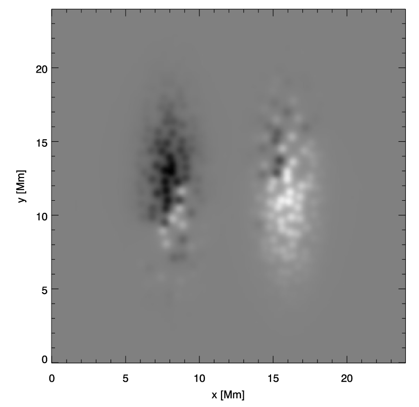
The magnetic field was added by specifying the vertical field at the bottom of the computational domain with a potential field extrapolation into the rest of the domain. The field at the bottom boundary was specified to have two patches of opposite dominant polarity separated by 8 Mm, with an overall balanced flux, see Figure 1. The magnetic field is very quickly swept to the downdrafts of the convective pattern and the potential character is also quickly lost in the upper part of the simulation. The moving around of the magnetic field by convection gives a Poynting flux into the upper part of the simulation. This magnetic energy is dissipated and creates a chromosphere and corona. The simulation was run assuming instantaneous hydrogen ionization equilibrium until the non-equilibrium hydrogen ionization was switched on at $t=3020$ s. The simulation was stopped at $t=5440$ s. The first published snapshot is snapshot 385 at $t=3850$ s. The various steps are given in Table 1

Table 1: Simulation timeline

time	event
(s)
-36000	24x24x3 Mm3 simulation extending to z=0.5 Mm
0	region added extending to z=14.4 Mm
1750	magnetic field added
3020	non-equilibrium hydrogen ionization switched on
3850	first published snapshot
5440	last published snapshot

Figure 1: Initial vertical magnetic field at the bottom of the computational domain. The maximum magnetic field strength is 0.8 kG (both in the bottom plane and the colour bar range) and the average signed field strength is close to zero (0.025 G).

3.1 Magnetic field

The computational box is too small to allow for the build-up of a magnetic field from global dynamo action. The field inserted at the bottom boundary, as described above, is the main free parameter of the simulation. It is therefore important to characterize the magnetic field that results from the continuous processing of the initial magnetic field by the convection.

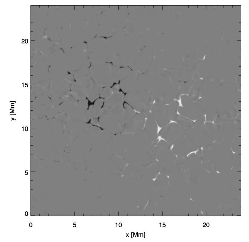
The average unsigned magnetic field strength in the photosphere is 48 G (5 mT). The vertical magnetic field at $z=0$ at $t=3850$ s (the snapshot used for most publications in the list in Section 1) is shown in Figure 2. The field has been swept to the intergranular lanes but the initial two dominant polarity patches separated by 8 Mm are still seen.

Figure 2: Vertical magnetic field strength at $z=0$ and $t=3850$ s. The field has been swept to the intergranular lanes. The maximum field-strength is 1.9 kG. The colour bar range is [-2 kG, 2 kG].

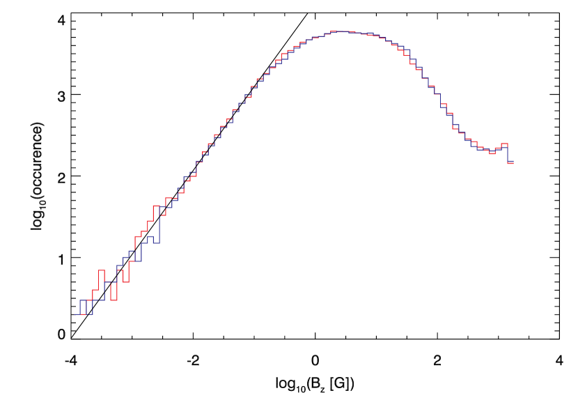
We can further characterize the magnetic field by the distribution of field-strengths. Figure 3 shows a histogram of the vertical magnetic field strength at $z=0$ at $t=3850$ s. There is no difference between the distributions of positive and negative $B_{z}$. The weaker field follows a power law distribution with a slope of one in the log-log diagram. The magnetic field distribution does not change significantly during the simulation timespan of 2420 s.

Figure 3: Histogram of the vertical magnetic field strength, $B_{z}$ at $z=0$ and $t=3850$ s for positive $B_{z}$ (red) and negative $B_{z}$ (blue). The straight black line shows a fit to the field with a strength below 0.1 G. The slope is 1.03 in the log-log plot.

The flux-based probability distribution (Steiner 2003) is shown in Figure 4. This probability distribution shows the fraction of the total absolute flux that has a flux density of less than a given value. From the figure we can see that 78% of the absolute flux at $z=0$ is in areas with a flux density less than 1 kG.

Figure 4: Flux-based probability distribution at $z=0$ and $t=3850$ s showing the fraction of the total absolute flux that has a flux density of less than $|$B$|$.

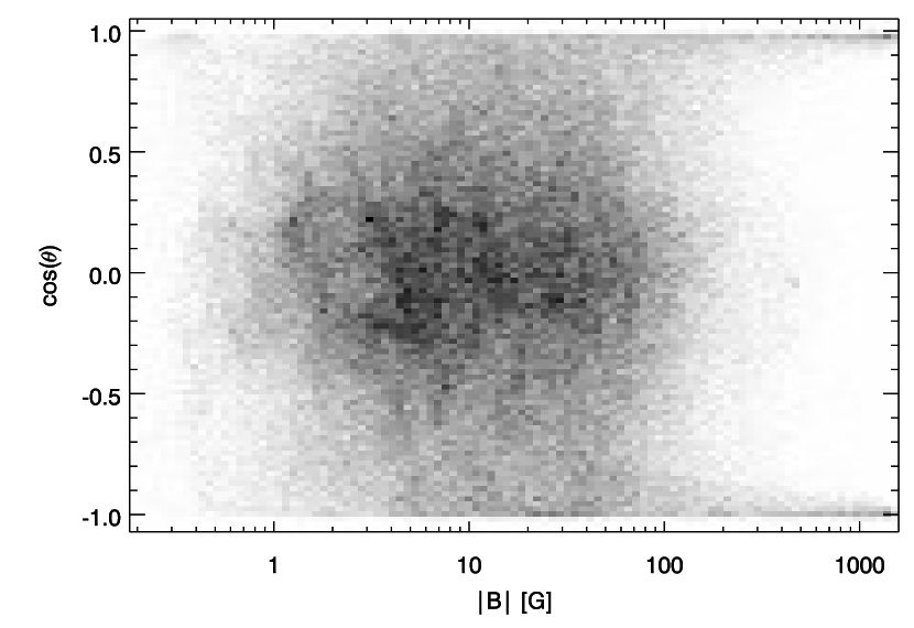
The distribution of field angles at $z=0$ is shown in Figure 5. Most of the field is pretty horizontal $|\cos(\theta)|<0.3$ but the strongest field ($|B|>300$ G) is vertical.

Figure 5: Joint probability distribution function (JPDF) of the cosine of the magnetic field angle to the vertical and the magnetic field strength at $z=0$ and $t=3850$ s.

The Joule heating in the simulation at heights from the upper photosphere to the corona scales roughly with the magnetic energy density, $B^{2}/(2\mu_{0})$ (Hansteen et al. 2010; Gudiksen & Nordlund 2005). Figure 6 shows the horizontally averaged magnetic energy density as a function of height in the snapshot at $t=3850$ s (it is very similar in other snapshots). The scaleheight of the magnetic energy density is about 0.4 Mm in the lower chromosphere ($z=0.2-1.2$ Mm) and increases to about 2 Mm scaleheight in the upper chromosphere and corona.

Figure 6: Horizontally averaged magnetic energy density ($B^{2}/(2\mu_{0})$) as function of height for the snapshot at $t=3850$ s. The scaleheight in the lower chromosphere ($z=0.2-1.2$ Mm) is 0.4 Mm and in the upper chromosphere and corona it is roughly 2.0 Mm (dotted lines).

3.2 Photosphere

The focus of the current simulation is the chromosphere and corona; for photospheric studies there are other simulations available with better numerical resolution, better description of the photospheric radiative transfer (e.g., more opacity bins) and more modern continuum opacity data (e.g., with the codes CO⁵BOLD, MURaM and Stagger, see Beeck et al. 2012, for a comparison of the codes). Our choice of background opacities from the old Uppsala package (Gustafsson 1973) was motivated by the availability of a well relaxed hydrodynamical model but is not the ideal choice if the aim is a detailed comparison of photospheric observables. It is also important to keep in mind that the effective temperature of the simulation is not set directly but only indirectly from specifying the incoming entropy at the lower boundary. The effective temperature thus varies in time with possible drifts with rather long timescales (set by the typical timescales at the bottom boundary). Figure 7 shows the temporal variation of the effective temperature of the simulation. Oscillations with periods of 350–500 s are seen (for a closer analysis, see Section 3.3) as well as a downward secular trend. The often used snapshot at $t=3850$ s has an effective temperature of 5773 K, close to the solar value.

Figure 7: Effective temperature as a function of time. The solar effective temperature of 5780 K is marked with a dotted line and the much used snapshot at $t=3850$ s (also the first published snapshot) with a star.

3.3 Oscillations

As is obvious in Figure 7, there are oscillations in the simulation box. The lower boundary is a pressure node reflecting acoustic waves to mimic the refraction of acoustic waves in the solar deeper atmosphere. The excitation of p-modes is similar to the real Sun but the energy is spread over a very limited set of modes giving them much larger amplitude (especially the global mode) compared with the Sun (Stein & Nordlund 2001). The horizontally averaged vertical velocity at eight heights, ranging from $z=-1.5$ Mm to $z=2.0$ Mm, is given in Figure 8. The average velocity in the photosphere (lower panel) is dominated by global oscillations that are in phase with a period of 450 s. At $z=0$, the average velocity is negative (upward) because the lower density in the granular upflows than in the intergranular downflows give a negative average velocity for a zero average massflux. At $z=0$ the amplitude of the oscillations is about 1 $\mathrm{km}\,\mathrm{s}^{-1}$. In the chromosphere (upper panel) we have a mixture of the global oscillations and propagating waves.

Figure 8: Horizontally averaged vertical velocity (positive is downflow) as function of time for eight heights (four in the upper panel and four in the lower panel, heights as given in the legend). The start of the published sequence of snapshots is indicated at $t=3850$ s as a grey line.

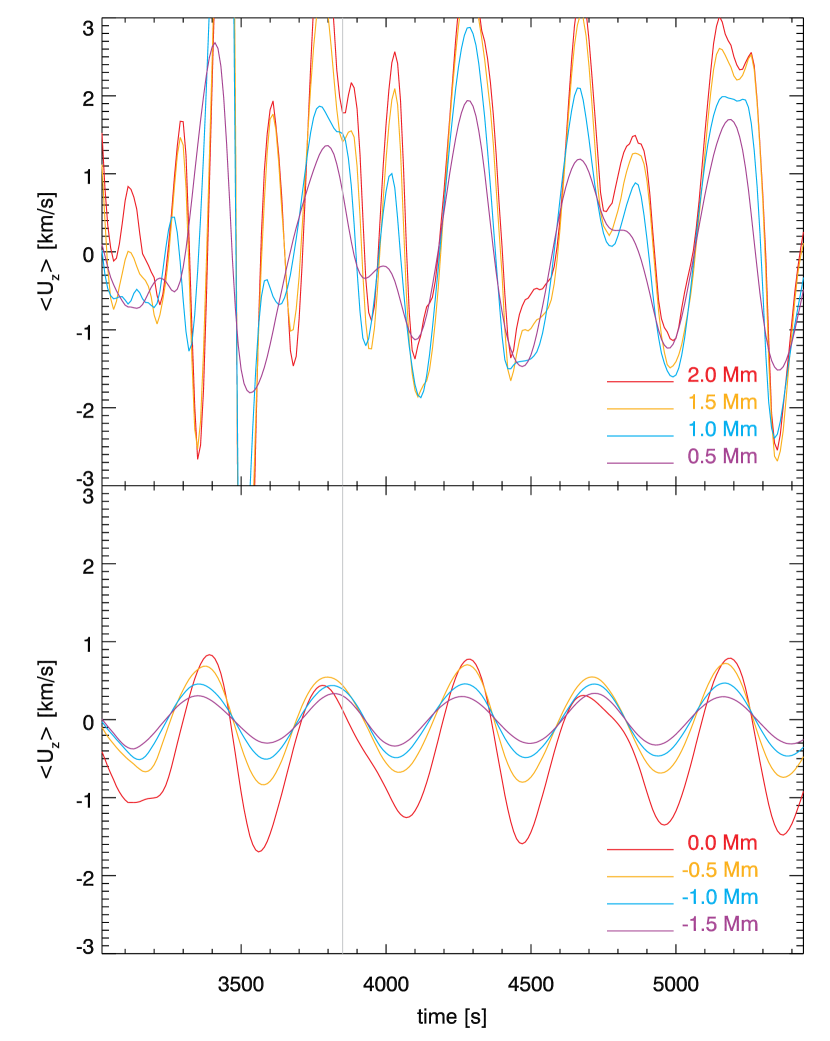
The height scale in the simulation is only approximately normalised to have a zero-point at optical depth unity at 500 nm (the usual zero-point of height-scales). Since there are oscillations in the simulation, the average height of $\tau_{500}=1$ varies in time with an amplitude of 60 km and a mean of 89 km, see Figure 9.

Figure 9: Average height of $\tau_{500}=1$ as function of time. The start of the published sequence of snapshots is indicated at $t=3850$ s as a grey line.

3.4 Temperature structure

The Joule heating caused by the braiding of the magnetic field from convective motions results in an increased temperature in the chromosphere and corona in the simulation. Additional heating comes from viscous dissipation. In this section we illustrate the temperature distributions found in the simulation but the detailed analysis of the energy balance is outside the scope of this paper.

The probability density function (PDF) of temperature as function of height at $t=3850$ s is shown in the upper panel of Figure 10. The spread in temperature at a given height is very small in the deep photosphere and increases in the subsurface layers, where we have hot granular upflows and cool intergranular downdrafts. There is a pronounced drop in temperature around $z=0$ and at $z=0.2$ Mm the temperature is restricted to a range between 4500 and 5500 K. Further up, there are both higher and lower temperatures with an average steady increase in the chromosphere up to a height of 2 Mm. Between 2 and 4 Mm height we encounter both chromospheric temperatures around $10^{4}$ K and transition-region to coronal temperatures up to $10^{6}$ K. From 4–14 Mm height we have temperatures up to slightly above $10^{6}$ K. There is a lower limit of 2400 K set by an artificial heating term that sets in as soon as the temperature drops below 2500 K. This is necessary in order to prevent the temperature from dropping to very low values in areas of rapid expansion (e.g., caused by the emergence of magnetic loops), see Leenaarts et al. (2011) for a discussion. There are relatively few points in the simulation box that are affected by this artificial limit in temperature. The bands of increased probability at temperatures of 10 kK and 20 kK are caused by the ionization of helium that is treated in LTE in the current simulation, see Golding et al. (2014) for a discussion of non-equilibrium effects of helium ionization. At the end of the simulation run, at $t=5440$ s, the distribution is rather similar to the situation at $t=3850$ s in the chromosphere, but the corona has been further heated such that the regions with temperatures below 300 kK above a height of 5 Mm are now gone, with the exception of an extended helium ionization region at 10 kK.

Figure 10: Probability density function (PDF) of the temperature as function of height at $t=3850$ s (upper panel) and at $t=5440$ s (lower panel). Note the logarithmic temperature scale.

Figure 11: Volume rendering of the temperature distribution at $t=5440$ s viewed from the top (left) and side (right). $B_{z}$ at $z=0$ with positive (red) and negative (blue) polarity. The Moiré patterns are artefacts of the volume visualisation.

Figure 12: Same as Figure 11 for $\log_{10}T=5.2-6.1$

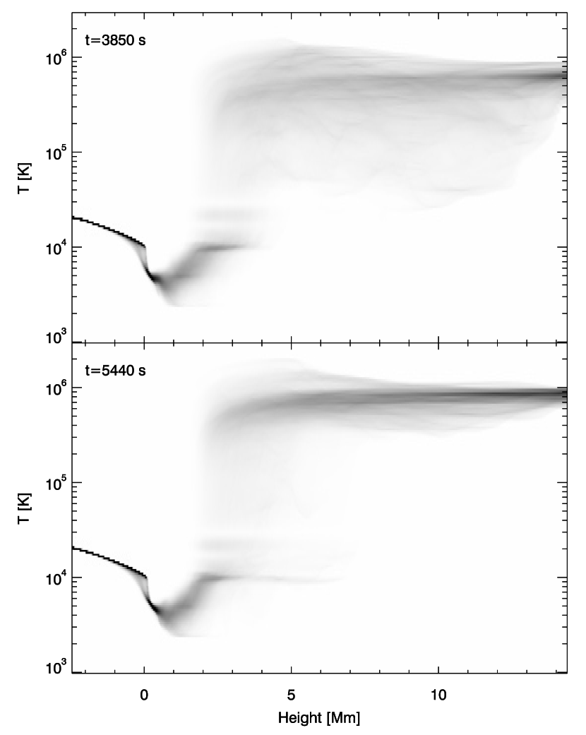
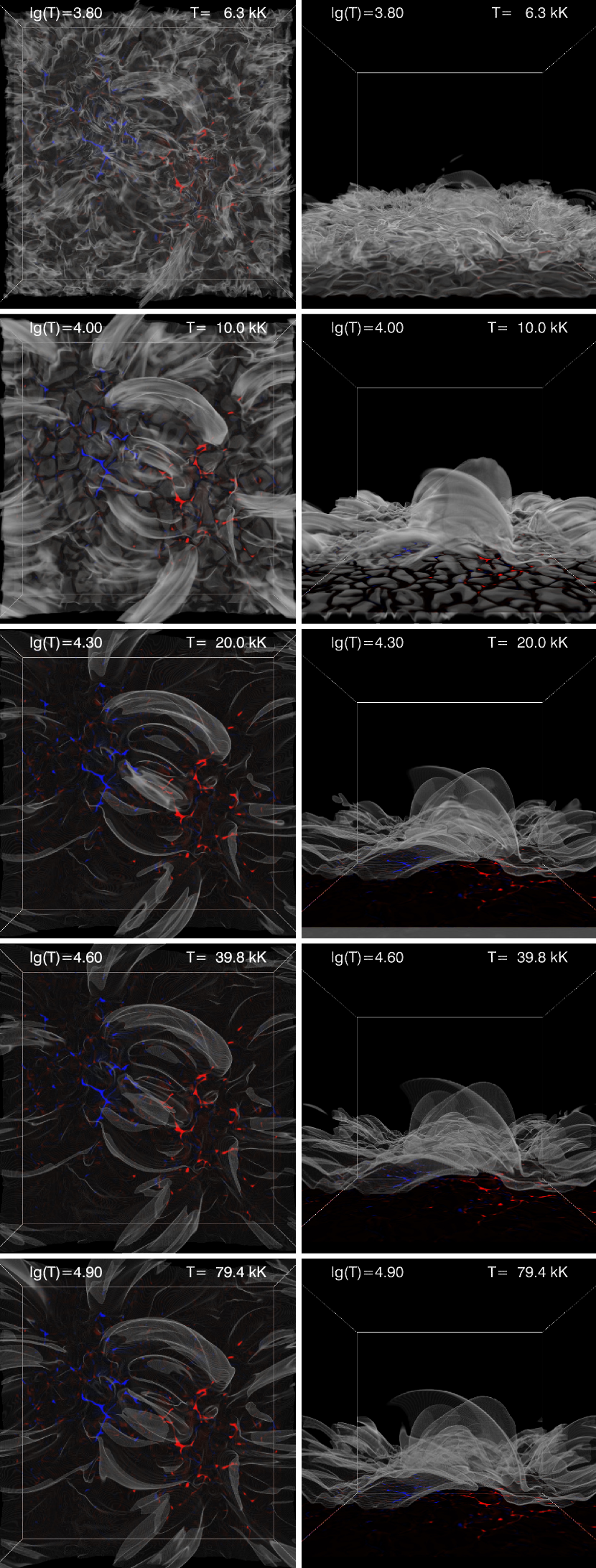
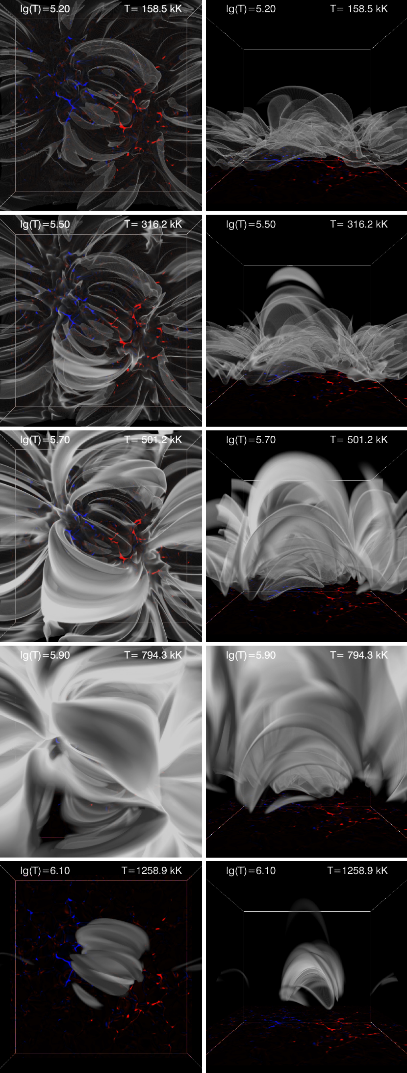
As is obvious from Figure 10, the temperature is not a single valued function of height; there is a large spread of temperatures at most heights. Figures 11–12 show the spatial distribution of the plasma at different temperatures. Each panel shows the distribution of plasma at a given temperature with a triangular shaped weighting centred on a given logarithmic temperature with a range of $\pm 0.05$ in the logarithm. Note that there is no weighting with density (as would be appropriate for an optically thin spectral line with a given formation temperature).

At a temperature of 6.3 kK we already see low lying loop structures connecting magnetic field of opposite polarities. There is a multitude of these low lying, short loops but much of the plasma at that temperature is also distributed in structures that are less loop-like. At 10 kK most of the lowest lying loops have disappeared and we have fewer, more pronounced loops that reach higher. At higher temperatures we basically see the same loops, all the way up to 316 kK ($\log_{10}(T)=5.5$) when a new set of hotter, higher lying loops start to appear. These loops dominate up to about 1 MK. The maximum temperature in this simulation is 2.2 MK and this hottest plasma is located in loops that do not reach as high as the loops with temperatures up to 1 MK.

The lower lying loops with temperatures below 300 kK evolve on shorter timescales than the hotter loops and give rise to the ”Unresolved Fine Structure” (UFS) loops discussed in Hansteen et al. (2014).

3.5 Ionization balance

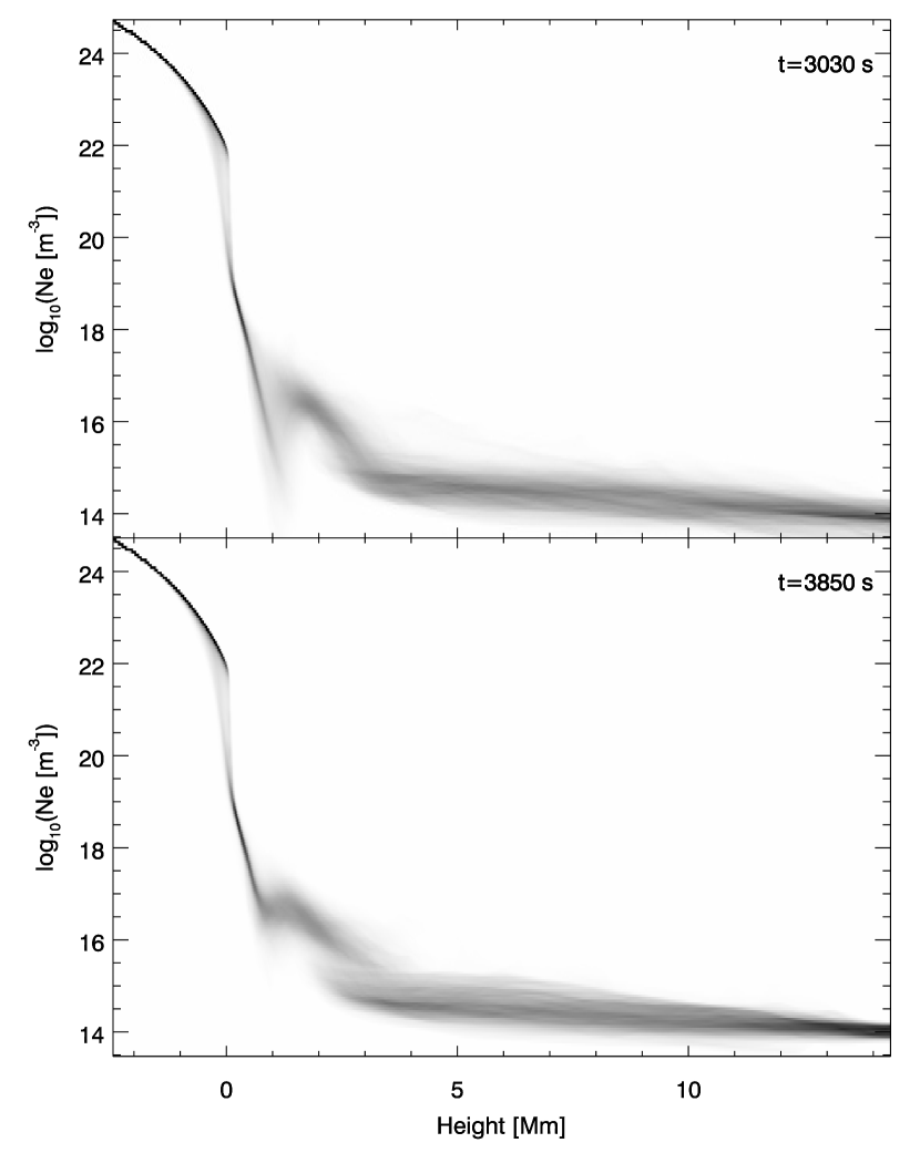
The simulation includes the effects of non-equilibrium ionization of hydrogen, see Leenaarts et al. (2007). Figure 13 shows the electron density as a function of height for two times, just 10 s after the non-equilibrium ionization of hydrogen was switched on at $t=3030$ s and for the first published snapshot, at $t=3850$ s. The non-equilibrium hydrogen ionization leads to much higher electron density in the cool pockets at 0.5–2 Mm and also higher electron densities up to 3.5 Mm height. There is not much change with time of this probability density function after $t=3850$ s.

Figure 13: Probability density function (PDF) of the electron density as function of height at $t=3030$ s (upper panel) and at $t=3850$ s (lower panel). Note the logarithmic electron density scale.

3.6 Velocity field

Spectral lines are normally observed to be broader than what the thermal broadening of the opacity profile would give. An extra free parameter, called microturbulence, is often introduced in 1D semi-empirical models to account for this broadening. The ”micro” in the name comes from the fact that this parameter is introduced as an extra broadening of the opacity profile, acting in exactly the same way as thermal broadening. This would be a physically correct description in the limit of zero length-scale for the velocity field. It is also often necessary to introduce a second free parameter to account for the observed lineshape. This is called macroturbulence and is equivalent to a Gaussian convolution of the emergent intensity profile (rather than a convolution of the opacity profile as is the case for microturbulence). Realistic 3D radiation hydrodynamic simulations of the solar photosphere give line profiles that are close to the observed profiles without the addition of extra free parameters — the non-thermal broadening comes from Doppler shifts arising from the convective flows and oscillations (e.g., Asplund et al. 2000).

Also spectral lines formed in the outer atmosphere are broader than what thermal broadening alone predicts. The nature of this non-thermal broadening in the outer atmosphere is still unclear, but the presence of strong shocks (Carlsson & Stein 1992, 1997; De Pontieu et al. 2015), torsional motions (De Pontieu et al. 2014a), and Alfvén wave turbulence (van Ballegooijen et al. 2011) are some of the candidates.

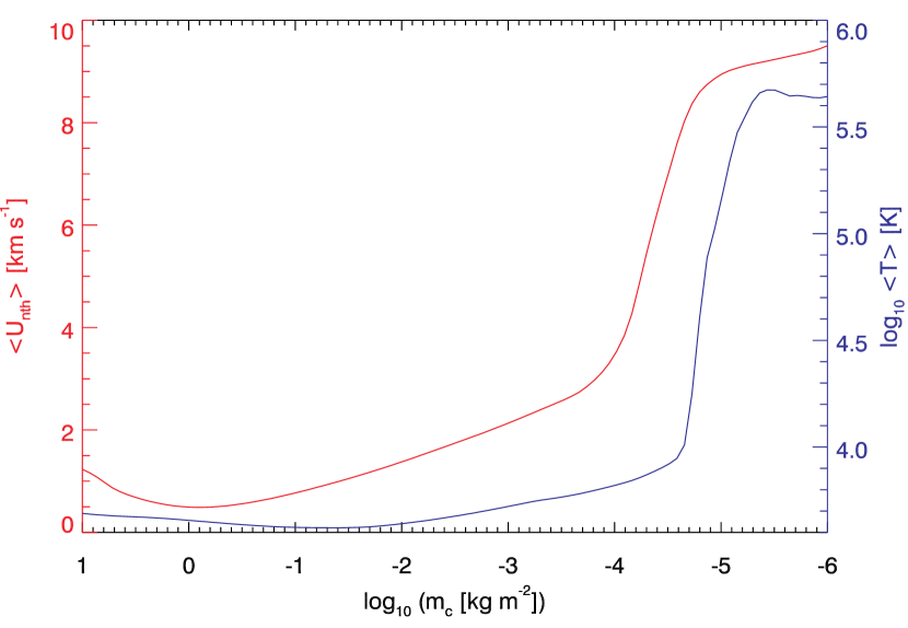
There is no simple way to characterize the macroscopic velocities in the simulation that give rise to non-thermal broadening. The effect of a given velocity field on the spectral line width depends on whether the spectral line is optically thick or optically thin, where in the atmosphere the line is formed and the width of the contribution function to intensity. One possible way of quantifying the velocity field is the standard deviation of the vertical velocity over a given height range as function of height and horizontal position. At each column of the simulation box at $t=3850$ s we calculate the column mass scale (which is more closely related to line formation quantities like optical depth than a geometric height) and take the standard deviation of the vertical velocity over a range of $\pm 1$ dex in $\log_{10}$(column mass). We multiply the standard deviation by the square root of two in order to get a quantity that can be directly compared with microturbulence and call this quantity non-thermal velocity, $U_{\rm nth}$. The average over planes of constant column mass is shown in Figure 14. The temperature averaged over planes of constant column mass is also shown. The transition region is situated around $\log_{10}(m_{c}\mathrm{[kg\,m}^{-2}\mathrm{]})=-5$ (equivalent to a logarithmic value of $-6$ in cgs units). The average non-thermal velocity rises steadily from 0.5 $\mathrm{km}\,\mathrm{s}^{-1}$ at zero logarithmic column mass to 3.5 $\mathrm{km}\,\mathrm{s}^{-1}$ at $\log_{10}(m_{c})=-4$. Through the transition region, the average non-thermal velocity in the simulation rises to 9 $\mathrm{km}\,\mathrm{s}^{-1}$. These values are quite a bit smaller than are needed to explain the non-thermal broadening of optically thin spectral lines formed in the chromosphere (4-8 $\mathrm{km}\,\mathrm{s}^{-1}$; Carlsson et al. 2015). and lower transition region ($\approx 20$ $\mathrm{km}\,\mathrm{s}^{-1}$; De Pontieu et al. 2015).

Preliminary results from simulations run at higher spatial resolution (horizontal grid size of 31 km instead of 48 km) indicate that part of the explanation may be the limited numerical resolution of the current simulation: in the 31 km simulation the non-thermal velocity at $\log_{10}(m_{c})=-3$ increased from 2.1 $\mathrm{km}\,\mathrm{s}^{-1}$ to 3.4 $\mathrm{km}\,\mathrm{s}^{-1}$, the rapid increase in non-thermal velocity happens already at $\log_{10}(m_{c})=-3.5$ and the value in the transition region increases to 15 $\mathrm{km}\,\mathrm{s}^{-1}$.

Figure 14: Average non-thermal velocity calculated over $\pm 1$ dex in $\log_{10}$(column mass) (red, left scale) and average temperature (blue, right scale) as function of logarithmic column mass for the simulation snapshot at $t=3850$ s.

4 Data access

The full simulation cubes with all variables as function of grid position are available from the Hinode Science Data Centre Europe (http://www.sdc.uio.no/search/simulations).

Each timestep saved to file is called a snapshot and they are numbered from $t=0$ with 10 s of solar time separating each snapshot. The first published snapshot is snapshot 385 at $t=3850$ s, which is 830 s after the switch on of the non-equilibrium hydrogen ionization when the initial startup effects have largely disappeared. The last snapshot is at $t=5440$ s giving a timespan of 1590 s for the published simulation.

All files are in FITS format with a format similar to IRIS level 2 data: 3D cubes of data ($x$,$y$,$z$) with one variable per file. The $x$- and $y$-grids are equidistant and can be generated using the standard FITS keywords while the $z$-grid is non-uniform and is therefore given in a FITS extension.

The file names are of the form BIFROST_en024048_hion_<var>_<snap>.fits where the runname en024048_hion comes from ”enhanced network”, 24 Mm horizontal size, 48 km horizontal grid-spacing and hion because the simulation includes non-equilibrium ionization of hydrogen. <var> is the variable name, listed in Table 2, and <snap> is the snapshot number.

Table 2: Available variables

variable	explanation
lgr	$\log_{10}$(mass density)
ux	bulk velocity in $x$
uy	bulk velocity in $y$
uz	bulk velocity in $z$
lge	$\log_{10}$(internal energy)
bx	magnetic field strength in $x$
by	magnetic field strength in $y$
bz	magnetic field strength in $z$
lgne	$\log_{10}$(electron density)
lgp	$\log_{10}$(gas pressure)
lgtg	$\log_{10}$(temperature)

All variables are cell centred on a right-handed system with $z$ increasing upwards. Index runs the same way as the axis which means that $z$[1] is at the bottom and $z$[nz] at the top. Note that this is different from the original Bifrost files.

All units are SI units and given in FITS keywords (Mm, m/s, kg m/s, T, W/m³, nm, etc). Specifically this means that magnetic field strength is given in Tesla (1 T=$10^{4}$ G).

Metadata is given in the FITS header. This data release is part of the IRIS project and an explanation of the FITS keywords is given in IRIS Technical Note 33 (the IRIS Technical Note series is available from http://iris.lmsal.com). Software to analyse the simulation data is provided in SolarSoft (http://www.lmsal.com/solarsoft) with descriptions in IRIS Technical Note 34. Synthetic observables are also made publicly available at the Hinode Science Data Centre Europe; so far only the spectrum around the Mg II h & k lines but more will follow, see IRIS Technical Note 35.

Papers published based on the simulation presented here should cite both the code description paper (Gudiksen et al. 2011) and this paper.

5 Discussion and Conclusions

We have presented the main characteristics of a Bifrost simulation aimed at the study of the outer solar atmosphere. The main free parameter is the initial magnetic field configuration. The field configuration of the current simulation, named en024048_hion, is characterised by two opposite polarity patches separated by some 8 Mm in a box of horizontal extent 24 Mm $\times$ 24 Mm.

It is important to take into account the characteristics when analysing the simulation or synthetic observables derived from it. The major caveats presented above are:

• The opacities and abundances are from old tables, basically from Gustafsson (1973); Gustafsson et al. (1975), in order to be compatible with earlier deep convection simulations. These opacities and abundances are not ideal for comparison of synthetic observables with detailed photospheric intensities.

• The effective temperature is not specified in the simulation and is only set by specifying the entropy of the incoming fluid at the bottom boundary. The relaxation to a given effective temperature is a very slow process and in the en024048_hion simulation the effective temperature is typically lower than that of the Sun, see Section 3.2.

• There are major oscillations in the simulations, see Section 3.3.

• The height scale is only approximately normalised to have a zero-point close to optical depth unity at 500 nm (the usual zero-point of height-scales). Since there are oscillations in the simulation, the average height of $\tau_{500}=1$ varies in time, see Section 3.3

• The published data have all variables specified at the same location (cell-centres) instead of being on a staggered grid as in the original simulation. This means that the variables that originally are not given at cell-centres (velocities and magnetic field strength) have been interpolated to cell-centres with the same high-order interpolation scheme as used in Bifrost. This introduces interpolation noise, in particular the divergence of B is no longer zero to the machine accuracy as is the case for the original data.

The paper series on ”The formation of IRIS Diagnostics” (see Section 1) contains several comparisons of synthetic observables from this simulation with observations. It is clear from these comparisons that the simulation lacks important physics, even for the quiet sun. In particular chromospheric spectral lines synthesised from the simulation tend to be too weak and too narrow. The comparisons indicate that the simulation has too small amplitude mass motions at small spatial scales (the ”non-thermal broadening” of spectral lines is too small) and too little plasma at chromospheric temperatures. However, the parameter space exhibited by the simulation seems to cover typical chromospheric conditions (albeit not in the right proportions) and we hope the simulation sequence published here can serve as a useful laboratory to further our understanding of the outer solar atmosphere.